Evaporation-driven convective flows in suspensions of non-motile bacteria

Abstract

We report a novel form of convection in suspensions of the bioluminiscent marine bacterium Photobacterium phosphoreum. Suspensions of these bacteria placed in a chamber open to the air create persistent luminiscent plumes most easily visible when observed in the dark. These flows are strikingly similar to the classical bioconvection pattern of aerotactic swimming bacteria, which create an unstable stratification by swimming upwards to an air-water interface, but they are a puzzle since the strain of P. phosphoreum used does not express flagella and therefore cannot swim. Systematic experimentation with suspensions of microspheres reveals that these flow patterns are driven not by the bacteria but by the accumulation of salt at the air-water interface due to evaporation of the culture medium; even at room temperature and humidity, and physiologically relevant salt concentrations, the rate of water evaporation is sufficient to drive convection patterns. A mathematical model is developed to understand the mechanism of plume formation, and linear stability analysis as well as numerical simulations were carried out to support the conclusions. While evaporation-driven convection has not been discussed extensively in the context of biological systems, these results suggest that the phenomenon may be relevant in other systems, particularly those using microorganisms of limited motility.

I Introduction

In the deep ocean animals such as certain fish and squid produce light through a symbiotic relationship with bioluminescent bacteria FarmerIII2006 . This luminscence requires oxygen and is regulated by the process of quorum sensing, which guarantees that photons are only emitted when the bacterial concentration is sufficiently high Dunlap2006 . One well-known luminiscent bacterium is Photobacterium phosphoreum, a rod-shaped organism $\sim\!3.5$ $\mu$m long and $\sim\!0.5$ $\mu$m wide, whose bright luminscence can easily be observed when a flask containing a sufficiently concentrated suspension is swirled gently to oxygenate the fluid. If instead the suspension is placed in a cuvette like that shown in Fig. 1 then after several minutes, during which the bacteria deplete the oxygen and bulk luminiscence fades away, a novel phenomenon of bright convective plumes is observed. In the figure, which was taken in the dark, regions of blue are luminiscent and have a high concentration of oxygen. Careful observation shows that the fluid within the plumes flows downward from the meniscus and the luminscence within gradually fades as the fluid descends and recirculates in convective rolls.

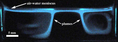
Figure 1: Convective flow observed in a suspension of Photobacterium phosphoreum. The chamber is $6$ cm long, $1$ mm deep and $1$ cm high. Bacteria were cultured to a density of  $5.5\times 10^{8}$ cells/cm³ following the procedure detailed in the text. This image was acquired with Nikon D300s equipped with a 60 mm f/2.8 macro lens, and an exposure time of 10 seconds.

The convection pattern in Fig. 1 appears to be a classic example of bioconvection Pedley1992 , an instability that arises from the accumulation of swimming microorganisms at the top surface of a suspension typically in response to chemical gradients or light. As most cells are denser that the suspending fluid, upwards chemo- or phototaxis creates an unstable nonuniformity in the cell concentration which triggers convective motion. Yet, the strain of P. phosphoreumused in our experiments is non-motile under the given conditions, presumably as a consequence of generations of culturing in rich media in which expression of flagella is not triggered. Given this, the macroscopic flow in Fig. 1 cannot be rationalized as a classical bioconvective instability.

An alternate explanation for the observed convective patterns observed is that a metabolic reaction, for example the chemical reaction that produces bioluminescence, may release a component that is denser than the background fluid. This idea was motivated by examples of so-called chemoconvection in the methylene-blue glucose system, where the chemical reaction creates a product that alters the local buoyancy balance Pons2000 . Using similar arguments, Benoit et al. Benoit2008 explained the buoyant plumes observed in a suspension of non-motile Escherichia coli consuming glucose.

As will be explained in detail below, a series of control experiments allows us to discard the hypothesis that a chemical reaction or metabolic activity creates the plumes. Instead, we find that the convection arises from evaporation of the salty suspension. A prior report of evaporation-induced convection was presented by Kang et al. Kang2013 , where flows in a sessile droplet of salty water were observed by adding fluorescent beads. They noticed that the flow was first oriented towards the perimeter of the drop, in the same way as it moves in the coffee stain phenomenon Brown1827 ; Deegan1997 . An accumulation of salt occurrs at the surface of the drop, which triggers convective motion. The proposed mathematical model introduces the “salinity Rayleigh number” $Ra_{s}$ by analogy with the Rayleigh number used to predict the onset convection in a fluid heated from below Rayleigh1916a . The salinity Rayleigh number compares the buoyancy generated by the accumulation of salt with the stabilizing effects of salt diffusion and fluid viscosity. This concept as been used previously in the literature to explain the double-diffusion in the phenomenon of salt fingering Singh2014 , and it has been also found to be essential to understand the accumulation of salt in saline groundwater lakes Wooding1997 .

This paper is organized as follows: Sec. II describes the experimental setup and quantitative observations of plumes. In the next two sections a mathematical model is introduced, which is based on the coupling of the Navier-Stokes equation for the evaporating fluid with an advection-diffusion equation for the salt. This model is first studied in Sec. III using linear stability analysis, and then numerically using a finite element method in Sec. IV. A comparison between experiments, linear stability analysis and numerical results is presented in section V. Finally, conclusions and future work are summarized in Sec. VI.

II Experimental metehods and results

II.1 Culturing of P. phosphoreum

Table 1 shows the ingredients for the liquid and solid media used in the experiments with P. phosphoreum. Bacterial cultures were streaked on agar plates and kept in an incubator at 19^∘C in the dark, and renewed every two weeks. Liquid cultures were prepared by picking a bright colony from an agar plate and adding it to $50$ ml of bacterial culture, which was then shaken at $100$ rpm in an incubator in the dark at 19^∘C. After $15$ hours of shaking, the bacterial suspension reached an optical density OD${}_{600nm}\sim 1$. For long term storage, the strain was frozen at $-80^{\circ}$C using the cryoprotective medium described by Dunlap and Kita-Tsukamoto Dunlap2006 , although using 65% (v/v) glycerol in equal parts worked equally well. The relation between OD and number of bacteria was found using the technique of serial dilution together with the track method. We found that OD_600nm=1 corresponds to  $5\times 10^{8}$ bact/ml.

Table 1: Liquid and solid medium used to grow P. phosphoreum.

Liquid medium (for 1L)		Solid medium (for 1L)
Peptone	10g	Nutrient broth powder	8 g
sodium chloride	30g	sodium chloride	30 g
glycerol	2 g	glycerol	10 g
di-potassium hydrogen phosphate	2 g	calcium carbonate	5 g
magnesium sulphate	0.25 g	agar	15 g

II.2 Setup

Suspensions were studied in chambers of the form shown in Fig. 2a, constructed from two glass coverslips (Fisher 12404070) held together by two layers of tape 300 $\mu$m thick (Bio-Rad SLF-3001). This tape has internal dimensions $6\times 2$ cm, and one long side was cut to create an air-liquid interface. The cuvette, 600 $\mu$m in depth, was filled using a plastic syringe connected to a stainless steel needle (Sigma-Aldrich CAD4108). The cuvette was filled with sufficient suspension to yield a fluid height of $1$ cm, which is the initial condition for the model presented in Secs. III and IV. Figure 2b is a schematic representation of the dark field setup used to observe the plumes. From left to right, the elements in this setup are a charge-coupled device (CCD) camera (Hamamatsu C7300) to capture dark field images, the sample, and a red light-emitting diode (LED) ring (CCS FPR-136-RD). The camera is placed in the dark spot inside of the cone formed by the rays coming from the LED ring. Placing a sample where the rays meet will result in light being deflected or scattered by the the suspended particles toward the camera.

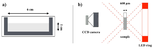
Figure 2: Experimental method. (a) Cuvette used in the experiment made with two coverslips held together by 600 $\mu$m thick tape cut in a U-shape. (b) Dark field imaging system where the dashed lines represent the light coming from the LED ring.

II.3 Bacteria versus beads

The hypothesis that the chemical reaction leading to light production in P. phosphoreum  created dense components that trigger hydrodynamic plumes was excluded by two control experiments. The first one consisted of placing non-motile, non-bioluminescent bacteria in the same experimental setup. A genetically modified strain of Serratia (ATCC 39006), provided by Dr. Rita Monson (Department of Genetics, University of Cambridge), also created the plumes observed with P. phosphoreum, even though this bacterium does not produce light when it consumes oxygen. The second and most important control experiment came from using 3 $\mu$m diameter polystyrene beads (Polyscience 18327) at a similar optical density (OD) as in the experiments with P. phosphoreum. Figure 3 shows side by side experiments with (a) bacteria and (b) bead suspended in the same bacterial medium and observed using the dark field technique (see Supplemental videos $1$ and $2$ suppl ). In these experiments we sealed the top boundary except for one small hole (indicated by an arrow) which allowed evaporation. We found that the position of the plume is precisely correlated with the position of the source of evaporation. Note in particular that the center of the plumes is depleted of bacteria or beads, an important feature discussed later.

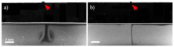
Figure 3: Control experiment. P. phosphoreum (left) and 3 $\mu$m beads (right) were placed in the cuvettes described in Fig. 2 but in this case the top boundary was closed except for a single hole (indicated by red arrows). Both experiments were performed at optical density OD${}_{600nm}=1.5$ and the images were taken $75$ minutes after the experiment started.

As the plume generation does not depend on any life processes of the bacteria, in subsequent experiments described below we focused exclusively on suspensions of microspheres instead of bacteria. Switching to beads also allowed us to explore a wide range of salt concentrations, far beyond that which is physiologically possible using P. phosphoreum.

II.4 Experiments using beads

Figure 4 shows convective patterns observed in a suspension of 3 $\mu$m diameter microspheres in a 1% (weight/weight) salt solution (see also Supplemental video $3$ suppl ). The bright horizontal line at the top of the image is the air-water meniscus. Note that the plumes appear dark in the dark field image, which means an absence of particles deflecting light in those regions. This situation is very different from conventional bioconvection, in which the plumes appear bright due to the relatively higher bacterial concentration within them.

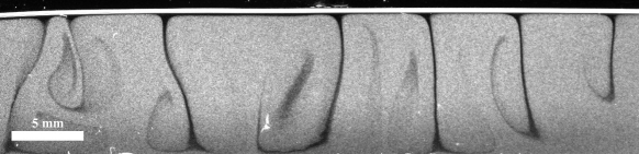
Figure 4: Convection in a microsphere suspension. Dark field image of the plumes observed in a suspension of 3 $\mu$m diameter beads with 1% (w/w) salt concentration. The optical density was $OD_{600nm}$=1 and the image was taken 30 minutes after the experiment had started.

A protocol was designed to find the positions of the plumes in time for different salt concentrations. An image like that in Fig. 4 was first cropped near the top surface, keeping the horizontal length but narrowing in the vertical direction. After converting to black and white with a threshold of $0.5$, the greyscale was inverted. Then, a one-dimensional plot was generated by averaging the pixel intensity vertically, where noise was reduced by applying the Matlab function smooth. The peaks were found using the function findpeaks with the condition that the peaks be greater than $0.4$ mm apart. Figure 5 shows the plume positions corresponding to the conditions of Fig. 4, where different colors represent the position of the first plume, second plume, and so on until the seventh plume. In this representation a given plume can change color because a new plume appeared at the left side.

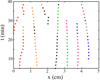
Figure 5: Plume dynamics. Graphical representation of the plume position in time for an experiment using 3 $\mu$m diameter beads and 1% (w/w) salt concentration. Different colours indicate the position of the first plume (red), second (orange), third (black), fourth (green), fifth (pink), sixth (blue) and seventh (grey).

Figure 6 shows convection in suspensions with (a) $0.1$% (w/w) salt and (b) $0.01$% (w/w) salt. Comparing these images to that in Fig. 5 one can see that for smaller salt concentrations the thickness of the plumes and the spacing between them both increase. When these experiments were analyzed using the code described above, the average distance between plumes using 1% salt concentration was $\lambda_{exp,1\%}=0.67\pm 0.06\mbox{ cm}$, while for 0.1% was $\lambda_{exp,0.1\%}=1.58\pm 0.08\mbox{ cm}$. In 0.01% suspensions it was difficult to determine the wavelength although it is clearly larger than when using ten times more salt.

Another feature in these experiments is that the less salt in the suspension, the longer it takes to observe the appearance of plumes. This can be seen in Fig. 6 where both images were taken once the instability developed: for 0.1% it occurred after 1 hour, while for 0.01% a full 10 hours was needed.

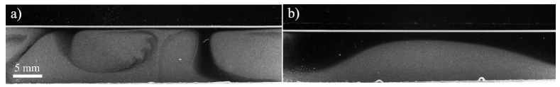
Figure 6: Plumes at different salt concentration using $2.17$ $\mu$m polyestyrene beads. (a) $0.1$% (w/w) salt concentration, $1$ hour after beginning of the experiment. (b) $0.01$% (w/w) salt concentration, $10$ hours after the experiment started. The initial height for both experiments was $1$ cm, and in the image on the right the effect of evaporation can be seen by the lower meniscus.

II.5 Plume mechanism

In the experiments presented above, the plumes appear black in the dark field imaging method, which means that there are no beads inside the plumes. Our hypothesis is that these dark plumes are a consequence of the sedimentation of beads; while salt is accumulating at the upper fluid surface due to evaporation the beads are continuously sedimenting, and once the instability starts, the convective flows carry fluid down from the top surface, which is depleted of beads. This idea was investigated by performing the experiments using beads of different sizes, thereby changing the sedimentation speed, while keeping the mean salt concentration fixed. Fig. 7 shows the plumes observed using monodispersed polystyrene beads $3$ $\mu$m in diameter (Polyscience 09850-5) and $6$ $\mu$m in diameter (Polyscience 07312-5). It is readily apparent that the plumes using larger beads are also wider. In this low Reynolds number regime the Stokes law for sedimentation holds, with a speed proportional to (radius)², so the larger beads sediment four times faster. Using ImageJ the thickness of the plumes in both cases were measured at three different points, obtaining $\mbox{d}_{3\mu m}=0.152\pm 0.008\mbox{ mm}$, while $\mbox{d}_{6\mu m}=0.590\pm 0.025\mbox{ mm}$, very consistent with the ratio of the sedimentation speeds.

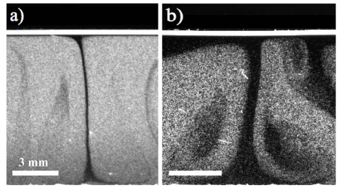
Figure 7: Effect of microsphere size. Plumes using $3$ $\mu$m diameter beads (a) and $6$ $\mu$m beads (b). The material, initial height, and salt concentration are the same in both cases. The optical density in both cases is OD_600nm=1 and the images were taken $45$ minutes after the experiment had started.

The role of salt in the plume formation was tested by suspending the beads in pure water. After $27$ hours of observation no plumes appeared, confirming that the presence of salt is necessary to create the convection (this experiment was repeated three times). From these experiments it was also verified that the thermal effect of evaporation is not strong enough to produce plumes under our experimental conditions. Finally, evaporation was avoided by adding a layer of mineral oil on top of the solution of water and 1% (w/w) salt, which is the same salt concentration used in the experiment in Fig. 4). After $10$ hours no plumes were observed, while the air-fluid interface remained fixed. This experiment highlighted the importance of evaporation in accumulating salt at the interface.

In summary, experimental results have shown: a) the center of the plumes is depleted of beads, b) the thickness of the plumes is directly related to the sedimentation rate of beads, c) plumes do not appear when beads are suspended in pure water, and d) evaporation is needed to observe plumes. Based on these observations, the following mechanism for plume formation is proposed. Initially, the system has a nearly homogeneous distribution of beads. Before the instability starts, beads sediment, and an accumulation of salt is built up at the air-water interface during this time. When the salt concentration at the top surface has reached a critical value, the hydrodynamic instability is triggered by a buoyancy imbalance, carrying down the fluid near the top surface which contains no beads.

III Linear stability analysis

The hypothesis that accumulation of salt due to evaporation is responsible for plume formation is studied in this section using linear stability analysis. A classical example of the use of this technique is in explaining Rayleigh-Bénard convection, observed when a fluid is heated from below, in which an instability arises as a consequence of the thermal expansion of the fluid. Bénard’s observations in 1900 Benard1900 were followed by Rayleigh’s analytical work in 1916 Rayleigh1916a , which established that the instability takes place when what we now term the Rayleigh number $Ra$ exceeds a critical value. $Ra=\beta_{T}\alpha gd^{4}/\kappa\nu$ compares the buoyancy force with the dissipative forces (viscosity and thermal diffusion), where $\beta_{T}$ is the temperature gradient, $\alpha$ the coefficient of thermal expansion, $g$ the acceleration due to gravity, $d$ the depth of the fluid layer, $\kappa$ the thermal diffusivity and $\nu$ the kinematic viscosity.

The calculation presented here uses a salinity Rayleigh number that compares the buoyancy created by salt with the stabilizing effects of salt diffusion and fluid viscosity. It is

$$Ra_{s}=\frac{\beta c_{0}gd^{3}}{D\nu},$$ (1)

where $\beta$ is the solute expansion coefficient (which gives the change in suspension density due to the salt concentration), $c_{0}$ is the initial salt concentration, and $D$ is the salt diffusion constant. It is important to note that the salinity Rayleigh number has often been defined in the literature using the change in salinity between top and bottom instead of the initial salt concentration (see for example Ref. Renardy1996 ). Yet, even an initially uniform concentration profile will create a gradient due to evaporation, so the present definition is more useful here, and was adopted by Kang et al. Kang2013 .

The problem analyzed in this section is a laterally infinite two-dimensional cuvette filled with a saline solution. The salt concentration is initially homogeneous with a value $c_{0}$ and the initial height of the column of water is $h_{0}$ ($1$ cm in the experiments). Evaporation has the effect of decreasing the fluid height $h(t^{*})$ at a constant speed $v_{e}$, so we assume

$$h(t^{*})=h_{0}-v_{e}t^{*}.$$ (2)

III.1 Governing equations

The dynamics of the salt concentration $c^{*}$ follow the advection-diffusion equation

$$\frac{\partial c^{*}}{\partial t^{*}}+\nabla\cdot(c^{*}{\bf u^{*}})=D{\nabla^{2}}c^{*},$$ (3)

with $D$ the salt diffusion constant, and ${\bf u}^{*}$ the velocity field. For the fluid flow, the Navier-Stokes equations with the Bousinesq approximation are used:

$$\nabla\cdot{\bf u^{*}} =0,$$ (4a)

$$\frac{\partial\bf{u^{*}}}{\partial t^{*}}+\bf{u^{*}}\cdot\nabla{\bf u^{*}} =-\frac{\nabla p^{*}}{\rho_{0}}+\nu\nabla^{2}{\bf u}^{*}-\frac{\rho}{\rho_{0}}g\hat{{\bf k}}.$$ (4b)

Eq. (4a) is the incompressibility condition, and in Eq. (4b) $p^{*}$ is the pressure, $\rho_{0}$ the fluid density in the initial state with a homogenous distribution of salt, $\nu$ is the kinematic viscosity, $\rho$ the density of the fluid considering the salt distribution, $g$ is the acceleration of gravity, and $\hat{{\bf k}}$ is the unit vector in the vertical direction.

To account for the moving top boundary we normalize the vertical direction by the instantaneous height $h(t^{*})$, while the horizontal direction is normalized by $h_{0}$, yielding dimensionless quantities

$$z=\frac{z^{*}}{h(t^{*})},\hskip 14.22636ptx=\frac{x^{*}}{h_{0}},\hskip 14.22636ptt=\frac{D}{h_{0}^{2}}t^{*}.$$ (5)

With these definitions and making use of a dimensionless height

$$H=\frac{h(t)}{h_{0}},$$ (6)

and the Péclet number

$$Pe=\frac{h_{0}v_{e}}{D},$$ (7)

the dynamics of the salt concentration in terms of dimensionless variables is

$$\frac{\partial c}{\partial t}=-Pe\frac{z}{H}\frac{\partial c}{\partial z}+\frac{\partial^{2}c}{\partial x^{2}}+\frac{1}{H^{2}}\frac{\partial^{2}c}{\partial z^{2}}-u\frac{\partial c}{\partial x}-\frac{w}{H}\frac{\partial c}{\partial z}.$$ (8)

In the equation for the fluid flow, the notation ${\bf u}=(u,w)$ is introduced to identify the horizontal and vertical components of the fluid velocity. The incompressibility condition is

$$\frac{\partial u}{\partial x}+\frac{1}{H}\frac{\partial w}{\partial z}=0,$$ (9)

and the Navier-Stokes equations for the fluid flow are

$$\frac{\partial u}{\partial t}=-Pe\frac{z}{H}\frac{\partial u}{\partial z}-u\frac{\partial u}{\partial x}-\frac{w}{H}\frac{\partial u}{\partial z}-\frac{\partial p}{\partial x}+S\!c\left(\frac{\partial^{2}u}{\partial x^{2}}+\frac{1}{H^{2}}\frac{\partial^{2}u}{\partial z^{2}}\right),$$ (10)

in the horizontal direction, and

$$\frac{\partial w}{\partial t}=-Pe\frac{z}{H}\frac{\partial w}{\partial z}-u\frac{\partial w}{\partial x}-\frac{w}{H}\frac{\partial w}{\partial z}-\frac{1}{H}\frac{\partial}{\partial z}\tilde{p}+S\!c\left(\frac{\partial^{2}w}{\partial x^{2}}+\frac{1}{H^{2}}\frac{\partial^{2}w}{\partial z^{2}}\right)-Ra_{s}S\!c\left(c-1\right),$$ (11)

in the vertical direction, where the pressure as $\tilde{p}=p-gzH$ and $S\!c=\nu/D$ is the Schmidt number. Finally, the rescaled height evolves as

$$H(t)=1-Pe\,t.$$ (12)

Typical values of the experimental and material parameters are given in Table 2.

Table 2: Numerical values of the parameters used in the calculations

Parameter	Symbol	Value
Kinematic viscosity of water	$\nu$	$10^{-6}$ m2/s
Salt diffusion constant	$D$	$10^{-9}$ m2/s
Salt expansion coefficient	$\beta=\rho_{0}^{-1}\partial{\rho}/\partial{c}$	0.007 (w/w)-1
Initial height	$h_{0}$	10-2 m
Evaporation rate	$v_{e}$	$2\times 10^{-8}$ m/s
Péclet number	$Pe=h_{0}v_{e}/D$	$0.2$
Schmidt number	$S\!c=\nu/D$	$10^{3}$

III.2 Base state

Equations (8), (10) and (11) are now linearized around a base state, which is assumed to be homogeneous in the $x$ direction:

$$\frac{\partial}{\partial x}=0,~{}~{}\frac{\partial}{\partial x}\Big{|}_{t=0}=0.$$ (13)

Then, the continuity condition enforces $\partial w/\partial z=0$. Given the boundary condition $w=0$ at $z=0$ and $\partial w/\partial z=0$ at $z=1$, the fluid must be at rest, i.e. $\mathbf{u}_{0}(t,z)=(0,0)$. Similarly, $c=c_{0}(z,t)$ satisfies Eq. (8) in the absence of fluid flow,

$$\frac{\partial c_{0}}{\partial t}=\frac{1}{H^{2}}\frac{\partial^{2}c_{0}}{\partial z^{2}}-\frac{P_{e}z}{H}\frac{\partial c_{0}}{\partial z}.$$ (14)

To find the boundary conditions for $c_{0}$ it is useful to go back to the dimensionful equations and then translate them to dimensionless variables. Integrating the conservation equation along the z-direction,

$$\int_{0}^{h(t)}\left(\frac{\partial c_{0}^{*}}{\partial t^{*}}-D\frac{d^{2}c_{0}^{*}}{dz^{*2}}\right)dz^{*}=0,$$ (15)

and using the Leibniz integral rule for the first term, we obtain

$$\int_{0}^{h(t)}\frac{\partial c_{0}^{*}(z^{*},t^{*})}{\partial t^{*}}dz^{*}=\frac{\partial}{\partial t^{*}}\left(\int_{0}^{h(t)}c_{0}^{*}(z^{*},t^{*})dz^{*}\right)-c_{0}^{*}(h(t^{*}),t^{*})\,\,\,\frac{dh(t^{*})}{dt^{*}}.$$ (16)

Because the total amount of salt in the system is constant, the first term on the right hand side of Eq. (16) vanishes. Then, by using Eq. (16) in (15), we obtain

$$D\frac{dc_{0}^{*}}{dz^{*}}\biggr{\rvert}_{z^{*}=h(t)}=-c_{0}^{*}(h(t^{*}),t^{*})\,\,\,\frac{dh(t^{*})}{dt^{*}}=c_{0}^{*}v_{e}\biggr{\rvert}_{z^{*}=h(t)},$$ (17)

where the constant evaporation rate $v_{e}$ was identified. Returning to the dimensionless variables, the upper boundary condition is

$$\frac{dc_{0}}{dt}\biggr{\rvert}_{z=1}=PeHc_{0}\biggr{\rvert}_{z=1}.$$ (18)

Similarly, at $z=0$ the boundary condition of zero flux implies $dc_{0}/dz=0$. Finally, the initial condition for the salt concentration is a homogenous distribution, therefore $c_{0}(z,0)=1$.

Equation (14) with the initial and boundary conditions described above was solved numerically using the function “pdepe” pdepe in Matlab, yielding an approximate solution on a given one dimensional grid. The dimensionless concentration $c_{0}$ as a function of the dimensionless vertical direction $z$ is plotted in Fig. 8, where different colours represent the salt profiles after a given numbers of hours. In the figure it is possible to observe how the salt accumulates near $z=1$, and how the overall concentration increases as a result of the decrease in height while the total amount of salt is conserved.

Figure 8: Base state. Normalized salt concentration as a function of the normalized $z$-direction. The plot corresponds to the numerical solution of Eq. (14) with no-flux boundary conditions (18) and no flux at $z=0$, with $Pe=0.2$, calculated from experimental parameters. The colors correspond to different elapsed times since start of evaporation.

III.3 Linearized equations for small perturbations

The timescale required to evaporate the suspension completely, around 50-100 hours, is much longer than the tens of minutes over which plumes develop, and therefore it can be assumed that the timescale $t$ of the plume dynamics is much shorter than that needed to reach a base state ($t_{0}$). The first step to linearize Eqs. (8), (10) and (11) is to consider a small perturbation around the base state at order $\varepsilon$ such that

$${\bf u}({\bf x},t) ={\bf 0}+\varepsilon{\bf u}^{\prime}({\bf x},t)+O(\varepsilon^{2}),$$ (19a)

$$c({\bf x},t) =c_{0}(z,t_{0})+\varepsilon c^{\prime}({\bf x},t)+O(\varepsilon^{2}),$$ (19b)

$$p({\bf x},t) =p_{0}(z,t_{0})+\varepsilon p^{\prime}({\bf x},t)+O(\varepsilon^{2}),$$ (19c)

where ${\bf u}^{\prime}=(u^{\prime},w^{\prime})$ is the perturbed velocity field, and $c^{\prime}$ is the perturbed salt concentration. Substituting Eqs. (19c) into Eqs. (8), (10) and (11), and collecting the terms at $O(\varepsilon)$, we obtain

$$\frac{\partial c^{\prime}}{\partial t} =-P_{e}\frac{z}{H}\frac{\partial c^{\prime}}{\partial z}+\frac{\partial^{2}c^{\prime}}{\partial x^{2}}+\frac{1}{H^{2}}\frac{\partial^{2}c^{\prime}}{\partial z^{2}}-\frac{w^{\prime}}{H}\frac{\partial c_{0}}{\partial z},$$ (20a)

$$0 =\frac{\partial u^{\prime}}{\partial x}+\frac{1}{H}\frac{\partial w^{\prime}}{\partial z},$$ (20b)

$$\frac{\partial u^{\prime}}{\partial t} =-Pe\frac{z}{H}\frac{\partial u^{\prime}}{\partial z}-\frac{\partial p^{\prime}}{\partial x}+S\!c\left(\frac{\partial^{2}u^{\prime}}{\partial x^{2}}+\frac{1}{H^{2}}\frac{\partial^{2}u^{\prime}}{\partial z^{2}}\right),$$ (20c)

$$\frac{\partial w^{\prime}}{\partial t} =-Pe\frac{z}{H}\frac{\partial w^{\prime}}{\partial z}-\frac{1}{H}\frac{\partial p^{\prime}}{\partial z}+S\!c\left(\frac{\partial^{2}w^{\prime}}{\partial x^{2}}+\frac{1}{H^{2}}\frac{\partial^{2}w^{\prime}}{\partial z^{2}}\right)-S\!cRa_{s}~{}c^{\prime}.$$ (20d)

Since the evaporation speed is so small, the variation of height can be neglected in the perturbed equation. Thus, at any given moment $t=t_{0}$, $H(t)=h(t)/h_{0}$ can be treated as a constant in time such that $H(t)=H(t_{0})\equiv H_{0}$. Equations (20a)-(20d) can be reduced to two coupled equations by introducing the streamfunction $\psi(x,z,t)$, which satisfies

$$u^{\prime}=\frac{1}{H_{0}}\frac{\partial\psi}{\partial z},\hskip 28.45274pt\mbox{and}\hskip 28.45274ptw^{\prime}=-\frac{\partial\psi}{\partial x}.$$ (21)

Taking $(1/H_{0})\partial/\partial z$ of Eq. (20c) and subtracting $\partial/\partial x$ of Eq. (20d), we obtain

$$\frac{\partial}{\partial t}\hat{\triangle}\psi=Pe\frac{z}{H_{0}}\frac{\partial}{\partial z}\hat{\triangle}\psi+S\!c\hat{\triangle}^{2}\psi+RaS\!c\frac{\partial c^{\prime}}{\partial x},$$ (22)

where $\hat{\triangle}=\partial^{2}/\partial x^{2}+(1/H_{0}^{2})\partial^{2}/\partial z^{2}$. Then, the equation for the perturbed salt concentration in terms of $\psi$ becomes

$$\frac{\partial c^{\prime}}{\partial t}=-Pe\frac{z}{H_{0}}\frac{\partial c^{\prime}}{\partial z}+\frac{\partial^{2}c^{\prime}}{\partial x^{2}}+\frac{1}{H_{0}^{2}}\frac{\partial^{2}c^{\prime}}{\partial z^{2}}+\frac{\partial\psi}{\partial x}\frac{\partial c_{0}}{\partial z}.$$ (23)

To find the solution for these coupled equations, a normal-mode solution is considered

$$\psi(x,z,t)=\hat{\psi}(z)e^{(ikx+\sigma t)}+c.c,\hskip 14.22636pt\mbox{and}\hskip 14.22636ptc^{\prime}(x,z,t)=\hat{c}(z)e^{(ikx+\sigma t)}+c.c,$$ (24)

where $k$ gives the modulation of the pattern in the horizontal direction and the sign of $\sigma$ indicates the stability of the solution. Using this solution, Eqs. (22)-(23) can be written as a linear system

$$\sigma\left(\begin{array}[]{cc}D^{2}-k^{2}&0\\ 0&I\end{array}\right)\left(\begin{array}[]{c}\hat{\psi}\\ \hat{c}\end{array}\right)=\left(\begin{array}[]{cc}\mathbb{A}&ikRaSc\\ ik\frac{dc_{0}}{dz}&\mathbb{B}\end{array}\right)\left(\begin{array}[]{c}\hat{\psi}\\ \hat{c}\end{array}\right),$$ (25)

with $D=(1/H_{0})d/dz$, and the operators $\mathbb{A}$ and $\mathbb{B}$ are

$$\mathbb{A} =PezD\left(D^{2}-k^{2}\right)+S\!c(D^{2}-k^{2})^{2},$$ (26a)

$$\mathbb{B} =-PezD+(D^{2}-k^{2}).$$ (26b)

In the linear system, $dc_{0}/dz$ is the numerical derivative of $c_{0}(z,t)$, which is found by solving Eq. (14). To find the boundary conditions we recall that the perturbed fluid velocity is ${\bf u}({\bf x},t)={\bf 0}+\varepsilon{\bf u}^{\prime}({\bf x},t)$. At $z=0$, ${\bf u}=0$, this yields

$$u^{\prime}=\frac{1}{H_{0}}\frac{d\psi}{dz}=0,\hskip 14.22636pt\mbox{and}\hskip 14.22636ptw^{\prime}=-ik\psi=0.$$ (27)

Since $\psi=\hat{\psi}(z)e^{ikx+\sigma t}$, these conditions imply $\hat{\psi}=d\hat{\psi}/dz=0$ at $z=0$. At $z=1$ there is a free surface and no vertical velocity, $w^{\prime}=0$, which implies $\hat{\psi}=0$. Similarly, imposing the zero-stress condition,

$$\frac{1}{H_{0}}\frac{\partial u^{\prime}}{\partial z}+\frac{\partial w^{\prime}}{\partial x}=0,$$ (28)

which in terms of the streamfunction $\psi$ is equivalent to $(1/H_{0}^{2})d^{2}\psi/dz^{2}=0$. Thus, at $z=1$, $\hat{\psi}=d^{2}\hat{\psi}/dz^{2}=0$.

III.4 Numerical implementation

A numerical solution to the governing equations begins with the solution of Eq. (14), which yields the salt concentration profile $c_{0}(z)$ at a given time $t_{0}$. Then, Eq. (25) is solved by discretizing the interval $z=[0,1]$ into $N=100$ equally spaced nodes, and the derivatives are calculated using second-order central finite differences. Since the matrices have size $2N\times 2N$, there are $2N$ eigenvalues and $2N$ eigenvectors, but because the equations for the boundary conditions were explicitly written in the matrices, there are six spurious eigenvalues, which can be easily discarded from the final solution. We identify the eigenvalue with the largest real part, as this corresponds to the fastest growing mode. The corresponding eigenvector contains the information about $\hat{\psi}$ and $\hat{c}$ for the mode which leads to the instability. In order to test the code, the traditional Rayleigh-Bénard convection was solved for rigid-rigid boundary conditions, obtaining a neutral stability curve that compares very well to the standard result Drazin1981 . The physical parameters used to solve the linear system are shown in Table 2. The value of $\beta$ was taken from Kang et al. Kang2013 , and the evaporation speed was measured experimentally.

III.5 Results

Considering the salt profile at $t_{0}=$ 1 h, the largest eigenvalues were calculated for different wavevectors $k$ and salinity Rayleigh numbers. Figure 9 shows the $k-Ra_{s}$ plane color-coded by the value of the growth rate $\sigma$, and the neutral stability curve along which $\sigma=0$. The smallest critical Rayleigh number is $Ra_{s}^{*}=3.8\times 10^{4}$, with a critical wavenumber $k^{*}=2.3$. From the definition of the salinity Rayleigh number, this occurs at a salt concentration of $5\times 10^{-4}$% (w/w), and implies a critical wavelength of $2.73$ cm. A comparison with experiments is given in Section V.

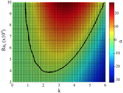
Figure 9: Stability analysis. Values of the largest eigenvalue $\sigma$ in the plane of salinity Rayleigh number $Ra_{s}$ and wavevector $k$. In black is the neutral stability curve. Parameters are those in Table 2.

III.5.1 Varying Schmidt and Péclet numbers

The results above were obtained for $Pe=0.2$ and $Sc=1000$. When $Sc=1$, the neutral stability curve does not change with respect to the one with $Sc=1000$, but the eigenvalues are different. This result is also obtained in the Rayleigh-Bénard instability, in which case it is possible to demonstrate analytically that the Schmidt number does not affect the condition for stability but it does affect the magnitude of the eigenvalues Drazin1981 . Conversely, and as shown in Fig. 10, a higher Péclet number has the effect of lowering the critical Rayleigh number as well making the neutral stability curve broader. These results are expected from the definition of the Péclet number $Pe=h_{0}v_{e}/D$. A higher value can be achieved for example by increasing the evaporation rate, which increases the salt accumulation at the top. From the plots in Fig. 10 one can see that a higher Péclet number also has the effect of increasing the value of the largest eigenvalue, which results in the instability appearing sooner.

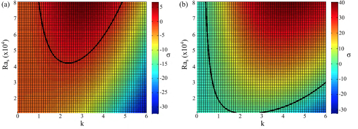
Figure 10: Effect of Péclet number on the neutral stability curve. (a) $Pe=0.1$ and $Sc=1$, (b) $Pe=0.4$ and $Sc=1$.

III.5.2 Varying the time at which the base state is calculated: $t_{0}$

All the results shown above were obtained by considering that the base state is reached within one hour, independent of the initial salt concentration; the salt profile has been calculated according to Eq. (14) and evaluated at time $t_{0}$ (=1 hour). As the dimensionless height was assumed to be constant in the linearized equations $H(t_{0})=H_{0}$, the choice of $t_{0}$ also affects the value of $H_{0}$. Nevertheless, the evaporation speed is so small that the height decreases only $1$ mm in $10$ hours.

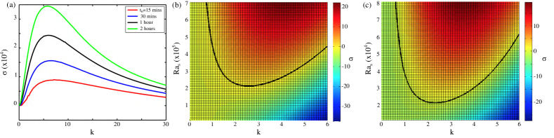
Figure 11: Effects of varying $t_{0}$. (a) Largest eigenvalue for different choices of $t_{0}$, with $Pe=0.2$ and $Ra_{s}=6.6\times 10^{7}$. Neutral stability curves for $t_{0}=15$ min. (b) and $t_{0}=2$ hours (c), both with $Sc=1$ and $Pe=0.2$.

Figure 11a shows the largest eigenvalue $\sigma$ as a function of $k$ when the be state is calculated after $15$ min., $30$ min., $1$ hour and $2$ hours. As expected, the longer one waits, the more salt has accumulated at the top, and the faster the convection starts. Nevertheless the position of the peak remains almost the same, so the wavelength of the pattern is not significantly dependent of the choice of $t_{0}$. Similarly, the largest eigenvalues changes for different values of $t_{0}$. Figure 11 shows the neutral stability curve for (b) $t_{0}=15$ minutes and (c) at $t_{0}=2$ hours. Comparing these figures to Fig. 9 (for $t_{0}=1$ hour) one observes that the choice of $t_{0}$ modifies the value of the critical salinity Rayleigh number without changing the critical wavelength significantly.

IV Two-dimensional finite element studies

The formation of plumes was further investigated by performing numerical simulation in the two-dimensional geometry sketched in Fig. 12. As in the experiments, the initial height of the column of water is $h_{0}$= 1 cm, the length of the cuvette is 6 cm, and the salt concentration is initially homogeneous and equal to $c_{0}$.

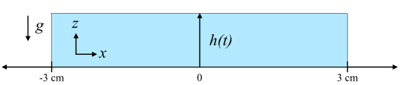
Figure 12: Geometry for full numerical studies. The Navier-Stokes equations are solved in this two-dimensional geometry, with dimensions indicated, $g$ the acceleration of gravity and the height $h(t)$ decreasing in time due to evaporation.

The numerical studies were performed using the finite element package Comsol Multiphysics. In this case, the Navier Stokes equation for the fluid was coupled to the advection-diffusion equation for the salt concentration, as in previous sections. The program was benchmarked on the traditional Rayleigh-Bénard convection with solid-solid boundaries, obtaining a critical Rayligh number of  1700, in good agreement with the known result of 1707.7 Drazin1981 . Comsol can handle the moving top boundary due to evaporation by use of the “Deformable Geometry” module, which works as follows : The equations for the fluid flow and salt concentration are written considering a fixed height $h_{0}$, and an equation for the movement of the top boundary is specified. The code then calculates a new mesh by propagating the deformation throughout the domain. Material is added or removed depending on the movement of the boundaries, thus the total concentration of species is not conserved between iterations Comsol . As in our case the total amount of salt must be conserved, a flux of salt is added at the top.

For the numerical computations, Equations (3) and (4b)-(4a) are rescaled using the following expressions for length, time, flow speed, pressure and salt concentration:

$${\bf x}=\frac{{\bf x}^{*}}{h_{0}},\hskip 14.22636ptt=\frac{D}{h_{0}^{2}}t^{*};\hskip 14.22636pt{\bf u}=\frac{h_{0}}{D}{\bf u}^{*},\hskip 14.22636ptp=\frac{h_{0}^{2}}{\rho_{0}D^{2}}p^{*},\hskip 14.22636ptc=\frac{c^{*}}{c_{0}}.$$

The dimensionless equations to be solved numerically are then

$$\nabla\cdot{\bf u} =0,$$ (29a)

$$\frac{\partial{\bf u}}{\partial t}+{\bf u}\cdot{\bf\nabla}{\bf u} =-\nabla p+Sc\nabla^{2}{\bf u}-RaSc(c-1){\bf\hat{z}},$$ (29b)

$$\frac{\partial c}{\partial t}+{\bf u}\cdot\nabla c =\nabla^{2}c.$$ (29c)

IV.1 Numerical implementation

The boundary conditions for the fluid were non-slip at the lateral and bottom sides, and force-free at the top boundary. The buoyancy force due to the salt concentration was implemented using the “Volume Force” feature of Comsol. The boundary conditions for the salt concentration were no-flux in the lateral and bottom sides. As stated earlier, when a salty suspension evaporates, water leaves the system, but the salt concentration at the top surface increases as this component is conserved in time. This was implemented in Comsol by adding a flux of salt at that the top boundary, which was given by $v_{e}c$, where $v_{e}$ is the dimensionless rate of evaporation (measured experimentally) and $c$ is the dimensionless salt concentration at the top surface. The mesh used was the predefine normal mesh calibrated for fluid dynamics, with a maximum element size 0.045 and minimum element size 0.002. In addition, a corner refinement was added in such way that the elements at the boundaries are scaled by a factor 0.25. The numerical values for the parameters in the simulations are the ones shown in Table 2.

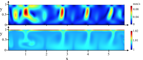
Figure 13: Numerical results for 1% (w/w) initial salt concentration and 60 minutes after the experiment has started. (top) flow field; (bottom) normalized salt concentration.

IV.2 Results

Figure 13 shows the numerical results for experiments with 1% (w/w) salt concentration. The flow speed (in mm/s) and the salt concentration (normalized by its initial value) are shown 60 minutes after the experiment had started. Here one can see the correspondence between high concentrations of salt and the position of the plumes. These numerics also show the rich plume dynamics noticed in the experiments (see Supplemental videos $4$ and $5$ suppl ). In both cases the number of plumes is not constant and coalescence events are observed. The average distance between plumes can be calculated from these images using a similar code to the one described in section II, using the color-coding of the velocity field to identify plumes. After the image was cropped to narrow it in the vertical direction, it was converted to black and white with a threshold of 0.2, and the pixels were averaged vertically. This analysis gives a separation between plumes, averaged over time, for 1% (w/w) salt concentration of $\lambda_{sim,1\%}=0.83\pm 0.17\mbox{ cm}$.

In the experiments it was clear that the lower the overall salt concentration, the longer it takes for plumes to develop, which can be understood from the fact that a longer time is needed to accumulate sufficient salt at the top boundary. As can be seen in Fig. 14, the same feature is observed in the simulations. Here, the snapshots were taken when the plumes first developed, which is longer as the initial salt concentration decreases. In addition, the flow field magnitude also decreases with lower initial salt concentrations. In particular, using $0.001$% (w/w) initial salt concentration, we obtain a typical plume speed of $10^{-4}$ $\mu$m/s, too small to be measured experimentally.

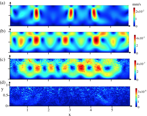
Figure 14: Numerical flow fields for different initial salt concentrations. Snapshots at times corresponding to appearance of plumes for (a) $0.1$% at $t=45$ min., (b) $0.01$% at $t=120$ min, (c) $0.001$% at $t=80$ min, and (d) $0.0001$% at ten hours, at which point no plumes were observed.

V Comparison between experiments, linear stability analysis and numerical simulations

In this section we summarize some of the quantitative measurements of plume obtained using the three approaches. We recall that in the linear stability analysis an infinite two dimensional system was considered, while in the experiments and numerical simulations the system was laterally finite, so geometric confinement effects can occur. Moreover, in the experiments, the cuvette of course had front and back glass walls, so that the dynamics might be considered more like Hele-Shaw flow that a true two-dimensional system.

Separation between plumes. For 1% salt concentration experiments, the time-average over several plumes gave a distance between plumes of $\lambda_{exp,1\%}=0.67\pm 0.06\mbox{ cm}$. From the linear stability analysis, a separation of $\lambda_{linear}=1.05$ cm was obtained, and for the same salt concentration, full non-linear numerical simulations gave $\lambda_{sim,1\%}=0.83\pm 0.17$ cm. In addition, the linear stability analysis gives information about the distance between plumes at the onset of the instability, which can be compared with experimental results before the plumes fully develop. For an initial salt concentration of 0.1% (w/w), the approximate initial separation between plumes is $\lambda_{exp,0.1\%}=1.58\pm 0.08$ cm, which compares very well to the value given by the linear stability analysis of $\lambda_{linear,0.1\%}=1.43\mbox{ cm}$.

Minimal salt concentration needed to observe plumes. In the experiments, the lowest salt concentration for which we could identify a wavelength was $10^{-2}$% (w/w). On the other hand, the linear stability analysis predicts that the critical salt concentration is $5\times 10^{-4}$ % (w/w). This discrepancy can be due to multiple factors, including, as mentioned above, the presence of lateral walls and the added viscous drag associated with the experimental Hele-Shaw geometry. In the numerical simulations, as shown in Fig. 14, no plumes were observed for a salt concentration of $10^{-4}$% (w/w), while for $10^{-3}$% (w/w), very slow plumes can be identified. Therefore, from this approach we obtained that the critical salt concentration is in between $10^{-3}\mbox{ and }10^{-4}$% (w/w), which is in very good agreement with the linear stability analysis result.

Time required to observe plumes. Experimental observations indicate that when using 1% (w/w) salt concentration, the instability developed within $15$ minutes, while for $0.1$% (w/w) plumes appeared $2$ hours after the experiment had started. In a conventional linear stability analysis, the time needed for the instability to start is reflected in the value of the largest eigenvalue, but the in present case there is also the need to wait a sufficient time for evaporation to create a substantial density stratification. Nevertheless, we found that the largest eigenvalue for 1% (w/w) salt was $7$ times larger than for 0.1% (w/w), remarkably close to the experimental ratio of approximately $8$. Similarly, in the numerical simulations with $1$% salt, plumes were observable within $15$ minutes while $45$ minutes were needed to identify plumes in suspensions with $0.1$% salt.

VI Conclusions

We have proposed that accumulation of salt due to evaporation can explain the convective patterns observed in suspensions of a non-motile marine bacterium. This hypothesis was studied using experimental approaches involving control experiments with microspheres of various sizes suspended in growth media with varying salinity. A mathematical model similar in spirit to that used for bioconvection was developed, but focusing on the salt flux created by evaporation at the suspension’s upper surface, and was studied by linear stability analysis and fully nonlinear numerical simulations. The key dimensionless quantity in the model is the salinity Rayleigh number, the critical value of which corresponds to the the threshold of salt concentration needed to observe plumes and determines the wavelength at the onset of the instability. Both results compare well with experimental observations. Similarly, finite-element method simulations showed a plume dynamics very similar to experimental observations, and the dependence on the salt concentration is in agreement with the results obtained using the other two methods.

The phenomenon of interest here was discovered in a suspension of non-motile marine bacteria, but plumes were also observed using a non-marine bacterium (Serratia) with low salt concentration in the medium. Therefore the convection does not require salt in particular, but merely some component that accumulates due to evaporation. The accumulation of solute is always present in experiments with an open-to-air surface, and this effect may have been underestimated in other systems. For the bacterial medium used, the patterns appeared within $15$ minutes, which may certainly be comparable to the duration of typical laboratory experiments. On the other hand, when using motile bacteria, the directed movement (chemotaxis) of cells toward the suspension-air interface is likely to be much stronger than the convection created by solute accumulation Tuval2005 .

In the ocean, an accumulation of salt can generate “salt fingers”, which are formed when cold fresh water surrounds warm salty water. This phenomenon is explained by the fact that thermal diffusion is faster than the salt diffusion, which has the consequence that a region high in salt will cool before the salt can diffuse, creating a descending plume of dense salty water Schmitt1994 . In the ocean this instability has a profound effect on mixing, which influences factors such as the availability of nutrients, heat storage, dispersal of pollutants and the fixation of carbon dioxide, to mention only some effects Huppert1981 . An analogy between the convection in the ocean and the fluid flow observed in a suspension of non-motile P. phosphoreumis particularly interesting, as one could argue that the motion created by evaporation may enhance nutrient mixing. The possibility that bioconvective enhancement of mixing may improve population-level growth has been considered previously and found not to occur Janosi2002 . The relevance of a mixing effect on microorganisms associated with evaporation remains to be studied quantitatively, as does its effect on the so-called “sea surface microlayer”, the submillimeter interfacial layer within which much important geobiochemistry occurs ssmicrolayer .

References

- (1) J. J. Farmer III and F. W. Hickman-Brenner, The Genera Vibrio and Photobacterium, Prokaryotes 6, 508 (2006).
- (2) P. Dunlap and K. Kita-tsukamoto, Luminous Bacteria, Prokaryotes 2, 863-892 (2006).
- (3) T. Pedley and J. O. Kessler, Hydrodynamic Phenomena In Suspensions Of Swimming Microorganisms, Annu. Rev. Fluid Mech. 24, 313 (1992).
- (4) A. J. Pons, F. Sague, M. A. Bees, and P. G. Sorensen, Pattern Formation in the Methylene-Blue-Glucose System, J. Phys. Chem. B 104, 2251 (2000).
- (5) M. R. Benoit, R. B. Brown, P. Todd, E. S. Nelson, and D. M. Klaus, Buoyant plumes from solute gradients generated by non-motile Escherichia coli, Phys. Biol. 5, 1 (2008).
- (6) K. H. Kang, H. C. Lim, H. W. Lee, and S. J. Lee, Evaporation-induced saline Rayleigh convection inside a colloidal droplet, Phys. Fluids 25, 042001 (2013).
- (7) R. Brown, XXIV. Additional remarks on active molecules, Phil. Mag. Ser. 2 6, 161 (1829).
- (8) R. D. Deegan, O. Bakajin, T. F. Dupont, G. Huber, S. R. Nagel, and T. A. Witten, Capillary flow as the cause of ring stains from dried liquid drops, Nature 389, 827 (1997).
- (9) Lord Rayleigh, On convection currents in a horizontal layer of fluid, when the higher temperature is on the under side, Lond., Edin., Dublin Phil. Mag. J. Science 32, 529 (1916).
- (10) O. P. Singh and J. Srinivasan, Effect of Rayleigh numbers on the evolution of double-diffusive salt fingers, Phys. Fluids 26, 062104 (2014).
- (11) R. A. Wooding, S. W. Tyler, and I. White, Convection in groundwater below an evaporating Salt Lake: 2. Evolution of fingers or plumes, Water Res. Research 33, 1219 (1997).
- (12) See Supplemental information available at XXX for videos of experimental results and numerical studies.
- (13) H. Bénard, Les tourbillons cellulaires dans une nappe liquide, J. Phys. Th. App. 10, 254 (1901).
- (14) Y. Renardy and R. Schmitt, Linear stability analysis of salt fingers with surface evaporation or warming, Phys. Fluids 8, 2855 (1996).
- (15) L. F. Shampine and J. Kierzenka, pdepe for Matlab. http://uk.mathworks.com/help/matlab/ref/pdepe.html (2005).
- (16) P. G. Drazin, and W. H. Reid, Hydrodynamic Stability, Cambridge University Press, 2nd edition (2004).
- (17) Comsol Mutiphysics Reference Manual, version 5.0 (2014).
- (18) R. Schmitt, Double Diffusion in Oceanography, Annu. Rev. Fluid Mech. 26, 255 (1994).
- (19) I. Tuval, L. Cisneros, C. Dombrowski, C. W. Wolgemuth, J. O. Kessler, and R. E. Goldstein, Bacterial swimming and oxygen transport near contact lines, Proc. Natl. Acad. Sci. USA 102, 2277 (2005).
- (20) H. E. Huppert and J. S. Turner, Double-Diffusive Convection, J. Fluid Mech. 106, 299 (1981).
- (21) I. M. Jánosi, A. Czirók, D. Silhavy, and A. Holczinger, Is bioconvection enhancing bacterial growth in quiescent environments?, Env. Microbiology 4, 525 (2002).
- (22) M. Cunliffe, et al., Sea surface microlayers: a unified physicochemical and biological perspective of the air-ocean interface, Prog. Ocean. 109, 104 (2013).