Phase limitations of Zames-Falb multipliers

Abstract

Phase limitations of both continuous-time and discrete-time Zames-Falb multipliers and their relation with the Kalman conjecture are analysed. A phase limitation for continuous-time multipliers given by Megretski is generalised and its applicability is clarified; its relation to the Kalman conjecture is illustrated with a classical example from the literature. It is demonstrated that there exist fourth-order plants where the existence of a suitable Zames-Falb multiplier can be discarded and for which simulations show unstable behavior. A novel phase-limitation for discrete-time Zames-Falb multipliers is developed. Its application is demonstrated with a second-order counterexample to the Kalman conjecture. Finally, the discrete-time limitation is used to show that there can be no direct counterpart of the off-axis circle criterion in the discrete-time domain.

I Introduction

The absolute stability of a negative feedback interconnection between an LTI system $G$ and a nonlinearity $\phi$ with a slope restriction $k$ has aroused the interests of many researchers. The stability tests include the circle criterion, Popov criterion [1], [2], and off-axis circle criterion [3], [4] in continuous time and the circle criterion [5], Tsypkin criterion [6] and Jury-Lee criterion [7], [8] in discrete time. For a recent discussion, see [9] and [10]. Apart from these, loop transformation and multiplier theory are both important tools to establish the stability of feedback interconnections. The Zames-Falb multipliers are a class of multipliers with the property of preserving the positivity of monotone and bounded nonlinearities, and hence of slope-restricted nonlinearities after loop transformation. The class of Zames-Falb multipliers can be defined in either continuous time [11, 12] or discrete time [13, 14]. Specifically, after loop transformation, the stability of the negative interconnection between an LTI system $G$ and a nonlinearity $\phi$ with a slope restriction $k$ is guaranteed if there exists a Zames-Falb multiplier $M$ such that

$$\mbox{Re}\{M(1+kG)\}>0,$$ (1)

with $M$ and $G$ evaluated over all frequencies. That is to say, at $j\omega$, $\omega\in\mathds{R}$ for continuous-time systems and at $e^{j\omega}$, $\omega\in[0,2\pi]$ for discrete-time systems.

The Zames-Falb multipliers may be considered a classical tool [15]. Nevertheless, there has been considerable recent interest, largely sparked by the availability of numerical searches ([16], [17], [18], [19], [20], [21], [22], for continuous time; [23], [24] for discrete time) and their encapsulation within an IQC (integral quadratic constraint) framework [25], [26], [27], [28]. There has also been interest in generalising the class, both to MIMO (multi-input, multi-output) nonlinearities [29], [30], [31], [32], [33] and to nonlinearities outside the original classes considered by Zames and Falb [34], [35], [28], [36]. In addition to determining stability conditions, they can be used to analyse performance [37], [38]; further, they can be used to obtain tighter versions of the Popov criterion [39]. Applications of Zames-Falb multipliers range from input-constrained model predictive control [40] to first order numerical optimisation algorithms [41].

TABLE I: Various slope restrictions discussed in the text.

$\hat{k}_{ZF}$	Maximum slope for which a Zames-Falb multiplier is known
$k_{ZF}$	Maximum slope for which there exists a Zames-Falb multiplier
$k_{S}$	Maximum slope for which the Lur’e system is absolutely stable
$k_{PL}$	Minimum slope for which phase limitation implies there is no
	Zames-Falb multiplier
$\hat{k}_{C}$	Minimum slope for which a counterexample to absolute
	stability is known
$k_{O}$	Slope for direct discrete-time counterpart off-axis circle criterion
	(which is false)
$k_{RO}$	Slope for Reduced Off-axis circle criterion in [42]
$k_{N}$	Nyquist value

Figure 1: Relations between slope restrictions discussed in the text. Conjecture I.2 is that $k_{ZF}=k_{S}$ and hence $k_{S}<k_{PL}$.

Figure 2: Lur’e problem

Although both continuous-time and discrete-time Zames-Falb multipliers are defined with similar conditions, there are clear distinctions between their properties. In discrete time the Zames-Falb multipliers are the full set of multipliers preserving the positivity of monotone and bounded nonlinearities, besides direct phase substitutions [14], [43]. In continuous time matters are more nuanced, but the class of Zames-Falb multipliers remains the widest known class of multipliers preserving the positivitiy of monotone and bounded nonlinearities, up to phase equivalence [39, 44]. For a tutorial introduction to the phase properties of continuous-time Zames-Falb multipliers, phase-equivalence results and the issues associated with causality, see [45]. Phase properties are essential to our understanding of Zames-Falb multipliers.

For example, if $k<k_{N}$ (see Table I for various slope restrictions discussed in this paper), then the phase of $(1+kG)$ lies between $-180^{\circ}$ and $180^{\circ}$. Meanwhile multipliers must be positive so are restricted to lie between $-90^{\circ}$ and $90^{\circ}$. But as the Kalman conjecture is false, any set of suitable multipliers must be restricted by some further fundamental limitations. This follows from the obvious but important fact:

Fact I.1.

If the system is not absolutely stable, there can be no appropriate Zames-Falb multiplier.

However, only a few papers discuss such limitations. Megretski [46] shows that there exists a phase limitation for continuous-time Zames-Falb multipliers. Another phase limitation of Zames-Falb multipliers is given by Jönsson and Laiou [47, 48]. Such limitations are often ignored when new searches for multipliers are presented (see for example [45] and references therein). Often only $k_{N}$ is provided as an upper limit for the slope restriction.

We discuss Megretski’s phase restriction [46] with respect to a fourth-order continuous-time plant whose phase drops from $+180^{\circ}$ to $-180^{\circ}$; similarly with $k$ sufficiently big the phase of $1+kG$ drops from above $+90^{\circ}$ degrees to below $-90^{\circ}$. The limitation cannot be applied to first, second or third-order plants whose phase is in the range $(-180,90)$ degrees or $(-90,180)$ degrees; this agrees with the well-known result that the Kalman conjecture is true for such plants [49].

To the best of authors’ knowledge, no similar limitation has been developed in the discrete-time domain. Since there exist second-order discrete-time counterexamples to the Kalman conjecture whose phase is in the range $(-180,0)$ degrees [50, 51] one might expect a simpler limitation for discrete-time multipliers; this turns out to be indeed the case.

The contribution of this paper is for both continuous-time and discrete-time multipliers. We generalise Megretski’s limitation [46] for continuous-time multipliers to a wider choice of frequency intervals. Further, we show that Megrestki’s limitation [46] only applies for the class of Zames-Falb multipliers which do not require the odd condition on the nonlinearity; we provide the corresponding result when the nonliearity is odd. We discuss the limitation’s numerical calculation and demonstrate its application in the context of a classical example due to O’Shea [11, 45]. In particular we demonstrate a fourth-order counterexample of the Kalman conjecture for which the constraint is active. A further contribution of the paper is the development of a phase limitation for discrete-time Zames-Falb multipliers. This limitation is fundamentally different to Megrestki’s limitation as it only requires the phase of $(1+kG)$ to be either in the interval $(90,180)$ degrees or in the interval $(-180,-90)$ degrees. The limitation is easy to compute, and is active for a second-order discrete-time counterexample of the Kalman conjecture. This close link between the preclusion of a Zames-Falb multiplier and unstable behaviour leads us to the following conjecture as the counterpart to Fact I.1; however no proof (or counterexample) is offered in this paper:

Conjecture I.2.

If there is no appropriate Zames-Falb multiplier, the system is not absolutely stable.

One direct application of the phase limitation is to show there can be no direct discrete-time counterpart of the off-axis circle criterion. The continuous-time off-axis circle criterion is a useful graphical stability test and is shown to be a less conservative criterion compared to the circle criterion [3], [4]. The derivation is based on the phase properties of RL/RC multipliers. The direct discrete-time counterpart of the off-axis circle criterion is sometimes assumed to be true in the literature (e.g. [52], [53]). However only a highly restrictive discrete-time version is proposed in [42], without discussion as to whether the direct discrete-time counterpart off-axis circle criterion is true or false. In this paper, we show that in some cases there are no Zames-Falb multipliers with the requisite phase properties for its derivation - i.e. the direct counterpart off-axis circle criterion cannot be derived using multiplier theory. The invalidation is completed by counterexample.

Some preliminary results related with Theorem IV.3 part (i) were presented in [54].

II Notation and Preliminary results

II-A Signal spaces

For continuous-time signals let $\mathcal{L}_{2}[0,\infty)$ be the Hilbert space of square integrable and Lebesgue measurable functions $f:[0,\infty)\rightarrow\mathds{R}$ and let $\mathcal{L}_{2}$ be defined similarly for $f:\mathds{R}\rightarrow\mathds{R}$. Let $\mathcal{L}_{2e}[0,\infty)$ be the extended space of $\mathcal{L}_{2}[0,\infty)$ [43].

For discrete-time signals let $\mathds{Z}$ and $\mathds{Z^{+}}$ be the set of integer numbers and positive integer numbers including $0$, respectively. Let $\ell$ be the space of all real-valued sequences, $h:\mathds{Z}^{+}\rightarrow\mathds{R}$ and let $\ell_{2}$ denote the Hilbert space of all square-summable and measurable real sequences $f:\mathds{Z}^{+}\rightarrow\mathds{R}$ ($\ell$ is the extended space of $\ell_{2}$). Similarly, we can define the Hilbert space $\ell_{2}(\mathds{Z})$ by considering real sequences $f:\mathds{Z}\rightarrow\mathds{R}$.

II-B Lur’e problem and the Kalman conjecture

The feedback interconnection system is a Lur’e system represented in Fig. 2 with both $G$ and $\phi$ mapping $\mathcal{L}_{2e}[0,\infty)\rightarrow\mathcal{L}_{2e}[0,\infty)$ (continuous time) or $\ell\rightarrow\ell$ (discrete time). The object $G$ is assumed LTI stable and the object $\phi$ memoryless and slope-restricted (see below). The interconnection relationship is

$$\begin{cases}v=f+Gw,&\\ w=-(\phi v)+g.&\end{cases}$$ (2)

The system (2) is well-posed if the map $(v,w)\mapsto(g,f)$ has a causal inverse on $\ell\times\ell$, and this feedback interconnection is $\ell_{2}$-stable if for any $f,g\in\ell_{2}$, both $w,v\in\ell_{2}$.

Definition II.1.

(Memoryless slope-restricted nonlinearity) The nonlinearity $\phi:\mathcal{L}_{2e}[0,\infty)\rightarrow\mathcal{L}_{2e}[0,\infty)$ or $\phi:\ell\rightarrow\ell$ is said to be memoryless and slope-restricted in $S[0,k]$, if there is a function $N:\mathds{R}\rightarrow\mathds{R}$ such that $(\phi u)(t)=N(u(t))$ or $(\phi u)(k)=N(u(k))$, $N(0)=0$, and

$$0\leq\frac{N(x_{1})-N(x_{2})}{x_{1}-x_{2}}\leq k,\quad\forall x_{1},x_{2}\in\mathds{R},x_{1}\neq x_{2}.$$ (3)

In addition, $\phi$ is said to be odd if $N$ is odd, i.e. $N(x)=-N(-x)$, for all $x\in\mathds{R}$.

We define the Nyquist value and state the Kalman conjecture for both continuous-time and discrete-time systems.

Definition II.2 (Nyquist value).

Given a stable LTI system $G$, the Nyquist value $k_{N}$ is the supremum of all the positive real numbers $k$ such that $\tau kG$ satisfies the Nyquist Criterion for all $\tau\in[0,1]$. It can also be expressed as:

$$k_{N}=\sup\{k>0:\inf_{\omega}\{|1+\tau kG|\}>0),\forall\tau\in[0,1]\},$$ (4)

with $G$ evaluated over all frequencies (i.e. $\omega\in\mathbb{R}$ for continuous-time systems and $\omega\in[0,2\pi]$ for discrete-time systems).

Conjecture II.3 (Kalman Conjecture, [55]).

Let $\phi$ be a memoryless slope-restricted nonlinearity such that there exists a continuously differentiable $N:\mathds{R}\rightarrow\mathds{R}$ and $S>0$ such that $\phi(v)(t)=N(v(t))$ (or $\phi(v)(k)=N(v(k))$) and

$$0\leq\frac{dN(x)}{dx}\leq S,\quad\forall x\in\mathds{R}.$$ (5)

Then the negative feedback interconnection of the continuous-time (or discrete-time) LTI systems $G\sim[A,B,C,0]$ and $\phi$ (Fig 2) is globally asymptotically stable if $A-BCk$ is Hurwitz (Schur) for all $k\in[0,S]$.

There exist fourth-order continuous-time counterexamples to the Kalman conjecture [56, 49, 57] and second-order discrete-time counterexamples [50, 51].

II-C Zames-Falb multipliers

The characteristics of continuous-time Zames-Falb multipliers is given in the following theorem that defines two different classes of multipliers.

Theorem II.4.

(Continuous-time Zames-Falb multipliers, [12].) Consider the continuous-time feedback system in Fig. 2 with $G$ a stable LTI system and $\phi$ memoryless and slope-restricted in $S[0,k]$. Suppose that there exists an LTI multiplier $M:\mathcal{L}_{2}\rightarrow\mathcal{L}_{2}$ whose transfer function has the form

$$M(s)=1-H(s)$$ (6)

such that the impulse response $h$ of $H$ satisfies

$$\int_{-\infty}^{\infty}|h(t)|\,dt<1.$$ (7)

Moreover, let us assume that either $\phi$ is odd or $h(t)>0$. Suppose further there is some $\delta>0$ such that

$$\mbox{Re}\left\{M(j\omega)(1+kG(j\omega))\right\}\geq\delta\mbox{ for all }\omega\in\mathbb{R}.$$ (8)

Then the feedback interconnection (2) is $\mathcal{L}_{2}$-stable.  ∎

Remark II.5.

With some abuse of notation, we denote $h(t)$ as the addition of a real-valued function $h_{a}(t)$ and impulses at different instants, i.e.

$$h(t)=h_{a}(t)+\sum_{i=1}^{\infty}h_{i}\delta(t_{i}).$$ (9)

Definition II.6.

The class of continuous-time Zames-Falb multipliers $\mathcal{M}^{c}$ is defined as the LTI systems $M:\mathcal{L}_{2}\rightarrow\mathcal{L}_{2}$ whose transfer function has the form

$$M(s)=1-H(s)$$ (10)

such that the impulse response $h$ of $H$ satisfies that $h(t)\geq 0$ for all $t$ and

$$\int_{-\infty}^{\infty}h(t)\,dt<1.$$ (11)

Definition II.7.

The class of continuous-time “odd” Zames-Falb multipliers $\mathcal{M}^{c}_{\text{odd}}$ is defined as the LTI systems $M:\mathcal{L}_{2}\rightarrow\mathcal{L}_{2}$ whose transfer function has the form

$$M(s)=1-H(s)$$ (12)

such that the impulse response $h$ of $H$ satisfies

$$\int_{-\infty}^{\infty}|h(t)|\,dt<1.$$ (13)

By definition, $\mathcal{M}^{c}\subset\mathcal{M}^{c}_{\text{odd}}$.

The counterpart result in discrete time is given in the following theorem and it also defines two different classes of multipliers:

Theorem II.8.

(Discrete-time Zames-Falb multipliers, [14], [43]) Consider the discrete-time feedback system in Fig. 2 with $G$ a stable LTI system and $\phi$ memoryless and slope-restricted in $S[0,k]$. Suppose that there exists an LTI multiplier $M:\ell_{2}\rightarrow\ell_{2}$ whose transfer function has the form

$$M(z)=1-H(z)$$ (14)

such that the impulse response $h$ of $H$ satisfies that $h_{0}=0$ and

$$\sum_{i=-\infty}^{\infty}|h_{i}|<1.$$ (15)

Moreover, let us assume that either the nonlinearity is odd or $h_{i}\geq 0$. Suppose further

$$\hbox{Re}\left\{M(z)(1+kG(z))\right\}>0,\quad\forall|z|=1.$$ (16)

Then the feedback interconnection (2) is $\ell_{2}$-stable.  ∎

Remark II.9.

Inequality (8) is evaluated over $\omega\in\mathbb{R}$ whereas inequality (16) is evaluated over the frequency interval $\omega\in[0,2\pi]$. Hence, by the Extreme Value Theorem [58], it is unnecessary to define any $\delta>0$ for the discrete case corresponding to that used in the continuous case.

Similarly to the previous definitions, we can define the classes of multipliers $\mathcal{M}^{d}$ and $\mathcal{M}^{d}_{\text{odd}}$.

II-D Off-axis circle criterion

The continuous-time off-axis circle criterion is given.

Lemma II.10.

(Off-axis circle criterion for continuous-time
systems, [3]) Consider the feedback system in Fig. 2 with $G$ LTI stable and $\phi$ is slope-restricted in $S[0,k]$. Suppose that the Nyquist plot of the linear part of the system $G(j\omega)$ lies entirely to the right of a straight line passing through the point $(-\frac{1}{k}+\delta,0)$ where $\delta>0$ and $\phi$ is monotonically increasing. Then the feedback interconnection (2) is $\mathcal{L}_{2}$-stable.

For discrete time, only a highly restrictive version is proposed.

Lemma II.11.

(Reduced off-axis circle criterion for discrete-time systems, [42]) Let the Nyquist plot of $G(e^{j\omega})$ for all $0\leq\omega\leq\pi$ lie entirely to the right of a straight line, whose slope $k$ is nonnegative passing through $(-\frac{1}{K_{2}},0)$. Let $\omega_{0}$ be such that $\mbox{Re }G(e^{j\omega_{0}})=-\frac{1}{K_{2}}$ and $\mbox{Re }G(e^{j\omega})\geq-\frac{1}{K_{2}}$ for $\omega\geq\omega_{0}$ and $\mbox{Im }G(e^{j\omega})\leq 0$ for $\omega_{0}\geq\omega\geq 0$. Then the system is asymptotically stable for all monotone $\phi$ with slope restriction $K_{2}$ in the feedback path if

$$\theta\leq-\frac{1}{2}\omega_{0}+\frac{\pi}{2},$$ (17)

where $\theta$ is the angle made by the straight line and the imaginary axis, i.e., $\theta=\cot^{-1}k$. If $\mbox{Im }G(e^{j\omega})\geq 0$ for $\omega_{0}\geq\omega\geq 0$, the same argument can be used to prove the asymptotic stability of the system with nonpositive $k$ and

$$\theta\geq\frac{1}{2}\omega_{0}-\frac{\pi}{2}.$$ (18)

II-E Further mathematical notation

For the convenience of solving potential numerical issues, the notation of $O(\cdot)$ is given.

Definition II.12.

The condition

$$f(t)=g(t)+O(t^{n}),\mbox{ as }t\rightarrow 0.$$ (19)

means that there exist $M$ and $t_{0}$ such that

$$|f(t)-g(t)|\leq Mt^{n}\mbox{ on }[0,t_{0}].$$ (20)

The floor function, denoted by $\lfloor\nu\rfloor$, is defined by

$$\lfloor\nu\rfloor=\max\{m\in\mathbb{Z}\mid m\leq\nu\}.$$ (21)

III Continuous phase limitations and the Kalman conjecture

Megretski presents in [46] a phase limitation for continuous-time Zames-Falb multipliers. In this section we generalise the result to a wider set of frequency intervals, and derive separate results for both $\mathcal{M}^{c}$ and $\mathcal{M}^{c}_{odd}$. Although it is stated in [46] that the result there is valid for $\mathcal{M}^{c}_{odd}$ (in the terminology of this paper) we show by counterexample that it is in fact valid for $\mathcal{M}^{c}$ only. Finally, we bridge the limitation of [46] with the Kalman conjecture; this is the key motivation to develop a different set of phase limitations for the discrete-time Zames-Falb multipliers.

III-A Phase limitations

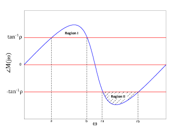
Figure 3: Illustration of Theorem III.4 with the choice of interval from [46]: $\kappa=1$, $c=ra$ and $d=rb$. The result is given in terms of $\rho$ while the phase of the multiplier $M$ is $\tan^{-1}\rho$.

Definition III.1.

Let $0<a<b<c<d$, $\kappa>0$, $\lambda>0$ and $\mu>0$. Define

$$\rho^{c}=\sup_{t>0}\frac{|\psi(t)|}{\phi(t)},$$ (22)

and

$$\rho^{c}_{odd}=\sup_{t>0}\frac{|\psi(t)|}{\tilde{\phi}(t)},$$ (23)

where

$$\psi(t) =\frac{\lambda\cos(at)}{t}-\frac{\lambda\cos(bt)}{t}-\frac{\mu\cos(ct)}{t}+\frac{\mu\cos(dt)}{t},$$ (24)

$$\phi(t) =\lambda(b-a)+\kappa\mu(d-c)+\phi_{1}(t),$$ (25)

and

$$\tilde{\phi}(t) =\lambda(b-a)+\kappa\mu(d-c)-|\phi_{1}(t)|,$$ (26)

with

$$\phi_{1}(t)=\frac{\lambda\sin(at)}{t}-\frac{\lambda\sin(bt)}{t}+\frac{\kappa\mu\sin(ct)}{t}-\frac{\kappa\mu\sin(dt)}{t}.$$ (27)

Lemma III.2.

If $\lambda$ and $\mu$ are chosen such that

$$\frac{\lambda}{\mu}=\frac{d^{2}-c^{2}}{b^{2}-a^{2}},$$ (28)

then $\rho^{c}$ and $\rho^{c}_{odd}$ in Definition III.1 are well-defined; that is to say $\rho^{c}<\infty$ and $\rho^{c}_{odd}<\infty$.

Proof:

See Appendix.

Remark III.3.

The direct calculation of the ratios $\psi(t)/\phi(t)$ and $\psi(t)/\tilde{\phi}(t)$ is numerically ill-conditioned for small $t$ since, with the choice (28), we have $\psi(t)=0+O(t^{3})$, $\phi(t)=0+O(t^{2})$ and $\tilde{\phi}(t)=0+O(t^{2})$, all as $t\rightarrow 0$. Nevertheless, the same construction ensures we can write

$$\frac{\psi(t)}{\phi(t)}=\gamma t+O(t^{3})\mbox{ and }\frac{\psi(t)}{\tilde{\phi}(t)}=\gamma t+O(t^{3})\mbox{ as }t\rightarrow 0,$$ (29)

with

$$\gamma=-\frac{1}{4}\frac{\lambda(b^{4}-a^{4})-\mu(d^{4}-c^{4})}{\lambda(b^{3}-a^{3})+\kappa\mu(d^{3}-c^{3})}.$$ (30)

We use this relation for small $t$ in the numerical examples below.

Theorem III.4 (Continuous-time phase limitations).

Let $M$ be a continuous-time Zames-Falb multiplier. Suppose

$$\mbox{Im}(M(j\omega)) >\rho\mbox{Re}(M(j\omega))\mbox{ for all }\omega\in[a,b],$$ (31)

and

$$\mbox{Im}(M(j\omega)) <-\kappa\rho\mbox{Re}(M(j\omega))\mbox{ for all }\omega\in[c,d],$$ (32)

for some $\rho>0$. Then under the conditions of Lemma III.2.

1. $\rho<\rho^{c}$ if $M\in\mathcal{M}^{c}$,

2. $\rho<\rho^{c}_{odd}$ if $M\in\mathcal{M}^{c}_{odd}$.

Proof:

See Appendix.

Lemma III.2 and Theorem III.4, with the choice $\kappa=1$, $c=ra$, $d=rb$ and hence $\lambda/\mu=r^{2}$, are in [46]. An interpretation of Theorem III.4 with these values is illustrated in Fig. 3 (see also [45]). According to the constraints on the coefficients of continuous Zames-Falb multipliers, if the phase is simultaneously greater than $\tan^{-1}\rho$ on $\omega\in[a,b]$ (in Region I) and smaller than $-\tan^{-1}\rho$ on $\omega\in[ra,rb]$ (in Region II), then $\rho<\rho^{c}$ if $M\in\mathcal{M}^{c}$ and $\rho<\rho^{c}_{odd}$ if $M\in\mathcal{M}^{c}_{odd}$.

Remark III.5.

It is straightforward to produce the counterpart of Theorem III.4 with (31) and (32) replaced by $\mbox{Im}(M(j\omega))<-\rho\mbox{Re}(M(j\omega))$ for all $\omega\in[a,b]$ and $\mbox{Im}(M(j\omega))>\kappa\rho\mbox{Re}(M(j\omega))$ for all $\omega\in[c,d]$ respectively.

Remark III.6.

In [46], Megretski uses a positive sign in the exponential of the Laplace transform:

$$M(j\omega)=1-\int_{-\infty}^{\infty}e^{j\omega t}h(t)dt.$$ (33)

This is the standard convention in the Physics literature (see for example [59]) but opposite to that used in [12]. The apparent discrepancy has no significant consequence for the analysis of phase limitations since if $M(s)$, with impulse response $m(t)$, is a Zames-Falb multiplier then $M(-s)$, with impulse response $m(-t)$, is also a Zames-Falb multiplier.

It is natural to ask whether a phase limitation over a single frequency range can be constructed in a similar manner. This is not possible in continuous time, as any corresponding definition of $\rho^{c}$ or $\rho^{c}_{odd}$ would be unbounded as $t$ approaches $0$. Loosely speaking, we can generate a multiplier in $\mathcal{M}^{c}$ with phase arbitrarially close to $\pm 90^{\circ}$ over an arbitrararily large frequency inteterval by selecting $h(t)=(1-\epsilon)\delta(t-t^{*})$ with $\epsilon>0$ arbitrarially close to $0$ and $t^{*}$ arbitrarially close to 0. But we construct such phase limitations for discrete-time multipliers below, in Section IV.

III-B Numerical example

Here we illustrate Theorem III.4 with a numerical example. Let $a=1.6$ and $b=2.25$. Let $\kappa=1$, $c=ra$ and $d=rb$ with $r=2.1$. Then a sweep over time intervals followed by local numerical search gives

$$\rho^{c}\approx 0.6069\mbox{, }\tan^{-1}\rho^{c}\approx 31.25^{\circ},$$ (34)

and

$$\rho^{c}_{odd}\approx 1.4928\mbox{, }\tan^{-1}\rho^{c}_{odd}\approx 56.18^{\circ}.$$ (35)

Now consider the multiplier

$$M(j\omega)=1-\int_{-\infty}^{\infty}e^{-j\omega t}h(t)dt$$ (36)

with $h(t)=-0.9\delta(t+1)$. Figure 4 shows that the relations (31) and (32), or equivalently

$$\angle M(j\omega)>\tan^{-1}\rho\mbox{ over the interval }[a,b],$$ (37)

and

$$\angle M(j\omega)<-\tan^{-1}\rho\mbox{ over the interval }[ra,rb],$$ (38)

are satisfied simultaneously for $\rho=\rho^{c}$ but not for $\rho=\rho^{c}_{odd}$. This is consistent with Theorem III.4 as $M\in\mathcal{M}^{c}_{odd}$ but $M\notin\mathcal{M}^{c}$. It is a counterexample to the false claim in [46] that the phase limitation of Theorem III.4 part (i) is applicable to the wider class $M\in\mathcal{M}^{c}_{odd}$.

Remark III.7.

Both in this numerical example and at the end of Section III-A we consider multipliers where $h$ takes the form $h(t)=(1-\varepsilon)\delta(t-\tau)$ for some $\tau$. There is a close link with Theorem III.4. Specifically if $|\psi(\tau)|/\phi(\tau)=\rho^{c}$ and $\varepsilon\rightarrow 0$ then

$$\int_{-\infty}^{\infty}\psi(t)h(t)dt=\rho^{c}[\lambda(b-a)+\kappa\mu(d-c)]+\rho^{c}\int_{-\infty}^{\infty}\phi_{1}h(t)\,dt.$$ (39)

Compare (80) in the proof of Theorem III.4. Similarly if $|\psi(\tau)|/\tilde{\phi}(\tau)=\rho^{c}_{odd}$ then

$$\int_{-\infty}^{\infty}\psi(t)h(t)dt=\\ =\rho^{c}_{odd}[\lambda(b-a)+\kappa\mu(d-c)]+\rho^{c}_{odd}\int_{-\infty}^{\infty}\phi_{1}h(t)\,dt.$$ (40)

We discuss the corresponding relations at greater length in Section IV-B for the discrete-time case.

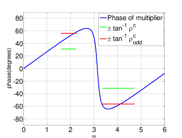
Figure 4: Phase of the multiplier (36) and the continuous phase limitations $\pm\tan^{-1}\rho^{c}\approx\pm 31.25^{\circ}$ and $\pm\tan^{-1}\rho^{c}_{odd}\approx\pm 56.18$ evaluated on $[1.6,2.25]$ and $[3.36,4.725]$.

III-C Counterexamples to Kalman conjecture via phase limitations

It is instructive to interpret the phase limitations of Theorem III.4 in a manner consistent with known results about the Kalman conjecture.

On the one hand, it is well-known that first, second and third order plants hold the Kalman conjecture [49]. The phase of such plants cannot reach both Regions I and II in Fig. 3. So the phase limitations cannot apply to these plants. First-order plants do not require a dynamic multiplier, second-order plants require a dynamics multiplier with a tunable zero and a pole at infinity, i.e. a Popov multiplier, and-third order plant requires both a tunable pole and zero, i.e. first order RL/RC multipliers. In all these cases, only a first-order multiplier is required, and we know that there is no phase limitation in the selection of such multipliers [39].

Remark III.8.

Although the off-axis circle criterion is also based on RL/RC multipliers, it is not sufficient to show all third-order plants hold the Kalman conjecture. For example, the off-axis circle criterion with the plant

$$G=\frac{s^{2}}{s^{3}+1.002s^{2}+s+0.998},$$ (41)

guarantees stability with $k<3.928$, whereas the multiplier $M=(s+1)/(s+\epsilon)$ guarantees stability for any positive $k$ with a sufficiently small value $\epsilon>0$.

On the other hand the phase limitations may be applied to fourth-order plants, and these in turn may be counterexamples to the Kalman conjecture by: a) showing numerically that a phase limitation can be applied to a well-known plant, and b) showing that the Lur’e system with this plant and a slope-restricted nonlinearity may be unstable.

Specifically we will consider the phase limitation of Theorem III.4 part (i) with $\kappa=1$, $c=ra$, and $d=rb$; that is to say the original result of [46] applied to $\mathcal{M}^{c}$. A particularly suitable example to show this limitation is O’Shea example [11, 45]:

$$G(s)=\frac{s^{2}}{(s^{2}+2\xi s+1)^{2}},$$ (42)

since the symmetry of the problem simplifies the selection of the parameters. In this example, O’Shea showed that there is a Zames-Falb multiplier for any $k$ if $\xi>0.5$. The following result shows that it is not possible to reach an arbitrary large $k$ for any $\xi\leq 0.25$. For the case $\xi=0.25$, the phase of $G(s)$ is above $177.98^{\circ}$ over the interval $[a,b]$ where $a=0.02249$ and $b=0.03511$; hence it is below $-177.98^{\circ}$ over the interval $[1/b,1/a]$ by using the symmetry of the plant. Then a suitable Zames-Falb multiplier for this plant would require a phase below $-87.98^{\circ}$ over the interval $[a,b]$ and above $87.98^{\circ}$ over the interval $[1/b,1/a]$. The phase limitation ensures that there is no Zames-Falb multiplier with such a phase characteristic, since $\tan^{-1}\rho^{c}\approx 87.79^{\circ}$. Strictly speaking, we have used the counterpart of Theorem III.4 mentioned in Remark III.5.

Although numerical reliability can be problematic in the discussion of the Kalman conjecture [57], simulations of the plant with asymmetrical saturation show a time evolution that does not appear to settle to zero, supporting the validity of Conjecture I.2. The simulation shown in Figure 5 has been run in MATLAB R2013, using the solver ode45, with maximum step size of 0.0001 s, and relative tolerance of $10^{-3}$. The nonlinearity $\phi$ is described by the nonlinear function

$$N(x)=\begin{cases}-1000&x<-1;\\ 1000x&-1\leq x\leq 0;\\ 0&x>0;\end{cases}$$ (43)

the input $g$ is given by

$$g(t)=\begin{cases}100&t\leq 20\text{s};\\ 0&t>20\text{s};\end{cases}$$ (44)

and $f(t)=0$. The relevance of this counterexample to the Kalman conjecture is that we can show that there is no Zames-Falb multiplier with $h(t)\geq 0$ for the system. The asymmetry of the nonlinearity seems to be a key factor as simulations with symmetric saturations show stable behaviour. The importance of asymmetry in the stability of Lur’e systems with saturation has been discussed recently [36, 60].

Figure 5: Amplitude of the signal $\nu$ in a simulation of the feedback interconnection depicted in Fig. 2 where G is given by (42) with $\xi=0.25$, $\phi$ is described by (43), $g(t)$ is given by (44), and $f(t)=0$.

Remark III.9.

The magnitude of the response in Fig. 5 is bounded. Since the plant $G$ is stable and $\phi$ is sector-bounded it follows that if $g\in\mathcal{L}_{\infty}$ then all signals must be in $\mathcal{L}_{\infty}$.

IV Discrete-time phase limitation

In this section we develop phase limitations for discrete-time Zames-Falb multipliers. Their derivation is in the spirit of Megretski’s limitation [46] and Theorem III.4 for continuous-time multipliers. However their properties are simpler and consistent with the existence of second-order discrete-time counterexamples to the Kalman conjecture [50, 51]. In particular, and by contrast with their continuous-time counterparts, they are concerned with properties over a single interval $\omega\in[a,b]$.

It is worth highlighting that if a discrete-time multiplier preserves the positivity of all monotone and bounded nonlinearities then either it is a Zames-Falb multiplier or there exists a Zames-Falb multiplier with the same phase [14], [43]. Hence any phase limitation on the discrete-time Zames-Falb multipliers is also a limitation for any discrete-time multiplier.

IV-A Phase limitations

Definition IV.1.

Let $0\leq a<b\leq\pi$. Define

$$\rho^{d}=\max_{n\in\mathbb{Z}^{+}}\frac{|\psi_{d}(n)|}{\phi_{d}(n)},$$ (45)

and

$$\rho^{d}_{odd}=\max_{n\in\mathbb{Z}^{+}}\frac{|\psi_{d}(n)|}{\tilde{\phi}_{d}(n)},$$ (46)

where

$$\psi_{d}(n) =\frac{\cos(an)}{n}-\frac{\cos(bn)}{n},$$ (47)

$$\phi_{d}(n) =(b-a)+\phi_{d,1}(n),$$ (48)

and

$$\tilde{\phi}_{d}(n) =(b-a)-|\phi_{d,1}(n)|,$$ (49)

with

$$\phi_{d,1}(n)=\frac{\sin(an)}{n}-\frac{\sin(bn)}{n}.$$ (50)

Lemma IV.2.

Both $\rho^{d}$ and $\rho^{d}_{odd}$ in Definition IV.1 are well-defined; that is to say $\rho^{d}<\infty$ and $\rho^{d}_{odd}<\infty$.

Proof:

See Appendix.

Theorem IV.3 (Discrete-time phase limitations).

Let $M$ be a discrete-time Zames-Falb multiplier. Suppose

$$\mbox{Im}(M(e^{j\omega})) >\rho\mbox{Re}(M(e^{j\omega}))\mbox{ for all }\omega\in[a,b],$$ (51)

for some $\rho>0$. Then

1. $\rho<\rho^{d}$ if $M\in\mathcal{M}^{d}$,

2. $\rho<\rho^{d}_{odd}$ if $M\in\mathcal{M}^{d}_{odd}$.

Proof:

See Appendix.

An interpretation of Theorem IV.3 is illustrated in Fig. 6. According to the constraints on the coefficients of discrete-time Zames-Falb multipliers, if the phase is greater than $\tan^{-1}\rho$ on $\omega\in[a,b]$ (in Region A), then $\rho<\rho^{d}$ if $M\in\mathcal{M}^{d}$ and $\rho<\rho^{d}_{odd}$ if $M\in\mathcal{M}^{d}_{odd}$.

Remark IV.4.

It is straightforward to produce the counterpart of Theorem IV.3 with (51) replaced by

$$\mbox{Im}(M(e^{j\omega}))<-\rho\mbox{Re}(M(e^{j\omega}))\mbox{ for all }\omega\in[a,b].$$ (52)

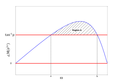
Figure 6: Illustration of Theorem IV.3. The result is given in terms of $\rho$ while the phase of the multiplier $M$ is $\tan^{-1}\rho$.

.

An algorithm for finding the phase limitation in Theorem IV.3 part (i) for a second order plant is given in [54]. For a given stable plant $G$ and a value of $k$ such that $0<k<k_{N}$ the phase of an ideal multiplier is obtained as

$$\angle M_{d}=\begin{cases}\angle(G+1/k)-90&\text{if}\quad\angle(G+1/k)>90\\ \angle(G+1/k)+90&\text{if}\quad\angle(G+1/k)<-90\\ 0&\text{otherwise}.\\ \end{cases}$$ (53)

Then the algorithm increases $k$ until the existence of such a multiplier can be discarded by using the limitation presented in Theorem IV.3.

IV-B Integral bound and sparsely parametrized multipliers

Theorem IV.3 gives relative bounds on the real and imaginary parts of a Zames-Falb multiplier’s frequency response over an interval $[a,b]$. It is straightforward to derive a closely related result in terms of the integrals over the same interval.

Theorem IV.5.

Let $M$ be a discrete-time Zames-Falb multiplier. Suppose

$$\int_{a}^{b}\mbox{Im}(M(e^{j\omega}))\,d\omega >\rho\int_{a}^{b}\mbox{Re}(M(e^{j\omega}))\,d\omega$$ (54)

for some $\rho>0$. Then

1. $\rho<\rho^{d}$ if $M\in\mathcal{M}^{d}$,

2. $\rho<\rho^{d}_{odd}$ if $M\in\mathcal{M}^{d}_{odd}$.

Proof:

See Appendix.

Remark IV.6.

Theorem IV.5 is stronger than Theorem IV.3 in the sense that condition (51) is sufficient for condition (54) but not necessary. Theorem IV.3 may be derived as a Corollary of Theorem IV.5 by applying the Mean Value Theorem [58].

Theorem IV.5 gives a tight phase limitation in the sense that we can associate a set of sparsely parameterized multipliers with Theorem IV.5 as follows.

Proposition IV.7.

1. For a given $a$ and $b$, define the set $\mathcal{N}^{d}\subset\mathbb{Z}$ as the set of integers $n$ such that $\psi_{d}(n)/\phi_{d}(n)=\rho^{d}$. Then multipliers of the form

   $$M(z)=1-\sum_{n\in\mathcal{N}^{d}}h_{n}z^{-n}$$ (55)

   with

   $$h_{0}=0\mbox{, }h_{n}\geq 0\mbox{ and }\sum_{n\in\mathcal{N}([a,b])}h_{n}=1-\varepsilon$$ (56)

   satisfy (54) with $\rho$ arbitrarily close to $\rho^{d}$ in the limit as $\varepsilon\rightarrow 0$.

2. For a given $a$ and $b$, define the set $\mathcal{N}^{d}_{odd}\subset\mathbb{Z}$ as the set of integers $n$ such that $\psi_{d}(n)/\tilde{\phi}_{d}(n)=\rho^{d}_{odd}$. Then multipliers of the form

   $$M(z)=1-\sum_{n\in\mathcal{N}^{d}}h_{n}z^{-n}$$ (57)

   with

   $$h_{0}=0\mbox{ and }\sum_{n\in\mathcal{N}([a,b])}h_{n}=1-\varepsilon$$ (58)

   satisfy (54) with $\rho$ arbitrarily close to $\rho^{d}_{odd}$ in the limit as $\varepsilon\rightarrow 0$.

Proof:

See Appendix.

Remark IV.8.

It is, once again, straightforward to produce the counterpart of Theorem IV.5 with (54) replaced by

$$\int_{a}^{b}\mbox{Im}(M(e^{j\omega}))\,d\omega<-\rho\int_{a}^{b}\mbox{Re}(M(e^{j\omega}))\,d\omega.$$ (59)

Similarly for Theorem IV.7 with (i) $\psi_{d}(n)/\phi_{d}(n)=-\rho^{d}$ and (ii) $\psi_{d}(n)/\tilde{\phi}_{d}(n)=-\rho^{d}_{odd}$.

As an illustrative example, suppose $a=0.7$ and $b=0.77501$ (approx.). Then

$$\tan^{-1}\rho^{d}\approx 76.8^{\circ},$$ (60)

and

$$\mathcal{N}^{d}=\left\{-8,9\right\}.$$ (61)

Fig 7 shows the phases of the limiting cases $M(z)=1-z^{8}$, $M(z)=1-z^{-9}$ and linear combinations of the form $M(z)=1-\lambda z^{8}-(1-\lambda)z^{-9}$ with $0<\lambda<1$. It can be seen that the phases are near to $\tan^{-1}\rho^{d}$ over the interval $[a,b]$. However they always have values both above and below, indicating that Theorem IV.3 is not tight in the same sense as Theorem IV.5.

Remark IV.9.

A similar analysis is possible for continuous-time multipliers. Compare Remark III.7.

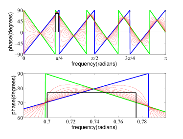
Figure 7: Phases of the limiting cases $M(z)=1-z^{8}$, $M(z)=1-z^{-9}$ and linear combinations of the form $M(z)=1-\lambda z^{8}-(1-\lambda)z^{-9}$ with $0<\lambda<1$. The phase limitation $\tan^{-1}\rho^{d}\approx 76.8^{\circ}$ over the interval $[a,b]=[0.7,0.77501]$ is also shown. The top figure shows the phase over the frequency range from $0$ to $\pi$ radians, while the bottom figure shows the same data in the frequency range from $0.68$ to $0.8$ radians.

IV-C Discrete-time counterparts of the off-axis circle criterion

The off-axis circle criterion [3] (Theorem II.10) is a useful frequency-based graphical stability test for continuous-time systems. It is sometimes assumed (e.g. in [52]) that its discrete-time counterpart is true. We state this as a conjecture:

Conjecture IV.10.

Consider the feedback system in Fig. 2 with $G\in\mathbf{RH}_{\infty}$, and $\phi$ is slope-restricted in $S[0,k]$. Suppose that the Nyquist plot of the linear part of the system $G(e^{j\omega})$ lies entirely to the right of a straight line passing through the point $(-\frac{1}{k}+\delta,0)$ where $\delta>0$ and $\phi$ is monotonically increasing. Then the feedback interconnection (2) is $\ell_{2}$-stable.

A geometrical interpretation of both Theorem II.10 for continuous-time systems and Conjecture IV.10 for discrete-time systems is given in Fig 8.

The phase-limitation on discrete-time Zames-Falb multipliers carries the implication that there can be no multiplier construction corresponding to that for RL/RC multipliers of [42] used to prove Theorem II.10. We summarise the argument as follows:

Figure 8: Geometrical interpretation of the off-axis circle criterion considering the plant $G$ (Theorem II.10 for continuous-time systems and Conjecture IV.10 for discrete-time systems). The Theorem for continuous-time systems is true but the Conjecture for discrete-time systems is false in general.

1. Under the conditions of Conjecture IV.10 there is some $\theta$ in $(-90,90)$ degrees such that the phase of $1+kG$ always lies in the interval $(-90-\theta,90-\theta)$ degrees. Hence an ideal LTI multiplier with constant phase $\theta$ would render the real part of $M(1+kG)$ positive over all frequencies.

2. In their proof of the continuous off-axis circle criterion Cho and Narendra [3] show that it is possible to construct RL/RC multipliers whose phase is arbitrarily close to some constant $\theta$ degrees over an arbitrarily large interval. We show that for some values of $\theta$ this may not be possible for any discrete-time LTI multiplier.

3. If a discrete-time LTI multiplier preserves the positivity of a slope-restricted nonlinearity then there is a Zames-Falb multiplier with the same phase [14], [43], so we can limit our set of multipliers to the class of LTI Zames-Falb multipliers.

4. If $\theta>\tan^{-1}(2/\pi)\approx 32.48^{\circ}$ then Theorem IV.3 precludes any such construction of a Zames-Falb multiplier since if $a\rightarrow 0^{+}$ and $b\rightarrow\pi^{-}$ then $\rho^{d}\rightarrow\tan^{-1}(-2/\pi)$.

Hence the phase limitation can be used to invalidate Conjecture IV.10 when $\theta>\tan^{-1}(2/\pi)$. Smaller values can be obtained by using different values of $a$ and $b$. It follows that any counterpart of the off-axis circle criterion in discrete-time must take into account specific information about frequency intervals. This is true of the more limited result originally derived by Narendra and Cho [42] (Theorem II.11). In fact it can be shown that the counterexamples to the Kalman conjecture of [50] and [51] are also counterexamples to Conjecture IV.10.

IV-D Finite search in discrete-time domain

Here we provide a result which simplifies the numerical implementation. Although the definitions of $\rho^{d}$ and $\rho^{d}_{odd}$ are given with an infinite number of terms, they can be calculated using a finite number $n=n_{N}$ given in Lemma IV.11.

Lemma IV.11.

Let $0\leq a<b\leq\pi$, then

$$\rho^{d}=\max_{1\leq n\leq n_{N}}\frac{|\psi_{d}(n)|}{\phi_{d}(n)},$$ (62)

and

$$\rho^{d}_{odd}=\max_{1\leq n\leq n_{N}}\frac{|\psi_{d}(n)|}{\tilde{\phi}_{d}(n)},$$ (63)

with

$$n_{N}=\lfloor\nu\rfloor,$$ (64)

where

$$\nu=\frac{2(b-a)-2\sin b+2\sin a-2\cos b+2\cos a}{(a-b)(\cos b-\cos a)}.$$ (65)

Proof:

See Appendix.

Suppose we wish to find a phase limitation over the interval $\omega\in[0.7,0.75]$. Applying Lemma IV.11 we find $\nu=55.2$ and hence $|\psi_{d}(n)|/\phi_{d}(n)<|\psi_{d}(1)|/\phi_{d}(1)$ for all $n>n_{N}$, with

$$n_{N}=55.$$ (66)

Hence it is sufficient to search over the integers $1\leq n\leq 55$ for $\rho^{d}$. The numerical results shown in Fig. 9 demonstrate that $|\psi_{d}(n)|/\phi_{d}(n)<|\psi_{d}(1)|/\phi_{d}(1)$ for all $n>18$. In fact the maximum occurs at $n=-9$.

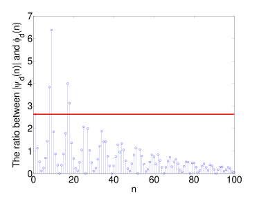
Figure 9: The value of $f_{d}(n)$ with different value of $n$

IV-E Numerical example

Let us consider the negative feedback interconnection between the plant

$$G(z)=\frac{z}{z^{2}-1.8z+0.81},$$ (67)

and a slope-restricted nonlinearity. This second-order plant is a counterexample to the discrete-time Kalman conjecture as there is a periodic solution when $k=2.1$ [50], and the Nyquist value is $k_{N}=3.61$. Using the algorithm of [24] we find there exists a Zames-Falb multiplier for non-odd nonlinearities when $\hat{k}_{ZF}=1.3028$.

Using the phase limitation result given in Theorem IV.3 part (i), it is possible to show that there is no Zames-Falb multiplier for any $k>k_{PL}=1.4603$. Fig. 10 illustrates that the phase limitation results indicate there can be no appropriate Zames-Falb multiplier when $k=1.5$. The phase limitation is given by $\tan^{-1}\rho^{d}=66.7137^{\circ}$, where $\rho^{d}$ is obtained using Definition IV.1 with $a=0.7198$ and $b=0.8996$. By contrast, Fig. 11 shows that this limitation is not active when $k=\hat{k}_{ZF}$; this is expected since we have been able to find a suitable Zames-Falb multiplier for this value of the gain. A complete list of slope restriction results of $G(z)$ in (67) is given in Table II. The result of the reduced off-axis circle criterion $k_{R}$ shows conservativeness compared to all the other results in the Table. The (false) result from the direct discrete-time counterpart of the off-axis circle criterion is greater than the slope obtained by phase limitation, i.e. $k_{O}>k_{PL}$; this demonstrates that Conjecture IV.10 is false.

Finally, using combination of deadzone and saturation as nonlinearity, we are able to find periodic solution with $\hat{k}_{C}=1.3666$. These results are consistent with Conjecture I.2, i.e. $\hat{k}_{ZF}<\hat{k}_{C}<k_{PL}$.

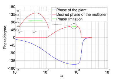
Figure 10: Phase of $(1+1.5G)$, desired phase of the multiplier and the phase limitation

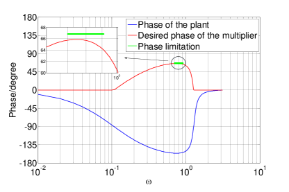
Figure 11: Phase of $(1+1.3028G)$, desired phase of the multiplier and the phase limitation

TABLE II: Results of different slope restrictions (non-odd nonlinearity)

$k$	$k_{RO}$	$\hat{k}_{ZF}$	$\hat{k}_{C}$	$k_{PL}$	$k_{O}$	$k_{N}$
Result	0.8962	1.3028	1.3666	1.4603	3.61	3.61

V Conclusions

In this paper we have demonstrated the connection between phase limitations of Zames-Falb multipliers and the Kalman conjecture.

In continuous time, we have generalised a limitation proposed by Megretski, clarified its remit and illustrated its effect with a numerical example. In particular we show it can be applied to a fourth-order plant where the resulting numerical implementation shows instability. It remains open which choice of intervals $[a,b]$ and $[c,d]$ and scaling parameter $\kappa$ in Theorem III.4 provides most insight.

Motivated by this connection and recent results on the Kalman conjecture in discrete time, we have derived a more simple phase limitation for discrete-time Zames-Falb multipliers. Numerical results in discrete time are easier to obtain and we show that the slope restriction obtained by using phase limitation theorems can be about 40% of the Nyquist value even for some second-order examples. Thus the phase limitation can be directly useful when forming benchmarks for searches over Zames-Falb multipliers. Further, the phase limitation can be used to show there can be no direct counterpart in discrete time (Conjecture IV.10) to the off-axis circle criterion for continuous-time systems (Theorem II.10).

Based on the results of this paper, we propose Conjecture I.2, which seems to be compatible with current state-of-the-art knowledge and results for both continuous and discrete-time domains.

There is plenty of scope for future work. It seems possible that the phase limitations might be used to provide a more computationally efficient search fo appropriate multipliers. Phase limitations for the class of Zames-Falb multipliers available when the nonlinearity is quasi-odd [36] require further research.

VI Acknowledgements

We would like to thank the anonymous reviewers for their helpful suggestions.

VII Appendix

VII-A Proof of Lemma III.2

Both the functions

$$f_{1}(\omega)=\omega-\frac{\sin\omega t}{t}$$ (68)

and

$$f_{2}(\omega)=\omega+\frac{\sin\omega t}{t}$$ (69)

are monotone non-decreasing in $\omega$ when $t>0$. It follows that $\phi(t)>0$ and $\tilde{\phi}(t)>0$ when $t>0$. In addition

$$\lim_{t\rightarrow\infty}\phi(t)=\lambda(b-a)+\kappa\mu(d-c)>0,$$ (70)

and

$$\lim_{t\rightarrow\infty}\tilde{\phi}(t)=\lambda(b-a)+\kappa\mu(d-c)>0.$$ (71)

Finally

$$\phi_{1}(t)=-[\lambda(b-a)+\kappa\mu(d-c)]\\ +\lambda\frac{(b^{3}-a^{3})t^{2}}{6}+\kappa\mu\frac{(d^{3}-c^{3})t^{2}}{6}+O(t^{4})\mbox{ as }t\rightarrow 0,$$ (72)

and

$$\psi(t)=\lambda\frac{(b^{2}-a^{2})t}{2}-\mu\frac{(d^{2}-c^{2})t}{2}\\ -\lambda\frac{(b^{4}-a^{4})t^{3}}{24}+\mu\frac{(d^{4}-c^{4})t^{3}}{24}+O(t^{5})\mbox{ as }t\rightarrow 0,$$ (73)

so the choice (28) ensures

$$\lim_{t\rightarrow 0}\frac{|\psi(t)|}{\phi(t)}=0,$$ (74)

and

$$\lim_{t\rightarrow 0}\frac{|\psi(t)|}{\tilde{\phi}(t)}=0.$$ (75)

VII-B Proof of Theorem III.4

Suppose (31) and (32) hold for some multiplier $M(j\omega)=1-H(j\omega)$. Then

$$\mbox{Im}(M(j\omega))=\int_{-\infty}^{\infty}\sin(\omega t)h(t)\,dt,$$ (76)

and

$$\mbox{Re}(M(j\omega))=1-\int_{-\infty}^{\infty}\cos(\omega t)h(t)\,dt,$$ (77)

where $h$ in the impulse response of $H$. Hence integrating (31) and (32) over their respective intervals gives

$$\int_{-\infty}^{\infty}\frac{\cos(at)-\cos(bt)}{t}h(t)\,dt>\\ \rho(b-a)+\rho\int_{-\infty}^{\infty}\frac{\sin(at)-\sin(bt)}{t}h(t)\,dt,$$ (78)

and

$$\int_{-\infty}^{\infty}\frac{\cos(ct)-\cos(dt)}{t}h(t)\,dt<\\ -\kappa\rho(d-c)-\kappa\rho\int_{-\infty}^{\infty}\frac{\sin(ct)-\sin(dt)}{t}h(t)\,dt.$$ (79)

Summing the two inequalities, multiplied by $\lambda$ and $-\mu$ respectively, gives

$$\int_{-\infty}^{\infty}\psi(t)h(t)dt>\\ \rho[\lambda(b-a)+\kappa\mu(d-c)]+\rho\int_{-\infty}^{\infty}\phi_{1}h(t)\,dt.$$ (80)

1. If $M\in\mathcal{M}^{c}$ then $\|h\|_{1}<1$ and $h(t)\geq 0$ for all $t$. So

   $$\rho[\lambda(b-a)+\kappa\mu(d-c)]>\\ \int_{-\infty}^{\infty}\rho[\lambda(b-a)+\kappa\mu(d-c)]h(t)\,dt.$$ (81)

   and hence we can write (80) as

   $$\int_{-\infty}^{\infty}(\psi(t)-\rho\phi(t))h(t)\,dt>0.$$ (82)

   But, since $\phi$ is an even function and $\psi$ is an odd function,

   $$\psi(t)-\rho^{c}\phi(t)\leq 0\mbox{ for all }t.$$ (83)

   Further, since $\phi$ is non-negative,

   $$\psi(t)-\rho\phi(t)\leq 0\mbox{ for all }t\mbox{ when }\rho\geq\rho^{c}.$$ (84)

   Hence $\rho<\rho^{c}$.

2. If $M\in\mathcal{M}^{c}_{odd}$ then we can only say $\|h\|_{1}<1$. Nevertheless,

   $$\rho[\lambda(b-a)+\kappa\mu(d-c)]>\\ \int_{-\infty}^{\infty}\rho[\lambda(b-a)+\kappa\mu(d-c)]|h(t)|\,dt.$$ (85)

   and hence (80) leads to

   $$\int_{-\infty}^{\infty}(|\psi(t)|-\rho\tilde{\phi}(t))|h(t)|\,dt>0.$$ (86)

   But, since $\tilde{\phi}$ is also an even function and (as before) $\psi$ is an odd function,

   $$|\psi(t)|-\rho^{c}_{odd}\tilde{\phi}(t)\leq 0\mbox{ for all }t.$$ (87)

   Further, since $\tilde{\phi}$ is non-negative,

   $$|\psi(t)|-\rho\tilde{\phi}(t)\leq 0\mbox{ for all }t\mbox{ when }\rho\geq\rho^{c}_{odd}.$$ (88)

   Hence $\rho<\rho^{c}_{odd}$.

VII-C Proof of Lemma IV.2

The result is immediate following a similar argument to the proof of Lemma III.2. In particular, as $\phi_{d}$ and $\tilde{\phi}_{d}$ are evaluated for discrete values of $n\geq 1$, their limiting behaviour as $n\rightarrow 0$ need not be considered.

VII-D Proof of Theorem IV.3

Suppose (51) holds for some multiplier $M(e^{j\omega})=1-H(e^{j\omega})$. Then

$$\mbox{Im}(M(e^{j\omega}))=\sum_{n=-\infty}^{\infty}\sin(\omega n)h_{n}$$ (89)

and

$$\mbox{Re}(M(e^{j\omega}))=1-\sum_{n=-\infty}^{\infty}\cos(\omega n)h_{n},$$ (90)

where $h$ is the impulse response of $H$. Hence integrating (51) over the interval $[a,b]$ gives

$$\sum_{n=-\infty}^{\infty}\frac{\cos(an)-\cos(bn)}{n}h_{n}>\\ \rho(b-a)+\rho\sum_{n=-\infty}^{\infty}\frac{\sin(an)-\sin(bn)}{n}h_{n}.$$ (91)

1. If $M\in\mathcal{M}^{d}$ then $h_{0}=0$, $\|h\|_{1}<1$ and $h_{n}\geq 0$ for all $n$. So

   $$\rho(b-a)>\sum_{n=-\infty}^{\infty}\rho(b-a)h_{n},$$ (92)

   and hence we can write (91) as

   $$\sum_{n=-\infty}^{\infty}(\psi_{d}(n)-\rho\phi_{d}(n))h_{n}>0.$$ (93)

   But, since $\phi_{d}$ is an even function and $\psi_{d}$ is an odd function,

   $$\psi_{d}(n)-\rho^{d}\phi_{d}(n)\leq 0\mbox{ for all }n\geq 1.$$ (94)

   Further, since $\phi_{d}$ is non-negative,

   $$\psi_{d}(n)-\rho\phi_{d}(n)\leq 0\mbox{ for all }n\geq 1\mbox{ when }\rho\geq\rho^{d}.$$ (95)

   Hence $\rho<\rho^{d}$.

2. If $M\in\mathcal{M}^{d}_{odd}$ then we can only say $h_{0}=0$ and $\|h\|_{1}<1$. Nevertheless,

   $$\rho(b-a)>\sum_{n=-\infty}^{\infty}\rho(b-a)|h_{n}|,$$ (96)

   and hence (91) leads to

   $$\sum_{n=-\infty}^{\infty}(|\psi_{d}(n)|-\rho\tilde{\phi}_{d}(n))|h_{n}|>0.$$ (97)

   But, since $\tilde{\phi}_{d}$ is also an even function and (as before) $\psi_{d}$ is an odd function,

   $$|\psi_{d}(n)|-\rho^{d}_{odd}\tilde{\phi}_{d}(n)\leq 0\mbox{ for all }n\geq 1.$$ (98)

   Further, since $\tilde{\phi}_{d}$ is non-negative,

   $$|\psi_{d}(n)|-\rho\tilde{\phi}_{d}(n)\leq 0\mbox{ for all }n\geq 1\mbox{ when }\rho\geq\rho^{d}_{odd}.$$ (99)

   Hence $\rho<\rho^{d}_{odd}$.

VII-E Proof of Theorem IV.5

Substituting

$$\mbox{Im}(M(e^{j\omega}))=\sum_{n=-\infty}^{\infty}\sin(\omega n)h_{n}$$ (100)

and

$$\mbox{Re}(M(e^{j\omega}))=1-\sum_{n=-\infty}^{\infty}\cos(\omega n)h_{n},$$ (101)

into (54) leads to (91). The proof is then identical to that of Theorem IV.3.

VII-F Proof of Proposition IV.7

1. Let $M_{n}(z)=1-z^{-n}$ with $n\in\mathcal{N}([a,b])$. Then

   $$\mbox{Im}(M_{n}(e^{j\omega})) =\sin(\omega n),$$ (102)

   $$\mbox{Re}(M_{n}(e^{j\omega})) =1-\cos(\omega n).$$ (103)

   Integrating over the interval yields

   $$\int_{a}^{b}\mbox{Im}(M(e^{j\omega}))\,d\omega=\rho^{c}\int_{a}^{b}\mbox{Re}(M(e^{j\omega}))\,d\omega.$$ (104)

   Furthermore, if

   $$M(z)=1-\sum_{n\in\mathcal{N}([a,b])}\lambda_{n}z^{-n},$$ (105)

   with

   $$\lambda_{n}\geq 0\mbox{ and }\sum_{n\in\mathcal{N}([a,b])}\lambda_{n}=1,$$ (106)

   then we may write

   $$M(z)=\sum_{n\in\mathcal{N}([a,b])}M_{n}(z).$$ (107)

   The proof follows straightforwardly.

2. Similar.

VII-G Proof of Lemma IV.11

Let

$$\epsilon =\frac{|\psi_{d}(1)|}{\phi_{d}(1)}=\frac{|\cos{a}-\cos{b}|}{b-a-(\sin{b}-\sin{a})}$$ (108)

$$=-\frac{\cos{b}-\cos{a}}{b-a-(\sin{b}-\sin{a})}=-\frac{\psi_{d}(1)}{\phi_{d}(1)},$$

where we have used that $(x-\sin x)$ is a monotonically increasing function; and

$$\nu =\frac{2}{(b-a)}\frac{1+\epsilon}{\epsilon}=\frac{2-2\psi_{d}(1)/\phi_{d}(1)}{-(b-a)\psi_{d}(1)/\phi_{d}(1)}$$ (109)

$$=\frac{2(b-a)-2\sin b+2\sin a-2\cos b+2\cos a}{(a-b)(\cos b-\cos a)}.$$

For $n>\nu$, we know $(b-a)n-2>0$. In addition,

$$\epsilon(b-a)n>2+2\epsilon,$$ (110)

so

$$\frac{|\psi_{d}(n)|}{\phi_{d}(n)}=\frac{|\cos{(bn)}-\cos{(an)}|}{(b-a)n-[\sin{(bn)}-\sin{(an)}]}<\frac{2}{(b-a)n-2}<\epsilon.$$ (111)

As a result,

$$\frac{|\psi_{d}(n)|}{\phi_{d}(n)}<\frac{|\psi_{d}(1)|}{\phi_{d}(1)}\qquad\forall n>\nu.$$ (112)

Finally, it is easy to check that

$$\frac{|\psi_{d}(1)|}{\tilde{\phi}_{d}(1)}=\frac{|\psi_{d}(1)|}{\phi_{d}(1)}$$ (113)

and hence the same relation holds for $|\psi_{d}(n)|/\tilde{\phi}_{d}(n)$.

Shuai Wang is a PhD candidate at the School of Electrical and Electronic Engineering, University of Manchester, UK. He received a Bachelor degree in Measurement and Control, Technology & Instrument, and a Master degree in Instrument Science & Technology from Harbin Institute of Technology, Harbin, China in 2011 and 2013 respectively. His research interests include absolute stability and multiplier theory. He is a member of IEEE, IET and SIAM.

Joaquin Carrasco is a Lecturer at the Control Systems Centre, School of Electrical and Electronic Engineering, University of Manchester, UK. He was born in Abarán, Spain, in 1978. He received the B.Sc. degree in physics and the Ph.D. degree in control engineering from the University of Murcia, Murcia, Spain, in 2004 and 2009, respectively. From 2009 to 2010, he was with the Institute of Measurement and Automatic Control, Leibniz Universität Hannover, Hannover, Germany. From 2010 to 2011, he was a research associate at the Control Systems Centre, School of Electrical and Electronic Engineering, University of Manchester, UK. He has been a Visiting Researcher at the University of Groningen, Groningen, The Netherlands, and the University of Massachusetts, Amherst. His current research interests include absolute stability, multiplier theory, and robotics applications. He is a member of the IFAC technical committee Telematics: Control via Communication Networks.

William P. Heath is Chair of Feedback and Control at the School of Electrical and Electronic Engineering, University of Manchester, UK. He received a B.A. in Mathematics from Cambridge University in 1987, and both an M.Sc. and a Ph.D. from UMIST in 1989 and 1992 respectively. He was with Lucas Automotive from 1995 to 1998 and was a Research Academic at the University of Newcastle, Australia from 1998 to 2004. His interests include absolute stability, multiplier theory, constrained control and system identification.

References

- [1] M. Vidyasagar, Nonlinear systems analysis. Prentice Hall, 1978.
- [2] H. K. Khalil, “Nonlinear systems, 3rd ed.” Prentice Hall Upper Saddle River, 2002.
- [3] Y.-S. Cho and K. Narendra, “An off-axis circle criterion for stability of feedback systems with a monotonic nonlinearity,” IEEE Transactions on Automatic Control, vol. 13, no. 4, pp. 413–416, 1968.
- [4] C. J. Harris and J. Valenca, The stability of input-output dynamical systems. Elsevier, 1983.
- [5] Y. Z. Tsypkin, “On the stability in the large of nonlinear sampled-data systems,” Doklady Akademii Nauk SSSR, vol. 145, pp. 52–55, 1962.
- [6] ——, “A criterion for absolute stability of automatic pulse systems with monotonic characteristics of the nonlinear element,” in Soviet Physics Doklady, vol. 9, 1964, p. 263.
- [7] E. Jury and B. Lee, “On the stability of a certain class of nonlinear sampled-data systems,” IEEE Transactions on Automatic Control, vol. 9, no. 1, pp. 51–61, 1964.
- [8] ——, “On the absolute stability of nonlinear sampled-data systems,” IEEE Transactions on Automatic Control, vol. 9, no. 1, pp. 551–554, 1964.
- [9] N. S. Ahmad, W. P. Heath, and G. Li, “LMI-based stability criteria for discrete-time Lur’e systems with monotonic, sector-and slope-restricted nonlinearities,” IEEE Transactions on Automatic Control, vol. 58, no. 2, pp. 459–465, 2013.
- [10] N. S. Ahmad, J. Carrasco, and W. P. Heath, “A less conservative LMI condition for stability of discrete-time systems with slope-restricted nonlinearities,” IEEE Transactions on Automatic Control, vol. 60, no. 6, pp. 1692–1697, 2015.
- [11] R. O’Shea, “An improved frequency time domain stability criterion for autonomous continuous systems,” IEEE Transactions on Automatic Control, vol. 12, no. 6, pp. 725–731, 1967.
- [12] G. Zames and P. L. Falb, “Stability conditions for systems with monotone and slope-restricted nonlinearities,” SIAM Journal on Control, vol. 6, no. 1, pp. 89–108, 1968.
- [13] R. O’Shea and M. Younis, “A frequency-time domain stability criterion for sampled-data systems,” IEEE Transactions on Automatic Control, vol. 12, no. 6, pp. 719–724, 1967.
- [14] J. Willems and R. Brockett, “Some new rearrangement inequalities having application in stability analysis,” IEEE Transactions on Automatic Control, vol. 13, no. 5, pp. 539–549, 1968.
- [15] C. Desoer and M. Vidyasagar, Feedback Systems: Input–Output Properties. Academic Press, Orlando, FL, USA, 1975.
- [16] M. Safonov and G. Wyetzner, “Computer-aided stability analysis renders Popov criterion obsolete,” IEEE Transactions on Automatic Control, vol. 32, no. 12, pp. 1128–1131, 1987.
- [17] X. Chen and J. T. Wen, “Robustness analysis of LTI systems with structured incrementally sector bounded nonlinearities,” in Proceedings of the American Control Conference, vol. 5, 1995, pp. 3883–3887.
- [18] ——, “Robustness analysis for linear time-invariant systems with structured incrementally sector bounded feedback nonlinearities,” Applied Mathematics and Computer Science, vol. 6, pp. 623–648, 1996.
- [19] M. C. Turner, M. Kerr, and I. Postlethwaite, “On the existence of stable, causal multipliers for systems with slope-restricted nonlinearities,” IEEE Transactions on Automatic Control, vol. 54, no. 11, pp. 2697–2702, 2009.
- [20] M. Chang, R. Mancera, and M. Safonov, “Computation of Zames-Falb multipliers revisited,” IEEE Transactions on Automatic Control, vol. 57, no. 4, p. 1024, 2012.
- [21] J. Carrasco, W. P. Heath, G. Li, and A. Lanzon, “Comments on “On the existence of stable, causal multipliers for systems with slope-restricted nonlinearities”,” IEEE Transactions on Automatic Control, vol. 57, no. 9, pp. 2422–2428, 2012.
- [22] J. Carrasco, M. Maya-Gonzalez, A. Lanzon, and W. P. Heath, “LMI searches for anticausal and noncausal rational Zames–Falb multipliers,” Systems & Control Letters, vol. 70, pp. 17–22, 2014.
- [23] N. S. Ahmad, J. Carrasco, and W. P. Heath, “LMI searches for discrete-time Zames-Falb multipliers,” in 52nd IEEE Conference on Decision and Control, 2013, pp. 5258–5263.
- [24] S. Wang, W. P. Heath, and J. Carrasco, “A complete and convex search for discrete-time noncausal FIR Zames-Falb multipliers,” in Proceedings of the 53rd IEEE Conference on Decision and Control, 2014, pp. 3918–3923.
- [25] A. Megretski and A. Rantzer, “System analysis via Integral Quadratic Constraints,” IEEE Transactions on Automatic Control, vol. 42, no. 6, pp. 819–830, 1997.
- [26] C.-Y. Kao, A. Megretski, U. Jönsson, and A. Rantzer, “A MATLAB toolbox for robustness analysis,” in IEEE International Symposium on Computer Aided Control Systems Design, 2004, pp. 297–302.
- [27] J. Veenman, C. W. Scherer, and H. Köroğlu, “Robust stability and performance analysis based on integral quadratic constraints,” European Journal of Control, vol. 31, pp. 1–32, 2016.
- [28] D. Altshuller, Frequency Domain Criteria for Absolute Stability: A Delay-integral-quadratic Constraints Approach. Springer, 2013.
- [29] M. G. Safonov and V. V. Kulkarni, “Zames-falb multipliers for MIMO nonlinearities,” in Proceedings of the American Control Conference, vol. 6. IEEE, 2000, pp. 4144–4148.
- [30] F. J. D’Amato, M. A. Rotea, A. V. Megretski, and U. T. Jönsson, “New results for analysis of systems with repeated nonlinearities,” Automatica, vol. 37, no. 5, pp. 739–747, 2001.
- [31] R. Mancera and M. G. Safonov, “All stability multipliers for repeated MIMO nonlinearities,” Systems & Control Letters, vol. 54, no. 4, pp. 389–397, 2005.
- [32] M. C. Turner, M. L. Kerr, and I. Postlethwaite, “On the existence of multipliers for MIMO systems with repeated slope-restricted nonlinearities,” in ICCAS-SICE, 2009, pp. 1052–1057.
- [33] M. Fetzer and C. W. Scherer, “Full-block multipliers for repeated, slope-restricted scalar nonlinearities,” International Journal of Robust and Nonlinear Control, 2017, DOI: 10.1002/rnc.3751.
- [34] A. Rantzer, “Friction analysis based on integral quadratic constraints,” Int. J. Robust Nonlinear Control, vol. 11, no. 7, pp. 645––652, 2001.
- [35] D. Materassi and M. V. Salapaka, “A generalized Zames-Falb multiplier,” IEEE Transactions on Automatic Control, vol. 56, no. 6, pp. 1432–1436, 2011.
- [36] W. P. Heath, J. Carrasco, and D. A. Altshuller, “Stability analysis of asymmetric saturation via generalised Zames-Falb multipliers,” in Proceedings of the 54th IEEE Conference on Decision and Control, 2015, pp. 3748–3753.
- [37] M. C. Turner and M. L. Kerr, “ gain bounds for systems with sector bounded and slope-restricted nonlinearities,” International Journal of Robust and Nonlinear Control, vol. 22, no. 13, pp. 1505–1521, 2012.
- [38] B. Hu, M. J. Lacerda, and P. Seiler, “Robustness analysis of uncertain discrete-time systems with dissipation inequalities and integral quadratic constraints,” International Journal of Robust and Nonlinear Control, 2016, DOI: 10.1002/rnc.3646.
- [39] J. Carrasco, W. P. Heath, and A. Lanzon, “Equivalence between classes of multipliers for slope-restricted nonlinearities,” Automatica, vol. 49, no. 6, pp. 1732–1740, 2013.
- [40] W. P. Heath and A. G. Wills, “Zames-Falb multipliers for quadratic programming,” in Proceedings of the 44th IEEE Annual Conference on Decision and Control (CDC). IEEE, 2005, pp. 963–968.
- [41] L. Lessard, B. Recht, and A. Packard, “Analysis and design of optimization algorithms via integral quadratic constraints,” SIAM Journal on Optimization, vol. 26, no. 1, pp. 57–95, 2016.
- [42] K. S. Narendra and Y.-S. Cho, “Stability analysis of nonlinear and time-varying discrete systems,” SIAM Journal on Control, vol. 6, no. 4, pp. 625–646, 1968.
- [43] J. C. Willems, The analysis of feedback systems. The MIT Press, 1971.
- [44] J. Carrasco, W. P. Heath, and A. Lanzon, “On multipliers for bounded and monotone nonlinearities,” Systems & Control Letters, vol. 66, pp. 65–71, 2014.
- [45] J. Carrasco, M. C. Turner, and W. P. Heath, “Zames–Falb multipliers for absolute stability: From O’Shea’s contribution to convex searches,” European Journal of Control, vol. 28, pp. 1–19, 2016.
- [46] A. Megretski, “Combining L1 and L2 methods in the robust stability and performance analysis of nonlinear systems,” in Proceedings of the 34th IEEE Conference on Decision and Control, vol. 3, 1995, pp. 3176–3181.
- [47] U. Jönsson and M.-C. Laiou, “Stability analysis of systems with nonlinearities,” in Proceedings of the 35th IEEE Conference on Decision and Control, vol. 2, 1996, pp. 2145–2150.
- [48] U. Jönsson, “Robustness analysis of uncertain and nonlinear systems,” Department of Automatic Control, Lund Institute of Technology, vol. 1047, 1996.
- [49] N. Barabanov, “On the Kalman problem,” Siberian Mathematical Journal, vol. 29, no. 3, pp. 333–341, 1988.
- [50] J. Carrasco, W. P. Heath, and M. de la Sen, “Second order counterexample to the Kalman conjecture in discrete-time,” in Proceeding of the European Control Conference, 2015.
- [51] W. P. Heath, J. Carrasco, and M. de la Sen, “Second-order counterexamples to the discrete-time Kalman conjecture,” Automatica, vol. 60, pp. 140–144, 2015.
- [52] A. R. Plummer and C. Ling, “Stability and robustness for discrete-time systems with control signal saturation,” Proceedings of the Institution of Mechanical Engineers, Part I: Journal of Systems and Control Engineering, vol. 214, no. 1, pp. 65–76, 2000.
- [53] Y. Okuyama, T. Kosaka, and F. Takemori, “Robust stability analysis for nonlinear sampled-data control systems in a frequency domain,” in Proceedings of the European Control Conference (ECC),, 1999, pp. 2668–2673.
- [54] S. Wang, J. Carrasco, and W. P. Heath, “Phase limitations of discrete-time Zames-Falb multipliers,” in Proceedings of the 54th IEEE Conference on Decision and Control, 2015, pp. 5707–5712.
- [55] R. E. Kalman, “Physical and mathematical mechanisms of instability in nonlinear automatic control systems,” Trans. ASME, vol. 79, no. 3, pp. 553–566, 1957.
- [56] R. Fitts, “Two counterexamples to Aizerman’s conjecture,” IEEE Transactions on Automatic Control, vol. 11, no. 3, pp. 553–556, 1966.
- [57] G. A. Leonov and N. V. Kuznetsov, “Hidden attractors in dynamical systems. From hidden oscillations in Hilbert–Kolmogorov, Aizerman, and Kalman problems to hidden chaotic attractor in Chua circuits,” International Journal of Bifurcation and Chaos, vol. 23, no. 01, p. 1330002, 2013.
- [58] T. M. Apostol, Mathematical analysis, 2nd ed. Addison Wesley, 1974.
- [59] J. Bechhoefer, “Kramers-Kronig, Bode, and the meaning of zero,” American Journal of Physics, vol. 79, no. 10, pp. 1053–1059, 2011.
- [60] Y. Li and Z. Lin, “On the estimation of the domain of attraction for linear systems with asymmetric actuator saturation via asymmetric Lyapunov functions,” in Proceedings of the American Control Conference, 2016, pp. 1136–1141.