Improved Determination of the ${}^{235}\text{U}$ and ${}^{239}\text{Pu}$ Reactor Antineutrino Cross Sections per Fission

Abstract

We present the results of a combined fit of the reactor antineutrino rates and the Daya Bay measurement of $\sigma_{f,235}$ and $\sigma_{f,239}$. The combined fit leads to a better determination of the two cross sections per fission: $\sigma_{f,235}=6.29\pm 0.08$ and $\sigma_{f,239}=4.24\pm 0.21$ in units of $10^{-43}\,\text{cm}^{2}/\text{fission}$, with respective uncertainties of about $1.2\%$ and $4.9\%$. Since the respective deviations from the theoretical cross sections per fission are $2.5\sigma$ and $0.7\sigma$, we conclude that, if the reactor antineutrino anomaly is not due to active-sterile neutrino oscillations, it is likely that it can be solved with a revaluation of the ${}^{235}\text{U}$ reactor antineutrino flux. However, the ${}^{238}\text{U}$, ${}^{239}\text{Pu}$, and ${}^{241}\text{Pu}$ fluxes, which have larger uncertainties, could also be significantly different from the theoretical predictions.

The flux of electron antineutrinos produced in nuclear reactors is generated by the $\beta$ decays of the fission products of ${}^{235}\text{U}$, ${}^{238}\text{U}$, ${}^{239}\text{Pu}$, and ${}^{241}\text{Pu}$. The 2011 recalculation Mueller et al. (2011); Huber (2011) of the four fluxes led to the discovery of the reactor antineutrino anomaly Mention et al. (2011), which is a deficit of the rate of electron antineutrinos measured in several reactor neutrino experiments. There are two known possible explanations of the reactor antineutrino anomaly: 1) a miscalculation of one or more of the four electron antineutrino fluxes Giunti (2017); An et al. (2017a) and 2) active-sterile neutrino oscillations (see Ref. Gariazzo et al. (2017) and references therein). In this paper we consider the first possibility and we present an improvement of the results presented in Refs. Giunti (2017); An et al. (2017a) on the determination of the cross sections per fission $\sigma_{f,235}$ and $\sigma_{f,239}$, which are, respectively, the integrals of the products of the ${}^{235}\text{U}$ and ${}^{239}\text{Pu}$ electron antineutrino fluxes and the detection cross section [see Eq. (8) of Ref. Mention et al. (2011)].

The cross section per fission $\sigma_{f,235}$ of the ${}^{235}\text{U}$ electron antineutrino flux was determined in Ref. Giunti (2017) with a fit of the reactor rates by taking into account the different fuel compositions. Recently the Daya Bay Collaboration presented a determination of $\sigma_{f,235}$ and $\sigma_{f,239}$ obtained by measuring the correlations between the reactor core fuel evolution and the changes in the reactor antineutrino flux and energy spectrum An et al. (2017a). In this paper we present a combined fit of the reactor rates and the Daya Bay measurement of $\sigma_{f,235}$ and $\sigma_{f,239}$ which leads to a better determination of both cross sections per fission.

In the analysis of the reactor rates, we consider the theoretical ratios Giunti (2017)

$$R_{a}^{\text{th}}=\dfrac{\sum_{k}f^{a}_{k}r_{k}\sigma_{f,k}^{\text{SH}}}{\sum_{k}f^{a}_{k}\sigma_{f,k}^{\text{SH}}},$$ (1)

where $f^{a}_{k}$ is the antineutrino flux fraction from the fission of the isotope with atomic mass $k$ and the coefficient $r_{k}$ is the corresponding correction of the theoretical cross section per fission $\sigma_{f,k}^{\text{SH}}$ which is needed to fit the data ($k=235,238,239,241$, denotes, respectively, the ${}^{235}\text{U}$, ${}^{238}\text{U}$, ${}^{239}\text{Pu}$, ${}^{241}\text{Pu}$ electron antineutrino fluxes). The theoretical cross sections per fission $\sigma_{f,k}^{\text{SH}}$ are the Saclay+Huber (SH) Mention et al. (2011); Huber (2011) cross sections per fission listed in Table 1 of Ref. Giunti (2017). The index $a$ labels the reactor neutrino experiments listed in Table 1 of Ref. Gariazzo et al. (2017): Bugey-4 Declais et al. (1994), Rovno91 Kuvshinnikov et al. (1991), Bugey-3 Achkar et al. (1995), Gosgen Zacek et al. (1986), ILL Kwon et al. (1981); Hoummada et al. (1995), Krasnoyarsk87 Vidyakin et al. (1987), Krasnoyarsk94 Vidyakin et al. (1990, 1994), Rovno88 Afonin et al. (1988), SRP Greenwood et al. (1996), Nucifer Boireau et al. (2016), Chooz Apollonio et al. (2003), Palo Verde Boehm et al. (2001), Daya Bay An et al. (2017b), RENO Seo (2016), and Double Chooz Dou .

We analyze the data of the reactor rates with the least-squares statistic

$$\chi^{2}_{\text{R}}=\hbox{} \hbox{}\sum_{a,b}\left(R_{a}^{\text{th}}-R_{a}^{\text{exp}}\right)\left(V_{\text{R}}^{-1}\right)_{ab}\left(R_{b}^{\text{th}}-R_{b}^{\text{exp}}\right)$$

$$\hbox{}+\sum_{k=238,241}\left(\dfrac{1-r_{k}}{\Delta{r}_{k}}\right)^{2},$$ (2)

where $R_{a}^{\text{exp}}$ are the measured reactor rates listed in Table 1 of Ref. Gariazzo et al. (2017) and $V_{\text{R}}$ is the covariance matrix constructed with the corresponding uncertainties. The second term in Eq. (2) serves to keep under control the variation of the rates of the minor fissionable isotopes ${}^{238}\text{U}$ and ${}^{241}\text{Pu}$, which are not well determined by the fit Giunti (2017). We consider $\Delta{r}_{238}=15\%$ and $\Delta{r}_{241}=10\%$, which are significantly larger than the nominal theoretical uncertainties (respectively, 8.15% and 2.15% Mention et al. (2011); Huber (2011)) and the 5% estimate in Ref. Hayes and Vogel (2016).

	SH	Reactor Rates	Daya Bay	Combined
$\sigma_{f,235}$	$6.69\pm 0.14$	$6.35\pm 0.09$	$6.17\pm 0.17$	$6.29\pm 0.08$
$\sigma_{f,239}$	$4.40\pm 0.11$	$3.82\pm 0.43$	$4.27\pm 0.26$	$4.24\pm 0.21$

Table 1: Comparison of the theoretical Saclay+Huber (SH) values of the cross sections per fission $\sigma_{f,235}$ and $\sigma_{f,239}$ with those obtained from the fit of the reactor rates, from the Daya Bay data An et al. (2017a), and from the combined fit. The units are $10^{-43}\,\text{cm}^{2}/\text{fission}$.

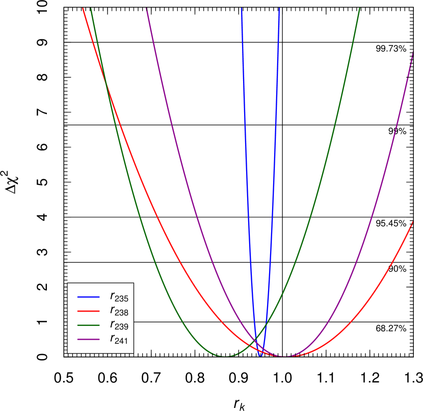
Figure 1: Marginal $\Delta\chi^{2}_{\text{R}}=\chi^{2}_{\text{R}}-(\chi^{2}_{\text{R}})_{\text{min}}$ for the coefficients $r_{k}$ of the four antineutrino fluxes obtained from the fit of the reactor rates.

The fit of the data gives $(\chi^{2}_{\text{R}})_{\text{min}}=17.7$ with $22$ degrees of freedom, which correspond to an excellent $72\%$ goodness of fit. Figure 1 shows the marginal $\Delta\chi^{2}_{\text{R}}=\chi^{2}_{\text{R}}-(\chi^{2}_{\text{R}})_{\text{min}}$ for the coefficients $r_{k}$ of the four antineutrino fluxes, for which we obtain:

$$r_{235}=\hbox{} \hbox{}0.950\pm 0.014,$$ (3)

$$r_{238}=\hbox{} \hbox{}1.009\pm 0.147,$$ (4)

$$r_{239}=\hbox{} \hbox{}0.869\pm 0.097,$$ (5)

$$r_{241}=\hbox{} \hbox{}1.005\pm 0.100.$$ (6)

These values and Fig. 1 are different from the corresponding ones in Ref. Giunti (2017), because of the different second term in Eq. (2) with respect to that in Eq. (8) of Ref. Giunti (2017), which constrained all the $r_{k}$’s. The best-fit values and uncertainties of $\sigma_{f,235}$ and $\sigma_{f,239}$ are given in the second column of Table 1. The value of $\sigma_{f,235}$ is determined by the fit with a precision of about $1.4\%$ and differs from the theoretical value $\sigma_{f,235}^{\text{SH}}$ by $2.0\sigma$. This confirms the necessity of a revaluation of the theoretical value of $\sigma_{f,235}$ found in Ref. Giunti (2017). The value of $\sigma_{f,239}$ is also determined by the fit, but with the worse precision of about $11.2\%$, which renders it compatible with the theoretical value $\sigma_{f,239}^{\text{SH}}$ within $1.3\sigma$.

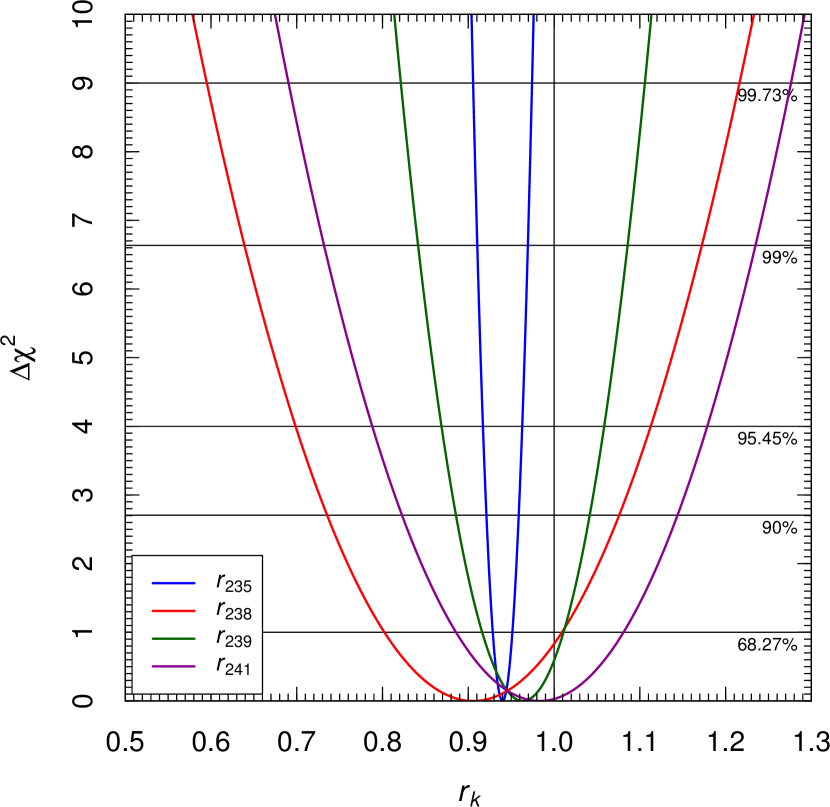
Figure 2: Marginal $\Delta\chi^{2}_{\text{tot}}=\chi^{2}_{\text{tot}}-(\chi^{2}_{\text{tot}})_{\text{min}}$ for the coefficients $r_{k}$ of the four antineutrino fluxes obtained from the fit of the reactor rates and the Daya Bay measurement of $\sigma_{f,235}$ and $\sigma_{f,239}$ An et al. (2017a).

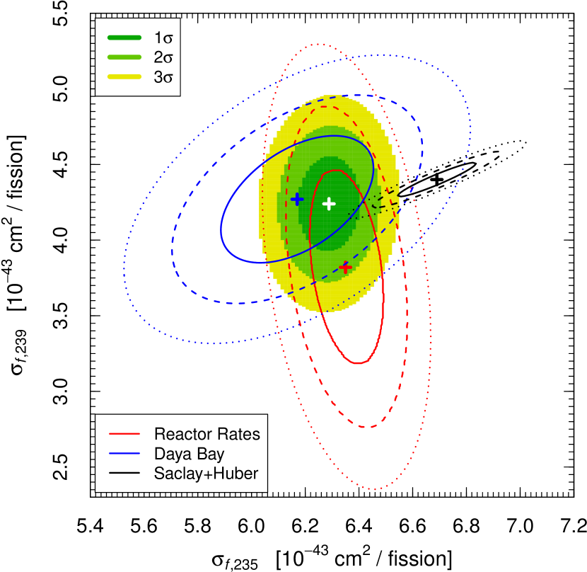
Figure 3: Allowed regions in the $\sigma_{f,235}$–$\sigma_{f,239}$ plane obtained from the combined fit of the reactor rates and the Daya Bay measurement of $\sigma_{f,235}$ and $\sigma_{f,239}$ An et al. (2017a). The red, blue and black curves enclose, respectively, the allowed regions obtained from the fit of the reactor rates, the allowed regions corresponding to the Daya Bay measurement of $\sigma_{f,235}$ and $\sigma_{f,239}$ An et al. (2017a), and the theoretical Saclay+Huber allowed regions at $1\sigma$ (solid), $2\sigma$ (dashed), and $3\sigma$ (dotted). The best-fit points are indicated by crosses.

In order to take into account the Daya Bay measurement of $\sigma_{f,235}$ and $\sigma_{f,239}$ An et al. (2017a), we consider the least-squares statistic

$$\hbox{}\chi^{2}_{\text{tot}}=\widetilde{\chi}^{2}_{\text{R}}$$

$$\hbox{}+\sum_{k,j=235,239}\left(\sigma_{f,k}^{\text{th}}-\sigma_{f,k}^{\text{DB}}\right)\left(V_{\text{DB}}^{-1}\right)_{kj}\left(\sigma_{f,j}^{\text{th}}-\sigma_{f,j}^{\text{DB}}\right),$$ (7)

where $\widetilde{\chi}^{2}_{\text{R}}$ is given by Eq. (2) without considering the Daya Bay rate An et al. (2017b), in order to avoid considering the Daya Bay data twice. The cross sections per fission $\sigma_{f,235}^{\text{DB}}$ and $\sigma_{f,239}^{\text{DB}}$ are those measured in Daya Bay An et al. (2017a) and listed in the third column of Table 1. We obtained the Daya Bay covariance matrix $V_{\text{DB}}$ with a Gaussian approximation of the $\chi^{2}$ distribution in Fig. 3 of Ref. An et al. (2017a). The theoretical cross sections per fission $\sigma_{f,k}^{\text{th}}$ are given by

$$\sigma_{f,k}^{\text{th}}=r_{k}\,\sigma_{f,k}^{\text{SH}},$$ (8)

with the same coefficients $r_{k}$ that are present in the definition of $R_{a}^{\text{th}}$ in Eq. (1).

The minimization of $\chi^{2}_{\text{tot}}$ gives $(\chi^{2}_{\text{tot}})_{\text{min}}=19.5$ with $23$ degrees of freedom, which correspond to a $67\%$ goodness of fit, which is practically as good as that obtained in the analysis of the reactor rates with $\chi^{2}_{\text{R}}$ in Eq. (2). Figure 2 shows the marginal $\Delta\chi^{2}_{\text{tot}}=\chi^{2}_{\text{tot}}-(\chi^{2}_{\text{tot}})_{\text{min}}$ for the coefficients $r_{k}$ of the four antineutrino fluxes, for which we obtain:

$$r_{235}=\hbox{} \hbox{}0.940\pm 0.011,$$ (9)

$$r_{238}=\hbox{} \hbox{}0.906\pm 0.103,$$ (10)

$$r_{239}=\hbox{} \hbox{}0.964\pm 0.047,$$ (11)

$$r_{241}=\hbox{} \hbox{}0.983\pm 0.097.$$ (12)

The corresponding best-fit values and uncertainties of $\sigma_{f,235}$ and $\sigma_{f,239}$ are given in the fourth column of Table 1. The value of $\sigma_{f,235}$ is determined by the fit with a precision which is slightly better than that obtained from the fit of the reactor rates, and significantly better than the precision of the Daya Bay measurement An et al. (2017a). The combined fit results in a substantial improvement of the precision of the determination of $\sigma_{f,239}$ with respect to the fit of the reactor rates alone: the value of $\sigma_{f,239}$ is determined with a precision of about $4.9\%$, which is also better than that of the Daya Bay measurement An et al. (2017a). Since the deviation from the theoretical value $\sigma_{f,239}^{\text{SH}}$ is only of $0.7\sigma$, there is no compelling necessity of a revaluation of its theoretical value.

Figure 3 shows the correlation between the determinations of $\sigma_{f,235}$ and $\sigma_{f,239}$. The values of $\sigma_{f,235}$ and $\sigma_{f,239}$ obtained from the fit of the reactor rates are slightly anticorrelated, whereas the Daya Bay values are significantly correlated and have a larger uncertainty for $\sigma_{f,235}$ and smaller uncertainty for $\sigma_{f,239}$. The combined fit results in an allowed region with practically uncorrelated values of $\sigma_{f,235}$ and $\sigma_{f,239}$ and significantly smaller uncertainties.

The $2.5\sigma$ deviation of $\sigma_{f,235}$ from the theoretical Saclay+Huber Mention et al. (2011); Huber (2011) cross sections per fission confirms the indications obtained in Refs. Giunti (2017); An et al. (2017a) that the reactor antineutrino anomaly is most probably mainly due to the ${}^{235}\text{U}$ electron antineutrino flux (if is not due to active-sterile neutrino oscillations). This possibility may be connected with a ${}^{235}\text{U}$ origin of the 5 MeV bump of the reactor antineutrino spectrum measured in the RENO Seo (2015); Choi et al. (2016), Double Chooz Abe et al. (2014), Daya Bay An et al. (2017b), and NEOS Ko et al. (2017) experiments, as indicated by the analysis in Ref. Huber (2017) and by the hint of a correlation in the RENO experiment Seo (2016). The new reactor experiments PROSPECT Ashenfelter et al. (2016), SoLid Ryder (2015), and STEREO Helaine which are in preparation for the search of short-baseline neutrino oscillations with highly enriched ${}^{235}\text{U}$ research reactors, will improve the determination of the ${}^{235}\text{U}$ electron antineutrino flux.

Since the ${}^{238}\text{U}$ and ${}^{241}\text{Pu}$ fuel composition in power reactors is small (see Table 1 of Ref. Gariazzo et al. (2017)), the antineutrino data do not give precise information on the corresponding cross sections per fission. From Fig. 2 one can see that $r_{238}=0.906\pm 0.103$ and $r_{241}=0.983\pm 0.097$. Hence, there is an indication that $\sigma_{f,238}$ may be substantially smaller than the theoretical $\sigma_{f,238}^{\text{SH}}$ value, but the discrepancy is less than $1\sigma$. On the other hand, the fit favors a value of $\sigma_{f,241}$ close to the theoretical $\sigma_{f,241}^{\text{SH}}$ value, but the uncertainty is large.

The calculations of the ${}^{235}\text{U}$, ${}^{239}\text{Pu}$, and ${}^{241}\text{Pu}$ antineutrino fluxes were performed through the inversion of the corresponding electron spectra measured at ILL in the 80’s Schreckenbach et al. (1985); Hahn et al. (1989). A possible explanation of the discrepancy between the calculated and measured values of $\sigma_{f,235}$ alone could be some unknown systematic error in the measurement of the ${}^{235}\text{U}$ electron spectrum which was not present in the measurements of the ${}^{239}\text{Pu}$ and ${}^{241}\text{Pu}$ electron electron spectra. It is clear that it would be very important to check these measurements with new experiments.

In conclusion, we performed a combined fit of the reactor antineutrino rates Giunti (2017) and the recent Daya Bay measurement of $\sigma_{f,235}$ and $\sigma_{f,239}$ An et al. (2017a). The combined fit leads to the better determination of $\sigma_{f,235}$ and $\sigma_{f,239}$ in Table 1, with respective uncertainties of about $1.2\%$ and $4.9\%$. The respective deviations from the theoretical Saclay+Huber Mention et al. (2011); Huber (2011) cross sections per fission are $2.5\sigma$ and $0.7\sigma$. Therefore, we confirm the conclusion already reached in Refs. Giunti (2017); An et al. (2017a) that the ${}^{235}\text{U}$ reactor antineutrino flux is the most probable main contributor to the reactor antineutrino anomaly Mention et al. (2011) if the anomaly is not due to active-sterile neutrino oscillations. However, also the ${}^{239}\text{Pu}$ flux, which is constrained by the cross section per fission in Table 1, and the ${}^{238}\text{U}$ and ${}^{241}\text{Pu}$ fluxes, for which the data do not provide stringent constraints, could be significantly different from the theoretical predictions. Let us finally emphasize that the knowledge of the reactor antineutrino fluxes is useful not only for applications in fundamental physics research, but also for practical applications as antineutrino monitoring of reactors (see Refs. Hayes et al. (2012); Christensen et al. (2014); Hayes (2017)).

References

- Mueller et al. (2011) T. A. Mueller et al., Phys. Rev. C83, 054615 (2011), arXiv:1101.2663 [hep-ex] .
- Huber (2011) P. Huber, Phys. Rev. C84, 024617 (2011), arXiv:1106.0687 [hep-ph] .
- Mention et al. (2011) G. Mention et al., Phys. Rev. D83, 073006 (2011), arXiv:1101.2755 [hep-ex] .
- Giunti (2017) C. Giunti, Phys.Lett. B764, 145 (2017), arXiv:1608.04096 [hep-ph] .
- An et al. (2017a) F. P. An et al. (Daya Bay), Phys.Rev.Lett. 118, 251801 (2017a), arXiv:1704.01082 [physics] .
- Gariazzo et al. (2017) S. Gariazzo, C. Giunti, M. Laveder, and Y. Li, JHEP 1706, 135 (2017), arXiv:1703.00860 [hep-ph] .
- Declais et al. (1994) Y. Declais et al. (Bugey), Phys. Lett. B338, 383 (1994).
- Kuvshinnikov et al. (1991) A. Kuvshinnikov, L. Mikaelyan, S. Nikolaev, M. Skorokhvatov, and A. Etenko, JETP Lett. 54, 253 (1991).
- Achkar et al. (1995) B. Achkar et al. (Bugey), Nucl. Phys. B434, 503 (1995).
- Zacek et al. (1986) G. Zacek et al. (CalTech-SIN-TUM), Phys. Rev. D34, 2621 (1986).
- Kwon et al. (1981) H. Kwon et al., Phys. Rev. D24, 1097 (1981).
- Hoummada et al. (1995) A. Hoummada, S. Lazrak Mikou, G. Bagieu, J. Cavaignac, and D. Holm Koang, Applied Radiation and Isotopes 46, 449 (1995).
- Vidyakin et al. (1987) G. S. Vidyakin et al. (Krasnoyarsk), Sov. Phys. JETP 66, 243 (1987).
- Vidyakin et al. (1990) G. S. Vidyakin et al. (Krasnoyarsk), Sov. Phys. JETP 71, 424 (1990).
- Vidyakin et al. (1994) G. S. Vidyakin et al. (Krasnoyarsk), JETP Lett. 59, 390 (1994).
- Afonin et al. (1988) A. I. Afonin et al., Sov. Phys. JETP 67, 213 (1988).
- Greenwood et al. (1996) Z. D. Greenwood et al., Phys. Rev. D53, 6054 (1996).
- Boireau et al. (2016) G. Boireau et al. (NUCIFER), Phys. Rev. D93, 112006 (2016), arXiv:1509.05610 [physics] .
- Apollonio et al. (2003) M. Apollonio et al. (CHOOZ), Eur. Phys. J. C27, 331 (2003), hep-ex/0301017 .
- Boehm et al. (2001) F. Boehm et al. (Palo Verde), Phys. Rev. D64, 112001 (2001), hep-ex/0107009 .
- An et al. (2017b) F. An et al. (Daya Bay), Chin.Phys. C41, 013002 (2017b), arXiv:1607.05378 [hep-ex] .
- Seo (2016) H. Seo, (2016), talk presented at AAP 2016, Applied Antineutrino Physics, 1-2 December 2016, Liverpool, UK.
- (23) Double Chooz Collaboration, Private Communication.
- Hayes and Vogel (2016) A. C. Hayes and P. Vogel, Ann.Rev.Nucl.Part.Sci. 66, 219 (2016), arXiv:1605.02047 [hep-ph] .
- Seo (2015) S.-H. Seo (RENO), AIP Conf. Proc. 1666, 080002 (2015), arXiv:1410.7987 [hep-ex] .
- Choi et al. (2016) J. Choi et al. (RENO), Phys. Rev. Lett. 116, 211801 (2016), arXiv:1511.05849 [hep-ex] .
- Abe et al. (2014) Y. Abe et al. (Double Chooz), JHEP 10, 086 (2014), [Erratum: JHEP 02, 074 (2015)], arXiv:1406.7763 [hep-ex] .
- Ko et al. (2017) Y. Ko et al. (NEOS), Phys.Rev.Lett. 118, 121802 (2017), arXiv:1610.05134 [hep-ex] .
- Huber (2017) P. Huber, Phys. Rev. Lett. 118, 042502 (2017), arXiv:1609.03910 [hep-ph] .
- Ashenfelter et al. (2016) J. Ashenfelter et al. (PROSPECT), J. Phys. G43, 113001 (2016), arXiv:1512.02202 [physics] .
- Ryder (2015) N. Ryder (SoLid), PoS EPS-HEP2015, 071 (2015), arXiv:1510.07835 [hep-ex] .
- (32) V. Helaine (STEREO), arXiv:1604.08877 [physics.ins-det] .
- Schreckenbach et al. (1985) K. Schreckenbach, G. Colvin, W. Gelletly, and F. Von Feilitzsch, Phys. Lett. B160, 325 (1985).
- Hahn et al. (1989) A. A. Hahn et al., Phys. Lett. B218, 365 (1989).
- Hayes et al. (2012) A. C. Hayes, H. R. Trellue, M. M. Nieto, and W. B. WIlson, Phys. Rev. C85, 024617 (2012), arXiv:1110.0534 [nucl-th] .
- Christensen et al. (2014) E. Christensen, P. Huber, P. Jaffke, and T. Shea, Phys. Rev. Lett. 113, 042503 (2014), arXiv:1403.7065 [physics] .
- Hayes (2017) A. C. Hayes, Rept. Prog. Phys. 80, 026301 (2017), arXiv:1701.02756 [nucl-th] .