Entanglement and the truncated moment problem

Abstract

We map the quantum entanglement problem onto the mathematically well-studied truncated moment problem. This yields a necessary and sufficient condition for separability that can be checked by a hierarchy of semi-definite programs. The algorithm always gives a certificate of entanglement if the state is entangled. If the state is separable, typically a certificate of separability is obtained in a finite number of steps and an explicit decomposition into separable pure states can be extracted.

I Introduction

The renewed interest that entanglement theory attracted in the last decades has led to a tremendous amount of new results (see the recent reviews [1, 2, 3, 4] and references therein). Still, characterization and detection of multipartite entanglement is largely an open question. For quantum states describing a collection of qubits, the size of Hilbert space, exponential in the number of qubits, makes the problem daunting. A simpler but still challenging problem is to restrict the question of characterizing entanglement to a smaller set of quantum states, such as for instance symmetric states, which are pure states invariant under permutations of constituents, or mixtures thereof. Symmetric states lie in a Hilbert space of size linear in the number of qubits, which makes the investigation more tractable. Once the symmetric case is understood, it can shed light onto the general case. This is the strategy we will follow here, first considering the symmetric case, which is easier to handle and to present from a pedagogical point of view, then extending our results to the fully general non-symmetric case.

Various results on entanglement for symmetric states have been obtained in the literature [5, 6, 7, 8, 9]. For instance, criteria for certifying separability in symmetric mixed states of $N$ qubits were found in [10]. Separable symmetric $N$-qubit pure states are always fully separable [11]. They are easily characterized, as there is a one-to-one correspondence between these states and points on the Bloch sphere via the Majorana representation [12]. As will be detailed in the paper, a symmetric state is separable (that is, it can be written as a convex combination of separable pure states) if and only if it can be associated with a probability distribution on the sphere; this measure then gives the positive weights associated with each separable pure state. A convenient representation to describe symmetric states in terms of symmetric tensors was proposed in [13], generalizing the Bloch sphere picture of spins-1/2. In terms of this tensor representation, decomposing a state into a convex combination of separable pure states amounts to finding a probability distribution whose lowest-order moments are fixed by the tensor entries. In fact, as we will see, the generic problem of finding whether an arbitrary (not necessarily symmetric) multipartite state can be decomposed into product states can be cast into the problem of finding a probability distribution whose lowest-order moments are fixed.

The problem of finding a probability distribution from the knowledge of its moments has been extensively studied in the literature. When only a finite number of moments is known, the problem is to find a probability distribution compatible with these moments. In the case of multivariate distributions, it corresponds to the so-called truncated moment problem: given a truncated moment sequence (tms), that is, fixing all moments up to a certain order, is there a probability distribution (or, in mathematical terms, a nonnegative measure) whose moments coincide with those of the tms? When it exists, such a measure is called a representing measure of the tms. Of practical relevance is the closely related $K$-tms problem, where the measure reproducing the fixed moments is constrained to be supported on some compact $K$.

The non-truncated $K$-moment problem, where all moments are given, was solved in [14] in the case where the compact $K$ is semi-algebraic (i.e. defined by polynomial inequalities). For the $K$-tms problem (and for $K$ semi-algebraic), Curto and Fialkow [15] obtained a necessary and sufficient condition for a tms to admit a representing measure (see Theorem 1 below). In [16], a semidefinite algorithm was introduced, allowing one to find a representing measure (if it exists), and later generalized to situations where only a subset of moments up to a certain order are known [17]. This algorithm was also used in [18] to test positivity of linear maps and separability of matrices in relation with the entanglement problem. More detail on the history of the tms problem can be found in the review [19].

The goal of the present paper is to show how the separability problem for an arbitrary quantum state can be mapped to the $K$-tms problem, and to use results from the tms literature to elucidate some aspects of entanglement detection and characterization of separability. From an analytical point of view, the mapping allows us to make use of theorems providing necessary and sufficient separability conditions. Numerically, semi-definite programming yields an algorithm to obtain an explicit decomposition of separable states.

The idea of using semi-definite programming to test for entanglement was already proposed in [20, 21, 22] by Doherty, Parrilo, and Spedalieri, and independently in [23]. In [21] an algorithm was provided which detects entanglement, but this algorithm never stops if the state is separable. Conversely, the algorithm proposed in [24] detects separable states but does not certify entanglement. The algorithms in [20, 21, 22] use the concept of “extensions”, i.e. states in a larger Hilbert space are considered, such that their partial trace gives back the original state. By going to larger and larger extensions, a hierarchy of semi-definite programs (SDPs) arises whose infeasability at any stage signals that the original state $\rho_{AB}$ is entangled. The authors of [20, 21, 22] add the request that the extensions have positive partial transpose (i.e. are “PPT”) as a necessary criterion for separability. This additional condition can be implemented at little extra cost in the SDP. Furthermore, they search in the space of “$N$ Bose-symmetric extensions”, where the extended state $\rho_{AB^{N}}$ (besides being positive semi-definite and reproducing $\rho_{AB}=\mathrm{tr}_{B^{N-1}}[\rho_{AB^{N}}]$) is invariant under projection onto the symmetric subspace of $B^{N}$. These algorithms were further improved in [25, 26, 27, 28].

The algorithm we propose here gives a unifying mathematical framework that also uses semi-definite programming and extensions, but in a somewhat more abstract way, based on a matrix of moments and a theorem in the theory of moment sequences. It provides an elegant solution of the entanglement problem, and in particular provides a certificate of separability, together with an explicit decomposition into product states if the state is separable. Moreover, it applies to arbitrary quantum state with arbitrary number of constituents and arbitrary symmetries between the subparts and easily accomodates missing data, i.e. incompletely specified states.

After setting up the notations, we define the $K$-tms problem (Section II), explain the procedures and algorithms allowing to solve it (Section III) and then show explicit numerical results (Section IV). In Section V we show that, conversely, some solutions of the entanglement problems may shed light on a particular tms problem. A discussion of the advantages and novelties of our treatment compared to previous algorithms is provided in the conclusions.

II Entanglement and the truncated moment problem

To familiarize the reader with the notations in this paper, we will first consider the case of symmetric states of qubits, since in this case the equations are more compact. After that we will explain the general case in the following subsection.

II.1 Symmetric qubit case

Multi-qubit pure states which are invariant under any permutation of the qubits are called symmetric pure states. Symmetric states are mixtures of symmetric pure states. Such states are formally equivalent to spin states with spin quantum number $N/2$, where $N$ is the number of qubits. This connection can be made explicit with the Dicke states defined by

$$|D_{N}^{(k)}\rangle=\mathcal{N}\sum_{\pi}|\underbrace{0\dots 0}_{k}\underbrace{1\dots 1}_{N-k}\rangle,$$ (1)

where $\mathcal{N}$ is a normalization constant and the sum runs over all permutations of the qubits. These states with $k\in\{0,\dots,N\}$ form a basis of the symmetric subspace of the Hilbert space $\mathbb{C}^{2^{N}}$ of $N$ qubits. We now introduce a convenient way of representing symmetric states as tensors. For a state $\rho$, let

$$X_{\mu_{1}\mu_{2}...\mu_{N}}=\mathrm{tr}\left\{\rho\,P^{\dagger}_{s}\sigma_{\mu_{1}}\otimes\cdots\otimes\sigma_{\mu_{N}}P_{s}\right\},$$ (2)

with $\sigma_{0}$ the $2\times 2$ identity matrix, $\sigma_{1},\sigma_{2},\sigma_{3}$ the three Pauli matrices, and $P_{s}$ the projector onto the symmetric subspace spanned by Dicke states (1). Then $\rho$ can be expanded [13] as

$$\rho=\frac{1}{2^{N}}X_{\mu_{1}\mu_{2}...\mu_{N}}P^{\dagger}_{s}\sigma_{\mu_{1}}\otimes\cdots\otimes\sigma_{\mu_{N}}P_{s}$$ (3)

(with summation over repeated indices). The tensor $X_{\mu_{1}\mu_{2}...\mu_{N}}$ is real and invariant under permutation of indices, and verifies

$$X_{0...0}=\mathrm{tr}\rho=1.$$ (4)

In this representation, the tensor associated with a pure separable symmetric state $|\psi_{sep}\rangle$ of $N$ qubits takes the particularly simple form

$$X_{\mu_{1}\mu_{2}...\mu_{N}}=n_{\mu_{1}}\cdots n_{\mu_{N}}$$ (5)

with $n_{0}=1$ and $\mathbf{n}=(n_{1},n_{2},n_{3})$ the Bloch vector of the individual qubit, $n_{1}^{2}+n_{2}^{2}+n_{3}^{2}=1$. Note that since the state is invariant under the exchange of qubits, a pure state can only be the tensor product of identical qubits (with same Bloch vector $\mathbf{n}$), and a separable pure symmetric state has to be fully separable [29]. As a consequence, a symmetric state is separable if and only if its tensor representation can be written as

$$X_{\mu_{1}\mu_{2}...\mu_{N}}=\sum_{j}w_{j}n_{\mu_{1}}^{(j)}\cdots n_{\mu_{N}}^{(j)},$$ (6)

with $w_{j}\geqslant 0$, $n_{0}^{(j)}=1$ and each Bloch vector $\mathbf{n}^{(j)}$ normalized to 1. This can be equivalently written in an integral form as

$$X_{\mu_{1}\mu_{2}...\mu_{N}}=\int_{K}x_{\mu_{1}}x_{\mu_{2}}\cdots x_{\mu_{N}}d\mu(\mathbf{x}),$$ (7)

with $K=\{\mathbf{x}\in\mathbb{R}^{3}:x_{1}^{2}+x_{2}^{2}+x_{3}^{2}=1\}$ the unit sphere, $x_{0}=1$, and $d\mu$ a positive measure on $K$. Indeed, if (6) holds then the tensor can be written as in (7) with

$$d\mu(\mathbf{x})=\sum_{j}w_{j}\delta(\mathbf{x}-\mathbf{n}^{(j)}).$$ (8)

Conversely, since the system is finite-dimensional, Carathéodory’s theorem implies that the integral in (7) can always be reduced to a finite sum as in (6), so that the positive measure can always be expressed as a sum of delta functions. Expressing Eq. (7) in words, a symmetric state is separable if and only if there exist a positive measure $d\mu$ such that all entries of the tensor $X_{\mu_{1}\mu_{2}...\mu_{N}}$ (for all $\mu_{j}$, $1\leqslant j\leqslant N$ and $0\leqslant\mu_{i}\leqslant 3$) are given by moments of that measure.

In order to prepare for the generalization to arbitrary states in the next subsection, let us introduce a more compact notation for Eq. (7). For any $N$-tuple $(\mu_{1},\ldots,\mu_{N})$ we define a triplet $\alpha=(\alpha_{1},\alpha_{2},\alpha_{3})$ of integers such that

$$x_{\mu_{1}}x_{\mu_{2}}\cdots x_{\mu_{N}}=x^{\alpha},$$ (9)

where we use the notation $x^{\alpha}=x_{1}^{\alpha_{1}}x_{2}^{\alpha_{2}}x_{3}^{\alpha_{3}}$. So e.g. for $\alpha=(1,3,0)$ we have $x^{\alpha}=x_{1}x_{2}^{3}$. The degree of the monomial $x^{\alpha}$ is denoted $|\alpha|\equiv\sum_{i}\alpha_{i}$. We also denote the $X_{\mu_{1}\mu_{2}...\mu_{N}}$ by $y_{\alpha}$, where $\alpha$ corresponds to $(\mu_{1}\mu_{2}...\mu_{N})$ via Eq. (9), so that e.g. for $N=6$, $y_{(2,1,0)}=X_{000112}$. With this notation we can rewrite (7) as

$$y_{\alpha}=\int_{K}x^{\alpha}d\mu(\mathbf{x}).$$ (10)

To test if a symmetric state is separable, a necessary and sufficient condition is therefore that a positive measure $d\mu$ exists that fulfills (10) for all $|\alpha|\leqslant N$. Problems of this type are known as truncated $K$-moment sequence problems (or $K$-tms problems), and they can be solved by a semi-definite relaxation procedure. Before we describe this method in Section III we generalize the description to arbitrary states of finite-dimensional systems.

II.2 General case

Consider a multipartite quantum state $\rho$ acting on the tensor product $\mathcal{H}=\mathcal{H}^{(1)}\otimes\mathcal{H}^{(2)}\otimes\cdots\otimes\mathcal{H}^{(d)}$ of Hilbert spaces $\mathcal{H}^{(i)}$. For each $i$, let $S_{\mu}^{(i)},0\leqslant\mu\leqslant t_{i}$ be a set of $t_{i}+1$ Hermitian matrices forming an orthogonal basis (with respect to the scalar product tr$A^{\dagger}B$) of the set of bounded linear operators on $\mathcal{H}^{(i)}$, with the choice that $S_{0}^{(i)}$ is the identity matrix. An orthogonal basis of $\mathcal{H}$ is then given by matrices

$$S_{\mu_{1}\mu_{2}\dots\mu_{d}}=S^{(1)}_{\mu_{1}}\otimes S^{(2)}_{\mu_{2}}\otimes\cdots\otimes S^{(d)}_{\mu_{d}}$$ (11)

and any state can be written as

$$\rho=\mathcal{N}X_{\mu_{1}\mu_{2}\ldots\mu_{d}}S_{\mu_{1}\mu_{2}\dots\mu_{d}}$$ (12)

where summation over repeated indices is understood, and the normalization constant $\mathcal{N}=\prod_{i=1}^{d}\mathcal{N}_{i}$, with $\mathcal{N}_{i}=1/\sqrt{t_{i}+1}$, is chosen so that $X_{0\ldots 0}=1$. A quantum state $\rho_{sep}$ is said to be separable (over that particular factorization of $\mathcal{H}$) if it can be written as

$$\rho_{sep}=\sum_{j}w_{j}\,\rho_{j}^{(1)}\otimes\rho_{j}^{(2)}\otimes\dots\otimes\rho_{j}^{(d)}$$ (13)

with $w_{j}\geqslant 0$, and $\rho_{j}^{(i)}$ density matrices acting on $\mathcal{H}^{(i)}$ [30]. Any $\rho^{(i)}$ acting on $\mathcal{H}^{(i)}$ can be expanded as $\rho^{(i)}=\mathcal{N}_{i}\sum_{\mu_{i}}y_{\mu_{i}}^{(i)}S_{\mu_{i}}^{(i)}$, with $y^{(i)}$ a real $(t_{i}+1)$-dimensional vector. The condition $\mathrm{tr}\rho^{(i)}=1$, together with the choice that $S_{0}^{(i)}$ is the identity matrix and the normalization, implies that $y_{0}^{(i)}=1$.

Rewriting condition (13) in terms of average values, we get that a state is fully separable if and only if all averaged basis operators can be expressed as

$$\langle S_{\mu_{1}\mu_{2}\dots\mu_{d}}\rangle_{\rho}=\sum_{j}w_{j}\langle S_{\mu_{1}}^{(1)}\rangle_{\rho_{j}^{(1)}}\langle S_{\mu_{2}}^{(2)}\rangle_{\rho_{j}^{(2)}}\cdots\langle S_{\mu_{p}}^{(d)}\rangle_{\rho_{j}^{(d)}}$$ (14)

with $w_{j}\geqslant 0$, i.e. the expectation values of all $S_{\mu_{1}\mu_{2}\dots\mu_{d}}$ are convex combinations of the product of local expectation values. This condition can be reexpressed in terms of the coefficients $X_{\mu_{1}\mu_{2}\ldots\mu_{d}}$ of $\rho_{sep}$ in the expansion (12) and the coefficients $y_{a_{i}}^{(i;j)}$, $1\leqslant a_{i}\leqslant t_{i}$, in the expansion $\rho_{j}^{(i)}=\mathcal{N}_{i}\sum_{\mu_{i}}y_{\mu_{i}}^{(i;j)}S_{\mu_{i}}^{(i)}$, with $y_{0}^{(i;j)}=1$. Separability is then equivalent to the existence of $w_{j}\geqslant 0$ and real numbers $y_{a_{i}}^{(i;j)}$, $1\leqslant a_{i}\leqslant t_{i}$, such that for all $\mu_{i}$ with $0\leqslant\mu_{i}\leqslant t_{i}$ one has

$$X_{\mu_{1}\mu_{2}\ldots\mu_{d}}=\sum_{j}w_{j}\,y_{\mu_{1}}^{(1;j)}y_{\mu_{2}}^{(2;j)}\cdots y_{\mu_{d}}^{(d;j)}$$ (15)

and $\sum_{\mu_{i}}y_{\mu_{i}}^{(i;j)}S_{\mu_{i}}^{(i)}\geqslant 0$ for all $i$ and $j$. This latter condition comes from the fact that each $\rho_{j}^{(i)}=\mathcal{N}_{i}\sum_{\mu_{i}}y_{\mu_{i}}^{(i;j)}S_{\mu_{i}}^{(i)}$ appearing in (13) is a density matrix, and thus has to be positive. Since matrices are Hermitian and thus have all their eigenvalues real, one can use Descartes sign rule to express this positivity condition as inequalities on the coefficients of the characteristic polynomial of $\rho_{j}^{(i)}$. Each of these coefficient is a linear combination of traces of powers of $\rho_{j}^{(i)}$, and therefore a polynomial in the variables $y_{\mu}^{(i;j)}$. Thus, each vector ${\bf y}^{(i;j)}=(y_{1}^{(i;j)},\ldots,y_{t_{i}}^{(i;j)})$ is restricted to a certain compact subset $K^{(i)}\subset\mathbb{R}^{t_{i}}$ defined by some polynomial inequalities, e.g. for a qubit the polynomial is a quadratic equation of the Bloch vector, restricting its maximal length to one. Defining the compact $K=K^{(1)}\times K^{(2)}\times\cdots\times K^{(d)}\subset\mathbb{R}^{n}$, $n=\sum_{i}t_{i}$, and the vector $\mathbf{y}^{(j)}=(\mathbf{y}^{(1;j)},\mathbf{y}^{(2;j)},\dots,\mathbf{y}^{(d;j)})\in\mathbb{R}^{n}$, the positivity condition on the partial density matrices amounts to impose that $\mathbf{y}^{(j)}\in K$ with $K$ a compact defined by polynomial inequalities. Equation (15) can then be rewritten, for $0\leqslant\mu_{i}\leqslant t_{i}$, as

$$X_{\mu_{1}\mu_{2}\dots\mu_{d}}=\int_{K}x_{\mu_{1}}^{(1)}x_{\mu_{2}}^{(2)}\cdots x_{\mu_{d}}^{(d)}d\mu(\mathbf{x})$$ (16)

with $x_{0}^{(i)}=1$, $\mathbf{x}=\left(\mathbf{x}^{(1)},\mathbf{x}^{(2)},\dots,\mathbf{x}^{(d)}\right)\in\mathbb{R}^{n}$, $\mathbf{x}^{(i)}=(x^{(i)}_{a})_{1\leqslant a\leqslant t_{i}}\in\mathbb{R}^{t_{i}}$, and $d\mu$ the measure over $\mathbb{R}^{n}$ defined by

$$d\mu(\mathbf{x})=\sum_{j}w_{j}\,\delta(\mathbf{x}-\mathbf{y}^{(j)}).$$ (17)

Equation (16) is the generalization of the symmetric case Eq. (7), the difference being that each Hilbert space $\mathcal{H}^{(i)}$ has its own set of variables $(x^{(i)}_{a})_{1\leqslant a\leqslant t_{i}}$. As in the symmetric case, the existence of an arbitrary measure $d\mu(\mathbf{x})$ such that (16) holds is equivalent to the existence of a ’discrete’ measure of the form (17), since one can apply Carathéodory’s theorem to our finite dimensional Hilbert spaces. The separability problem, for a state given by (12), is thus equivalent to the question whether a positive measure $d\mu$ with support $K$ exists whose moments coincide with the coordinates $X_{\mu_{1}\mu_{2}\dots\mu_{d}}$ of the state.

We now rewrite Eq. (16) in a more compact form. Let us relabel the entries of $\mathbf{x}$ as $\mathbf{x}=\left(x_{1},x_{2},\dots,x_{n}\right)$, and introduce the notation $x^{\alpha}\equiv\prod_{i=1}^{n}x_{i}^{\alpha_{i}}$, where $\alpha=(\alpha_{1},\alpha_{2},\dots,\alpha_{n})$ is a vector of integers. For instance for two qubits we have $\mathbf{x}=\left(x^{(1)}_{1},x^{(1)}_{2},x^{(1)}_{3},x^{(2)}_{1},x^{(2)}_{2},x^{(2)}_{3}\right)=(x_{1},x_{2},\dots,x_{6})$. For any given tuple $(\mu_{1},\dots,\mu_{d})$, there exists an index $\alpha$ such that

$$x_{\mu_{1}}^{(1)}x_{\mu_{2}}^{(2)}\cdots x_{\mu_{d}}^{(d)}=x^{\alpha}.$$ (18)

Thus, $\alpha_{1}$ counts the number of $x^{(1)}_{1}$ in the monomial $x_{\mu_{1}}^{(1)}x_{\mu_{2}}^{(2)}\cdots x_{\mu_{d}}^{(d)}$, $\alpha_{2}$ counts the number of $x^{(1)}_{2}$, and so on until $\alpha_{n}$, which counts the number of $x^{(d)}_{t_{d}}$. For instance for a bipartite state of $d=2$ qubits, $(\mu_{1},\mu_{2})=(2,3)$ corresponds to $\alpha=(0,1,0,0,0,1)$ or to the monomial $x_{2}^{(1)}x_{3}^{(2)}$, while $(\mu_{1},\mu_{2})=(1,0)$ corresponds to $\alpha=(1,0,0,0,0,0)$ or to the monomial $x_{1}^{(1)}$. As each monomial $x_{\mu_{1}}^{(1)}x_{\mu_{2}}^{(2)}\cdots x_{\mu_{d}}^{(d)}$ contains at most one variable of each type $x^{(i)}$, the vector $\alpha$ is such that each tuple $(\alpha_{1},\ldots,\alpha_{t_{1}})$, $(\alpha_{t_{1}+1},\ldots,\alpha_{t_{1}+t_{2}})$,$\ldots$, contains at most one 1. For instance for qubits, where $t_{i}=3$, each triplet $(\alpha_{3i+1},\alpha_{3i+2},\alpha_{3i+3})$ must therefore contain at most one 1.

If we denote $X_{\mu_{1}\mu_{2}\dots\mu_{d}}$ by $y_{\alpha}$, where $\alpha$ is the index corresponding to the tuple $(\mu_{1},\dots,\mu_{d})$ via (18), then Eq. (16) can be simply rewritten as

$$y_{\alpha}=\int_{K}x^{\alpha}d\mu(\mathbf{x}).$$ (19)

Hence, a state is separable if and only if all its coordinates $y_{\alpha}$ can be written as in Eq. (19), with $d\mu$ a positive measure.

II.3 Examples and special cases

The general setting of the previous Subsection allows one to test separability for a given fixed partition. For example, in order to check full separability for a three-qubit state $\rho$ one has to consider $d=3$ sets of variables $x^{(i)}_{a_{i}}$, each set being associated with a qubit (thus with $1\leqslant a_{i}\leqslant 3$), and $K$ is the product of three Bloch spheres. One then relabels the coordinates $X_{\mu_{1}\mu_{2}\mu_{3}}$ of $\rho$ as $y_{\alpha}$ and the variables as $(x_{1},\ldots,x_{n})$ with $n=9$, in order to get Eq. (19). Among all 9-tuples $\alpha=(\alpha_{1},\ldots,\alpha_{n})$, only the 64 values which correspond to some triplet $(\mu_{1},\mu_{2},\mu_{3})$ for $0\leqslant\mu_{i}\leqslant 3$ via (18) have to be considered. The state $\rho$ is separable if and only if there exists a measure $d\mu$ such that Eq. (19) is fulfilled for all these $\alpha$.

However if one is only interested in the question of entanglement of the first two qubits with respect to the third one, one would have to take the first two qubits as a 4-level system. There would then be two sets of variables in Eq. (16), the first one with $t_{1}=15$ variables (characterizing the density matrix of a 4-level system), and the second with $t_{2}=3$ variables (characterizing a mixed qubit state). Thus one has $d=2$ and $n=18$ variables. Finding whether or not (19) can be solved answers the question whether or not the third qubit is entangled with the first two, while ignoring any entanglement between the first two qubits.

It is instructive to see how the symmetric case of Subsection II.1 can be recovered from the general case. As we saw in Subsection II.1, the problem of finding whether a symmetric $N$-qubit state is fully separable can be cast into the form (10), with $K$ the 2-sphere and $\alpha$ running over triplets of integers with $|\alpha|\leqslant N$. Applying the general case to the $N$-qubit case implies $d=N$ parties, and the Hilbert space $\mathcal{H}$ is decomposed as $\mathcal{H}=\mathcal{H}^{(1)}\otimes\mathcal{H}^{(2)}\otimes\cdots\otimes\mathcal{H}^{(N)}$. Each Hilbert space $\mathcal{H}^{(i)}$ has its own set of variables $x^{(i)}_{a_{i}}$, $1\leqslant a_{i}\leqslant 3$, appearing in the right-hand side of Eq. (16). The basis $S_{\mu}^{(i)}$ in the decomposition $\rho^{(i)}=\frac{1}{2}\sum_{\mu}y_{\mu}^{(i)}S_{\mu}^{(i)}$ is the Pauli basis, the vectors $(y^{(i)}_{a})_{1\leqslant a\leqslant 3}$ are the Bloch vectors and the compact $K^{(i)}$ such that $\sum_{\mu}y_{\mu}^{(i)}S_{\mu}^{(i)}$ is positive is the Bloch ball. Symmetry then implies that the variables corresponding to each Hilbert space are not independent but equal, so that one has to require $x_{\mu}^{(i)}=x_{\mu}$ for all $i$ and $\mu$, and replace the compact $K^{(1)}\times K^{(2)}\times\cdots\times K^{(d)}$ by $K=K^{(1)}$, a single Bloch sphere. To account for the fact that the different sets of variables should no longer be distinguished, the $n$-tuple $\alpha$ in (19) should be replaced by the triplet $(\sum_{i}\alpha_{3i+1},\sum_{i}\alpha_{3i+2},\sum_{i}\alpha_{3i+3})$ giving the multiplicities of $x_{1},x_{2},x_{3}$. The entries of the triplet can now take values larger than one. Since Eq. (19) and Eq. (10) coincide, the symmetric and the general case are in essence the same problem; the difference between them lies only in the definition of the compact $K$ supporting the measure, and also in the set of tuples $\alpha$ considered.

The general formalism (19) allows us in fact to play with any kind of constraint, just by adjusting the sets of variables and $\alpha$ vectors accordingly. The symmetric case explained above is just one example, but this method is general. For instance if one wants to impose a symmetry between two of the subsystems one just has to equate the sets of independent variables. This adjustment can be easily generalized to test for entanglement for any type of partition. The algorithms for the truncated moment problem that we will present in Section III provide a solution to all these cases.

II.4 Partial knowledge of a state

An interesting question in practical application is whether or not a partial set of measurement results is compatible with a separable state. If for example a state tomography is not carried to its end, or if only local measurements are available, can one in some instances infer that the state was entangled? Another interesting question is whether the partial traces of a state can be used to show entanglement of the global state even if all the reduced states are separable [31].

Such problems of partial knowledge can be formulated in the form of Eq. (19) very simply. The only change is the range of tuples over which $\alpha$ varies: since the unknown measurements correspond to unknown $y_{\alpha}$, these values of $\alpha$ should not be taken into account as constraints on $d\mu$. If for example only the results of local measurements are known, only averages of the form $\langle S^{(1)}_{0}\otimes S^{(2)}_{0}\otimes\cdots S^{(i)}_{\mu}\cdots\otimes S^{(d)}_{0}\rangle$ are known (recall that $S^{(i)}_{0}$ is the identity matrix). Therefore one only knows the values of $y_{\alpha}$ such that the $\alpha=(\alpha_{1},\dots,\alpha_{n})$ have only one non-zero entry. This problem can then be solved in the same way as the general one, just by putting no constraint on the unknown moments.

III TMS Problems: definitions and solutions

Identifying the entanglement problem with the $K$-tms problem allows us to use analytical results and numerical methods from the tms literature to get insight in entanglement theory. We now introduce the mathematical formalism used to describe and solve the tms problem.

III.1 Truncated moment problems

A truncated moment sequence (tms) of degree $d$ is a finite set of numbers $y=(y_{\alpha})_{|\alpha|\leqslant d}$ indexed by $n$-tuples $\alpha=(\alpha_{1},\ldots,\alpha_{n})$ of integers $\alpha_{i}\geqslant 0$ such that $|\alpha|=\sum_{i}\alpha_{i}\leqslant d$ [17]. The truncated $K$-moment problem consists in finding conditions under which there exists a (positive) measure $d\mu$ such that each moment $y_{\alpha}$ with $|\alpha|\leqslant d$ can be represented as an integral of the form

$$y_{\alpha}=\int_{K}x^{\alpha}d\mu(\mathbf{x})$$ (20)

with $\mathbf{x}=(x_{1},\ldots,x_{n})\in\mathbb{R}^{n}$, $x^{\alpha}=x_{1}^{\alpha_{1}}x_{2}^{\alpha_{2}}\ldots x_{n}^{\alpha_{n}}$, and $d\mu$ a measure supported on a semi-algebraic set

$$K=\{\mathbf{x}\in\mathbb{R}^{n}|g_{1}(\mathbf{x})\geqslant 0,\cdots,g_{m}(\mathbf{x})\geqslant 0\}$$ (21)

with $g_{i}(\mathbf{x})$ multivariate polynomials in the variables $x_{1},\ldots,x_{n}$. If such a measure exists it can be written as the sum of delta functions

$$d\mu(\mathbf{x})=\sum_{j=1}^{r}w_{j}\delta\left(\mathbf{x}-\mathbf{y}^{(j)}\right)$$ (22)

with some finite $r$, $w_{j}>0$ and $\mathbf{y}^{(j)}\in K$. Such a measure is then called a finitely atomic representing measure. Equation (20) is nothing but Eq. (10), where $K$ is the Bloch sphere, $d=N$, and $n=3$. Therefore the entanglement problem for symmetric states is a special case of $K$-tms problem.

The $\mathcal{A}K$-tms problem [17] is a generalization of the $K$-tms problem in which moments $y_{\alpha}$ are known only for a finite subset $\mathcal{A}\subset\mathbb{N}^{n}$ of indices of degree $|\alpha|\leqslant d$. The only difference with the $K$-tms problem is that Eq. (20) now has to be fulfilled only for $\alpha\in\mathcal{A}$. This is exactly the situation found in the general case of Subsection II.2. Indeed, in that case, we showed that $K$ is defined by polynomial inequalities, so that it is a semi-algebraic compact set. Moreover, only indices $\alpha$ associated with some tuple $(\mu_{1},\dots,\mu_{d})$ for $0\leqslant\mu_{i}\leqslant t_{i}$ do correspond to a certain moment $y_{\alpha}$, so that a restriction on indices $\alpha$ is required. This is also the situation encountered in Subsection II.4, where the state is only known partially. All these cases therefore correspond to the $\mathcal{A}K$-tms problem, and can in fact be solved in the same way as the $K$-tms problem, only with fewer constraints (since less moments are fixed).

In all what follows, to ease notations, we will only treat the original $K$-tms problem where all moments $y_{\alpha}$ with $|\alpha|\leqslant d$ are known. However, we must stress that the $\mathcal{A}K$-tms problem is treated in exactly the same way, just by considering $\alpha\in\mathcal{A}$ rather than $|\alpha|\leqslant d$ in all equations involving that restriction.

III.2 Moment matrices

Let us now present the mathematical setting for the $K$-tms problem defined by Eq. (20). Let $y=(y_{\alpha})_{|\alpha|\leqslant d}$ be a tms of degree $d$, with $\alpha=(\alpha_{1},\ldots,\alpha_{n})$ being $n$-tuples of integers. The integrand in the right-hand side of Eq. (20) is a monomial in $n$ variables $(x_{1},\ldots,x_{n})$ of degree less than $d$. Any polynomial of degree less than $d$ can be written as a vector in the basis of monomials ordered in degree-lexicographic order (that is, monomials are sorted by order and within each order in a lexicographic order). For instance for $n=3$ and $d=2$ the monomial basis is $\{1,x_{1},x_{2},x_{3},x_{1}^{2},x_{1}x_{2},x_{1}x_{3},x_{2}^{2},x_{2}x_{3},x_{3}^{2}\}$, and a polynomial such as e.g. $p(\mathbf{x})=7x_{3}-3x_{2}^{2}+2$ would be written as the vector $(2,0,0,7,0,0,0,-3,0,0)$. The components of the vector representing $p(\mathbf{x})$ are coefficients $p_{\alpha}$ such that $p(\mathbf{x})=\sum_{\alpha}p_{\alpha}x^{\alpha}$.

For any integer $k\leqslant d/2$, let $M_{k}(y)$ be the matrix defined by

$$M_{k}(y)_{\alpha\beta}=y_{\alpha+\beta},\qquad|\alpha|,|\beta|\leqslant k.$$ (23)

It is called the moment matrix of order $k$ associated with the tms $y$. A necessary condition for a tms to admit a representing measure as in (20) is that the moment matrix of any order is positive-semidefinite. Indeed, if (20) holds, then for any vector $p=(p_{\alpha})_{|\alpha|\leqslant k}$ representing a polynomial $p(\mathbf{x})$ of degree $k$ or less we have

$$p^{T}M_{k}(y)p=\sum_{|\alpha|,|\beta|\leqslant k}p_{\alpha}y_{\alpha+\beta}p_{\beta}=\hfill$$

$$\hfill\sum_{|\alpha|,|\beta|\leqslant k}p_{\alpha}p_{\beta}\int_{K}x^{\alpha+\beta}d\mu(\mathbf{x})=\int_{K}p(\mathbf{x})^{2}d\mu(\mathbf{x})\geqslant 0,$$ (24)

so that $M_{k}(y)$ a is positive-semidefinite matrix [15, 16].

Other necessary conditions can be obtained from the polynomial constraints $g_{i}(\mathbf{x})\geqslant 0$ which define the set $K$ in (21). For any polynomial $g$ of degree $\text{deg}(g)\geqslant 1$, one can define a ’shifted tms’ of degree $d-\text{deg}(g)$ as

$$(g\star y)_{\alpha}=\sum_{|\gamma|\leqslant deg(g)}g_{\gamma}y_{\alpha+\gamma},\quad|\alpha|\leqslant d-\text{deg}(g).$$ (25)

Let $d_{g}=\lceil\text{deg}(g)/2\rceil$ (we denote by $\lceil x\rceil$ the smallest integer larger than $x$ and by $\lfloor x\rfloor$ the largest integer smaller than $x$). Applying definition (23), one can define the $(k-d_{g})$th moment matrix of $g\star y$, for any integer $k$ such that $0\leqslant k-d_{g}\leqslant[d-\text{deg}(g)]/2$, by $M_{k-d_{g}}(g\star y)_{\alpha\beta}=(g\star y)_{\alpha+\beta}$. This matrix is called the $k$th-order localizing matrix of $g$ [16]. In explicit form, it reads

$$M_{k-d_{g}}(g\star y)_{\alpha\beta}=\sum_{|\gamma|\leqslant deg(g)}g_{\gamma}y_{\alpha+\beta+\gamma},\quad |\alpha|,|\beta|\leqslant k-d_{g}.$$ (26)

Using the fact that $\lfloor(d-\text{deg}(g))/2\rfloor=\lfloor d/2\rfloor-d_{g}$, we have that the $k$th-order localizing matrix is defined for any integer $k$ such that $d_{g}\leqslant k\leqslant d/2$ (the definition of $d_{g}$ has been precisely chosen in such a way that the upper bound $k\leqslant d/2$ is the same as that for the $k$th-order moment matrix). If a tms admits a representing measure then any $k$th order localizing matrix is necessarily positive-semidefinite: indeed for any vector $p=(p_{\alpha})_{|\alpha|\leqslant k-d_{g}}$ representing a polynomial $p(\mathbf{x})$ with degree $k-d_{g}$ or less we have

$$p^{T}M_{k-d_{g}}(g\star y)p =\sum_{|\alpha|,|\beta|\leqslant k-d_{g}}p_{\alpha}p_{\beta}\sum_{|\gamma|\leqslant deg(g)}g_{\gamma}y_{\alpha+\beta+\gamma}$$

$$=\int_{K}g(\mathbf{x})p(\mathbf{x})^{2}d\mu(\mathbf{x})\geqslant 0,$$ (27)

which is positive because $g$ is positive on $K$ by the definition (21). Another way of seing that is to observe that if $y$ admits a positive representing measure then so does the shifted tms $g\star y$.

As moment matrices of order $k^{\prime}$ are submatrices of matrices of order $k$ if $k^{\prime}\leqslant k$ it suffices to consider the largest possible value for $k$ to get the strongest necessary conditions. For a tms $y$ of order $d$, the above analysis leads to the necessary condition $M_{\lfloor d/2\rfloor}(y)\geqslant 0$. If the compact $K$ is defined as in (21) by polynomial inequalities, the localizing matrices for each polynomial $g_{i}$, $1\leqslant i\leqslant m$, have to be positive, namely $M_{\lfloor d/2\rfloor-d_{g_{i}}}(g_{i}\star y)\geqslant 0$, $d_{g_{i}}=\lceil\text{deg}(g_{i})/2\rceil$.

III.3 A necessary and sufficient condition

The above conditions are only necessary conditions. A sufficient condition was obtained in [15] for even-order tms. We formulate it following Theorem 1.1 of [16]. Namely, if a tms $z$ of even order $2k$ is such that its $k$th order moment matrix and all $k$th order localizing matrices are positive, and if additionally

$$\mbox{rank}M_{k}(z)=\mbox{rank}M_{k-d_{0}}(z)$$ (28)

with $d_{0}=\max_{1\leqslant i\leqslant m}\{1,\lceil\mbox{deg}(g_{i})/2\rceil\}$, then the tms $z$ admits a representing measure composed of $r=\mbox{rank}M_{k}(z)$ delta functions. Note that the rank condition already appeared in [25] under the name rank-loop, using a result from [32].

As the above condition is only sufficient, a tms $y$ admitting a representing measure does not necessarily fulfill (28). However, one can search for an extension $z$ of $y$ which fulfills it. An extension of a tms $y$ of degree $d$ is defined as any tms $z$ of degree $2k$ with $2k>d$, such that $z_{\alpha}=y_{\alpha}$ for all $|\alpha|\leqslant d$. A extension $z$ is called flat if it satisfies Eq. (28). If $z$ verifies the sufficient conditions above, then it has a representing measure, and so does $y$ as a restriction of $z$. This allows us to formulate the following necessary and sufficient condition for the existence of a representing measure.

Theorem 1 ([15] (see also Theorem 1.2 of [16])).

A tms $(y_{\alpha})_{|\alpha|\leqslant d}$ admits a representing measure supported by $K$ if and only if there exists a flat extension $(z_{\beta})_{|\beta|\leqslant 2k}$ with $2k>d$ such that $M_{k}(z)\geqslant 0$, and $M_{k-d_{g_{i}}}(g_{i}\star z)\geqslant 0$ for $i=1,\ldots,m$.

This theorem can be implemented as a semi-definite program, as shown in Section III.4. It has been extended to an abritrary $\mathcal{A}$K-tms in proposition 3.3 in [17]. With the identifications made in Sec.II between the entanglement and the tms problem, these results can be reformulated as a necessary and sufficient condition for separability of an arbitrary quantum state:

Theorem 2.

A state $\rho$ is separable if and only if its coordinates $X_{\mu_{1}\mu_{2}\dots\mu_{d}}$ defined in (12) correspond to a tms $(y_{\alpha})_{\alpha\in\mathcal{A}}$ such that there exists a flat extension $(z_{\beta})_{|\beta|\leqslant 2k}$ with $2k>d$, $M_{k}(z)\geqslant 0$, and $M_{k-d_{g_{i}}}(g_{i}\star z)\geqslant 0$ for $i=1,\ldots,m$.

III.4 Semi-definite program and the entanglement problem

For a given tms $(y_{\alpha})_{|\alpha|\leqslant d}$, finding a extension $(z_{\beta})_{|\beta|\leqslant 2k}$ as in the theorem above amounts to constructing a positive matrix $M_{k}(z)_{\alpha\beta}=z_{\alpha+\beta}$ with some entries given, namely $z_{\alpha}=y_{\alpha}$ for $|\alpha|\leqslant d$, and constraints of positivity of moment matrices and localizing matrices, which are linear in the $z_{\alpha}$. This type of problem corresponds to what is known in numerical analysis as semi-definite program (SDP) problems. Here, the variables of the SDP are the $z_{\beta}$ for $|\beta|\leqslant 2k$. The smallest extension order is $k_{0}=\lfloor d/2\rfloor+1$. All the constraints of Theorem 1 can be directly implemented in the SDP apart from the flatness condition (28). If also the flatness condition could be implemented efficiently then $P=NP$ [19]. To take into account the flatness condition, the idea [17] is to consider the SDP

$$\min_{z}\sum_{\alpha,|\alpha|\leqslant k_{0}}R_{\alpha}z_{\alpha}\quad\mbox{such that}$$ (29)

$$M_{k}(z)\geqslant 0$$ (30)

$$M_{k-d_{i}}(g_{i}\star z)\geqslant 0\quad\textrm{for }i=1,\ldots,m$$ (31)

$$z_{\alpha}=y_{\alpha}\,\,\mbox{for}\,|\alpha|\leqslant d.$$ (32)

The coefficients $R_{\alpha}$ are chosen randomly, but in order to ensure that $\sum_{\alpha,|\alpha|\leqslant k_{0}}R_{\alpha}z_{\alpha}$ has indeed a global minimum, the polynomial $R(\mathbf{x})=\sum_{\alpha}R_{\alpha}x^{\alpha}$ is taken as a sum-of-squares polynomial of degree $2k_{0}$. When the order of the extension $k$ is increased, the polynomial is kept the same, so that minimization is realized only on the $z_{\beta}$ with $|\beta|\leqslant 2k_{0}$.

According to the theorems above, finding a representing measure, or finding a decomposition into a mixture of separable product states, amounts to finding an extension $z$ that fulfills the constraints (30)–(32), i.e. such that the SDP is "feasible", and that also fulfills the rank condition (28). We can now propose an algorithm which, for any entangled state, provides a certificate of entanglement, and for a separable state usually halts at the first iteration $k=k_{0}$ and provides a decomposition into pure product states. This algorithm is illustrated in Fig. 1. One runs the algorithm by starting from the lowest possible extension order $k=k_{0}$ and increasing $k$. If there exists an order $k$ such that the SDP is infeasible, then the tms $y$ admits no representing measure. In terms of entanglement, this means that the quantum state whose coordinates are given by the $y_{\alpha}$ is entangled. If, on the contrary, the SDP problem is feasible at some order $k$ (i.e. if all constraints can be met) and if for that value of $k$ the extension obtained fulfills (28), then the tms $y$ admits a representing measure, and the corresponding quantum state is separable with respect to the multipartite factorization of Hilbert space considered. The algorithm remains inconclusive as long as the SDP remains feasible but with an extension which is not flat. In such a case, one can either repeat the SDP with the same $k$ and a different $R$, or increase the order $k$ by one. As soon as the rank condition is met, or the SDP becomes infeasible, the algorithm stops and gives a certificate of separability, or entanglement. The only situation where the algorithm does not give an answer in a finite number of steps is the case where extensions are found for any $k$ and all choices of $R$, but are never flat.

When the algorithm stops with a feasible flat extension $z$ it is possible to extract a representing measure as a sum of rank[$M_{k}(z)$] delta functions [16], which provides an explicit factorization of the separable quantum state. Indeed, suppose the algorithm stops at order $k$ and gives an extension $z=z^{*}$ which optimizes (29) and fulfills the rank condition (28). If the moment matrix of the optimal solution $M_{k}(z^{*})$ has rank $r$, then it is possible to calculate an explicit decomposition of the form

$$M_{k}(z^{*})_{\alpha\beta}=\sum_{j=1}^{r}w_{j}\,x^{*}(j)^{\alpha}x^{*}(j)^{\beta},\quad|\alpha|,|\beta|\leqslant k,$$ (33)

with $w_{j}\geqslant 0$, $\sum_{j}w_{j}=1$, and $\mathbf{x}^{*}(j)\in K$, with the methods described in [33] and implemented in the Matlab package Gloptipoly 3 [34] (see Appendix A). These $r$ vectors yield $r$ delta functions in the decomposition of the representing measure, and for a separable quantum state they yield an explicit decomposition as a sum of $r$ factorized states.

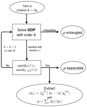
Figure 1: Flow diagram to visualize the algorithm. ”Solve SDP” refers to (29)-(32)

IV Implementation and numerical results

IV.1 Two-qubit symmetric states

We now apply this tms approach to some concrete examples of entanglement detection, starting with the simplest case of two-qubit symmetric states. Any state $\rho$ can be expanded as in Eq. (3) with $N=2$. The tms problem is given by (10) with $d=N=2$ and $n=3$ variables. We can choose to obtain a decomposition of the state either into mixed states, in which case the compact $K$ should be taken as the unit ball, or into pure states, where $K$ has to be the unit sphere. Here we consider the pure state decomposition, so that we define $K=\{\mathbf{x}\in\mathbb{R}^{3}|g(\mathbf{x})=0\}$ with $g(\mathbf{x})=x_{1}^{2}+x_{2}^{2}+x_{3}^{2}-1$ (equality $g(x)=0$ obviously means that $K$ is semi-algebraic and defined by the two polynomials $g\geqslant 0$ and $-g\geqslant 0$). The measure $d\mu$ must satisfy constraints such as

$$y_{110}=\int_{||\mathbf{x}||=1}x_{1}x_{2}d\mu(\mathbf{x})\quad\mbox{or}\quad y_{002}=\int_{||\mathbf{x}||=1}x_{3}^{2}d\mu(\mathbf{x})\,$$ (34)

where $||\mathbf{x}||^{2}=x_{1}^{2}+x_{2}^{2}+x_{3}^{2}$ and the $y_{\alpha}$ are the entries corresponding to the $X_{\mu_{1}\mu_{2}}$.

The necessary condition given in Subsection III.2 is positivity of the moment matrix of order $d/2=1$, that is, $M_{1}(y)\geqslant 0$, with

$$M_{1}(y)=\left(\begin{array}[]{cccc}y_{000}&y_{100}&y_{010}&y_{001}\\ y_{100}&y_{200}&y_{110}&y_{101}\\ y_{010}&y_{110}&y_{020}&y_{011}\\ y_{001}&y_{101}&y_{011}&y_{002}\\ \end{array}\right).$$ (39)

Solving the entanglement problem in this case amounts to constructing a tms $(z_{\beta})_{|\beta|\leqslant 2k}$ which is a flat extension of $y$. Since $k_{0}=2$, the lowest-order moment matrix of the extension is $M_{2}(z)$, which is a $10\times 10$ matrix whose upper left $4\times 4$ block is the matrix (39). The conditions of Theorem 2 imply that we look for an extension such that $M_{2}(z)\geqslant 0$ and $M_{1}(g*z)\geqslant 0$, where

$$M_{1}(g*z)=\left(\begin{array}[]{cccc}z_{000}-z_{200}-z_{020}-z_{002}&z_{100}-z_{300}-z_{120}-z_{102}&z_{010}-z_{210}-z_{030}-z_{012}&z_{001}-z_{201}-z_{021}-z_{003}\\ z_{100}-z_{300}-z_{120}-z_{102}&z_{200}-z_{400}-z_{220}-z_{202}&z_{110}-z_{310}-z_{130}-z_{112}&z_{101}-z_{301}-z_{121}-z_{103}\\ z_{010}-z_{210}-z_{030}-z_{012}&z_{110}-z_{310}-z_{130}-z_{112}&z_{020}-z_{220}-z_{040}-z_{022}&z_{011}-z_{211}-z_{031}-z_{013}\\ z_{001}-z_{201}-z_{021}-z_{003}&z_{101}-z_{301}-z_{121}-z_{103}&z_{011}-z_{211}-z_{031}-z_{013}&z_{002}-z_{202}-z_{022}-z_{004}\\ \end{array}\right)$$ (44)

is the $4\times 4$ localizing matrix of $z$. The SDP is then to find $\min_{z}\sum_{\alpha}R_{\alpha}z_{\alpha}$, with $R$ an arbitrary given list of coefficients so that $\sum_{\alpha}R_{\alpha}z_{\alpha}$ is positive and bounded, under the constraints that $M_{2}(z)\geqslant 0$, $M_{1}(g*z)\geqslant 0$ and $z_{\alpha}=y_{\alpha}$ for $|\alpha|\leqslant 2$.

The point of this subsection was to illustrate the different ingredients of our algorithm. In fact, in this case, the necessary condition $M_{1}(y)\geqslant 0$ is necessary and sufficient. Indeed, $M_{1}(y)$ is exactly the $4\times 4$ matrix $(X_{\mu\nu})_{0\leqslant\mu,\nu\leqslant 3}$, which was proven in [29] to be similar to the partial transpose matrix of $\rho$ up to a factor 1/2. It is well-known that the partial transpose criterion is a necessary and sufficient separability condition for two qubits [35, 36], hence positivity of $M_{1}(y)$ suffices to prove separability.

In Theorem 4.7 of [37] the authors solved the $K$-tms problem of degree 2 in the case where $K$ is defined by a single quadratic equality, by direct proof rather than using the above theorems on generic tms. The key point is a result from [38]. Applying this theorem to a tms $y$ of degree 2 when $K$ is a sphere, the necessary and sufficient conditions for $y$ to admit a representing measure are $M_{1}(y)\leqslant 0$ and $y_{000}-y_{200}-y_{020}-y_{002}=0$. Using the mapping between the tms problem and the separability problem, this theorem of [37] directly yields the necessary and sufficient condition $M_{1}(y)\geqslant 0$ mentioned above for separability of a symmetric two-qubit state (the condition $y_{000}-y_{200}-y_{020}-y_{002}=0$ being fulfilled for any symmetric two-qubit state). Actually, this problem also coincides with problem of characterizing the convex hull of spin coherent states. For spin-1, a necessary and sufficient criterion was established in terms of positivity of a matrix [39]. Again, this criterion can be shown to coincide with the condition $M_{1}(y)\geqslant 0$. Moreover, it was shown in [40] that any separable symmetric two-qubit state could be decomposed as a mixture of four pure product states. The tms approach provides a concise constructive proof of the same fact, as we show in Appendix B.

States \$N$	2	3	4	5	6	7	8	9	10	11	12
$\rho_{ent}$	0.2	0.2	0.4	0.6	1.0	2.1	5.2	11.6	26.8	54.6	170.5
$\rho_{sep}$	0.7	0.4	0.6	1.0	2.0	4.2	10.2	20.8	66.9	94.5	716.3

Table 1: Timing of the algorithm in seconds for $N$-qubit symmetric states as function of $N$, averaged over 100 random states, when run on a standard desktop PC. The first row corresponds to random states drawn from the uniform Haar measure (following [41]), which are usually entangled. They are typically detected by the condition $M_{k}(y)\geqslant 0$. The second row corresponds to random separable states created by randomly mixing random pure separable states. The timing can vary depending on the separable state tested and the randomly generated functional $R$ in (29). Up to six different $R$ are tested before moving to the next order.

IV.2 $N$-qubit symmetric states

The case of an $N$-qubit symmetric state $\rho$ can be mapped onto the tms problem of Eq. (10) where $\mathbf{x}=(x_{1},x_{2},x_{3})$ is a vector of $\mathbb{R}^{3}$. We define $K=\{x\in\mathbb{R}^{3}|g(\mathbf{x})=0\}$, with $g(\mathbf{x})=x_{1}^{2}+x_{2}^{2}+x_{3}^{2}-1$ as in the two-qubit case. The highest degree of the monomial $x^{\alpha}$ in (10) is the total number of indices of the tensor $X_{\mu_{1}\ldots\mu_{N}}$, i.e. $d=N$. The degree of the polynomial defining $K$ is 2, and therefore $d_{0}=1$.

To numerically investigate the algorithm for an $N$-qubit symmetric state we have to solve a SDP with degree $d=N$ and flatness condition rank$M_{k}(z)=$rank$M_{k-1}(z)$. If the state is entangled ($\rho_{ent}$) the SDP (29)–(32) should prove infeasible at some value of $k$, but this usually happens already at the lowest order $k=k_{0}$. When the state is separable ($\rho_{sep}$) the algorithm has to find a flat extension for some $k$, which may require to run the SDP for more than one $R$, or to increase the values of $k$. Hence, the run time is typically longer than in the case of an entangled state, as can be seen in Table 1. Usually we found a flat extension either at the lowest order $k=k_{0}$ or at order $k=k_{0}+1$.

IV.3 Physical interpretation of the positivity of $M_{k}(y)$

Consider a $2k$-qubit symmetric state $\rho$. The necessary condition $M_{k}(y)\geqslant 0$ of Sec.III.2 turns out to be equivalent to the positivity of the partial transpose of $\rho$ with respect to the $k$ first qubits. Indeed, let $T$ be the real symmetric matrix defined by

$$T_{\boldsymbol{\mu},\boldsymbol{\nu}}=X_{\mu_{1}\dots\mu_{k}\nu_{1}\ldots\nu_{k}}$$ (45)

in terms of the coordinates $X_{\mu_{1}\mu_{2}...\mu_{2k}}$ of $\rho$ [see Eq. (3)], where matrix indices $\boldsymbol{\mu}$ and $\boldsymbol{\nu}$ are multi-indices $\boldsymbol{\mu}=(\mu_{1},\ldots,\mu_{k})$ and $\boldsymbol{\nu}=(\nu_{1},\ldots,\nu_{k})$, with $0\leqslant\mu_{i},\nu_{i}\leqslant 3$. Then, up to a constant numerical factor, the matrix $T$ is similar to the partial transpose of the density matrix in the computational basis for the partition into two sets of $k$ qubits each [29]. Moreover, $T$ has some recurring rows and columns, which when removed yield exactly the moment matrix $M_{k}(y)$. A symmetric matrix is positive semi-definite if and only if all principal minors, i.e. the determinant of all submatrices, are non-negative. The determinant of a matrix which has a recurring column or row is equal to zero, so only the submatrices with non-recurring rows and columns have to be considered. Therefore, $T$, and thus the partial transpose, is positive semi-definite if and only if the matrix $M_{k}(y)$ is positive semi-definite. So the necessary condition $M_{k}(y)\geqslant 0$ is equivalent to the positive partial transpose criterion of a symmetric state of $2k$-qubits with equal size partitions. Since for a separable $N$-qubit state $\rho$ any reduced density matrix of $2k$ qubits has to be separable, the necessary conditions $M_{k}(y)\geqslant 0$ with $k\leqslant N/2$ can be interpreted as positivity of the partial transpose of the reduced density matrices of $\rho$. This provides an interesting interpretation of the physical meaning of the positivity of the moment matrix.

IV.4 Minimal number of pure product states needed

If a quantum state is separable it can be written as a convex sum of product states. Replacing each product state by its eigenvalue-eigenvector decomposition we obtain a decomposition of the initial quantum state as a convex sum of pure product states. What is the minimal number $r_{\textrm{min}}$ of pure product states required to decompose an arbitrary separable state?

The answer is unknown in the general case. For symmetric states, pure states in the decomposition have to be symmetric themselves (see e.g. Theorem 1 in [29]). As the appendix B shows, and as was obtained in [40], in the case of two qubits, four states are sufficient to represent any separable symmetric state.

The above algorithm yields rank$M_{k}(z)=r$ as an upper bound to the number of pure states required to decompose a given quantum state. In order to investigate systematically the number of states required, we generated symmetric separable states by mixing a large number $m$ of random separable symmetric pure states with random weights as

$$\rho_{\textrm{sep,sym}}=\sum_{i=1}^{m}w_{i}\left(|\psi_{i}\rangle\langle\psi_{i}|\right)^{\otimes N},$$ (46)

with $\sum_{i}w_{i}=1$, and applied the algorithm to the resulting mixed states. When our algorithm stops with a flat extension $z$ such that rank$M_{k}(z)=r$, then $r$ is an upper bound on the true minimal number of separable states required to express $\rho_{\textrm{sep,sym}}$. Indeed, since the extension depends on the random choice of $R_{\alpha}$ there may be extensions with a smaller rank, as the algorithm does not minimize this rank. Therefore every number $r<m$ obtained should give an upper bound to the actual generic value for $r_{\textrm{min}}$. In practice we generated a large list of separable symmetric states with a value of $m=25$ for $N\leqslant 6$ and $m=45$ for $N>6$ and found a flat extension for each one. The smallest numbers found are reported in Table 2.

$N$	Min $r$	# min	States tested
2	4	37304	61494
3	6	2410	60641
4	9	1104	174011
5	12	17	174193
6	17	408	153081
7	22	18	16129
8	29	12	16030
9	35	2	10000
10	42	1	10000

Table 2: The smallest value of $r$ found, which gives an upper bound on the true value $r_{\textrm{min}}$ of the maximal number of pure states needed to generate every separable symmetric state. In the third column, # min gives the number of states for which the value min $r$ has been reached among the states tested.

V A new solution to a particular tms problem

The mapping presented above not only helps solving the separability problem, but it can also, conversely, shed light on particular tms problems by using results from entanglement theory. We now give an example of such a situation.

One of the best-known results from entanglement theory is the Peres-Horodecki criterion, which states that $2\times 2$ and $2\times 3$ systems are separable if and only if the partial transpose is positive [35, 36] (PPT-criterion). It has been generalized to the following two statements: If $\rho$ is supported on $\mathbb{C}^{2}\times\mathbb{C}^{N}$ and the rank $r(\rho)=N$ then $\rho$ is separable (Theorem 1 of [42]) and can be written as a convex sum of projectors on $N$ product vectors (Corollary 3a of [42]).

When $\rho$ is fully symmetric, the above characterizations yield the following result:

Theorem 3 ([43]).

Let $\rho$ be a symmetric $N$-qubit state with positive partial transpose with respect to the first qubit. If $N=2$ or $3$, or if $N>3$ and $r(\rho)\leqslant N$, then $\rho$ is fully separable.

Note that for four qubits there exist entangled symmetric states with a positive partial transpose [44]. As shown in [29], the PPT conditions can be expressed as linear matrix inequalities involving the entries of the tensor $X_{\mu_{1}\mu_{2}\ldots\mu_{N}}$, or equivalently the $y_{\alpha}$. Rewriting the above theorem for $N=3$ in the language of $K$-tms problems, this yields a theorem for a special case of a tms. Even more, by using the fact that $2\times 3$ systems are separable if and only if they are PPT, we directly get a necessary and sufficient condition for a tms problem of degree $d=3$ to admit a representing measure supported on the unit sphere of $\mathbb{R}^{3}$. This condition reads

$$\left(\begin{array}[]{cccccccc}y_{000}+y_{001}&y_{100}-\mathrm{i}y_{010}&y_{100}+y_{101}&y_{200}-\mathrm{i}y_{110}&y_{010}+y_{011}&y_{110}-\mathrm{i}y_{020}&y_{001}+y_{002}&y_{101}-\mathrm{i}y_{011}\\ y_{100}+\mathrm{i}y_{010}&y_{000}-y_{001}&y_{200}+\mathrm{i}y_{110}&y_{100}-y_{101}&y_{110}+\mathrm{i}y_{020}&y_{010}-y_{011}&y_{101}+\mathrm{i}y_{011}&y_{001}-y_{002}\\ y_{100}+y_{101}&y_{200}-\mathrm{i}y_{110}&y_{200}+y_{201}&y_{300}-\mathrm{i}y_{210}&y_{110}+y_{111}&y_{210}-\mathrm{i}y_{120}&y_{101}+y_{102}&y_{201}-\mathrm{i}y_{111}\\ y_{200}+\mathrm{i}y_{110}&y_{100}-y_{101}&y_{300}+\mathrm{i}y_{210}&y_{200}-y_{201}&y_{210}+\mathrm{i}y_{120}&y_{110}-y_{111}&y_{201}+\mathrm{i}y_{111}&y_{101}-y_{102}\\ y_{010}+y_{011}&y_{110}-\mathrm{i}y_{020}&y_{110}+y_{111}&y_{210}-\mathrm{i}y_{120}&y_{020}+y_{021}&y_{120}-\mathrm{i}y_{030}&y_{011}+y_{012}&y_{111}-\mathrm{i}y_{021}\\ y_{110}+\mathrm{i}y_{020}&y_{010}-y_{011}&y_{210}+\mathrm{i}y_{120}&y_{110}-y_{111}&y_{120}+\mathrm{i}y_{030}&y_{020}-y_{021}&y_{111}+\mathrm{i}y_{021}&y_{011}-y_{012}\\ y_{001}+y_{002}&y_{101}-\mathrm{i}y_{011}&y_{101}+y_{102}&y_{201}-\mathrm{i}y_{111}&y_{011}+y_{012}&y_{111}-\mathrm{i}y_{021}&y_{002}+y_{003}&y_{102}-\mathrm{i}y_{012}\\ y_{101}+\mathrm{i}y_{011}&y_{001}-y_{002}&y_{201}+\mathrm{i}y_{111}&y_{101}-y_{102}&y_{111}+\mathrm{i}y_{021}&y_{011}-y_{012}&y_{102}+\mathrm{i}y_{012}&y_{002}-y_{003}\\ \end{array}\right)\geqslant 0.$$ (47)

(see the expression of [29] which explicitly gives the PPT criterion for 3 qubits). This result does not appear to have been known previously in the tms literature.

While (47) is a necessary and sufficient condition in the case of a tms of degree $N=3$, Theorem 3 also provides us with a sufficient condition for a tms of arbitrary degree $N$. Indeed, suppose one wants to know whether a given tms $y$ of degree $N>3$ admits a representing measure on the unit sphere. Using the mapping inverse to the one in Sec.IV.2 one can construct the density matrix $\rho$ associated with the tms via (3). If $\rho$ is PPT and has rank $r(\rho)\leqslant N$, then there exists a representing measure.

VI Conclusions

We have proposed a new and elegant solution of the entanglement problem by mapping it to the truncated $K$-moment problem. Benefiting from the mathematically well-developed field of the theory of moments, we provide an algorithm that for an entangled state certifies its entanglement in a finite number of steps. If the state is separable, it usually halts at the first iteration ($k=k_{0}$ in Fig.1) and then returns an explicit decomposition of the state into a convex sum of product states. Similarly to previous algorithms, our algorithm makes use of semi-definite programming and “extensions”, but there are a number of conceptual differences that allow us express and solve the problem very elegantly and adapt it easily to different physical situations, including subsystems of different dimensions or symmetries, or incomplete data.

In our approach, rather than working directly with the density matrix, the semi-definite optimization problem is based on moment matrices and localizing matrices, where the latter incorporate the constraints of the states of the sub-spaces. This is possible since these states in the sub-spaces are restricted to compact sets characterized by polynomial constraints (e.g. to Bloch spheres in the case of individual spins-1/2). Both the moment matrix and the localizing matrices must be positive semi-definite for a state to be separable. Extensions are extensions of the moment matrix, and we need not impose a particular symmetry on such an extension, nor positivity of the partial transpose of the state, since this is taken care of by positivity of the moment matrix (see Sec.IV.3).

Our algorithm contains in addition a crucial element, namely the idea of “flat extensions”: if at a given order $k$ of the extension the SDP is feasible, one checks whether the rank of the extended moment matrix is the same as the one at order $k-d_{0}$ [with $d_{0}$ related to the largest degree of the constraint polynomials, see after eq.(28)]. If so, the state is separable and one obtains its explicit convex decomposition into product states. In [25] it was already noted that when PPT is imposed on the extensions in the algorithm by Doherty et al. [20, 21, 22], sometimes separability can be concluded in a finite number of steps by checking whether the rank of the found extension of the density matrix has not increased compared to the original state, a situation called “rank loop”. There, the sufficiency of a rank loop for separability follows from a theorem due to Horodecki et al. [32], according to which a PPT state is separable if its rank is smaller or equal than the rank of the reduced state. In our case, the implementation of the flat-extension query is a decisive part of the algorithm, based on Theorem 1.

Formulating the entanglement as a truncated $K$-tms problem also has the advantage that the algorithm readily accepts incomplete data from an experiment. Indeed, since for multi-partite systems fully determining the state requires an effort that grows exponentially with the number of subsystems, fully specifying or experimentally determining the state becomes at some point impossible in practice. Since our algorithm is based from the very beginning on a truncated sequence of moments (that can be chosen to be expectation values of Hermitian operators that were measured), we can leave open additional moments that were not measured and still run the algorithm. Using the algorithm in this way should allow one to determine how many and which moments one should measure in order to still be able to prove that a state is entangled.

Finally, as symmetric states of $N$ qubits coincide with spin-$j$ states with $N=2j$, separable symmetric states can be identified with classical spin-$j$ states (see e.g. [39]). The latter, defined in [39], are convex combinations of spin-coherent states, and can be considered the quantum states which are closest to having a classical behaviour in the sense of minimal quantum fluctuations [45, 13, 29]. Applying the algorithm presented here to symmetric states of $N$-qubits also allows one to check whether a spin-$j$ state is classical.

Appendix A Matlab implementation

Here we give a Matlab implementation of the easiest case of the symmetric state of two qubits, (or a spin-1 state [46]). The quantum state $\rho$ is given as in (2) as

$$X_{\mu_{1}\mu_{2}}=\mathrm{tr}\{\rho\,P^{\dagger}_{s}\sigma_{\mu_{1}}\otimes\sigma_{\mu_{2}}P_{s}\},$$ (48)

with $P_{s}$ the projector onto the symmetric states. The following implementation uses Matlab and the programs GloptiPoly 3 [34] and the solver SeDuMi [47]. To increase the probability of finding a flat extension, the semi-definite solver should use the highest possible accuracy in the calculation of the minimal value of the SDP.

⬇

1mpol x 3

2xMom=[1 x(1) x(2) x(3) x(1)^2 x(1)*x(2) x(1)*x(3) x(2)^2 x(2)*x(3) x(3)^2];

3y=[X(1,1) X(1,2) X(1,3) X(1,4) X(2,2) X(2,3) X(2,4) X(3,3) X(3,4) X(4,4)];

4con=[mom(xMom)==y];

5K = [x(1)^2+x(2)^2+x(3)^2-1==0];

6G = randn(length(xMom));

7R = xMom*(G’*G)*xMom’; k=2;

8P = msdp(min(mom(R)),K,con,k);

9pars.eps=0; mset(pars);

10[status] =msol(P);

Line 3 is given by Eq. (48). Line 4 corresponds to Eq.(10). K fixes the variables to Bloch vectors of length 1. R is the arbitrary positive bounded polynomial which should be minimized. At line 8, ’msdp’ formulates the problem in the language of SDPs (construction of moment matrices and localizing matrices). Line 9 sets the accuracy of the SDP solver to its highest value. At line 10, ’msol’ solves the SDP.

• If the problem is detected as infeasible (status=-1) the state is entangled.

• If there is no flat extension found (status=0), one can re-run the program with a different R, or increase the order by one.

• If the state is separable and a flat extension is found (status=1) the solution can be extracted with the command "sol=double(x)". Then "sol" contains a list of Bloch vectors of the pure states that give a decomposition into separable states as in Eq. (6). The vector of weights $w_{i}$ can then be easily calculated.

This implementation can be extended to a larger number of qubits by adapting the monomial basis in line 2 to a higher degree and line 3 to contain all entries of the tensor $X_{\mu_{1}\ldots\mu_{N}}$ (Eq. (2)). The generalization to non-symmetric states is also possible, but the number of variables increases. E.g. two qubits would require one independent Bloch vector for each subsystem, so one would need six variables in total.

Appendix B Minimal rank for symmetric two-qubit states

Theorem 4.7 of [37] states that a tms $y$ of degree 2 admits a representing measure supported by $K$ if and only if $M_{1}(y)$ is positive and $y_{000}-y_{200}-y_{020}-y_{002}=0$. We therefore obtain that a two-bit symmetric state $\rho$ is separable if and only if it is associated with a tms such that $M_{1}(y)$ is positive and $y_{000}-y_{200}-y_{020}-y_{002}=0$. These two conditions in fact coincide respectively with the PPT criterion (see Sec.IV.3) and with the condition that $X_{00}=\sum_{a=1}^{3}X_{aa}$. The latter condition itself is a consequence of properties of the projections of tensor products of Pauli matrices over the symmetric subspace, as was shown in [13].

The proof of the fact that iff $M_{1}(y)$ is positive and $y_{000}-y_{200}-y_{020}-y_{002}=0$ then $\rho$ is separable into a mixture of only 4 separable states can be simplified by using the tms formalism. Let us derive the necessary and sufficient condition above in our language. The ’necessary’ direction is obvious. The proof for the ’sufficient’ direction goes as follows. Let us assume that the coordinates $X_{\mu\nu}$ form a positive rank-$r$ matrix $M_{1}(y)$. Since the state is symmetric, $M_{1}(y)$ is a real symmetric 4$\times$ 4 matrix and hence $r\leq 4$. Then $M_{1}(y)$ can be decomposed into a sum of $r$ projectors on orthogonal vectors $u^{(k)}$ as

$$X_{\mu\nu}=\sum_{k=1}^{r}u^{(k)}_{\mu}u^{(k)}_{\nu}.$$ (49)

Let $\Delta_{u}=(u_{0})^{2}-\sum_{a=1}^{3}(u_{a})^{2}$ for any 4-vector $u$. Since $X_{\mu\nu}$ verify $X_{00}=\sum_{a=1}^{3}X_{aa}$ we have $\sum_{i=1}^{r}\Delta_{u^{(i)}}=0$. Whenever $\Delta_{u^{(i)}}=0$, one has $u^{(i)}_{0}\neq 0$ (otherwise the whole vector $u^{(i)}$ vanishes and does not contribute to the sum (49)), so that the corresponding projector can be rewritten

$$u^{(i)}_{\mu}u^{(i)}_{\nu}=\left(u^{(i)}_{0}\right)^{2}n^{(i)}_{\mu}n^{(i)}_{\nu}$$ (50)

with $n^{(i)}=(1,{\bf n})$ and $|{\bf n}|=1$. If all $\Delta_{u^{(i)}}=0$ then Eqs. (49)–(50) immediately yield a sum over $r$ separable pure states. If not, then since $\sum_{i}\Delta_{u^{(i)}}=0$ there must be two indices $i$ and $j$ with $\Delta_{u^{(i)}}<0$ and $\Delta_{u^{(j)}}>0$. Let $v(t)=tu^{(i)}+(1-t)u^{(j)}$. Then $\Delta_{v(0)}>0$ and $\Delta_{v(1)}<0$, so that there has to be a $t_{c}\in]0,1[$ such that $\Delta_{v(t_{c})}=0$. The vector $v^{\prime}(t)=-(1-t)u^{(i)}+tu^{(j)}$ is then such that

$$u^{(i)}_{\mu}u^{(i)}_{\nu}+u^{(j)}_{\mu}u^{(j)}_{\nu}=\frac{v(t_{c})_{\mu}v(t_{c})_{\nu}+v^{\prime}(t_{c})_{\mu}v^{\prime}(t_{c})_{\nu}}{t_{c}^{2}+(1-t_{c})^{2}}.$$ (51)

Then subtracting a projector on $v(t_{c})$ yields

$$X_{\mu\nu}-\frac{v(t_{c})_{\mu}v(t_{c})_{\nu}}{t_{c}^{2}+(1-t_{c})^{2}}=\sum_{k=1}^{r-1}\tilde{u}^{(k)}_{\mu}\tilde{u}^{(k)}_{\nu}$$ (52)

where $\tilde{u}^{(k)}$ are the orthogonal states $u^{(k^{\prime})}$ ($k^{\prime}\neq i,j$) and $v^{\prime}(t_{c})$. Because of the definition of $t_{c}$ and using (50), the projector on $v(t_{c})$ is proportional to a projector representing a separable pure state, and the remaining sum is such that $\sum_{k=1}^{r-1}\Delta_{\tilde{u}^{(k)}}=0$. We are therefore back to the form (49) but with the rank reduced by one. The same procedure can be applied repeatedly to further reduce the rank down to 1; the last projector is then necessarily of the form (50). In the end, $\rho$ is written as a sum of $r\leqslant 4$ projectors on separable pure states.

References

- [1] D. Bruss, J. Math. Phys. 43, 4237 (2002).
- [2] M. B. Plenio and S. Virmani, Quantum Inf. Comput. 7, 1 (2007).
- [3] R. Horodecki, P. Horodecki, M. Horodecki, and K. Horodecki, Rev. Mod. Phys. 81, 865 (2009).
- [4] Otfried Gühne and Gèza Tóth, Phys. Rep. 474, 1 (2009).
- [5] A. R. U. Devi, R. Prabhu, and A. K. Rajagopal, Phys. Rev. Lett. 98, 060501 (2007).
- [6] R. Hübener, M. Kleinmann, T.-C. Wei, C. González-Guillén, and O. Gühne, Phys. Rev. A 80, 032324 (2009).
- [7] G. Tóth and O. Gühne, Phys. Rev. Lett. 102, 170503 (2009).
- [8] R. Augusiak, J. Tura, J. Samsonowicz, and M. Lewenstein, Phys. Rev. A 86, 042316 (2012).
- [9] D. Baguette, T. Bastin, and J. Martin, Phys. Rev. A 90, 032314 (2014).
- [10] E. Wolfe and S. F. Yelin, Phys. Rev. Lett. 112, 140402 (2014).
- [11] T. Ichikawa, T. Sasaki, I. Tsutsui, and N. Yonezawa, Phys. Rev. A 78, 052105 (2008).
- [12] E. Majorana, Nuovo Cimento 9, 43 (1932).
- [13] O. Giraud, D. Braun, D. Baguette, T. Bastin, and J. Martin, Phys. Rev. Lett. 114, 080401 (2015).
- [14] K. Schmüdgen, Math. Ann. 289, 203 (1991).
- [15] R. E. Curto and L. A. Fialkow, J. Operator Theory 54, 189 (2005).
- [16] J. W. Helton and J. Nie, Found. Comput. Math. 12, 851 (2012).
- [17] J. Nie, Found. Comput. Math. 14, 1243 (2014).
- [18] J. Nie and X. Zhang, SIAM J. Optim. 26, 1236 (2016).
- [19] M. Laurent, in Emerging Applications of Algebraic Geometry, edited by M. Putinar and S. Sullivant (Springer New York, 2009), pp. 157-270.
- [20] A. C. Doherty, P. A. Parrilo, and F. M. Spedalieri, Phys. Rev. Lett. 88, 187904 (2002).
- [21] A. C. Doherty, P. A. Parrilo, and F. M. Spedalieri, Phys. Rev. A 69, 022308 (2004).
- [22] A.C. Doherty, P.A. Parrilo, and F.M. Spedalieri, Phys. Rev. A 71, 032333 (2005).
- [23] J. Eisert, P. Hyllus, O. Gühne, and M. Curty, Phys. Rev. A 70, 062317 (2004).
- [24] F. Hulpke and D. Bruß, J. Phys. A: Math. Gen. 38, 5573 (2005).
- [25] M. Navascués, M. Owari, and M. B. Plenio, Phys. Rev. A 80, 052306 (2009).
- [26] B. Jungnitsch, T. Moroder, and O. Gühne, Phys. Rev. Lett. 106, 190502 (2011).
- [27] A. W. Harrow, A. Natarajan, and X. Wu, X. Commun. Math. Phys. 352, 881 (2017).
- [28] J. Chen, Z. Ji, D. Kribs, N. Lütkenhaus, and B. Zeng, Phys. Rev. A 90, 032318 (2014).
- [29] F. Bohnet-Waldraff, D. Braun, and O. Giraud, Phys. Rev. A 94, 042343 (2016).
- [30] R. F. Werner, Phys. Rev. A 40, 4277 (1989).
- [31] N. Miklin, T. Moroder, and O. Gühne, Phys. Rev. A 93, 020104 (2016).
- [32] P. Horodecki, M. Lewenstein, G. Vidal, and I. Cirac, Phys. Rev. A 62, 032310 (2000).
- [33] D. Henrion and J.-B. Lasserre, in Positive Polynomials in Control, edited by D. Henrion and A. Garulli (Springer Berlin Heidelberg, 2005), pp. 293-310.
- [34] D. Henrion, J. B. Lasserre and J. Loefberg, Optim. Methods Softw. 24, 761 (2009); see also http://homepages.laas.fr/henrion/software/gloptipoly/.
- [35] A. Peres, Phys. Rev. Lett. 77 , 1413 (1996).
- [36] M. Horodecki, P. Horodecki, and R. Horodecki, Phys. Lett. A 223, 1 (1996).
- [37] L. Fialkow and J. Nie, J. Funct. Anal. 258, 328 (2010).
- [38] J. Sturm and S. Zhang, Math. Oper. Res. 28, 246 (2003).
- [39] O. Giraud, P. Braun, and D. Braun, Phys. Rev. A 78, 042112 (2008).
- [40] M. Kuś and I. Bengtsson, Phys. Rev. A 80, 022319 (2009).
- [41] K. Życzkowski, K. A. Penson, I. Nechita, and B. Collins, J. Math. Phys. 52, 062201 (2011).
- [42] B. Kraus, J. I. Cirac, S. Karnas, and M. Lewenstein, Phys. Rev. A 61, 062302 (2000).
- [43] K. Eckert, J. Schliemann, D. Bruss, and M. Lewenstein, Ann. Phys.299, 88 (2002).
- [44] J. Tura, R. Augusiak, P. Hyllus, M. Kuś, J. Samsonowicz, and M. Lewenstein, Phys. Rev. A 85, 060302(R) (2012).
- [45] O. Giraud, P. Braun, and D. Braun, Phys. Rev. A 85, 032101 (2012).
- [46] F. Bohnet-Waldraff, D. Braun, and O. Giraud, Phys. Rev. A 93, 012104 (2016).
- [47] J. Sturm, Optim. Meth. Softw. 11, 625, 1999.