Mitigating Interference in Content Delivery Networks by Spatial Signal Alignment: The Approach of Shot-Noise Ratio

Abstract

Multimedia content especially videos is expected to dominate data traffic in next-generation mobile networks. Caching popular content at the network edge, namely content helpers (base stations and access points), has emerged to be a solution for low-latency content delivery. Compared with the traditional wireless communication, content delivery has a key characteristic that many signals coexisting in the air carry identical popular content. However, they can interfere with each other at a receiver if their modulation-and-coding (MAC) schemes are adapted to individual channels following the classic approach. To address this issue, we present a novel idea of content adaptive MAC (CAMAC) where adapting MAC schemes to content ensures that all signals carry identical content are encoded using an identical MAC scheme to achieve spatial MAC alignment. Consequently, interference can be harnessed as signals to improve the reliability of wireless delivery. In the remaining part of the paper, we focus on quantifying the gain that CAMAC can bring to a content-delivery network by using a stochastic-geometry model. Specifically, content helpers are distributed as a Poisson point process and each of them transmits a file from a content database based on a given popularity distribution. Given a fixed threshold on the signal-to-interference ratio for successful transmission, it is discovered that the successful content-delivery probability is closely related to the distribution of the ratio of two independent shot noise processes, named a shot-noise ratio. The distribution itself is an open mathematical problem that we tackle in this work. Using stable-distribution theory and tools from stochastic geometry, the distribution function is derived in closed form. Extending the result in the context of content-delivery networks with CAMAC yields the content-delivery probability in different closed forms. In addition, the gain in the probability due to CAMAC is shown to grow with the level of skewness in the content popularity distribution.

I Introduction

Videos and other types of multimedia data are becoming increasingly dominant in mobile traffic and undergoing exponential growth. This gives next-generation mobile networks a key mission of supporting low-latency and reliable content delivery. It is widely agreed that caching popular content at content helpers (e.g. base stations and access points) at the network edge is a promising solution. In this context, the paper presents a novel algorithm for efficient content delivery, called content adaptive modulation-and-coding (CAMAC). The algorithm aligns the modulation-and-coding (MAC) schemes used by content helpers to allow users to retrieve useful content from interference. Furthermore, we analyze the performance of a content-delivery network adopting CAMAC using a stochastic geometry model. In the process, an open problem concerning the distribution of the ratio of two shot noise processes is solved.

I-A Techniques for Content Caching and Delivery

Under the constraint that helpers have finite storage, efficient content delivery requires the joint design of the techniques for content caching and delivery. One approach called coded caching, is to jointly encode content cached at multiple helpers such that the broadcast nature of wireless transmission can be exploited for efficient content delivery by reducing the number of channel usages [1, 2]. Another approach does not involve coding and focus solely on optimizing the content placement at multiple helpers to reduce delivery latency. Solving the problem of optimal content placement was found to be NP-hard [3, 4]. Thus, most research based on the current approach aims at designing sub-optimal techniques using diversified tools such as greedy algorithms[3] and belief-propagation [4]. A survey of recent advancements in this direction can be found in [5].

In this work, we propose a new approach for efficient content delivery from the perspective of adaptive MAC. In classic communication theory, the MAC scheme is adapted to the channel state for coping with channel fading [6, 7]. In contrast, the proposed CAMAC design is to adapt MAC to the transmitted content file. The design is motivated by the fact that in a content-delivery system, many coexisting signals in the air carry the same popular content. Then CAMAC ensures all such signals are encoded using an identical MAC scheme, allowing them to combine at any intended/unintended receivers instead of interfering with each other. In other words, CAMAC represents a low-cost cooperative scheme for content helpers without message passing between them. The design effectively coordinates all helpers into a content-broadcast system.

I-B Modeling and Designing Content-Delivery Networks

The design and analysis of large-scale content-delivery networks is currently a highly active area. The research in the area focuses on designing strategies for caching content at helpers with finite storage so as to optimize the network performance. Stochastic-geometric network models are commonly adopted in this area where content helpers are typically distributed as Poisson point process (PPP). Correspondingly, the network performance is measured by the product of hit probability [8], defined as the probability that a file requested by a typical user is available at the associated helper and the content-delivery probability, defined as the probability that a transmitted file is received by an intended user with a signal-to-interference ratio (SIR) or signal-to-interference-noise ratio (SINR) exceeding a given threshold [9]. Based on the network model and performance metrics, caching strategies have been designed for various types of content-delivery networks including device-to-device networks [10, 11, 12, 13], cellular networks [8], heterogeneous networks [14, 15, 16, 17], and cooperative networks [18, 19]. Depending on whether the decision on caching a file at a helper is fixed or randomized caching, the strategies can be separated into deterministic caching [10, 11, 14, 15, 18] and random caching [8, 12, 16, 17, 19, 20]. The common findings of this series of research are that both popular and unpopular content files should be made available in networks but the corresponding helper decisions depend on their popularity as well as the helpers’ parameters e.g., storage capacity and transmission power.

The prior work shares the assumption that the signals transmitted by helpers appear as interference at unassociated users even if they attempt to receive the same content as carried in the interference signals [10, 11, 12, 8, 14, 15, 16, 17]. The assumption implies that the MAC schemes at non-cooperative helpers are independently adapted, resulting in independently distributed signals regardless of their content. This justifies the said assumption. In contrast, the deployment of the proposed CAMAC algorithm in a content-delivery network unifies the MAC schemes adopted by all helpers in the plane that transmit a same content file. Consequently, all their signals can be combined at any users requesting the file before demodulation and decoding, suppressing interference with respect to the case without MAC alignment.

I-C Signal-and-Interference Distributions in Wireless Networks

Due to its tractability and availability of many analytical tools, the theory of PPP has been widely applied in modelling and analyzing wireless networks (see e.g., the survey in [9]). The network-performance analysis, typically, the analysis of outage probability involves characterizing the distributions of shot noise process representing random signals and interference [9]. Given a PPP $\Phi$ in the plane, a shot noise process is defined as the following summation over $\Phi$:

$$S\left(\Phi\right)=\left\{\begin{aligned} &\sum_{X\in\Phi}h_{X}\left|X\right|^{-\alpha},&&\text{with fading},\\ &\sum_{X\in\Phi}\left|X\right|^{-\alpha},&&\text{without fading}\end{aligned}\right.$$ (1)

where the fading coefficients $\{h_{X}\}$ are random variables (r.v.s) independent of $\Phi$, the path-loss exponent $\alpha$ is a positive constant and $\left|X\right|$ measures the distance between $X$ and the origin. For networks without cooperative transmissions, the outage probability usually depends on the distribution of a single shot noise process e.g., its Laplace function in the case of Rayleigh fading [21, 22]. On the other hand, for networks with cooperative transmissions, the outage-probability analysis involves studying the ratio of two shot noise processes, called a shot-noise ratio, to model the signal-to-interference ratio [23, 24, 25, 26]. One relatively simple model of cooperative transmission is to divide the plane into two non-overlapping regions with respect to the typical user: one is the near-field region containing associated transmitters and the other one is far-field region containing interferers [24, 25, 26]. The transmitters and interferers are subsets of a homogeneous PPP. As a result, the outage-probability analysis in [24, 25, 26] reduces to analyzing a shot-noise ratio arising from two non-homonegeous PPPs. Due to its intractability, prior work resorts to asymptotic analysis [24], approximation [25], or presenting complex expression requiring numerical evaluation [26].

In this work, for a content-delivery network adopting CAMAC, it is found that the content-delivery probability depends on the distribution of a shot-noise ratio generated by two homogeneous PPPs $\Phi_{1}$ and $\Phi_{2}$ with densities $\lambda_{1}$ and $\lambda_{2}$, denoted as $R\left(\lambda_{1},\lambda_{2}\right)=\frac{S\left(\Phi_{1}\right)}{S\left(\Phi_{2}\right)}$. The distribution remains unknown in the literature. We tackle the open problem and derive the distribution of $R\left(\Phi_{1},\Phi_{2}\right)$ by applying the theory of stable distribution as elaborated shortly.

I-D Contributions and Organization

We consider a distributed content-delivery network where content helpers are distributed as a homogeneous PPP in the horizontal plane. There exists a content database comprising a fixed number of files. They are requested by a typical user with varying probabilities, forming the popularity distribution. For simplicity, it is assumed that due to limited storage, each helper randomly caches a single file based on the popularity distribution. In the content-delivery phase, all helpers transmit their cached files to associated users requesting the files. Our analysis focuses on a typical user at the origin, associated with the nearest helper having the file requested by the user. We measure the network performance by the content-delivery probability that the typical user receives the desirable file with the received SIR exceeding a given threshold.

Given the network model, the contributions of the current work are summarized as follows.

1. (CAMAC Algorithm) The first contribution of the work is the idea of spatial MAC alignment for delivering identical content and its realization by designing the following CAMAC algorithm. There exists a pre-determined mapping from the files in a given content database to a set of available MAC schemes. The mapping is known to all helpers and used by them to adapt the MAC scheme to their transmitted files.

2. (Shot-Noise Ratio) The second contribution of the work is the tractable analysis of the distribution of a shot-noise ratio and the application of the results to derive the content-delivery probability. Consider a shot-noise ratio $R(\lambda_{1},\lambda_{2})$ generated by two independent homogeneous PPPs $\Phi_{1}$ and $\Phi_{2}$, with densities $\lambda_{1}$ and $\lambda_{2}$ as defined in (1) of the case without fading. First we derive the complementary cumulative distribution function (CCDF) of $R(\lambda_{1},\lambda_{2})$ by converting the function to the zero-crossing probability of a differential shot noise process, defined as the difference between two shot noise processes, which is proved to be subject to the class of stable distribution. Then applying the theory of stable distribution leads to the desirable CCDF in a closed form:

   $$\Pr\left(R\left(\lambda_{1},\lambda_{2}\right)>x\right)=\frac{\alpha}{2\pi}\arctan \Bigg{(}\Big{(}-1+\frac{2}{1+\frac{\lambda_{2}}{\lambda_{1}}x^{\frac{2}{\alpha}}}\Big{)}$$

   $$\times\tan\frac{\pi}{\alpha}\Bigg{)}+\frac{1}{2}.$$ (2)

   Next, by applying Campbell’s theorem [27] and the series form of the shot noise distribution [28], we derive the Laplace function of the shot-noise ratio in a series form:

   $$\mathsf{E}\left[e^{-sR(\lambda_{1},\lambda_{2})}\right]=\sum_{m=1}^{\infty}\frac{(-1)^{m+1}}{\Gamma(1-m\frac{2}{\alpha})}\left(\frac{\lambda_{2}}{\lambda_{1}}s^{-\frac{2}{\alpha}}\right)^{m}.$$ (3)

3. (Content-Delivery Probability) Using transmitted files as random marks, the helper process can be decomposed into a set of homogeneous PPPs, each corresponding to a particular file. Due to CAMAC, the typical user’s data signal combines all incident signals for the PPP marked by the requested file and interference power sums over all PPPs marked by other files. As a result, the content-delivery probability is a distribution function of a shot-noise ratio representing the received SIR. Applying the preceding results of shot-noise ratio yields simple forms for the content-delivery probability. An approximation of the probability is also derived to yield useful insight relating it with the popularity distribution.

The remainder of the paper is organized as follows. The mathematical model and metric are described in Section II. The CAMAC design is proposed in Section III. The distribution of shot-noise ratio is provided in Section IV followed by the analysis of content-delivery probability in Section V. Spatial alignment gain is discussed in Section VI. Simulation results are presented in Section VII followed by concluding remarks in Section VIII. The appendix contains the proofs of propositions and lemmas.

II Mathematical Model and Metric

Consider a distributed content-delivery network where content helpers are modeled as a homogeneous Poisson point process (PPP) in the horizontal plane, denoted as $\Phi$ with density $\lambda$. Let $\mathcal{D}\triangleq\left\{\mathcal{F}_{1},\mathcal{F}_{2},\cdots,\mathcal{F}_{N}\right\}$ denote a content database comprising $N$ files and each of them with a uniform size. The popularity distribution for the files are denoted as $\{a_{n}\}$ with $a_{n}\in\left[0,1\right]$ corresponding to $\mathcal{F}_{n}$ and $\sum_{n=1}^{N}a_{n}=1$. To simplify analysis, it is assumed that the storage of each helper is limited so that it randomly caches a single file based on the popularity distribution, corresponding to the case where helpers are mobiles. Each user randomly generates a request for a particular file based on the popularity distribution and thus is associated with the nearest helper caching the desirable content. We assume that the network is heavily loaded such that every helper is associated with a desired user and transmits the requested file in every time slot. Consider an arbitrary time slot. Using the transmitted files as marks, the helper process $\Phi$ can be decomposed into $N$ homogeneous PPPs $\Phi_{1},\Phi_{2},\cdots,\Phi_{N}$ with $\Phi_{n}$ corresponds to $\mathcal{F}_{n}$ and having the density $a_{n}\lambda$. For analyzing the content-delivery probability, based on Slivnyak’s Theorem [29], it is sufficient to consider a typical user at the origin with the request denoted as $D_{0}\in\mathcal{D}$. The network spatial distribution is illustrated in Fig. 1.

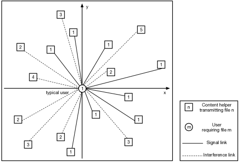
Figure 1: Spatial distribution of a content delivery network adapting CAMAC (see Section III).

The channel model is described as follows. All channels are assumed to be narrow-band and characterized by path loss and Rayleigh fading. Consider an arbitrary time slot. The signal transmitted by a transmitter at the location $X$, denoted as $Q_{X}$, is received by the typical receiver as $H_{X}\left|X\right|^{-\frac{\alpha}{2}}Q_{X}$, where $\left|X\right|$ measures the Euclidean propagation distance, $\alpha$ denotes the fixed path-loss exponent, and the fading coefficient $H_{X}$ is a ${\cal{CN}}(0,1)$ r.v. All fading coefficients are i.i.d. Consider an interference limited network where noise is negligible. Then the total received signal at the typical user can be written as:

$$Y_{0}=\sum_{n=1}^{N}\sum_{X\in\Phi_{n}}{H_{X}}\left|X\right|^{-\frac{\alpha}{2}}Q_{X}.$$ (4)

The signal is decomposed into data signal and interference in the next section based on the CAMAC algorithm. Let $\mathsf{SIR}$ denotes the resultant SIR for the typical user. Conditioned on $D_{0}=\mathcal{F}_{k}$, the conditional content-delivery probability is denoted as $P_{d}(\mathcal{F}_{k})$ and written as $P_{d}(\mathcal{F}_{k})=\Pr(\mathsf{SIR}>\theta_{k}\mid D_{0}=\mathcal{F}_{k})$, with $\theta_{k}$ is a given threshold specifying the criterion on the received signal for successful delivery of $\mathcal{F}_{k}$. Then the content-delivery probability $P_{d}=\sum_{k=1}^{N}a_{k}P_{d}(\mathcal{F}_{k})$.

III Content Adaptive Modulation and Coding

III-A CAMAC: Algorithm Design

The design of the CAMAC algorithm is simple and comprises two components: one is a mapping from files in a content database to a given number of MAC schemes and the other one is the helper architecture for adapting the MAC scheme using the mapping, which are illustrated in Fig. 2. Consider the content-MAC mapping in Fig. 2(a). The assignment of a particular MAC scheme to a given file depends on the the acceptable MAC rate given the quality requirement and the size of the content. Typically, the set of available MAC schemes is much smaller than the content database and thus each MAC scheme can be assigned to multiple files. The optimal design of the mapping depends on specific content characteristics and system parameters, which is outside the scope of the current work. Next, consider the helper architecture for implementing CAMAC as shown in Fig. 2(b). All helpers agree on an uniform content-MAC mapping which is determined by a centralized control station prior to the content-delivery phase. During content delivery, each helper uses the mapping to select a MAC scheme for modulating and coding a particular transmitted file. This spatially aligns the MAC schemes of all helpers transmitting identical content without online coordination or message exchange. As a result, as illustrated in Fig. 1, the signals transmitted by all helpers for sending identical files are combined at any receiver requesting the file as the input to the demodulator and decoder, increasing signal power and reducing interference.

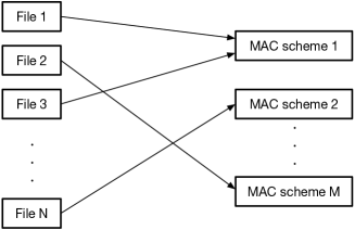
(a) Mapping between content and MAC schemes.

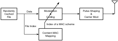
(b) Architecture of a content helper.

Figure 2: The design of content adaptive modulation and coding (CAMAC).

For tractability, two assumptions related to CAMAC are made for the network performance analysis in the sequel.

Assumption 1 (Distribution of Transmitted Signals).

The signals transmitted by helpers for sending identical files are identical. Any two transmitted signals carrying different files are independent r.v.s.

Assumption 2 (Effective Frequency-Flat Channel).

The effective multi-path channel (see Fig. 1) from helpers sending a particular file to the typical user who needs the file is frequency flat.

The assumption corresponds to the case where the path-loss exponent is relatively high such that the typical user receives only significant signals from nearby helpers. Consequently, the differentiation in the propagation delay in the signal paths is small and does not induce frequency selectivity. Otherwise, channel equalization is needed at the typical user prior to detection.

III-B CAMAC: Signal and Interference

Given the CAMAC algorithm, the expressions for signal and interference and their distributions are obtained shortly to facilitate the subsequent network-performance analysis.

Consider the case where the typical user requests $\mathcal{F}_{k}$. Given CAMAC and Assumptions 1 and 2, conditioned on $D_{0}=\mathcal{F}_{k}$, the signal can be rewritten from (4) as

$$Y_{0}(\mathcal{F}_{k})\!\!=\!\!\left(\sum_{X\in\Phi_{k}}{H_{X}}\left|X\right|^{-\frac{\alpha}{2}}\right)\!\!Q_{k}\!\!+\!\!\sum_{n\neq k}\sum_{Z\in\Phi_{n}}\!\!\left({H_{Z}}\left|Z\right|^{-\frac{\alpha}{2}}\right)\!\!Q_{n}$$

where the first and second terms correspond to (data) signal and interference, respectively. Then the signal and interference power, denoted as $S_{0}(\mathcal{F}_{k})$ and $I_{0}(\mathcal{F}_{k})$, respectively, can be written as

$$S_{0}(\mathcal{F}_{k})\!\!=\!\!\left|\sum_{X\in\Phi_{k}}\!\!{H_{X}}\left|X\right|^{-\frac{\alpha}{2}}\right|^{2}\!\!,\ I_{0}(\mathcal{F}_{k})\!\!=\!\!\sum_{n\neq k}\left|\sum_{Z\in\Phi_{n}}\!\!{H_{Z}}\left|Z\right|^{-\frac{\alpha}{2}}\right|^{2}\!\!.$$

Since $\{H_{X},H_{Z}\}$ are i.i.d. complex Gaussian r.v.s, the terms $\sum_{X\in\Phi_{k}}H_{X}\left|X\right|^{-\frac{\alpha}{2}}$ and $\sum_{Z\in\Phi_{n}}H_{Z}\left|Z\right|^{-\frac{\alpha}{2}}$ are distributed as ${\cal{CN}}(0,\sum_{X\in\Phi_{k}}\left|X\right|^{-\alpha})$ and ${\cal{CN}}(0,\sum_{Z\in\Phi_{n}}\left|Z\right|^{-\alpha})$, respectively. It follows that the signal power $S_{0}(\mathcal{F}_{k})$ follows the exponential distribution with mean $\sum_{X\in\Phi_{k}}\left|X\right|^{-\alpha}$. Moreover, the interference power can be written as $I_{0}(\mathcal{F}_{k})=\sum_{n\neq k}I_{n}$ where $I_{n}$ also follows the exponential distribution but with mean $\sum_{Z\in\Phi_{n}}\left|Z\right|^{-\alpha}$. Equivalently,

$$S_{0}(\mathcal{F}_{k})\sim h_{k}\sum_{X\in\Phi_{k}}\left|X\right|^{-\alpha},\quad I_{n}\sim h_{n}\sum_{Z\in\Phi_{n}}\left|Z\right|^{-\alpha}$$ (5)

where the operator $\sim$ denotes the equivalence in distribution, and $\{h_{k},h_{n}\}$ are i.i.d. exponential r.v.s with unit mean. Consequently, it is obvious that $S_{0}(\mathcal{F}_{k}),\{I_{n}\}$ are independent r.v.s. Using these results, the conditional content-delivery probability defined in Section II can be rewritten as

$${P}_{d}(\mathcal{F}_{k})=\Pr\left(\frac{S_{0}(\mathcal{F}_{k})}{\sum_{n\neq k}I_{n}}>\theta_{k}\right)$$ (6)

where $S_{0}(\mathcal{F}_{k})$ and $I_{n}$ are distributed as in (5).

Remark 1 (Effects of MAC Schemes).

The effect of the proposed CAMAC scheme on the analysis of content-delivery probability arises from the simple fact that two signals carrying the same file and modulated/encoded using the same MAC scheme results in the combining of two channels in the received signal [see (5)]. On the other hand, even if modulated/encoded using the same MAC scheme, two signals carrying two different files cannot lead to the said channel combining. From this aspect, the number of available MAC schemes for transmission does not affect the content-delivery probability. However, in practice, it is necessary to have multiple MAC schemes to support numerous available date rates, thereby satisfying diversified quality of service (QoS) requirements for different types of content. In the current model, the QoS requirements are reflected in the SIR thresholds $\{\theta_{k}\}$.

Remark 2 (Spatial Alignment in Practice).

In practice, the users’ requests for an identical file are generated asynchronously but the proposed CAMAC scheme requires synchronization of the transmissions by different helpers. Based on the CAMAC scheme, the helper synchronization is minimum, namely synchronization of slot boundaries, but their modulation adaptations are independent. In the scenario where a content file is small (e.g., a song or the preview of a video) and thus its transmission duration is short, forcing the said synchronization causes delay no more than half the duration, which is compensated by improved reliability in content delivery due to CAMAC. On the other hand, in the scenario where a content file is large (e.g., a movie), the proactive pushing technology (see e.g., [30]) can be deployed together with CAMAC to proactively delivery the file by different helpers to the caches of associated mobile users based on prediction of their future demands using information on past requests. In this case, the helper synchronization does not incur any additional latency as experienced by mobile users while the link reliability is enhanced by CAMAC.

IV Distribution of shot-noise ratio

One can see from (6) the content-delivery probability is closely related to a process of shot-noise ratio. For the purpose of deriving the probability, we analyze the distribution of the shot-noise ratio $R(\lambda_{1},\lambda_{2})$ defined in Section I-C. Specifically, in this section, the CCDF in (2) and the Laplace function in (3) are derived. For ease of notation, they are represented by $\bar{F}\left(x;\lambda_{1},\lambda_{2}\right)$ with $x>0$ and $\mathcal{L}_{R\left(\lambda_{1},\lambda_{2}\right)}(s)$ with any complex $s$ for which the result converges, respectively.

The derivation approach is as follows. We define a new process called a differential shot noise process as the difference between two independent shot noise process $S(\Phi_{1})$ and $S(\Phi_{2})$ as defined in (1) without fading. Mathematically, given a constant $x\in\mathbb{R}^{+}$, the differential shot noise process, denoted as $M(x;\lambda_{1},\lambda_{2})$, is defined as

$$M(x;\lambda_{1},\lambda_{2})=\sum_{X\in\Phi_{1}}|X|^{-\alpha}-x\sum_{Z\in\Phi_{2}}|Z|^{-\alpha}.$$ (7)

Then the CCDF of $R(\lambda_{1},\lambda_{2})$ is equivalent to the zero-crossing probability of $M(x;\lambda_{1},\lambda_{2})$:

$$\boxed{\bar{F}\left(x;\lambda_{1},\lambda_{2}\right)=\Pr\left(M(x)>0\right)}.$$ (8)

It is proved in Section IV-A that the distribution of $M(x;\lambda_{1},\lambda_{2})$ belongs to the class of stable distribution. Then using this factor and by exploiting the equivalence in (8), the theory of stable distribution is applied in Section IV-B to derive the desired distribution functions for the shot-noise ratio $R(\lambda_{1},\lambda_{2})$.

IV-A Distribution of a Differential Shot-Noise Process

In this section, the characteristic function for the differential shot noise process $M(x;\lambda_{1},\lambda_{2})$ is first derived. Comparing the function with that for the class of stable distribution leads to the conclusion that the process belongs to the class. The details are as follows.

As the concept of stable distribution is repeatedly used in this and next sub-sections, it is useful to provide the definition (see e.g., [31]) as follows.

Definition 1 (Stable Distribution).

A r.v. $X$ is stable in the broad sense if for any positive constants $a$ and $b$, there exist some positive $c$ and some $d\in\mathbb{R}$ such that

$$aX_{1}+bX_{2}=cX+d$$ (9)

where $X_{1}$ and $X_{2}$ are independent and identically distributed r.v.s having the same distribution as $X$. If (9) holds with $d=0$, then $X$ is strictly stable or stable in the narrow sense.

The definition implies that the distribution shape of $X$ is preserved under a linear operation with positive parameters. The characteristic function and some useful properties of the class of stable distribution are provided in Appendix -A.

It is well known that a shot noise process $S(\Phi)$ with $\alpha>2$ belongs to the class of stable distribution [28]. However, it is unknown that if the distribution of $M(x;\lambda_{1},\lambda_{2})$ is also stable. The answer is affirmative as shown in Proposition 1. To prove the result, first, the characteristic function of $M(x;\lambda_{1},\lambda_{2})$, defined as $G(t;\lambda_{1},\lambda_{2})=\mathsf{E}\left[e^{jtM(x;\lambda_{1},\lambda_{2})}\right]$ with $t\in\mathds{R}$, is derived as follows.

Lemma 1 (Characteristic Function of Differential Shot Noise).

Given $\alpha>2$, the characteristic function of the differential shot noise process $M(x;\lambda_{1},\lambda_{2})$ satisfies

$$\log G\left(t\right)=- \left(\lambda_{1}+\lambda_{2}x^{\frac{2}{\alpha}}\right)\pi\Gamma\left(1-\frac{2}{\alpha}\right)\cos\frac{\pi}{\alpha}\ \left|t\right|^{\frac{2}{\alpha}}$$

$$\times\left(1-j\mathrm{sgn}(t)\frac{\lambda_{1}-\lambda_{2}x^{\frac{2}{\alpha}}}{\lambda_{1}+\lambda_{2}x^{\frac{2}{\alpha}}}\tan\frac{\pi}{\alpha}\right)$$ (10)

where the sign function $\mathrm{sgn}(t)$ follows the definition in (39).

Proof: See Appendix -B.

Comparing the derived characteristic function with the Form-A characteristic function for stable distribution given in Lemma 7 in Appendix -A yields the following result.

Proposition 1 (Stable Distribution of Differential Shot Noise).

The process of differential shot noise, $M(x;\lambda_{1},\lambda_{2})$ belongs to the the class of stable distribution:

$$M(x;\lambda_{1},\lambda_{2})\sim S_{A}(\delta,\beta_{A},0,\mu_{A})$$ (11)

where $S_{A}$ represents the class of stable distribution in Form A as defined in Appendix -A and the parameters are given as:

$$\delta =\frac{2}{\alpha},$$

$$\beta_{A} =\frac{\lambda_{1}-\lambda_{2}x^{\frac{2}{\alpha}}}{\lambda_{1}+\lambda_{2}x^{\frac{2}{\alpha}}},$$

$$\mu_{A} =\left(\lambda_{1}+\lambda_{2}x^{\frac{2}{\alpha}}\right)\pi\Gamma\left(1-\frac{2}{\alpha}\right)\cos\frac{\pi}{\alpha}.$$ (12)

By setting $x=0$, the stable distribution of $M(0;\lambda_{1},\lambda_{2})$ reduces to a shot noise process, $S_{A}\left(\frac{2}{\alpha},1,0,\lambda_{1}\pi\Gamma\left(1-\frac{2}{\alpha}\right)\right)$ as mentioned in [28].

IV-B Distribution of a Shot-Noise Ratio

IV-B1 CCDF of a shot-noise ratio

The CCDF of a shot-noise ratio is derived by exploiting the equivalence in (8) and applying the stable-distribution properties of the differential shot-noise process $M(x;\lambda_{1},\lambda_{2})$ as discussed in the preceding sub-section.

As shown in Proposition 1, $M(x;\lambda_{1},\lambda_{2})$ has the stable distribution $S_{A}(\delta,\beta_{A},0,\mu_{A})$. To apply the properties of Form-B stable distribution with a normalized parameter $\mu_{B}=1$ in Lemma 8 in Appendix -A, the distribution of $M(x;\lambda_{1},\lambda_{2})$ can be converted into Form B by using the parametric relations in (41) and (42) in Appendix -A. Moreover, it is necessary to scaling the process $M(x;\lambda_{1},\lambda_{2})$ to have a normalized parameter $\mu_{B}=1$. Let the resultant process be denoted as $\widetilde{M}(x;\lambda_{1},\lambda_{2})$. Its distribution is derived as shown in the following lemma.

Lemma 2 (Normalized Differential Shot Noise).

The distribution of the normalize shot-noise process, $\widetilde{M}(x;\lambda_{1},\lambda_{2})$, and its relation with that of the original process $M(x;\lambda_{1},\lambda_{2})$ are given as follows:

$$\widetilde{M}(x;\lambda_{1},\lambda_{2}) \sim S_{B}\left(\frac{2}{\alpha},\beta_{B},0,1\right)$$ (13)

$$M(x;\lambda_{1},\lambda_{2}) \sim{\mu_{B}}^{\frac{\alpha}{2}}\widetilde{M}(x;\lambda_{1},\lambda_{2})$$ (14)

where $S_{B}$ denotes Form B of stable distribution as specified in Lemma 7 and the parameters are given as:

$$\beta_{B} =\frac{\alpha}{\pi}\arctan\left(\frac{\lambda_{1}-\lambda_{2}x^{\frac{2}{\alpha}}}{\lambda_{1}+\lambda_{2}x^{\frac{2}{\alpha}}}\tan\frac{\pi}{\alpha}\right),$$

$$\mu_{B} =\frac{\left(\lambda_{1}+\lambda_{2}x^{\frac{2}{\alpha}}\right)\pi\Gamma\left(1-\frac{2}{\alpha}\right)\cos\frac{\pi}{\alpha}}{\cos\frac{\pi\beta_{B}}{\alpha}}.$$ (15)

The proof is given in Appendix -C. It follows from Lemma 2 that the zero-crossing probability for $M(x;\lambda_{1},\lambda_{2})$ is equal to that for the normalized counterpart $\widetilde{M}(x;\lambda_{1},\lambda_{2})$, which is given in Lemma 8 in Appendix -A. Combining this result and the equivalence in (8) yields the CCDF for the shot-noise ratio as elaborated below.

Proposition 2 (CCDF of a Shot-Noise Ratio).

Given $\alpha>2$, the CCDF of the process of shot-noise ratio, $R(\lambda_{1},\lambda_{2})$, is given as

$$\bar{F}\left(x;\lambda_{1},\lambda_{2}\right)\!=\!\frac{\alpha}{2\pi}\arctan\left(\Big{(}\!-1\!+\frac{2}{1+\frac{\lambda_{2}}{\lambda_{1}}x^{\frac{2}{\alpha}}}\Big{)}\tan\frac{\pi}{\alpha}\right)+\frac{1}{2}.$$ (16)

Since $\arctan$ is a monotone increasing function, we can see from the above result that $\bar{F}\left(x;\lambda_{1},\lambda_{2}\right)$ monotonically decreases with the growing ratio ${\lambda_{2}}/{\lambda_{1}}$ besides $x$. In other words, the function does not depend on the exact values of the densities. For the extreme cases of $x=0$ and $x\rightarrow\infty$, the expression for $\bar{F}\left(x;\lambda_{1},\lambda_{2}\right)$ reduces to $1$ and $0$, respectively, since the shot-noise ratio is always positive and a proper r.v.

IV-B2 Laplace function of a shot-noise ratio

It is straightforward to derive the Laplace function of a shot-noise process $S(\Phi)$ in (1) by applying Campbell’s Theorem (see e.g.,[32]). This is not true for the shot-noise ratio, $R\left(\lambda_{1},\lambda_{2}\right)$, mainly due to a shot-noise process in its denominator. Specifically, applying Campbell’s Theorem reduces the two shot-noise processes in the characteristic function of $R\left(\lambda_{1},\lambda_{2}\right)$ to be only one in denominator:

$$\mathcal{L}_{R\left(\lambda_{1},\lambda_{2}\right)}(s) =\mathsf{E}\left[\prod_{X\in\Phi_{1}}e^{-\frac{s\left|X\right|^{-\alpha}}{\sum_{Z\in\Phi_{2}}\left|Z\right|^{-\alpha}}}\right]$$

$$=\mathsf{E}\Bigg{[}e^{-\lambda_{1}\pi\Gamma\left(1-\frac{2}{\alpha}\right)\left(\frac{s}{\sum_{Z\in\Phi_{2}}\left|Z\right|^{-\alpha}}\right)^{\frac{2}{\alpha}}}\Bigg{]}.$$ (17)

The current approach for deriving the function in closed form from (17) relies on applying the following expansion of the probability distribution function (PDF) of a shot-noise process [28]:

$$f_{S(\Phi)}(x)=\frac{1}{\pi x}\sum_{m=1}^{\infty} \frac{(-1)^{m+1}\Gamma(1+m\frac{2}{\alpha})\sin\pi m\frac{2}{\alpha}}{m!}$$

$$\times\left(\frac{\lambda\pi\Gamma\left(1-\frac{2}{\alpha}\right)}{x^{\frac{2}{\alpha}}}\right)^{m}.$$ (18)

The result is given in the following proposition.

Proposition 3 (Laplace Function of a Shot-Noise Ratio).

Consider a shot-noise ratio $R\left(\lambda_{1},\lambda_{2}\right)$ generated by two independent homogeneous PPPs $\Phi_{1}$ and $\Phi_{2}$ with density $\lambda_{1}$ and $\lambda_{2}$ separately. The Laplace function of $R\left(\lambda_{1},\lambda_{2}\right)$ can be written in the following series form:

$$\mathcal{L}_{R\left(\lambda_{1},\lambda_{2}\right)}\left(s\right)=\sum_{m=1}^{\infty}\frac{(-1)^{m+1}}{\Gamma(1-m\frac{2}{\alpha})}\left(\frac{\lambda_{2}}{\lambda_{1}}s^{-\frac{2}{\alpha}}\right)^{m}.$$ (19)

The proof is provided in Appendix -D.

Similar to the result in Proposition 2, the above Laplace function depends on the ratio $\lambda_{2}/\lambda_{1}$ but not the actual values of densities. The case of highly asymmetric shot-noise densities in $R(\lambda_{1},\lambda_{2})$ corresponds to $\lambda_{2}/\lambda_{1}\rightarrow 0$. For this case, the Laplace function has the following simple asymptotic form:

$$\mathcal{L}_{R\left(\lambda_{1},\lambda_{2}\right)}\left(s\right)=\frac{1}{\Gamma(1-\frac{2}{\alpha})}\frac{\lambda_{2}}{\lambda_{1}}s^{-\frac{2}{\alpha}}+O\left(\!\left(\!\frac{\lambda_{2}}{\lambda_{1}}\!\right)^{2}\right),\ \frac{\lambda_{2}}{\lambda_{1}}\rightarrow 0$$

that is a linear function of the ratio $\lambda_{2}/\lambda_{1}$.

V Content-Delivery Probability

In the preceding section, we derive the results concerning the distribution of a shot-noise ratio. In this section, they are applied to analyze the content-delivery probability.

V-A Two Forms of Content-Delivery Probability

In this sub-section, the conditional delivery probability defined in Section II is derived in two forms. Note that the expectation of the conditional probability with respect to the content-popularity distribution yields the delivery probability.

First, the conditional delivery probability is converted into the distribution function of a shot-noise ratio so as to leverage the results derived in the preceding section. One can see from (6) that the conditional probability is not exactly the distribution of the shot-noise ratio but one with a weighted sum of $(N-1)$ shot-noise processes in the denominator. However, the problem can be solved by converting the sum into a single shot-noise process by exploiting the fundamental characteristic of the shot-noise which is proved to be stable. From Definition 1, stable distribution is invariant to linear operations such as scaling and summation. Consequently, the said weighted sum, corresponding to the total interference power for the typical user, follows the same stable distribution as a single shot-noise process as shown below.

Lemma 3 (Normalized Distributions of Signal and Interference).

The signal and interference power for the typical user, as given in (5), are distributed as scaled versions of shot-noise processes with unit density:

$$S_{0}(\mathcal{F}_{k}) \sim h_{k}(a_{k}\lambda)^{\frac{\alpha}{2}}S(\bar{\Phi}_{1}),$$

$$\sum_{n\neq k}I_{n} \sim\left(\sum_{n\neq k}{h_{n}}^{\frac{2}{\alpha}}a_{n}\lambda\right)^{\frac{\alpha}{2}}S(\bar{\Phi}_{2})$$

where $S(\cdot)$ is a shot noise process without fading as defined in (1), and $\bar{\Phi}_{1}$ and $\bar{\Phi}_{2}$ are two independent homogeneous PPPs with unit density.

The proof is provided in Appendix -E.

Define a normalized shot-noise ratio, denoted as $\bar{R}$, as one generated by $\bar{\Phi}_{1}$ and $\bar{\Phi}_{2}$. It follows from Lemma 3 and (6) that the conditional delivery probability can be written in terms of $\bar{R}$ as:

$${P}_{d}(\mathcal{F}_{k})=\Pr\left({\bar{R}}\frac{h_{k}{a_{k}}^{\frac{\alpha}{2}}}{{g_{k}}^{\frac{\alpha}{2}}}>\theta_{k}\right)$$ (20)

where the set of random variables $\{g_{1},g_{2},\cdots,g_{N}\}$ are defined by $g_{k}=\sum_{n\neq k}a_{n}{h_{n}}^{\frac{2}{\alpha}}$. Using the expression, the conditional delivery probability is derived in two forms as follows.

The first form, called the expectation form, follows from substituting the CCDF of a shot-noise ratio as given in Proposition 2 into (20), and the result is obtained as follows.

Theorem 1 (Content-Delivery Probability: Expectation Form).

Given that the request by the typical user is $D_{0}=\mathcal{F}_{k}$, the conditional delivery probability is

$${P}_{d}(\mathcal{F}_{k})=\mathsf{E}_{h_{k},g_{k}} \left[\arctan\left(\Bigg{(}1-\frac{2}{1+\left(\frac{h_{k}}{\theta_{k}}\right)^{\frac{2}{\alpha}}\frac{a_{k}}{g_{k}}}\Bigg{)}\tan\frac{\pi}{\alpha}\right)\right]$$

$$\qquad\qquad\qquad\qquad\qquad\times\frac{\alpha}{2\pi}+\frac{1}{2}$$ (21)

and the content-delivery probability is ${P}_{d}=\sum_{k=1}^{N}a_{k}{P}_{d}(\mathcal{F}_{k})$.

Let the variable ${h_{k}}^{\frac{2}{\alpha}}a_{k}$ be referred to as the (fading) weighted popularity for $\mathcal{F}_{k}$. Then the ratio $\frac{{h_{k}}^{\frac{2}{\alpha}}a_{k}}{g_{k}}$, called the weighted popularity ratio, quantifies the weighted popularity of $\mathcal{F}_{k}$ with respect to that for other files. One can observe from the result in Theorem 1 that the conditional delivery probability for a particular file is a monotone increasing function of the corresponding weighted popularity ratio since the function $\arctan$ is monotone increasing. In addition, the conditional probability reduces with an increasing SIR threshold $\theta_{k}$.

For the special case of $\alpha$, the expression for the conditional content delivery probability can be simplified as follows.

Corollary 1 (Content-Delivery Probability for $\alpha=4$).

For the path-loss exponent $\alpha=4$, the conditional delivery probability can be simplified as

$${P}_{d}(\mathcal{F}_{k})=1-\frac{2}{\pi}\mathsf{E}_{h_{k},g_{k}}\left[\arctan\left(\frac{g_{k}}{a_{k}}\sqrt{\frac{\theta_{k}}{{h_{k}}}}\right)\right].$$ (22)

The proof is provided in Appendix -F.

Next, an alternative form of the conditional delivery probability can be obtained by using the Laplace function of a shot-noise ratio in the series form as given in Proposition 3. To this end, it follows from (20) and with the fact that $h_{k}$ is an exponential r.v., the conditional delivery probability can be written as

$${P}_{d}(\mathcal{F}_{k}) =\mathsf{E}_{g_{k}}\left[e^{-\theta_{k}\left(\frac{g_{k}}{a_{k}}\right)^{\frac{\alpha}{2}}{\bar{R}}^{-1}}\right]$$

$$=\mathsf{E}_{g_{k}}\left[\mathcal{L}_{{\bar{R}}^{-1}}\left(\theta_{k}\left(\frac{g_{k}}{a_{k}}\right)^{\frac{\alpha}{2}}\right)\right].$$

Substituting the result in Proposition 3 yields

$${P}_{d}(\mathcal{F}_{k})=\mathsf{E}_{g_{k}}\left[\sum_{m=1}^{\infty}\frac{(-1)^{m+1}}{\Gamma(1-m\frac{2}{\alpha})}\left(\frac{a_{k}}{{\theta_{k}}^{\frac{2}{\alpha}}g_{k}}\right)^{m}\right].$$ (23)

Since ${P}_{d}(\mathcal{F}_{k})$ converges, interchanging the order of summation and expectation in the above expression is allowed according to Fubini’s theorem, leading to the following result.

Theorem 2 (Content-Delivery Probability: Series Form).

Given that the request by the typical user is $D_{0}=\mathcal{F}_{k}$, the conditional delivery probability is

$${P}_{d}(\mathcal{F}_{k})= \sum_{m=1}^{\infty}\frac{(-1)^{m+1}}{\Gamma(1-m\frac{2}{\alpha})}\mathsf{E}\left[{g_{k}}^{-m}\right]\left(\frac{a_{k}}{{\theta_{k}}^{\frac{2}{\alpha}}}\right)^{m}$$ (24)

and the content-delivery probability is ${P}_{d}=\sum_{k=1}^{N}a_{k}{P}_{d}(\mathcal{F}_{k})$.

To relate the results in the current theorem and Theorem 1, consider the case where the SIR threshold $\theta_{k}$ is large. As a result, the conditional delivery probability in Theorem 2 can be approximated as

$${P}_{d}(\mathcal{F}_{k}) \approx\frac{a_{k}}{{\theta_{k}}^{\frac{2}{\alpha}}\Gamma(1-\frac{2}{\alpha})}\mathsf{E}\left[\frac{1}{g_{k}}\right],\qquad\theta_{k}\gg 1$$

$$\geq\frac{a_{k}}{{\theta_{k}}^{\frac{2}{\alpha}}\Gamma(1-\frac{2}{\alpha})}\cdot\frac{1}{\mathsf{E}[g_{k}]}$$ (25)

$$=\frac{a_{k}}{{\theta_{k}}^{\frac{2}{\alpha}}\Gamma(1-\frac{2}{\alpha})}\cdot\frac{1}{\sum_{n\neq k}a_{n}\mathsf{E}\left[{h_{n}}^{\frac{2}{\alpha}}\right]}$$

$$=\frac{\sin\left(\pi\frac{2}{\alpha}\right)}{\pi\frac{2}{\alpha}}{\theta_{k}}^{-\frac{2}{\alpha}}\frac{a_{k}}{1-a_{k}}$$ (26)

where (25) uses Jensen’s inequality and (26) is obtained using the formula $\Gamma(1-z)\Gamma(z)=\frac{\pi}{\sin(\pi z)}$ for non-integer $z$. It can be observed that ${P}_{d}(\mathcal{F}_{k})$ linearly increases with the growing ratio $\frac{a_{k}}{1-a_{k}}$ which is similar to the weighted popularity ratio in the remark on Theorem 1.

Remark 3 (Convergence Conditions).

The convergence of the series in (24) requires that each summation term is finite. Sufficient conditions for convergence can be derived under the following constraint:

$$\left(\frac{\mathsf{E}\left[{g_{k}}^{-m}\right]}{\Gamma(1-m\frac{2}{\alpha})}\right)^{\frac{1}{m}}\frac{a_{k}}{{\theta_{k}}^{\frac{2}{\alpha}}}<1,\qquad\forall m.$$ (27)

The details are tedious and omitted for brevity.

V-B Bounding the Content-Delivery Probability

Bounds on the conditional-delivery probabilities whose expressions are simpler than the exact ones are derived in this sub-section. The main idea is to consider the following two modified forms of the SIR in (28), denoted as $\mathsf{SIR}^{\prime}$ and $\mathsf{SIR}^{\prime\prime}$, and study their distributions:

$$\mathsf{SIR}^{\prime}(\mathcal{F}_{k}) =\frac{h_{k}\sum_{X\in\Phi_{k}}\left|X\right|^{-\alpha}}{\sum_{z\in\Phi\backslash\Phi_{k}}h_{z}\left|Z\right|^{-\alpha}},$$

$$\mathsf{SIR}^{\prime\prime}(\mathcal{F}_{k}) =\frac{h_{k}\sum_{X\in\Phi_{k}}\left|X\right|^{-\alpha}}{h_{k^{\prime}}\sum_{z\in\Phi\backslash\Phi_{k}}\left|Z\right|^{-\alpha}}.$$ (28)

They differ from $\mathsf{SIR}$ in (6) in the locations of fading coefficients. One can interpret $\mathsf{SIR}^{\prime}$ and $\mathsf{SIR}^{\prime\prime}$ as the SIRs corresponding to two artificial cases: the former without MAC alignment in the interference and the latter having uniform MAC and an identical transmitted file through out all interference. Their distributions are related to those of the actual SIR as shown below.

Lemma 4 (Bounding the SIR).

The distribution of the SIR in (6) can be bounded as

$$\Pr(\mathsf{SIR}(\mathcal{F}_{k})\geq\theta_{k}) \geq\Pr(\mathsf{SIR}^{\prime}(\mathcal{F}_{k})>\theta_{k}),$$

$$\Pr(\mathsf{SIR}(\mathcal{F}_{k})\geq\theta_{k}) \leq\Pr(\mathsf{SIR}^{\prime\prime}(\mathcal{F}_{k})\geq\theta_{k}),\quad\forall\ k$$ (29)

where $\mathsf{SIR}^{\prime}$ and $\mathsf{SIR}^{\prime\prime}$ are defined in (28).

The proof is given in Appendix -G. The expressions for the bounds in Lemma 5 can be obtained as shown below.

Lemma 5 (Modified SIRs).

The distributions of the modified SIRs in (28) are given as

$$\Pr(\mathsf{SIR}^{\prime}(\mathcal{F}_{k})>x)= \mathsf{E}_{h_{k}}\left[\arctan\left(\Big{(}1-\frac{2}{1+\eta_{k}h_{k}^{\frac{2}{\alpha}}}\Big{)}\tan\frac{\pi}{\alpha}\right)\right]$$

$$\times\frac{\alpha}{2\pi}+\frac{1}{2}$$

$$\Pr(\mathsf{SIR}^{\prime\prime}(\mathcal{F}_{k})>x)= \frac{1}{1+x^{\frac{2}{\alpha}}\left(\frac{1}{a_{k}}-1\right)}$$

where the constant $\eta_{k}=\frac{a_{k}}{(1-a_{k})\Gamma(1+\frac{2}{\alpha})x^{\frac{2}{\alpha}}}$.

The proof is provided in Appendix -H. Combining Lemmas 4 and 5 yields the following main result of this sub-section.

Theorem 3 (Bounding Content-Delivery Probability).

Using the result from Lemma 4, conditional delivery probability is bounded by

$${P}_{d}(\mathcal{F}_{k}) \geq\frac{1}{2}+\frac{\alpha}{2\pi}\mathsf{E}_{h_{k}}\left[\arctan\left(\Big{(}1-\frac{2}{1+\eta_{k}h_{k}^{\frac{2}{\alpha}}}\Big{)}\tan\frac{\pi}{\alpha}\right)\right],$$

$${P}_{d}(\mathcal{F}_{k}) \leq\frac{1}{1+\theta_{k}^{\frac{2}{\alpha}}\left(\frac{1}{a_{k}}-1\right)}$$ (30)

where the constant $\eta_{k}=\frac{a_{k}}{(1-a_{k})\Gamma(1+\frac{2}{\alpha}){\theta_{k}}^{\frac{2}{\alpha}}}$.

Remark 4 (Skewed Popularity Distribution).

For a sanity check, one can see that for a singularly popular file with $a_{k}\rightarrow 1$, both upper and lower bounds on the conditional delivery probability grow with $a_{k}$ and converge to $1$. Correspondingly, for a highly skewed popularity distribution, CAMAC effectively turns the network into one mostly broadcasting a single popular file, for which interference is negligible.

Remark 5 (Effect of Path-Loss Exponent).

In radio access networks without multi-cell cooperation, increasing the path-loss exponent reduces the number of significant interferers and thereby improving link reliability measured by e.g., outage probability (see e.g., [21]). Consequently, the path-loss exponent has a significant effect on network performance. In contrast, for the current content-delivery network with CAMAC, there exists multiple serving helpers and interferers for each user. Increasing the path-loss exponent reduces simultaneously the numbers of helpers and interferers. As the result, the effect of path-loss exponent on network performance is not significant. As an example, given $\theta=2$, the relevant factor $\theta^{\frac{2}{\alpha}}$ in the upper bound on the content-delivery probability in (3) is 1.59 for $\alpha=3$ and a similar value of 1.41 for $\alpha=4$. The fact is confirmed by simulation in the sequel.

Last, following Corollary 2, the bounds in Theorem 3 can be further simplified for the special case of $\alpha=4$ as follows.

Corollary 2 (Bounding Content-Delivery Probability for $\alpha=4$).

For the path-loss exponent $\alpha=4$, the conditional delivery probability can be bounded as follows.

• Upper bound:

  $${P}_{d}(\mathcal{F}_{k})\leq\frac{1}{1+\sqrt{\theta_{k}}\left(\frac{1}{a_{k}}-1\right)}.$$ (31)

• Lower bound A:

  $${P}_{d}(\mathcal{F}_{k})\geq\frac{1}{\sqrt{\pi}}e^{\zeta_{k}}\Gamma\left(\frac{1}{2},\zeta_{k}\right)$$

  where the constant $\zeta_{k}=\frac{\pi\theta_{k}}{4}\left(\frac{1-a_{k}}{a_{k}}\right)^{2}$.

• Lower bound B:

  $${P}_{d}(\mathcal{F}_{k})\geq 1-\frac{2}{\pi}\arctan\left(\frac{\pi\sqrt{\theta_{k}}}{2}\Big{(}\frac{1}{a_{k}}-1\Big{)}\right).$$

The proof is provided in Appendix -I.

VI Spatial Alignment Gain

In this section, we attempt to quantify the network-performance gain of CAMAC with respect to the conventional case without using the algorithm. The (MAC) spatial alignment gain, denoted as $G_{\text{align}}$, is defined as the ratio of content-delivery probabilities between the current and the mentioned conventional case.

Consider the case with CAMAC. Simulation results (see Fig. 3) shows that the upper bound on the conditional delivery probability in Theorem 3 is sufficiently tight. Thus, we approximate the probability by the bound so as to simplify the analysis:

$$P_{d}(\mathcal{F}_{k})\approx\frac{1}{1+\theta_{k}^{\frac{2}{\alpha}}\left(\frac{1}{a_{k}}-1\right)}.$$ (32)

Next, for the conventional case without CAMAC, the conditional delivery probability, denoted as $\tilde{P}_{d}(\mathcal{F}_{k})$, is given as

$$\tilde{P}_{d}(\mathcal{F}_{k})=\Pr\left(\frac{hr_{k}^{-\alpha}}{\sum_{X\in\Phi\backslash\{T_{k}\}}h_{X}\left|X\right|^{-\alpha}}>\theta_{k}\right)$$ (33)

where $r_{k}$ is the distance between the typical user to the nearest helper $T_{k}$ having $\mathcal{F}_{k}$. The procedure for deriving a closed-form expression for the above $\tilde{P}_{d}(\mathcal{F}_{k})$ is standard in the literature of stochastic geometry, involving essentially deriving the Laplace function of a shot-noise process using Campbell’s Theorem [27]. It is straightforward to modify the existing results e.g., [17, Lemma 3] to obtain the following lemma.

Lemma 6 (Content-Delivery Probability without CAMAC).

For the conventional case without CAMAC, the conditional content-delivery probability is given as

$$\tilde{P}_{d}(\mathcal{F}_{k})=\frac{1}{1+\mu\left(\theta_{k},\alpha\right)+\theta_{k}^{\frac{2}{\alpha}}\frac{2\pi}{\alpha}\csc\left(\frac{2\pi}{\alpha}\right)\left(\frac{1}{a_{k}}-1\right)}$$ (34)

where the function $\mu$ is defined as

$$\mu\left(\theta_{k},\alpha\right)=\int_{1}^{\infty}\frac{1}{1+\theta_{k}^{-1}x^{\frac{\alpha}{2}}}dx.$$ (35)

Since the scaling factor $\frac{2\pi}{\alpha}\csc\left(\frac{2\pi}{\alpha}\right)\geq 1$, it follows from the above result that

$$\tilde{P}_{d}(\mathcal{F}_{k})\leq\frac{1}{1+\mu\left(\theta_{k},\alpha\right)+\theta_{k}^{\frac{2}{\alpha}}\left(\frac{1}{a_{k}}-1\right)}.$$ (36)

It is ready to analyze the spatial-alignment gain, $G_{\text{align}}$, defined earlier. Consider the scenario of a highly skewed popularity distribution, corresponding to $\gamma\gg 1$ and $\gamma\approx 0$, respectively. As a result, $\mathcal{F}_{1}$ is dominant with $a_{1}\approx 1$ or equally popular as others with $a_{1}\approx\frac{1}{N}$. Then the content-delivery probabilities can be approximated by the conditional probabilities for $D_{0}=\mathcal{F}_{1}$: $P_{d}\approx P_{d}(\mathcal{F}_{1})$ and $\tilde{P}_{d}\approx\tilde{P}_{d}(\mathcal{F}_{1})$. Using the results in (32) and Lemma 6, the spatial-alignment gain is approximated as

$$\boxed{G_{\text{align}}\approx 1+\frac{\mu\left(\theta_{1},\alpha\right)}{1+{\theta_{1}}^{\frac{2}{\alpha}}\left(\frac{1}{a_{1}}-1\right)}}\ .$$ (37)

One can see that the $G_{\text{align}}$ grows with the popularity measure $a_{1}$. As $a_{1}$ approaches $1$, $G_{\text{align}}$ converges to the limit of $1+\mu\left(\theta_{k},\alpha\right)$. This is the inverse of the limit of $\tilde{P}_{d}(\mathcal{F}_{k})$ while that of $P_{d}(\mathcal{F}_{k})$ is one. The implication is twofold. First, the network-performance gain due to CAMAC grows with the skewness of the popularity distribution. Second, given the highly skewed distribution, a network with CAMAC operates in the noise-limited regime while a conventional network is interference limited.

VII Simulation Results

The default simulation settings are as follows unless specified otherwise. The content helpers are Poisson distributed with density $\lambda=0.1$ and all SIR threshold are given as $\theta_{k}=5$ for simplicity. The path-loss exponent is set as $\alpha=3\ \mathrm{and}\ 4$ corresponding to the general case and special case. For the popularity distribution, we adopt the widely used Zipf distribution with the content-popularity skewness $\gamma\in[0,3]$: $a_{n}=\frac{n^{-\gamma}}{\sum_{m=1}^{N}m^{-\gamma}}$ for all $n$. Last, the benchmarking case without CAMAC has the content-delivery probability given in (34).

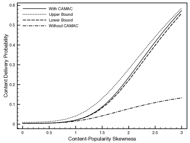
(a) Path-loss exponent $\alpha=3$

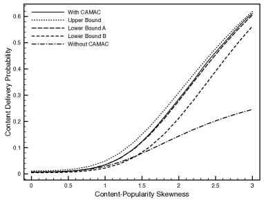
(b) Path-loss exponent $\alpha=4$

Figure 3: Comparisons of content delivery probability between the cases with and without CAMAC and evaluation of the derived bounds on the probability. The number of files is $N=50$.

Fig. 3 displays the curves of convent-delivery probability versus the content-popularity skewness for both the cases with and without CAMAC. Moreover, the derived bounds on the probability in Theorem 3 are also plotted for evaluating their tightness. One can observe that as the skewness increases, the delivery probability grows faster in the case with CAMAC than the conventional case. In particular, for skewness of $3$, the spatial-alignment gain reaches about $6$ and $3$ for $\alpha$ equal to $3$ and $4$, respectively. The smaller gain for a larger path-loss exponent is due to that more severe propagation attention suppresses interference in the conventional case and thereby helps content delivery. However, the path-loss exponent has a negligible effect when CAMAC is used, for which the network is not interference limited. Next, it is observed that the upper bound and especially the lower bound derived in Theorem 3 are tight. For the case of $\alpha=4$, there exist lower bounds A and B (see Corollary 2). The former is observed to be tighter than the latter that, however, is also capable of tracing the variation of delivery probability. Last, it is worth mentioning that, the content-delivery probability for CAMAC can be further improved by integrating the scheme with advanced communication techniques such as multi-antenna transmissions (see e.g., [24]) and successful interference cancellation [33].

The number of files in the content-data base can affect content delivery probability as revealed in Fig. 4. The analytical results in Theorems 1 and 2 are found to be identical with the simulation results shown in Fig. 4. When the content-popularity skewness is small, different files have comparable popularity. In this case, one can observe Fig. 4 that a smaller number of files amplifies the gain of CAMAC in terms of delivery probability due to larger set of signals aligned and combined by CAMAC and the corresponding reduction on interference. Nevertheless, the differentiation in delivery probability for varying the database size diminishes as the skewness growth. For this case, the popularity is concentrated in one or a few files regardless of the database size.

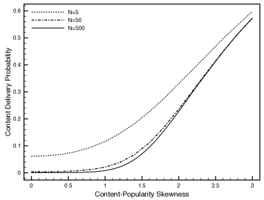
Figure 4: The effect of the number of files on the convent-delivery probability.

The approximation of the spatial alignment gain as derived in (37) is shown to be sufficiently accurate by comparing with the exact simulation results in Fig. 5. It is observed that the approximation is accurate throughout the considered range of skewness for different database sizes, even though deriving the result assumes the skewness being either high or low.

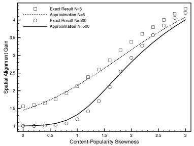
Figure 5: The spatial alignment gain and its approximation versus the content-popularity skewness. The number of files is $N=5$ or $500$.

VIII Concluding Remarks

In this work, we have proposed the idea of content adaptive modulation and coding (CAMAC) and quantify how much performance gain the idea can bring to a content delivery network. Through this work, we have shown that the spatial signal correlation in such a network can be exploited in simple ways to substantially enhance the reliability of content delivery. The performance of content-delivery networks with CAMAC can be improved by optimizing random caching strategies in the same vein as [20, 13, 17, 18, 19]. The performance gain is expected to be significant especially for the scenario of heterogeneous helpers with e.g., different storage capacities and transmission powers. The design will involve the interplay between optimization theory and the approach of shot-noise ratio developed in this work. As the current work represents an initial study of CAMAC, the implementation of the design requires further research to address various practical issues. In particular, how to cope with the frequency selectivity in the effective channels induced by CAMAC. Moreover, how to optimize the content-MAC mapping based on different quality-of-service requirements for different types of content.

In the process of network-performance analysis using a stochastic-geometry model, we have solved an open problem of finding a tractable approach for analyzing the ratio of shot-noise processes. In general, the approach and the derived results can find other applications in studying general networks with cooperative transmissions beyond the current content delivery networks with CAMAC.

-A Some Useful Properties of Stable Distribution

The characteristic function for the class of stable distribution defined in Definition 1 can be expressed in two different forms as shown below [34].

Lemma 7 (Characteristic Function for Stable Distribution [34]).

The logarithm of the characteristic function for a r.v. $X$ belonging to the class of stable distribution can be written in different forms:

• Form A

  $$\log\mathsf{E}\left[e^{jtX}\right]=\left\{\begin{aligned} jt\mu_{A}\gamma_{A}-\mu_{A}\left|t\right|^{\delta}&\Big{(}1-j\beta_{A}\ \mathrm{sgn}(t)\\ &\times\tan\frac{\pi\delta}{2}\Big{)},\ \delta\neq 1\\ jt\mu_{A}\gamma_{A}-\mu_{A}\left|t\right|&\Big{(}1+j\beta_{A}\frac{2}{\pi}\ \mathrm{sgn}(t)\\ &\times\log|t|\Big{)},\ \delta=1\end{aligned}\right.$$ (38)

  where the real parameters satisfy $\delta\in[0,2]$, $\beta_{A}\in[-1,1]$, $\gamma_{A}\in\mathds{R}$, $\mu_{A}>0$, and the sign function $\mathrm{sgn}(t)$ is defined as:

  $$\mathrm{sgn}(t)=\left\{\begin{aligned} &1,&t>0\\ &0,&t=0\\ &-1,&t<0.\end{aligned}\right.$$ (39)

• Form B

  $$\log\mathsf{E}\left[e^{jtX}\right]=\left\{\begin{aligned} jt\mu_{B}\gamma_{B}-\mu_{B}\left|t\right|^{\delta}\exp&\Big{(}-j\beta_{B}\frac{\pi}{2}\mathrm{sgn}(t)\\ &\times K(\delta)\Big{)},\ \delta\neq 1\\ jt\mu_{B}\gamma_{B}-\mu_{B}\left|t\right|\Big{(}\frac{\pi}{2}&+j\beta_{B}\mathrm{sgn}(t)\\ &\times\log|t|\Big{)},\ \delta=1\end{aligned}\right.$$ (40)

  where the parameters satisfy the same constraints as for Form A and the function $K(\delta)=\delta-1+\mathrm{sgn}(1-\delta)$.

For ease of notation, the class of stable distribution in Forms A and B are denoted as $S_{A}(\delta,\beta_{A},\gamma_{A},\mu_{A})$ and $S_{B}(\delta,\beta_{B},\gamma_{B},\mu_{B})$, respectively.

As shown in Lemma 7, a stable distribution is characterised by four parameters. The parameters $\gamma$ and $\mu$ are the location (or shift) and scale parameters, respectively. On the other hand, $\delta$ and $\beta$ essentially specify the shape of PDF. To be specific, $\delta$ is called the index of stability or characteristic exponent that is a measure of concentration; $\beta$ is called the skewness parameter that is a measure of asymmetry. By comparing Forms A and B in Lemma 7, the relations between their parameters are given as:

• For $\delta$=1,

  $$\beta_{A}=\beta_{B},\quad\gamma_{A}=\frac{2\gamma_{B}}{\pi},\quad\mu_{A}=\frac{\pi\mu_{B}}{2}.$$ (41)

• For $\delta\neq 1$,

$$\left\{\begin{aligned} \beta_{A}&=\cot\left(\frac{\pi\delta}{2}\right)\tan\left(\frac{\pi\beta_{B}K(\delta)}{2}\right),\\ \gamma_{A}&=\gamma_{B}\left(\cos\left(\frac{\pi\beta_{B}K(\delta)}{2}\right)\right)^{-1},\\ \mu_{A}&=\mu_{B}\cos\left(\frac{\pi\beta_{B}K(\delta)}{2}\right).\end{aligned}\right.$$ (42)

For several special cases, the distribution function of a stable r.v. has simple forms as shown below.

Lemma 8 (Properties of Stable Distribution [34]).

The distribution function of a stable r.v., $X$, is given for several special cases as follows.

• If $X\sim S_{B}(\delta,\beta_{B},0,1)$ and $\delta\neq 1$, then

  $$\Pr(X<0)=\frac{1}{2}\left(1-\beta_{B}\frac{K(\delta)}{\delta}\right).$$ (43)

• If $X\sim S_{B}(\delta,1,0,1)$ and $\delta<1$, then $\Pr(X<x)=0$ for all $x<0$.

• If $X\sim S_{B}(\delta,-1,0,1)$ and $\delta<1$, then $\Pr(X<x)=1$ for all $x>0$.

-B Proof of Lemma 1

The characteristic function can be written in the product form

$$\mathsf{E}\left[e^{jtM(x;\lambda_{1},\lambda_{2})}\right]=\mathsf{E} \left[e^{jt\sum_{X\in\Phi_{1}}|X|^{-\alpha}}\right]$$

$$\times\mathsf{E}\left[e^{jt\left(-x\sum_{Z\in\Phi_{2}}|Z|^{-\alpha}\right)}\right].$$ (44)

The first term in (44) is the characteristic function of a shot noise process that is well known and given as (see e.g., [27])

$$\mathsf{E}\left[e^{jt\sum_{X\in\Phi_{1}}|X|^{-\alpha}}\right] =\exp\left(j\lambda_{1}\pi t\int_{0}^{\infty}x^{-\frac{2}{\alpha}}e^{jtx}dx\right)$$

$$=e^{-\lambda_{1}\pi\Gamma\left(1-\frac{2}{\alpha}\right)\left(-jt\right)^{\frac{2}{\alpha}}}.$$ (45)

Similarly, the second term in (44) is obtained as

$$\mathsf{E}\left[e^{jt\left(-x\sum_{Z\in\Phi_{2}}|Z|^{-\alpha}\right)}\right] =e^{-\lambda_{2}\pi\Gamma\left(1-\frac{2}{\alpha}\right)\left(jtx\right)^{\frac{2}{\alpha}}}.$$ (46)

Substituting (45) and (46) into (44) leads to the following expression for the characteristic function:

$$G\left(t;\lambda_{1},\lambda_{2}\right)=e^{-\lambda_{1}\pi\Gamma\left(1-\frac{2}{\alpha}\right)\left(-jt\right)^{\frac{2}{\alpha}}}\times e^{-\lambda_{2}\pi\Gamma\left(1-\frac{2}{\alpha}\right)\left(jtx\right)^{\frac{2}{\alpha}}}.$$ (47)

Using the elementary identities $j=e^{j\frac{\pi}{2}}$ and $e^{j\frac{\pi}{\alpha}}=\cos\frac{\pi}{\alpha}+j\sin\frac{\pi}{\alpha}$, the expression can be rewritten in the desired form in the lemma statement.

-C Proof of Lemma 2

Using Proposition 1 and Lemma 7 and parametric relations in (42) in Appendix -A, the characteristic function of $M(x;\lambda_{1},\lambda_{2})$ is given as

$$\mathsf{E}\left[e^{jtM(x;\lambda_{1},\lambda_{2})}\right]=e^{-\mu_{B}\left|t\right|^{\frac{2}{\alpha}}\exp\left(-j\beta_{B}\frac{\pi}{\alpha}\mathrm{sgn}(t)\right)}.$$ (48)

Assume that the equivalence in (14) holds. Then the characteristic function of $\widetilde{M}(x;\lambda_{1},\lambda_{2})$ with the variable $t^{\prime}$ follows from the above equation by substituting $t=t^{\prime}\times{\mu_{B}}^{-\alpha/2}$. As a result,

$$\mathsf{E}\left[e^{jt^{\prime}\widetilde{M}(x;\lambda_{1},\lambda_{2})}\right]=e^{-\left|t^{\prime}\right|^{\frac{2}{\alpha}}\exp\left(-j\beta_{B}\frac{\pi}{\alpha}\mathrm{sgn}(t)\right)}.$$ (49)

Comparing the expression with the characteristic function of Form-B stable distribution in Lemma 7 in Appendix -A gives the equality in (13), confirming that $\widetilde{M}(x;\lambda_{1},\lambda_{2})$ is the normalized differential shot-noise and that the assumed result in (14) holds. This completes the proof.

-D Proof of Proposition 3

To get the result of (17), we obtain $\mathsf{E}\left[e^{-t\left(\sum_{Z\in\Phi_{2}}\left|Z\right|^{-\alpha}\right)^{-\frac{2}{\alpha}}}\right]$ first by using the series form of PDF of $S(\Phi)$ provided in (IV-B2). Accordingly,

$$\mathsf{E}\left[e^{-t\left(\sum_{Z\in\Phi_{2}}\left|Z\right|^{-\alpha}\right)^{-\frac{2}{\alpha}}}\right]$$

$$=\int_{x>0}e^{-tx^{-\frac{2}{\alpha}}}\frac{1}{\pi x}\sum_{m=1}^{\infty} \frac{(-1)^{m+1}\Gamma(1+m\frac{2}{\alpha})\sin\pi m\frac{2}{\alpha}}{m!}$$

$$\times\left(\frac{\lambda\pi\Gamma\left(1-\frac{2}{\alpha}\right)}{x^{\frac{2}{\alpha}}}\right)^{m}dx.$$ (50)

The integral in (-D) is convergent and thus according to Fubini’s theorem, we can interchange the order of integral and summation, which yields

$$\mathsf{E}\left[e^{-t\left(\sum_{Z\in\Phi_{2}}\left|Z\right|^{-\alpha}\right)^{-\frac{2}{\alpha}}}\right]$$

$$=\sum_{m=1}^{\infty}\frac{(-1)^{m+1}\Gamma(1+m\frac{2}{\alpha})\sin\pi m\frac{2}{\alpha}}{\pi m!}\left(\lambda\pi\Gamma\left(1-\frac{2}{\alpha}\right)\right)^{m}$$

$$\qquad\qquad\qquad\qquad\qquad\qquad\times\int_{0}^{\infty}e^{-tx^{-\frac{2}{\alpha}}}x^{-\frac{2}{\alpha}m-1}dx$$

$$\overset{\left(a\right)}{=}\sum_{i=1}^{\infty}\frac{\left(-1\right)^{m+1}}{\Gamma(1-m\frac{2}{\alpha})}\left(\frac{\lambda\pi\Gamma(1-\frac{2}{\alpha})}{t}\right)^{m}$$ (51)

where $(a)$ is derived from $\Gamma(1-z)\Gamma(z)=\frac{\pi}{\sin(\pi z)}$ for all non-integer $z$. Substituting $t=\lambda_{1}\pi\Gamma(1-\frac{2}{\alpha})s^{\frac{2}{\alpha}}$, $\lambda=\lambda_{2}$ and combing (17) and (-D), we can obtain the desired result.

-E Proof of Lemma 3

First, we obtain the invariance property of shot noise with respect to linear operations. Consider two independent homogeneous PPPs $\Phi_{1}$ and $\Phi_{2}$ with density $\lambda_{1}$ and $\lambda_{2}$ separately. Given two positive constants $a$ and $b$, the weighted sum of two shot-noise processes $aS(\Phi_{1})+bS(\Phi_{2})$ has a Laplace function obtained as

$$\mathsf{E}\left[e^{-s\left(a\sum_{X\in\Phi_{1}\left(\lambda_{1}\right)}\left|X\right|^{-\alpha}+b\sum_{Z\in\Phi_{2}\left(\lambda_{2}\right)}\left|Z\right|^{-\alpha}\right)}\right]$$

$$\overset{\left(a\right)}{=}\mathsf{E}\left[\prod_{X\in\Phi_{1}}e^{-sa\left|X\right|^{-\alpha}}\right]\mathsf{E}\left[\prod_{Z\in\Phi_{2}}e^{-sb\left|Z\right|^{-\alpha}}\right]$$

$$=e^{-\pi\Gamma\left(1-\frac{2}{\alpha}\right)\left(\left(\lambda_{1}a^{\frac{2}{\alpha}}+\lambda_{2}b^{\frac{2}{\alpha}}\right)^{\frac{\alpha}{2}}s\right)^{\frac{2}{\alpha}}}$$

where $(a)$ applies Campbell’s theorem [32]. It can be observed that the result is equivalent to the Laplace function of $\left(a^{\frac{2}{\alpha}}\lambda_{1}+b^{\frac{2}{\alpha}}\lambda_{2}\right)^{\frac{\alpha}{2}}S(\bar{\Phi})$ with $\bar{\Phi}$ being a PPP with unit density. Then the desired results follow from applying this property to the signal-and-interference expressions.

-F Proof of Corollary 1

When $\alpha=4$, the conditional content delivery probability in Theorem 1 is simplified as

$${P}_{d}(\mathcal{F}_{k})=\frac{1}{2}+\frac{2}{\pi}\mathsf{E}_{h_{k},g_{k}}\left[\arctan\left(\frac{1-g_{k}\sqrt{\frac{\theta_{k}}{h_{k}}}}{1+g_{k}\sqrt{\frac{\theta_{k}}{h_{k}}}}\right)\right]$$

$$=\frac{1}{2}+\frac{2}{\pi}\mathsf{E}_{h_{k},g_{k}}\left[\arctan\!\!\left(\tan\!\!\left(\frac{\pi}{4}-\arctan\left(g_{k}\sqrt{\frac{\theta_{k}}{h_{k}}}\right)\!\!\right)\!\!\right)\right]$$

which leads to the result in (22).

-G Proof of Lemma 4

Conditioned of the process $\Phi$, the delivery probability based on $\mathsf{SIR}^{\prime}$ can be expressed as

$$\Pr(\mathsf{SIR}^{\prime}>\theta_{k}\mid\Phi) =\mathsf{E}_{h_{z}}\!\!\!\left[\exp\left(-\frac{\theta_{k}\sum_{z\in\Phi\backslash\Phi_{k}}h_{z}\left|Z\right|^{-\alpha}}{\sum_{X\in\Phi_{k}}\left|X\right|^{-\alpha}}\right)\!\!\Big{|}\Phi\right]$$

$$=\!\!\!\!\prod_{{z\in\Phi\backslash\Phi_{k}}}\!\!\!\mathsf{E}_{h_{z}}\!\!\!\left[\exp\left(-\frac{\theta_{k}h_{z}\left|Z\right|^{-\alpha}}{\sum_{X\in\Phi_{k}}\left|X\right|^{-\alpha}}\right)\!\!\Big{|}\Phi\right]$$

$$=\prod_{n\neq k}\left(\prod_{{z\in\Phi_{n}}}\frac{1}{1+\frac{\theta_{k}\left|Z\right|^{-\alpha}}{\sum_{X\in\Phi_{k}}\left|X\right|^{-\alpha}}}\right)$$

$$\leq\prod_{n\neq k}\frac{1}{1+\frac{\theta_{k}\sum_{z\in\Phi_{n}}\left|Z\right|^{-\alpha}}{\sum_{X\in\Phi_{k}}\left|X\right|^{-\alpha}}}.$$ (52)

Similarly, for $\mathsf{SIR}$ and $\mathsf{SIR}^{\prime\prime}$, we have

$$\Pr(\mathsf{SIR}>\theta_{k}\mid\Phi)$$

$$=\mathsf{E}_{h_{n}}\left[\exp\left(-\frac{\theta_{k}\sum_{n\neq k}h_{n}\sum_{Z\in\Phi_{n}}\left|Z\right|^{-\alpha}}{\sum_{X\in\Phi_{k}}\left|X\right|^{-\alpha}}\right)\!\!\Big{|}\Phi\right]$$

$$=\prod_{n\neq k}\mathsf{E}_{h_{n}}\left[\exp\left(-\frac{\theta_{k}h_{n}\sum_{Z\in\Phi_{n}}\left|Z\right|^{-\alpha}}{\sum_{X\in\Phi_{k}}\left|X\right|^{-\alpha}}\right)\!\!\Big{|}\Phi\right]$$

$$=\prod_{n\neq k}\frac{1}{1+\frac{\theta_{k}\sum_{z\in\Phi_{n}}\left|Z\right|^{-\alpha}}{\sum_{X\in\Phi_{k}}\left|X\right|^{-\alpha}}}\leq\frac{1}{1+\frac{\theta_{k}\sum_{z\in\Phi\backslash\Phi_{k}}\left|Z\right|^{-\alpha}}{\sum_{X\in\Phi_{k}}\left|X\right|^{-\alpha}}},$$ (53)

$$\Pr(\mathsf{SIR}^{\prime\prime}>\theta_{k}\mid\Phi)$$

$$=\mathsf{E}_{h_{k^{\prime}}}\left[\exp\left(-\frac{\theta_{k}h_{k^{\prime}}\sum_{z\in\Phi\backslash\Phi_{k}}\left|Z\right|^{-\alpha}}{\sum_{X\in\Phi_{k}}\left|X\right|^{-\alpha}}\right)\!\!\Big{|}\Phi\right]$$

$$=\frac{1}{1+\frac{\theta_{k}\sum_{z\in\Phi\backslash\Phi_{k}}\left|Z\right|^{-\alpha}}{\sum_{X\in\Phi_{k}}\left|X\right|^{-\alpha}}}.$$ (54)

Comparing the results given in (52), (53) and (54) gives the relation in the lemma statement.

-H Proof of Lemma 5

• Proof for $\mathsf{SIR}^{\prime}$: The distribution function of $\mathsf{SIR}^{\prime}$ can be obtained as a function of shot-noise ratio without fading, as shown in the lemma below, so as to leverage relevant results.

  Lemma 9.

  The distribution function of $\mathsf{SIR}^{\prime}$ can be written in terms of shot-noise ratio without fading as follows:

  $$\Pr\!\left(\mathsf{SIR}^{\prime}\!>\!x\right)\!=\!\Pr\!\left(\!\!R\left(a_{k}\lambda,(1-a_{k})\lambda\right)\!>\!x\frac{{\Gamma\!\!\left(1+\frac{2}{\alpha}\right)}^{\frac{\alpha}{2}}}{h_{k}}\!\right)\!.$$ (55)

  Proof: According to the definitions of $\mathsf{SIR}^{\prime}$ and $R(\lambda_{1},\lambda_{2})$, leveraging exponential distribution $h_{k}$, the distribution functions in the lemma statement can be derived using Campbell’s Theorem as follows:

  $$\Pr\left(\mathsf{SIR}^{\prime}>x\right)$$

  $$=\mathsf{E}_{\Phi_{k}}\left[\exp\left(-\frac{\pi\lambda(1-a_{k})x^{\frac{2}{\alpha}}}{{\left({\sum_{X\in\Phi_{k}}\left|X\right|^{-\alpha}}\right)}^{\frac{2}{\alpha}}}\Gamma\left(1-\frac{2}{\alpha}\right)\right)\right]$$

  $$\Pr\left(R(a_{k}\lambda,(1-a_{k})\lambda)>\frac{x}{h_{k}}\right)$$

  $$=\mathsf{E}_{\Phi_{k}}\left[\exp\left(-\frac{\pi\lambda(1-a_{k})x^{\frac{2}{\alpha}}}{{\left({\sum_{X\in\Phi_{k}}\left|X\right|^{-\alpha}}\right)}^{\frac{2}{\alpha}}}\frac{2\pi}{\alpha}\csc\frac{2\pi}{\alpha}\right)\right].$$

  Comparing the right-hand sides of the above two equations reveals that they differ only in the scaling factor of $x$, which yields the desired result.  $\Box$

Combining the results in Lemma 9 and Proposition 2, we can obtain the desired result.

Proof for $\mathsf{SIR}^{\prime\prime}$: By using the Laplace function of $R(\lambda_{1},\lambda_{2})$ given in Proposition 3,

$$\Pr\left(\mathsf{SIR}^{\prime\prime}>x\right)$$

$$=\mathsf{E}\left[\mathcal{L}_{R\left(1-a_{k},a_{k}\right)}\left(xh_{k}^{\prime}\right)\right]$$

$$=\sum_{m=1}^{\infty}\frac{(-1)^{m+1}}{\Gamma(1-m\frac{2}{\alpha})}\left(\frac{a_{k}}{1-a_{k}}x^{-\frac{2}{\alpha}}\right)^{m}\mathsf{E}\left[{h_{k}^{\prime}}^{-\frac{2}{\alpha}m}\right]$$

$$\overset{\left(a\right)}{=}\sum_{m=1}^{\infty}\frac{(-1)^{m+1}}{\Gamma(1-m\frac{2}{\alpha})}\left(\frac{a_{k}}{1-a_{k}}x^{-\frac{2}{\alpha}}\right)^{m}\Gamma\left(1-m\frac{2}{\alpha}\right)$$

$$\overset{\left(b\right)}{=}\frac{1}{1+x^{\frac{2}{\alpha}}\left(\frac{1}{a_{k}}-1\right)}$$

where $(a)$ follows from $\Gamma(z)=\int_{0}^{\infty}x^{z-1}e^{-x}dx$ for all complex numbers $z$ except the non-positive integers and $(b)$ holds since the summation is a geometric series with $\frac{a_{k}}{1-a_{k}}x^{-\frac{2}{\alpha}}<1$. Similar derivation holds for $\frac{a_{k}}{1-a_{k}}x^{-\frac{2}{\alpha}}>1$ since $\Pr\left(\mathsf{SIR}^{\prime\prime}>\theta_{k}\right)=1-\mathsf{E}\left[\mathcal{L}_{R\left(a_{k},1-a_{k}\right)}\left(\frac{h_{k}}{x}\right)\right]$, yielding the same result as for the other case. This completes the proof.

-I Proof of Corollary 2

• Upper Bound: Based on the inequality in Lemma 4 and given $\alpha=4$, replacing $\mathsf{SIR}$ with $\mathsf{SIR}^{\prime\prime}$ yields

  $${P}_{d}(\mathcal{F}_{k}) \leq\Pr\left(\frac{h_{k}}{h_{k}^{\prime}\left(\frac{1-a_{k}}{a_{k}}\right)^{2}}\bar{R}>\theta_{k}\right)$$

  $$=\mathsf{E}\Big{[}e^{-h_{k}^{\prime}\theta_{k}\left(\frac{1-a_{k}}{a_{k}}\right)^{2}{\bar{R}}^{-1}}\Big{]}$$

  $$=\mathsf{E}\Bigg{[}\frac{1}{1+\theta_{k}\left(\frac{1-a_{k}}{a_{k}}\right)^{2}{\bar{R}}^{-1}}\Bigg{]}.$$

  For ease of notation, define $v=\theta_{k}\left(\frac{1-a_{k}}{a_{k}}\right)^{2}$. Since the expectation in the last expression can be derived using the CCDF of ${\bar{R}}^{-1}$, applying the result in Proposition 2 gives

  $${P}_{d}(\mathcal{F}_{k})\!\! \leq 1\!\!-\!\!\int_{0}^{\infty}\!\!\!\frac{v}{\left(1+vx\right)^{2}}\left[\frac{1}{2}\!\!+\!\!\frac{2}{\pi}\arctan\!\!\left(\frac{1-\sqrt{x}}{1+\sqrt{x}}\right)\!\!\right]\!\!dx$$

  $$=1-\int_{0}^{\infty}\frac{v}{\left(1+vx\right)^{2}}\left(1-\frac{2}{\pi}\arctan\sqrt{x}\right)\!\!dx$$

  $$\overset{\left(a\right)}{=}\frac{4}{\pi v}\int_{0}^{\infty}\frac{y}{\left(\frac{1}{v}+y^{2}\right)^{2}}\arctan{y}dy$$

  $$\overset{\left(b\right)}{=}\frac{1}{1+\sqrt{v}}=\frac{1}{1+\sqrt{\theta_{k}}\left(\frac{1}{a_{k}}-1\right)}$$

  where $(a)$ is by substituting $\sqrt{x}\rightarrow y$ and $(b)$ is obtained using the the following formula in [35, BI (252)(12)a]

  $$\int_{0}^{\infty}\frac{x\arctan qx}{\left(p^{2}+x^{2}\right)^{2}}dx=\frac{\pi q}{4p(1+pq)}.$$

• Lower Bound A: For ease of notation, define $\zeta_{k}=\frac{\pi\theta_{k}}{4}\left(\frac{1-a_{k}}{a_{k}}\right)^{2}$. Again, based on the inequality in Lemma 4 and given $\alpha=4$, replacing $\mathsf{SIR}$ with $\mathsf{SIR}^{\prime}$ leads to

  $${P}_{d}(\mathcal{F}_{k}) \geq 1-\frac{2}{\pi}\mathsf{E}_{h_{k}}\left[\arctan\left(\sqrt{\frac{\zeta_{k}}{h_{k}}}\right)\right]$$

  $$=1-\frac{2}{\pi}\int_{0}^{\infty}\arctan\left(\sqrt{\zeta_{k}}x^{-\frac{1}{2}}\right)e^{-x}dx$$

  $$\overset{\left(a\right)}{=}\!\!1-\frac{2}{\pi}\left(\!\!-\frac{\sqrt{\zeta_{k}}}{2}\int_{0}^{\infty}\!\!\frac{x^{-\frac{3}{2}}}{1+\zeta_{k}x^{-1}}e^{-x}dx+\frac{\pi}{2}\!\right)$$

  $$=\frac{\sqrt{\zeta_{k}}}{\pi}\int_{0}^{\infty}\frac{x^{-\frac{1}{2}}}{x+\zeta_{k}}e^{-x}dx$$

  where $(a)$ applies integration by parts. Using the following formula in [35, EH II 137(3)] yields the desired result from last expression

  $$\int_{0}^{\infty}\frac{x^{v-1}e^{-\mu x}}{x+\beta}dx=\beta^{v-1}e^{\beta\mu}\Gamma\left(v\right)\Gamma\left(1-v,\beta\mu\right).$$

• Lower Bound B: Using the fact that $\arctan$ is a concave function for $x>0$ and applying Jensen’s inequality, the delivery probability in (22) is bounded as

  $${P}_{d}(\mathcal{F}_{k}) \geq 1-\frac{2}{\pi}\arctan\left(\mathsf{E}\left[\frac{\sqrt{\theta_{k}}\sum_{n\neq k}a_{n}\sqrt{h_{n}}}{a_{k}\sqrt{h_{k}}}\right]\right)$$

  $$\overset{\left(a\right)}{=}1-\frac{2}{\pi}\arctan\left(\frac{\pi\sqrt{\theta_{k}}}{2}\frac{1-a_{k}}{a_{k}}\right)$$ (56)

  where $(a)$ is obtained by using the fact that $h_{k}$ and $h_{n}$ are independent and leveraging the following equalities:

  $$\int_{x>0}x^{1/2}e^{-x}dx=\sqrt{\pi}/2,\quad\int_{x>0}x^{-1/2}e^{-x}dx=\sqrt{\pi}.$$

Dongzhu Liu (S’17) received the B.Eng. from the University of Electronic Science and Technology of China (UESTC) in 2015. Since Sep. 2015, she has been a PhD student in the Dept. of Electrical and Electronic Engineering (EEE) at The University of Hong Kong. Her research interests focus on the analysis and design of wireless networks using stochastic geometry.

Kaibin Huang (M’08-SM’13) received the B.Eng. (first-class hons.) and the M.Eng. from the National University of Singapore, respectively, and the Ph.D. degree from The University of Texas at Austin (UT Austin), all in electrical engineering. Since Jan. 2014, he has been an assistant professor in the Dept. of Electrical and Electronic Engineering (EEE) at The University of Hong Kong. He used to be a faculty member in the Dept. of EEE at Yonsei University in S. Korea and currently with the department as an adjunct professor. His research interests focus on the analysis and design of wireless networks using stochastic geometry and multi-antenna techniques. He frequently serves on the technical program committees of major IEEE conferences in wireless communications. He has been the technical chair/co-chair for the IEEE CTW 2013, the Wireless Communications Symposium of IEEE GLOBECOM 2017, the Comm. Theory Symp. of IEEE GLOBECOM 2014, and the Adv. Topics in Wireless Comm. Symp. of IEEE/CIC ICCC 2014 and has been the track chair/co-chair for IEEE PIMRC 2015, IEE VTC Spring 2013, Asilomar 2011 and IEEE WCNC 2011. Currently, he is an editor for IEEE Journal on Selected Areas in Communications (JSAC) series on Green Communications and Networking, IEEE Transactions on Wireless Communications, IEEE Wireless Communications Letters. He was also a guest editor for the JSAC special issues on communications powered by energy harvesting and an editor for IEEE/KICS Journal of Communication and Networks (2009-2015). He is an elected member of the SPCOM Technical Committee of the IEEE Signal Processing Society. Dr. Huang received the 2015 IEEE ComSoc Asia Pacific Outstanding Paper Award, Outstanding Teaching Award from Yonsei, Motorola Partnerships in Research Grant, the University Continuing Fellowship from UT Austin, and a Best Paper Award from IEEE GLOBECOM 2006.

References

- [1] M. A. Maddah-Ali and U. Niesen, “Fundamental limits of caching,” IEEE Trans. on Information Theory, vol. 60, no. 5, pp. 2856–2867, 2014.
- [2] A. Ghorbel, M. Kobayashi, and S. Yang, “Content delivery in erasure broadcast channels with cache and feedback,” IEEE Trans. on Information Theory, vol. 62, no. 11, pp. 6407–6422, 2016.
- [3] K. Shanmugam, N. Golrezaei, A. G. Dimakis, A. F. Molisch, and G. Caire, “Femtocaching: Wireless content delivery through distributed caching helpers,” IEEE Trans. on Information Theory, vol. 59, no. 12, pp. 8402–8413, 2013.
- [4] J. Li, Y. Chen, Z. Lin, W. Chen, B. Vucetic, and L. Hanzo, “Distributed caching for data dissemination in the downlink of heterogeneous networks,” IEEE Trans. on Comm., vol. 63, no. 10, pp. 3553–3568, 2015.
- [5] G. Paschos, E. Bastug, I. Land, G. Caire, and M. Debbah, “Wireless caching: Technical misconceptions and business barriers,” IEEE Comm. Magazine, vol. 54, no. 8, pp. 16–22, 2016.
- [6] A. J. Goldsmith and P. P. Varaiya, “Capacity of fading channels with channel side information,” IEEE Trans. on Information Theory, vol. 43, no. 6, pp. 1986–1992, 1997.
- [7] G. Caire and S. Shamai, “On the capacity of some channels with channel state information,” IEEE Trans. on Information Theory, vol. 45, no. 6, pp. 2007–2019, 1999.
- [8] B. Blaszczyszyn and A. Giovanidis, “Optimal geographic caching in cellular networks,” in Proc. of IEEE Intl. Conf. on Comm. (ICC), June 8-12 2015.
- [9] M. Haenggi, J. G. Andrews, F. Baccelli, O. Dousse, and M. Franceschetti, “Stochastic geometry and random graphs for the analysis and design of wireless networks,” IEEE Journal on Sel. Areas in Comm., vol. 27, no. 7, 2009.
- [10] S. Krishnan and H. S. Dhillon, “Effect of user mobility on the performance of device-to-device networks with distributed caching,” IEEE Wireless Comm. Lett., 2017.
- [11] M. Afshang and H. S. Dhillon, “Optimal geographic caching in finite wireless networks,” in Proc. of IEEE Intl. Workshop in Signal Processing Advances in Wireless Comm. (SPAWC), July 3-6 2016.
- [12] D. Malak and M. Al-Shalash, “Optimal caching for device-to-device content distribution in 5G networks,” in Globecom, Dec. 8-12 2014.
- [13] M. Ji, G. Caire, and A. F. Molisch, “Wireless device-to-device caching networks: Basic principles and system performance,” IEEE Journal on Selected Areas in Communications, vol. 34, no. 1, pp. 176–189, 2016.
- [14] C. Yang, Y. Yao, Z. Chen, and B. Xia, “Analysis on cache-enabled wireless heterogeneous networks,” IEEE Trans. on Wireless Comm., vol. 15, no. 1, pp. 131–145, 2016.
- [15] E. Bastug, M. Bennis, M. Kountouris, and M. Debbah, “Cache-enabled small cell networks: Modeling and tradeoffs,” EURASIP Journal on Wireless Comm. and Net., vol. 2015, no. 1, pp. 1–11, 2015.
- [16] Y. Cui, D. Jiang, and Y. Wu, “Analysis and optimization of caching and multicasting in large-scale cache-enabled wireless networks,” IEEE Trans. on Wireless Comm., vol. 15, no. 7, pp. 5101–5112, 2016.
- [17] J. Wen, K. Huang, S. Yang, and V. O. Li, “Cache-enabled heterogeneous cellular networks: Optimal tier-level content placement,” IEEE Trans. on Wireless Comm., 2017.
- [18] Z. Chen, J. Lee, T. Q. Quek, and M. Kountouris, “Cooperative caching and transmission design in cluster-centric small cell networks,” IEEE Trans. on Wireless Comm., vol. 16, no. 5, pp. 3401–3415, 2017.
- [19] W. Wen, Y. Cui, F.-C. Zheng, and S. Jin, “Random caching based cooperative transmission in heterogeneous wireless networks,” in Proc. of IEEE Intl. Conf. on Comm. (ICC), May 21-25 2017.
- [20] Y. Chen, M. Ding, J. Li, Z. Lin, G. Mao, and L. Hanzo, “Probabilistic small-cell caching: Performance analysis and optimization,” IEEE Transactions on Vehicular Technology, vol. 66, no. 5, pp. 4341–4354, 2017.
- [21] J. G. Andrews, F. Baccelli, and R. K. Ganti, “A tractable approach to coverage and rate in cellular networks,” IEEE Trans. on Comm., vol. 59, no. 11, pp. 3122–3134, 2011.
- [22] F. Baccelli, B. Blaszczyszyn, and P. Muhlethaler, “Stochastic analysis of spatial and opportunistic aloha,” IEEE Journal on Sel. Areas in Comm., vol. 27, no. 7, 2009.
- [23] G. Nigam, P. Minero, and M. Haenggi, “Coordinated multipoint joint transmission in heterogeneous networks,” IEEE Trans. on Comm., vol. 62, no. 11, pp. 4134–4146, 2014.
- [24] K. Huang and J. G. Andrews, “An analytical framework for multicell cooperation via stochastic geometry and large deviations,” IEEE Trans. on Information Theory, vol. 59, no. 4, pp. 2501–2516, 2013.
- [25] R. Tanbourgi, S. Singh, J. G. Andrews, and F. K. Jondral, “A tractable model for noncoherent joint-transmission base station cooperation,” IEEE Trans. on Wireless Comm., vol. 13, no. 9, pp. 4959–4973, 2014.
- [26] S. Guruacharya, H. Tabassum, and E. Hossain, “SINR outage evaluation in cellular networks: saddle point approximation using normal inverse Gaussian distribution,” Online: https://arxiv.org/pdf/1701.00479.pdf.
- [27] M. Haenggi, Stochastic Geometry for Wireless Networks. Cambridge University Press, 2012.
- [28] S. B. Lowen and M. C. Teich, “Power-law shot noise,” IEEE Trans. on Information Theory, vol. 36, no. 6, pp. 1302–1318, 1990.
- [29] S. N. Chiu, D. Stoyan, W. S. Kendall, and J. Mecke, Stochastic geometry and its applications. John Wiley & Sons, 2013.
- [30] S. Zhou, J. Gong, Z. Zhou, W. Chen, and Z. Niu, “Greendelivery: Proactive content caching and push with energy-harvesting-based small cells,” IEEE Communications Magazine, vol. 53, no. 4, pp. 142–149, 2015.
- [31] J. P. Nolan, Stable Distributions - Models for Heavy Tailed Data. Boston: Birkhauser, 2015.
- [32] J. F. C. Kingman, Poisson processes. Wiley Online Library, 1993.
- [33] S. P. Weber, J. G. Andrews, X. Yang, and G. De Veciana, “Transmission capacity of wireless ad hoc networks with successive interference cancellation,” IEEE Transactions on Information Theory, vol. 53, no. 8, pp. 2799–2814, 2007.
- [34] V. M. Zolotarev, One-Dimensional Stable Distributions. American Mathematical Soc., 1986.
- [35] A. Jeffrey and D. Zwillinger, Table of integrals, series, and products. Academic Press, 2007.