Point dipole and quadrupole scattering approximation to collectively responding resonator systems

Abstract

We develop a theoretical formalism for collectively responding point scatterers where the radiating electromagnetic fields from each emitter are considered in the electric dipole, magnetic dipole, and electric quadrupole approximation. The contributions of the electric quadrupole moment to electromagnetically-mediated interactions between the scatterers are derived in detail for a system where each scatterer represents a linear $RLC$ circuit resonator, representing common metamaterial resonators in radiofrequency, microwave, and optical regimes. The resulting theory includes a closed set of equations for an ensemble of discrete resonators that are radiatively coupled to each other by propagating electromagnetic fields, incorporating potentially strong interactions and recurrent scattering processes. The effective model is illustrated and tested for examples of pairs of interacting point electric dipoles, where each pair can be qualitatively replaced by a model point emitter with different multipole radiation moments.

I Introduction

Metamaterials are artificial media which, through design, exhibit functions not observed in natural materials. The constituent components of the metamaterial are resonators that are typically much smaller than the wavelength of the electromagnetic (EM) field. Each unit cell in a metamaterial array is formed by a metamolecule whose internal structure may then consist, e.g., of a nontrivial configuration of circuit resonators. Metamolecules are closely spaced and they can also interact strongly by EM-field mediated coupling. The strong interactions result from a multiple scattering effect, whereby a resonators’ charge and current oscillations, driven by the incident field and those EM fields emitted by other resonators, produce EM fields which, in turn, drive the charge and current oscillations of other resonators. The functionalities of the metamaterial then depend on these interactions.

In principle, when the reaction of a resonator to an EM field is known, Maxwell’s equations may be solved numerically for an ensemble of resonators, taking into account the constituent structure and geometry of each resonator. In practice, however, this is computationally demanding for more than a few single elements Szabo et al. (2010), or would require simplifications, such as adapting the discrete translational symmetry of an infinite lattice Koschny et al. (2004); Pendry et al. (1999); Belov and Simovski (2005); Liu et al. (2007). An alternative approach is to provide an effective model for the individual circuit elements as point scatterers interacting with the incident and scattered EM fields. A general formalism for such an approach was developed in Ref. 6, where each metamolecule was assumed to comprise a set of pointlike circuit elements whose radiative properties were described by the lowest order electric and magnetic multipoles. The model was designed to capture the physics of each resonator, e.g., its resonance frequency and radiative emission rate, that are relevant for collective radiative coupling between large numbers of metamolecules, without the need for a detailed model of the intrinsic structure of each circuit resonator. The approach then results in a coupled set of equations for the dynamics of the resonators and EM fields. The model is not limited to circuit resonators but can also be utilized for a variety of point scatterer de Vries et al. (1998) and nanoparticle systems Mühlschlegel et al. (2005); Fromm et al. (2004); Evlyukhin et al. (2010); Wang et al. (2011).

In Ref. 6; 12; 13; 14 the general formalism of Ref. 6 was applied to derive effective dipole point scatterer approaches to model split-ring resonators; Smith et al. (2000) each arc of the resonator was described by a point emitter that possess both electric and magnetic dipoles. The resulting metamolecule of two such arcs exhibits a strong electric or magnetic dipole excitation, but notably weaker electric quadrupole excitation Fedotov et al. (2007). The model was sufficient to qualitatively describe the strong collective effects of a planar metamaterial array and its correlated subradiant excitations Jenkins et al. (2016). In related systems, it has also been used in electron-beam excitation studies of a metamaterial array Adamo et al. (2012), and the model can also incorporate additional features, such as inhomogeneous broadening Jenkins and Ruostekoski (2012c).

Many metamolecules cannot accurately be modeled by electric and magnetic dipoles alone, and treating each constituent separately may be computationally impractical. For instance, there is considerable interest in the studies of strong intrametamolecular couplings in the context of Fano transmission resonances or subradiance in the systems that are formed by combinations of several resonators Liu et al. (2009); Lovera et al. (2013); Fan et al. (2010); Hentschel et al. (2011); Frimmer et al. (2012); Dregely et al. (2011); Watson et al. (2016). Experiments on collective responses of large numbers of resonators in planar metamaterial arrays are also becoming common Fedotov et al. (2010); Papasimakis et al. (2009); Sentenac and Chaumet (2008); Lemoult et al. (2010); Adamo et al. (2012); Trepanier et al. (2013); Yang et al. (2014); Jenkins et al. (2016).

Here we extend the analysis of Ref. 6 to point emitter descriptions that includes electric quadrupole radiation. The formalism then provides an effective model of a resonator system comprising single point scatterers radiating electric dipole, quadrupole, and magnetic dipole EM fields. The EM interactions between point emitters possessing also electric quadrupole moments lead to mathematically more complicated expressions. We consider an ensemble of such effective emitters and develop a compact model for their interactions. The approach is illustrated and tested by simple examples of point electric dipoles. We compare the responses of two pairs of point electric dipoles to an effective description where each pair is replaced by a single point emitter with an electric dipole or a magnetic dipole and electric quadrupole moment.

In Sec. II, we review the theoretical model utilized to describe the interactions between resonators, and the point electric and magnetic dipole approximation of their interactions. In Sec. IV, we introduce the point emitter description with an electric quadrupole moment and describe the scattered EM fields and the interactions with other emitters. In Sec. V, we analyze in detail the point multipole interactions of different resonator systems, providing specific analytical examples. Some concluding remarks are made in Sec. VI.

II Basic formalism for discrete resonator model

Here, we introduce the basic formalism used to analyze the interaction of an EM field to closely spaced resonators. The formalism is derived in detail in Ref. 6. Here, we review how the scattered EM fields are obtained from general polarization and magnetization sources, before providing an overview of the point electric and magnetic dipole approximation of the scattered EM fields and their interactions with the resonators in Sec. III.

II.1 Radiated fields

In the general model of circuit resonator interactions with EM fields, we assume that the charge and current sources are initially driven by an incident electric displacement field ${\bf D}_{\text{in}}({\bf r},t)$, and magnetic induction ${\bf B}_{\text{in}}({\bf r},t)$ with frequency $\Omega_{0}$. The electric ${\bf E}_{\text{sc},j}({\bf r},t)$ and magnetic ${\bf H}_{\text{sc},j}({\bf r},t)$ fields scattered by resonator $j$, are a result of its oscillating polarization ${\bf P}_{j}({\bf r},t)$ and magnetization ${\bf M}_{j}({\bf r},t)$ sources. In general, the electric and magnetic fields are related to the electric displacement and magnetic induction through the auxiliary equations

$${\bf D}({\bf r},t) =\epsilon_{0}{\bf E}({\bf r},t)+{\bf P}({\bf r},t)\,\text{,}$$ (1)

$${\bf H}({\bf r},t) =\frac{1}{\mu_{0}}{\bf B}({\bf r},t)-{\bf M}({\bf r},t)\,\text{.}$$ (2)

When analyzing the EM fields and resonators, we adopt the rotating wave approximation where the dynamics is dominated by $\Omega_{0}$. In the rest of the paper, all the EM field and resonator amplitudes refer to the slowly-varying versions of the positive frequency components of the corresponding variables, where the rapid oscillations $e^{-i\Omega_{0}t}$ due to the dominant laser frequency has been factored out. The scattered EM fields are then given by Jenkins and Ruostekoski (2012a)

$${\bf E}_{\text{sc},j}({\bf r}) =\frac{k^{3}}{4\pi\epsilon_{0}}\int\text{d}^{3}r^{\prime}\,\bigg{[}{\bf G}({\bf r}-{\bf r}^{\prime})\cdotp{\bf P}_{j}({\bf r}^{\prime},t)$$

$$\quad+\frac{1}{c}{\bf G}_{\times}({\bf r}-{\bf r}^{\prime})\cdotp{\bf M}_{j}({\bf r}^{\prime},t)\bigg{]}\,\text{,}$$ (3)

$${\bf H}_{\text{sc},j}({\bf r}) =\frac{k^{3}}{4\pi}\int\text{d}^{3}r^{\prime}\,\bigg{[}{\bf G}({\bf r}-{\bf r}^{\prime})\cdotp{\bf M}_{j}({\bf r}^{\prime},t)$$

$$\quad-c{\bf G}_{\times}({\bf r}-{\bf r}^{\prime})\cdotp{\bf P}_{j}({\bf r}^{\prime},t)\bigg{]}\,\text{,}$$ (4)

where $k=\Omega/c$. Explicit expressions for the radiation kernels are Jenkins and Ruostekoski (2012a)

$${\bf G}({\bf r}) =i\bigg{[}\frac{2}{3}{\bf I}h_{0}^{(1)}(kr)+\left(\frac{\bf rr}{r^{2}}-\frac{\bf I}{3}\right)h_{2}^{(1)}(kr)\bigg{]}$$

$$\quad\quad-\frac{4\pi}{3}{\bf I}\delta(k{\bf r})\,\text{,}$$ (5)

$${\bf G}_{\times}({\bf r}) =\frac{i}{k}\nabla\times\frac{e^{ikr}}{kr}{\bf I}\,\text{.}$$ (6)

Here: the dyadic ${\bf rr}$, is the outer product of ${\bf r}$ with itself; ${\bf I}$ is the identity matrix; and $h^{(1)}_{n}(x)$ are spherical Hankel functions of the first kind, of order $n$, defined by

$$h^{(1)}_{0}(x) =-i\frac{e^{ix}}{x}\,\text{,}$$ (7)

$$h^{(1)}_{2}(x) =i\left[\frac{1}{x}+i\frac{3}{x^{2}}-\frac{3}{x^{3}}\right]e^{ix}\,\text{.}$$ (8)

The radiation kernel ${\bf G}({\bf r}-{\bf r}^{\prime})$ determines the electric (magnetic) field at ${\bf r}$, from polarization (magnetization) sources at ${\bf r}^{\prime}$ Jackson (1999). Similarly, the cross kernel ${\bf G}_{\times}({\bf r}-{\bf r}^{\prime})$, determines the electric (magnetic) field at ${\bf r}$, from magnetization (polarization) sources at ${\bf r}^{\prime}$ Jackson (1999).

Equations (3) and (4) give the total scattered EM fields as functions of the polarization and magnetization densities. In general, for sources other than point resonators, the scattered field equations are not readily solved for ${\bf P}_{j}({\bf r},t)$ and ${\bf M}_{j}({\bf r},t)$. When resonators are separated by distances less than, or of the order of a wavelength, a strongly coupled system results.

II.2 Interacting resonators

In Ref. 6, a general theory was formulated to derive a coupled set of linear equations for the EM fields and strongly coupled resonators. The state of current oscillation in each resonator $j$ is described by a single dynamic variable with units of charge $Q_{j}(t)$ and its rate of change $I_{j}(t)$, the current. The current oscillations within the $j$th resonator behave like an LC circuit with resonance frequency $\omega_{j}$,

$$\omega_{j}=\frac{1}{\sqrt{L_{j}C_{j}}}\,\text{,}$$ (9)

where $C_{j}$ and $L_{j}$ are an effective self-capacitance and self-inductance, respectively. The polarization and magnetization of a resonator can be obtained from $Q_{j}(t)$ and $I_{j}(t)$ Jenkins and Ruostekoski (2012a)

$${\bf P}_{j}({\bf r},t) =Q_{j}(t){\bf p}_{j}({\bf r})\,\text{,}$$ (10)

$${\bf M}_{j}({\bf r},t) =I_{j}(t){\bf w}_{j}({\bf r})\,\text{.}$$ (11)

The charge profile function ${\bf p}_{j}({\bf r})$ and the current profile function ${\bf w}_{j}({\bf r})$, in Eqs. (10) and (11), may be considered independent of time. The geometry of individual resonators determines the form of the respective profile functions. The polarization and magnetization densities are related to the charge and current densities of the resonators by Jenkins and Ruostekoski (2012a)

$$\rho_{j}({\bf r},t) =-\nabla\cdotp{\bf P}_{j}({\bf r},t)\,\text{,}$$ (12)

$${\bf J}_{j}({\bf r},t) =\frac{\partial}{\partial t}\big{[}{\bf P}_{j}({\bf r},t)\big{]}+\nabla\times{\bf M}_{j}({\bf r},t)\,\text{.}$$ (13)

The charge and current densities within each resonator are initially driven by the incident EM fields ${\bf D}_{\text{in}}({\bf r},t)$ and ${\bf B}_{\text{in}}({\bf r},t)$. The incident electric displacement and magnetic flux, with polarization vector ${\bf\hat{e}}_{\text{in}}$, are:

$${\bf D}_{\text{in}}({\bf r}) =D_{\text{in}}{\bf\hat{e}}_{\text{in}}e^{i{\bf k}_{\text{in}}\cdotp{\bf r}}\,\text{,}$$ (14)

$${\bf B}_{\text{in}}({\bf r}) =B_{\text{in}}\big{[}{\bf\hat{k}}_{\text{in}}\times{\bf\hat{e}}_{\text{in}}\big{]}e^{i{\bf k}_{\text{in}}\cdotp{\bf r}}\,\text{,}$$ (15)

where ${\bf\hat{k}}_{\text{in}}$ is the propagation vector of the incident EM field. The total EM fields external to resonator $j$ comprise the incident field and those fields scattered from all other resonators,

$${\bf E}_{\text{ext},j}({\bf r},t) =\frac{1}{\epsilon_{0}}{\bf D}_{\text{in}}({\bf r},t)+\sum_{i\neq j}{\bf E}_{\text{sc},i}({\bf r},t)\,\text{,}$$ (16)

$${\bf H}_{\text{ext},j}({\bf r},t) =\frac{1}{\mu_{0}}{\bf B}_{\text{in}}({\bf r},t)+\sum_{i\neq j}{\bf H}_{\text{sc},i}({\bf r},t)\,\text{.}$$ (17)

The total driving of the charge and current oscillations within the resonator is provided by the external EM fields, Eqs. (16) and (17), aligned along the direction of the source, providing a net electromagnetic force (emf) Jenkins and Ruostekoski (2012a), $\mathcal{E}_{\text{ext},j}$ and flux Jenkins and Ruostekoski (2012a), $\Phi_{\text{ext},j}$. We define the external emf and flux as Jenkins and Ruostekoski (2012a)

$$\mathcal{E}_{\text{ext},j} =\frac{1}{\sqrt{\omega_{j}L_{j}}}\int\,\text{d}^{3}r\,{\bf p}_{j}({\bf r})\cdotp{\bf E}_{\text{ext},j}({\bf r})\,\text{,}$$ (18)

$$\Phi_{\text{ext},j} =\frac{\mu_{0}}{\sqrt{\omega_{j}L_{j}}}\int\text{d}^{3}r\,{\bf w}_{j}({\bf r})\cdotp{\bf H}_{\text{ext},j}({\bf r})\,\text{.}$$ (19)

The emf and flux can be decomposed into contributions from the incident and scattered EM fields,

$$\mathcal{E}_{\text{ext},j} = \mathcal{E}_{\text{in},j}+\sum_{i\neq j}\mathcal{E}_{i,j}^{\text{sc}}\,\text{,}$$ (20)

$$\Phi_{\text{ext},j} = \Phi_{\text{in},j}+\sum_{i\neq j}\Phi_{i,j}^{\text{sc}}\,\text{.}$$ (21)

The emf and flux resulting from the driving by the incident EM field is $\mathcal{E}_{\text{in},j}$ and $\Phi_{\text{in},j}$, respectively. The driving of resonator $j$ by the scattered EM fields from resonator $i$ are the emf $\mathcal{E}_{i,j}^{\text{sc}}$ and flux $\Phi_{i,j}^{\text{sc}}$. The total driving of a resonator can be summarized by the external driving $F_{\text{ext},j}$, the sum of the incident $F_{\text{in},j}$ and scattered $F_{\text{sc},j}$ driving contributions, respectively, where Jenkins and Ruostekoski (2012a)

$$F_{\text{ext},j}=F_{\text{in},j}+F_{\text{sc},j}=F_{\text{in},j}+\sum_{i\neq j}\mathcal{C}_{ij}\,\text{,}$$ (22)

where the components

$$F_{\text{in},j} =\frac{i}{\sqrt{2}}\big{(}\mathcal{E}_{\text{in},j}+i\omega_{j}\Phi_{\text{in},j}\big{)}\,\text{,}$$ (23)

$$\big{[}\mathcal{C}\big{]}_{i\neq j} =\frac{i}{\sqrt{2}}\big{(}\mathcal{E}_{i,j}^{\text{sc}}+i\omega_{j}\Phi_{i,j}^{\text{sc}}\big{)}\,\text{.}$$ (24)

II.3 Normal modes

In order to express the coupled equations for the EM fields and resonators we introduce the slowly varying normal mode oscillator amplitudes Jenkins and Ruostekoski (2012a) $b_{j}(t)$,

$$b_{j}(t)=\frac{1}{\sqrt{2\omega_{j}}}\left[\frac{Q_{j}(t)}{\sqrt{C_{j}}}+i\frac{\phi_{j}(t)}{\sqrt{L_{j}}}\right]\,\text{.}$$ (25)

Here, the generalized coordinate for the current excitation in the resonator $j$ is the charge $Q_{j}(t)$ and $\phi_{j}(t)$ represents its conjugate momentum. In the rotating wave approximation the conjugate momentum is linearly proportional to the current Jenkins and Ruostekoski (2012a). The dynamic variable in Eq. (25) can be used to describe a general resonator with both polarization and magnetization sources.

The normal mode amplitudes $b_{j}(t)$ describe the current oscillations of the resonator. These current oscillations are subject to radiative damping due to their own emitted radiation. The driving of $b_{j}(t)$ is achieved through the external fields and resulting emf and flux. The equations of motion for $Q$ and $\phi$, $\dot{Q}=I$ and $\dot{\phi}=\mathcal{E}$, together with the scattered EM fields from each resonator and those scattered fields from other resonators result in a linear system of equations for $b_{j}(t)$. For a system which comprises $N$ resonators, these read as Jenkins and Ruostekoski (2012a)

$${\bf\dot{b}}=\mathcal{C}{\bf b}+{\bf F}_{\text{in}}\,\text{,}$$ (26)

where ${\bf b}$ is a column vector of $N$ normal oscillator amplitudes

$${\bf b}=\begin{bmatrix}b_{1}\\ b_{2}\\ \vdots\\ b_{N}\end{bmatrix}\,\text{,}$$ (27)

${\bf F}_{\text{in}}$ is a column vector formed by Eq. (23). The matrix $\mathcal{C}$ describes the interactions between the resonator’s self-generated EM fields (diagonal elements) and those scattered from different resonators [off-diagonal elements; the interaction terms in Eq. (24)] Jenkins and Ruostekoski (2012a).

As we will see (Secs. III and IV) the solutions to Eq. (24) become increasingly complicated as the complexity of the resonators increases. The diagonal elements of $\mathcal{C}$ contain the resonance frequency shift and the total decay rate $\Gamma_{j}$ Jenkins and Ruostekoski (2012a),

$$\big{[}\mathcal{C}\big{]}_{j,j}=-i(\omega_{j}-\Omega_{0})-\frac{\Gamma_{j}}{2}\,\text{.}$$ (28)

The total decay rate $\Gamma$ results from the radiative emission rate and ohmic losses. Although generally the emitters can have different resonance frequencies, here, for simplicity, we focus on the case of equal frequencies, i.e., $\omega_{j}=\omega_{0}$, for all $j$.

II.4 Collective eigenmodes

Strong multiple scattering results in collective excitation modes of the system. The collective modes of current oscillation within the system are described by the eigenvectors ${\bf v}_{n}$ of the interaction matrix $\mathcal{C}$. The corresponding eigenvalues $\xi_{n}$ have real and imaginary parts corresponding to the decay rate and resonance frequency shift of the mode,

$$\xi_{n}=-\frac{\gamma_{n}}{2}-i(\Omega_{n}-\Omega_{0})\,\text{.}$$ (29)

The number of resonators $N$, determines the number of collective modes. The collective eigenmodes can then exhibit different resonance frequencies and linewidths and line shifts Jenkins and Ruostekoski (2012a); Jenkins et al. (2016). The different modes may have superradiant or subradiant characteristics. The former occurs when the emitted radiation is enhanced by the interactions of the resonators ($\gamma_{n}>\Gamma$). The latter occurs when the radiation is suppressed and confined to the metamaterial ($\gamma_{n}<\Gamma$).

III Point electric and magnetic dipole approximation

The general model of interacting resonators summarized above and introduced formally in Ref. 6 is applicable to any type of circuit element resonators. In practice, however, some approximations to the intrinsic structure of the resonators is required. When the size of the resonator is much less than the wavelength, the resonators’ scattered EM fields are often approximated as those of point multipole sources. For split ring resonators the scattered fields are dominated by electric and magnetic dipole radiation. This motivated the formal theory of the point electric and magnetic dipole approximation, introduced in Ref. 6, which we first review here. Later, in Sec. IV, we extend the theory by deriving the point electric quadrupole approximation in the same formalism that can be used to model also more general resonator and emitter systems.

III.1 Radiating point dipoles

The electric ${\bf E}_{\text{sc},j}({\bf r})$ and magnetic ${\bf H}_{\text{sc},j}({\bf r})$ fields scattered from the $j$th resonator located at ${\bf r}^{\prime}$ due to its polarization and magnetization sources follow from Eqs. (3) and (4) with the polarization density Eq. (10) and magnetization density Eq. (11). In the electric and magnetic dipole approximation, the mode functions, ${\bf p}_{j}({\bf r})={\bf p}^{\text{d}}_{j}({\bf r})$ and ${\bf w}_{j}({\bf r})$, respectively, are defined as Jenkins and Ruostekoski (2012a)

$${\bf p}^{\text{d}}_{j}({\bf r}) =H_{j}{\bf\hat{d}}_{j}\delta({\bf r}-{\bf r}_{j})\,\text{,}$$ (30)

$${\bf w}_{j}({\bf r}) =A_{\text{M},j}{\bf\hat{m}}_{j}\delta({\bf r}-{\bf r}_{j})\,\text{.}$$ (31)

Here, the proportionality constant $H_{j}$ has units of length and the unit vector ${\bf\hat{d}}_{j}$ indicates the orientation of the electric dipole, whilst $A_{\text{M},j}$ has units of area and ${\bf\hat{m}}_{j}$ indicates the orientation of the magnetic dipole. The interaction of the resonator with its self-generated EM fields causes radiative damping to occur. The radiation rates of the electric and magnetic dipoles of the $j$th resonator are $\Gamma_{\text{E1},j}$ Jenkins and Ruostekoski (2012a) and $\Gamma_{\text{M1},j}$ Jenkins and Ruostekoski (2012a), respectively, where

$$\Gamma_{\text{E1},j} =\frac{C_{j}H_{j}^{2}\omega_{j}^{4}}{6\pi\epsilon_{0}c^{3}}\,\text{,}$$ (32)

$$\Gamma_{\text{M1},j} =\frac{\mu_{0}A_{\text{M},j}^{2}\omega_{j}^{4}}{6\pi L_{j}c^{3}}\,\text{.}$$ (33)

We account for nonradiative losses by adding the phenomenological decay rate $\Gamma_{\text{O},j}$. For simple gold or silver resonators, $\Gamma_{\text{O}}$ can be estimated by applying the Drude model of permittivity with specific material paramaters to the scattered cross section of the resonator, see e.g., Ref. 25. The total decay rate is then the sum of the radiative emission rate and ohmic losses. In the dipole approximation the total decay rate $\Gamma_{j}$ is Jenkins and Ruostekoski (2012a)

$$\Gamma_{j}=\Gamma_{\text{E1},j}+\Gamma_{\text{M1},j}+\Gamma_{\text{O},j}\,\text{.}$$ (34)

The amplitudes of the EM fields scattered by the electric and magnetic dipoles are proportional to their corresponding radiative emission rates $\Gamma_{\text{E1},j}$ and $\Gamma_{\text{M1},j}$. We write the EM fields due to the point electric and magnetic dipoles sources as Jenkins and Ruostekoski (2012a)

$${\bf E}_{\text{sc},j}({\bf r}) =b_{j}\frac{3}{2}\sqrt{\frac{k^{3}}{12\pi\epsilon_{0}}}\bigg{[}\sqrt{\Gamma_{\text{E1},j}}{\bf G}({\bf r}-{\bf r}_{j})\cdotp{\bf\hat{d}}_{j}$$

$$\quad\quad-i\sqrt{\Gamma_{\text{M1},j}}{\bf G}_{\times}({\bf r}-{\bf r}_{j})\cdotp{\bf\hat{m}}_{j}\bigg{]}\text{,}$$ (35)

$${\bf H}_{\text{sc},j}({\bf r}) =-ib_{j}\frac{3}{2}\sqrt{\frac{k^{3}}{12\pi\mu_{0}}}\bigg{[}\sqrt{\Gamma_{\text{M1},j}}{\bf G}({\bf r}-{\bf r}_{j})\cdotp{\bf\hat{m}}_{j}$$

$$\quad\quad-i\sqrt{\Gamma_{\text{E1},j}}{\bf G}_{\times}({\bf r}-{\bf r}_{j})\cdotp{\bf\hat{d}}_{j}\bigg{]}\text{.}$$ (36)

III.2 Interacting point dipoles

The incident EM field, Eqs. (14) and (15), driving the charge oscillations within a resonator resulting in the emf Jenkins and Ruostekoski (2012a) $\mathcal{E}_{\text{in},j}^{\text{E1}}$ and flux Jenkins and Ruostekoski (2012a) $\Phi_{\text{in},j}^{\text{M1}}$, follow from Eqs. (18) and (19):

$$\mathcal{E}_{\text{in},j}^{\text{E1}} =\frac{1}{\epsilon_{0}\sqrt{\omega_{j}L_{j}}}\int\text{d}^{3}r\,{\bf p}^{\text{d}}_{j}({\bf r})\cdotp{\bf D}_{\text{in}}({\bf r},t)\,\text{,}$$ (37)

$$\Phi_{\text{in},j}^{\text{M1}} =\frac{1}{\sqrt{\omega_{j}L_{j}}}\int\text{d}^{3}r\,{\bf w}_{j}({\bf r})\cdotp{\bf B}_{\text{in}}({\bf r},t)\,\text{.}$$ (38)

The scattered electric field from the $j$th resonator driving the polarization source oscillations within resonator $i\neq j$, result in the emf Jenkins and Ruostekoski (2012a) $\mathcal{E}_{i,j}^{\text{sc,E1}}$

$$\mathcal{E}_{i,j}^{\text{sc,E1}}=\sqrt{\Gamma_{\text{E1},i}\Gamma_{\text{E1},j}}\left[\mathcal{G}_{\text{E1}}\right]_{i,j}\frac{b_{j}}{\sqrt{2}}\,\text{.}$$ (39)

The matrix $\mathcal{G}_{\text{E1}}$ determines how the geometrical properties and orientations of the resonators influence the scattered electric field contributions to the emf. The diagonal elements of $\mathcal{G}_{\text{E1}}$ are zero, the off-diagonal elements, with point electric dipole sources, are

$$\big{[}\mathcal{G}_{\text{E1}}\big{]}_{i,j}=\frac{3}{2}{\bf\hat{d}}_{i}\cdotp{\bf G}({\bf r}_{i}-{\bf r}_{j})\cdotp{\bf\hat{d}}_{j}\,\text{.}$$ (40)

In a similar manner, the scattered magnetic field from the $j$th resonator driving the magnetization source oscillations within resonator $i\neq j$, results in the flux Jenkins and Ruostekoski (2012a) $\Phi_{i,j}^{\text{sc,M1}}$, where

$$\Phi_{i,j}^{\text{sc,M1}}=\frac{i}{\omega_{j}}\sqrt{\Gamma_{\text{M1},i}\Gamma_{\text{M1},j}}\left[\mathcal{G}_{\text{M1}}\right]_{i,j}\frac{b_{j}}{\sqrt{2}}\,\text{.}$$ (41)

The matrix $\mathcal{G}_{\text{M1}}$ is the magnetic counterpart of Eq. (40). The diagonal elements of $\mathcal{G}_{\text{M1}}$ are zero, the off-diagonal elements, for point magnetic dipole sources, are

$$\left[\mathcal{G}_{\text{M1}}\right]_{i,j}=\frac{3}{2}{\bf\hat{m}}_{i}\cdotp{\bf G}({\bf r}_{i}-{\bf r}_{j})\cdotp{\bf\hat{m}}_{j}\,\text{.}$$ (42)

The driving of the polarization (magnetization) sources within the $j$th resonator by the magnetic (electric) field scattered by resonator $i$ result in additional contributions to the emf and flux. We call this type of driving “cross driving”. In the dipole approximation the cross driving contributions to the emf and flux are Jenkins and Ruostekoski (2012a), $\mathcal{E}_{i,j}^{\text{sc,X1}}$ and $\Phi_{i,j}^{\text{sc,X1}}$, respectively, where

$$\mathcal{E}_{i,j}^{\text{sc,X1}} =-i\sqrt{\Gamma_{\text{E1},i}\Gamma_{\text{M1},j}}\left[\mathcal{G}_{\text{X1}}\right]_{i,j}\frac{b_{j}}{\sqrt{2}}\text{,}$$ (43)

$$\Phi_{i,j}^{\text{sc,X1}} =-\frac{1}{\omega_{j}}\sqrt{\Gamma_{\text{M1},i}\Gamma_{\text{E1},j}}\left[\mathcal{G}_{\text{X1}}\right]_{i,j}^{T}\frac{b_{j}}{\sqrt{2}}\text{.}$$ (44)

The matrix, $\mathcal{G}_{\text{X1}}$, and its transpose, $\mathcal{G}_{\text{X1}}^{T}$, are the cross driving counterparts of Eqs. (40) and (42), the off diagonal elements are

$$\left[\mathcal{G}_{\text{X1}}\right]_{i,j}=\frac{3}{2}{\bf\hat{m}}_{i}\cdotp{\bf G}_{\times}({\bf r}_{i}-{\bf r}_{j})\cdotp{\bf\hat{d}}_{j}\,\text{.}$$ (45)

In the point dipole approximation, the interactions between the resonators depend exclusively upon the orientation and relative positions of the point sources. The coupling matrix $\mathcal{C}$ is

$$\mathcal{C}=\Delta-\frac{1}{2}\Upsilon+\frac{1}{2}\Big{[}i\mathcal{C}_{\text{E1}}+i\mathcal{C}_{\text{M1}}+\mathcal{C}_{\text{X1}}+\mathcal{C}_{\text{X1}}^{T}\Big{]}\,\text{,}$$ (46)

where

$$\mathcal{C}_{\text{E1}} =\Upsilon_{\text{E1}}^{1/2}\mathcal{G}_{\text{E1}}\Upsilon_{\text{E1}}^{1/2}\,\text{,}$$ (47a)

$$\mathcal{C}_{\text{M1}} =\Upsilon_{\text{M1}}^{1/2}\mathcal{G}_{\text{M1}}\Upsilon_{\text{M1}}^{1/2}\,\text{,}$$ (47b)

$$\mathcal{C}_{\text{X1}} =\Upsilon_{\text{M1}}^{1/2}\mathcal{G}_{\text{X1}}\Upsilon_{\text{E1}}^{1/2}\,\text{.}$$ (47c)

The diagonal elements of $\mathcal{C}$ contain the detuning of the incident EM field from the resonator’s resonance frequency $\omega_{j}$ and the resonator’s total decay rate $\Gamma_{j}$. The detuning is described by the diagonal matrix $\Delta$, where Jenkins and Ruostekoski (2012a)

$$\big{[}\Delta\big{]}_{j,j}\equiv-i(\omega_{j}-\Omega_{0})\,\text{,}$$ (48)

and the decay rate by the diagonal matrix $\Upsilon$, with

$$\big{[}\Upsilon\big{]}_{j,j}=\Gamma_{\text{E1},j}+\Gamma_{\text{M1},j}+\Gamma_{\text{O},j}\,\text{.}$$ (49)

The radiative decay rates of each resonator are contained in the diagonal matrices $\Upsilon_{\text{E1}}$ and $\Upsilon_{\text{M1}}$, where,

$$\big{[}\Upsilon_{\text{E1}}\big{]}_{j,j} =\Gamma_{\text{E1},j}\,\text{,}$$ (50)

$$\big{[}\Upsilon_{\text{M1}}\big{]}_{j,j} =\Gamma_{\text{M1},j}\,\text{.}$$ (51)

IV Point electric quadrupole approximation

In Sec. II, we reviewed the general model for interacting resonators and the point electric and magnetic dipole approximation of the scattered EM fields. In this section, we extend the point dipole approximation from Sec. III, to include the point electric quadrupole contribution to the scattered EM field and its interaction with the other multipole sources.

The previously derived interaction matrix Eq. (46) between resonators that exhibit point electric and magnetic dipoles is generalized for the case of point electric quadrupoles

$$\mathcal{C}= \Delta-\frac{1}{2}\Upsilon+\frac{1}{2}\Big{[}i\mathcal{C}_{\text{E1}}+i\mathcal{C}_{\text{M1}}+\mathcal{C}_{\text{X1}}+\mathcal{C}_{\text{X1}}^{T}$$

$$+i\mathcal{C}_{\text{E2}}+i\mathcal{C}_{\text{X2e}}+i\mathcal{C}_{\text{X2e}}^{T}+\mathcal{C}_{\text{X2m}}+\mathcal{C}_{\text{X2m}}^{T}\Big{]}\,\text{.}$$ (52)

The diagonal elements of Eq. (52) contain the detuning $\Delta$ [see Eq. (48)], and the total decay rate $\Upsilon$ for the resonator

$$\big{[}\Upsilon\big{]}_{j,j}=\Gamma_{\text{E1},j}+\Gamma_{\text{M1},j}+\Gamma_{\text{E2},j}+\Gamma_{\text{O},j}\,\text{.}$$ (53)

Here, $\Gamma_{\text{E2}}$ denotes the electric quadrupole radiative emission rate. The electric and magnetic dipole emission rates are $\Gamma_{\text{E1}}$ and $\Gamma_{\text{M1}}$, respectively, see Eqs. (32) and (33). The matrices for electric and magnetic dipole interactions, $\mathcal{C}_{\text{E1}}$, $\mathcal{C}_{\text{M1}}$, and $\mathcal{C}_{\text{X1}}$ are given in Eq. (47). The additional interaction terms are similarly defined,

$$\mathcal{C}_{\text{E2}} =\Upsilon_{\text{E2}}^{1/2}\mathcal{G}_{\text{E2}}\Upsilon_{\text{E2}}^{1/2}\,\text{,}$$ (54a)

$$\mathcal{C}_{\text{X2e}} =\Upsilon_{\text{E1}}^{1/2}\mathcal{G}_{\text{X2e}}\Upsilon_{\text{E2}}^{1/2}\,\text{,}$$ (54b)

$$\mathcal{C}_{\text{X2m}} =\Upsilon_{\text{M1}}^{1/2}\mathcal{G}_{\text{X2m}}\Upsilon_{\text{E2}}^{1/2}\,\text{,}$$ (54c)

and describe: electric quadrupole–electric quadrupole; electric quadrupole–electric dipole; and electric quadrupole–magnetic dipole interactions, respectively. The transpose matrices, $\mathcal{C}_{\text{X2e}}^{T}$ and $\mathcal{C}_{\text{X2m}}^{T}$ are, respectively, the electric dipole–electric quadrupole and magnetic dipole–electric quadrupole interactions. Explicit expressions for: $\mathcal{G}_{\text{E2}}$; $\mathcal{G}_{\text{X2e}}$; and $\mathcal{G}_{\text{X2m}}$ are given in Eqs. (92); (96); and (100), respectively, and are derived in this section.

The electric dipole and magnetic dipole radiative emission rates are contained in the diagonal matrices $\Upsilon_{\text{E1}}$ and $\Upsilon_{\text{M1}}$, respectively, see Eqs. (50) and (51). The electric quadrupole radiative emission rate is contained in the equivalent diagonal matrix $\Upsilon_{\text{E2}}$, where

$$\big{[}\Upsilon_{\text{E2}}\big{]}_{j,j}=\Gamma_{\text{E2},j}\,\text{.}$$ (55)

In this section, we also derive an explicit expression for $\Gamma_{\text{E2}}$.

IV.1 Interacting point electric quadrupoles

We expand the polarization density to include the electric quadrupole term ${\bf p}^{\text{q}}_{j}({\bf r})$

$${\bf P}_{j}({\bf r},t) =Q_{j}(t){\bf p}_{j}({\bf r})\,\text{,}$$

$$=Q_{n}(t)\Big{[}{\bf p}^{\text{d}}_{j}({\bf r})+{\bf p}^{\text{q}}_{j}({\bf r})+\ldots\Big{]}\,\text{.}$$ (56)

Whilst the electric dipole term ${\bf p}^{\text{d}}_{j}({\bf r})$ is vector quantity, ${\bf p}^{\text{q}}_{j}({\bf r})$ is a tensor. The index $\alpha$ of the Cartesian component of the electric quadrupole contribution of the $j$th resonator is $p_{\alpha,j}^{\text{q}}({\bf r})$, where we define Zangwill (2013)

$$p^{\text{q}}_{\alpha,j}({\bf r})=-\sum_{\beta}A_{\alpha\beta,j}\frac{\partial}{\partial r_{\beta}}\delta({\bf r}-{\bf r}_{j})\,\text{.}$$ (57)

Here, $A_{\alpha\beta,j}$ is symmetric and traceless with dimensions of area, and the indices $\alpha,\,\beta$ refer to the Cartesian coordinates $x,y,z$ and the summation is over $\beta$. The exact form of $A_{\alpha\beta,j}$ depends on the geometry of the resonator.

The scattered electric ${\bf E}_{\text{E2},j}({\bf r})$ and magnetic ${\bf H}_{\text{E2},j}({\bf r})$ fields due to the quadrupole moment located at ${\bf r}^{\prime}$ are derived from the first terms, respectively, in Eqs. (3) and (4). Here, the spatial profile of the polarization density in Eq. (10) has Cartesian component $\alpha$ defined in Eq. (57), and we find the Cartesian component $\nu$ of ${\bf E}_{\text{E2},j}({\bf r})$ and ${\bf H}_{\text{E2,j}}({\bf r})$ are;

$$E_{\text{E2},\nu,j}({\bf r}) =\frac{Q_{j}k^{3}}{4\pi\epsilon_{0}}\sum_{\alpha}\int\text{d}^{3}r^{\prime}\,G_{\nu\alpha}({\bf r}-{\bf r}^{\prime})p^{\text{q}}_{\alpha,j}({\bf r}^{\prime})\,\text{,}$$ (58)

$$H_{\text{E2},\nu,j}({\bf r}) =-\frac{cQ_{j}k^{3}}{4\pi}\sum_{\alpha}\int\text{d}^{3}r^{\prime}\,G_{\times,\nu\alpha}({\bf r}-{\bf r}^{\prime})p^{\text{q}}_{\alpha,j}({\bf r}^{\prime})\,\text{.}$$ (59)

The radiation kernels $G_{\nu\alpha}({\bf r})$ and $G_{\times,\nu\alpha}({\bf r})$ are the tensor components ($\nu,\alpha=x,y,z$) of the radiation kernels defined in Eqs. (5) and (6), respectively.

Whilst in the electric and magnetic dipole limit the radiation kernels act directly on the moments ${\bf p}^{\text{d}}_{j}({\bf r})$ and ${\bf w}_{j}({\bf r})$, respectively, the quadrupole EM fields, Eqs. (58) and (59), are more complicated due to the derivative in $p_{\alpha,j}^{\text{q}}({\bf r})$. After integrating by parts Eqs. (58) and (59), the EM field components $\nu$ are

$$E_{\text{E2},\nu,j}({\bf r}) =\frac{Q_{j}k^{3}}{4\pi\epsilon_{0}}\sum_{\alpha,\beta}\frac{\partial}{\partial r_{\beta}}G_{\nu\alpha}({\bf r}-{\bf r}_{j})A_{\alpha\beta,j}\,\text{,}$$ (60)

$$H_{\text{E2},\nu,j}({\bf r}) =-\frac{cQ_{j}k^{3}}{4\pi}\sum_{\alpha,\beta}\frac{\partial}{\partial r_{\beta}}G_{\times,\nu\alpha}({\bf r}-{\bf r}_{j})A_{\alpha\beta,j}\,\text{.}$$ (61)

The derivatives of the radiation kernel ${\bf G}({\bf r})$ and cross kernel ${\bf G}_{\times}({\bf r})$, with respect to the Cartesian coordinate $r_{\mu=x,y,z}$ are given in App. A, see Eqs. (144) and (145).

Equations (60) and (61) are the full EM field equations evaluated at ${\bf r}$ (in Cartesian coordinates), for an oscillating electric quadrupole source located at ${\bf r}^{\prime}$. The EM fields are determined by contracting Eqs. (144) and (145), acting on the quadrupole moment $A_{\alpha\beta,j}$.

In the electric dipole approximation, it is a relatively simple exercise to expand the radiation kernel, in powers of $kr$, to obtain an expression for the electric dipole radiative decay rate. For the electric quadrupole, there is no simple expansion for Eq. (144). In order to determine an expression for the electric quadrupole (and other higher order multipoles) self-interaction strength and radiative emission rate, we find it convenient to compare the multipole radiated power Jackson (1999); Zangwill (2013) to the [rate of change of] energy of an oscillator.

The radiated power can be obtained by integrating Jackson (1999)

$$\frac{\text{d}P}{\text{d}\Omega}=\lim_{r\rightarrow\infty}r^{2}{\bf\hat{r}}\cdotp\big{[}{\bf E}({\bf r})\times{\bf H}({\bf r})\big{]}$$ (62)

over a closed spherical surface, where $\text{d}\Omega$ denotes the solid angle element and ${\bf\hat{r}}$ the vector normal to the surface. In the radiation zone, the fields ${\bf E}_{\text{rad}}({\bf r})$ and ${\bf H}_{\text{rad}}({\bf r})$ vary as $1/r$, and $|{\bf E}_{\text{rad}}({\bf r})|=c\mu_{0}|{\bf H}_{\text{rad}}({\bf r})|$. We have

$$\frac{\text{d}P}{\text{d}\Omega}=\frac{r^{2}}{c\mu_{0}}|{\bf E}_{\text{rad}}({\bf r})|^{2}\,\text{.}$$ (63)

In the limit $kr\gg 1$ we adopt the notation of Ref. 32, and define a quadrupole vector component, of the $j$th resonator ${\bf q}_{j}({\bf\hat{r}})$, where

$$[{\bf q}_{j}({\bf\hat{r}})]_{\alpha}=\sum_{\beta=1}^{3}q_{\alpha\beta,j}\hat{r}_{\beta,j}\,\text{.}$$ (64)

Here, $\alpha,\beta$ refer to the Cartesian components, ${\bf\hat{r}}$ is the unit vector in the direction of ${\bf r}$, and $q_{\alpha\beta,j}$ is the electric quadrupole moment tensor, defined as Zangwill (2013)

$$q_{\alpha\beta,j}=\frac{1}{2}\int\text{d}^{3}r\,r_{\alpha}r_{\beta}\rho_{j}({\bf r},t)\,\text{.}$$ (65)

The charge density $\rho_{j}({\bf r},t)$ in Eq. (65) is defined in Eq. (12). The electric ${\bf E}_{\text{rad,E2},j}({\bf r})$ and magnetic ${\bf H}_{\text{rad,E2},j}({\bf r})$ radiated fields from the $j$th electric quadrupole are Jackson (1999)

$${\bf E}_{\text{rad,E2},j}({\bf r}) =i\frac{k^{3}}{4\pi\epsilon_{0}}\frac{e^{ikr}}{r}{\bf\hat{r}}\times\big{[}{\bf\hat{r}}\times{\bf q}_{j}({\bf\hat{r}})\big{]}\,\text{,}$$ (66)

$${\bf H}_{\text{rad,E2},j}({\bf r}) =i\frac{ck^{3}}{4\pi}\frac{e^{ikr}}{r}{\bf\hat{r}}\times{\bf q}_{j}({\bf\hat{r}})\,\text{,}$$ (67)

where $r=|{\bf r}-{\bf r}_{j}|$. The electric quadrupole contribution to the power $P_{\text{E2}}$ is Zangwill (2013)

$$\frac{\text{d}P_{\text{E2},j}}{\text{d}\Omega}=\frac{\mu_{0}c^{3}k^{6}}{16\pi^{2}}|{\bf\hat{r}}\times{\bf q}_{j}({\bf\hat{r}})|^{2}\,\text{.}$$ (68)

The electric quadrupole radiated power $P_{\text{E2},j}$, is the integral of Eq. (68) over all angles Zangwill (2013). We find Zangwill (2013) [see App. A.1],

$$P_{\text{E2},j}=\frac{\mu_{0}c^{3}k^{6}}{20\pi}\sum_{\alpha,\beta}\Big{[}q_{\alpha\beta,j}q_{\alpha\beta,j}-\frac{1}{3}q_{\alpha\alpha,j}q_{\beta\beta,j}\Big{]}\,\text{,}$$ (69)

The quadrupole moment tensors, $q_{\alpha\beta,j}$ and $A_{\alpha\beta,j}$, and the dynamic variable $b_{j}(t)$ of the $j$th resonator are related through the charge density $\rho_{j}({\bf r},t)$. The electric quadrupole component of the charge density, from Eqs. (12) and (57) is

$$\rho({\bf r},t)=Q_{j}(t)\sum_{\alpha\beta,j}\frac{\partial}{\partial r_{\alpha}}\left[A_{\alpha\beta,j}\frac{\partial}{\partial r_{\beta}}\delta({\bf r}-{\bf r}_{j})\right]\,\text{,}$$ (70)

where the summation is over the Cartesian coordinates ($\alpha,\beta=x,y,z$). Substituting Eq. (70) into Eq. (65),

$$q_{\alpha\beta,j}=\frac{1}{2}Q_{j}(t)\int\text{d}^{3}r\,r_{\mu}r_{\nu}\frac{\partial}{\partial r_{\alpha}}\left[A_{\alpha\beta,j}\frac{\partial}{\partial r_{\beta}}\delta({\bf r}-{\bf r}_{j})\right]\,\text{.}$$ (71)

Integration of Eq. (71), by parts twice yields

$$q_{\alpha\beta,j}=\frac{1}{2}Q_{j}(t)\int\text{d}^{3}r\,\left[\frac{\partial}{\partial r_{\alpha}}\frac{\partial}{\partial r_{\beta}}r_{\mu}r_{\nu}\right]A_{\alpha\beta,j}\delta({\bf r}-{\bf r}_{j})\,\text{.}$$ (72)

The term in parenthesis in Eq. (72), simplifies considerably because the derivatives result in Kronecker $\delta$ functions,

$$\frac{\partial}{\partial r_{\alpha}}\frac{\partial}{\partial r_{\beta}}r_{\mu}r_{\nu} =\frac{\partial}{\partial r_{\alpha}}\left[\delta_{\beta\mu}r_{\nu}+\delta_{\beta\nu}r_{\mu}\right]\,\text{,}$$

$$\quad=\delta_{\alpha\nu}\delta_{\beta\mu}+\delta_{\alpha\mu}\delta_{\beta\nu}=2\,\text{.}$$ (73)

Writing the charge $Q_{j}(t)$ in terms of the dynamic variable $b_{j}(t)$ [see Eq. (25)], we finally have the relationship between $q_{\alpha\beta,j},\,b_{j}(t)$ and $A_{\alpha\beta,j}$;

$$q_{\alpha\beta,j}=\sqrt{\frac{\omega_{j}C_{j}}{2}}b_{j}(t)A_{\alpha\beta,j}\,\text{.}$$ (74)

The energy $U_{j}$ of an isolated oscillator, from its Hamiltonian, is analogous to that of an LC circuit Jenkins and Ruostekoski (2012a)

$$U_{j}(t)=\omega_{j}\left|b_{j}\right|^{2}\,\text{.}$$ (75)

The electric quadrupole radiated power $P_{\text{E2},j}$ of the oscillator, is the rate of change of Eq. (75),

$$P_{\text{E2},j}=-\frac{\text{d}U_{j}}{\text{d}t}=\omega_{j}\Gamma_{\text{E2},j}\left|b_{j}\right|^{2}\,\text{.}$$ (76)

Here, $\omega_{j}$ is the resonance frequency and $\Gamma_{\text{E2},j}$ the decay rate of the electric quadrupole. Comparing Eqs. (69) and (76), we obtain the rate at which a resonator radiates energy in the point electric quadrupole approximation as

$$\Gamma_{\text{E2},j}=\frac{C_{j}A_{\text{E},j}^{2}\omega_{j}^{6}}{20\pi\epsilon_{0}c^{5}}\,\text{,}$$ (77)

where we define

$$A_{\text{E},j}^{2}=\sum_{\alpha,\beta}\left[A_{\alpha\beta,j}A_{\alpha\beta,j}-\frac{1}{3}A_{\alpha\alpha,j}A_{\beta\beta,j}\right]\,\text{,}$$ (78)

as an effective area of the electric quadrupole. Again, the indices $\alpha,\beta$ refer to the Cartesian components of the quadrupole moment and repeated indices are summed over.

With the radiative emission rates of the electric quadrupole Eq. (77), and the electric and magnetic dipoles Eqs. (32) and (33), respectively, we can express the normal mode oscillator amplitudes Eq. (25) in terms of the contributing multipole moments

$$b_{j}(t) =\sqrt{\frac{k^{3}}{12\pi\epsilon_{0}}}\Bigg{[}Q_{j}\frac{H_{j}}{\sqrt{\Gamma_{\text{E1},j}}}+kQ_{j}\sqrt{\frac{3}{5}}\frac{A_{\text{E},j}}{\sqrt{\Gamma_{\text{E2,j}}}}$$

$$\hskip 14.22636pt+i\frac{I_{j}}{c}\frac{A_{\text{M},j}}{\sqrt{\Gamma_{\text{M1},j}}}\Bigg{]}\,\text{.}$$ (79)

The real part of Eq. (79) comprises the electric dipole and electric quadrupole contributions. The imaginary part corresponds to the magnetic dipole contribution.

In the point emitter approximation, the radiative emission rates of the magnetic dipole and the electric quadrupole both depend on their respective, effective cross sectional areas $A_{\text{M},j}$ and $A_{\text{E},j}$, see Eqs. (33) and (77), respectively. For simplicity, we assume that the magnetic dipole and electric quadrupole have the same resonance frequency $\omega_{j}$ [Eq. (9)]. Comparing Eqs. (33) and (77), we find $\Gamma_{\text{M1},j}$ and $\Gamma_{\text{E2},j}$ are of the same order of magnitude, their relative radiation emission rates are

$$\frac{\Gamma_{\text{E2},j}}{\Gamma_{\text{M1},j}}=\frac{3}{10}\frac{A_{\text{E},j}^{2}}{A_{\text{M},j}^{2}}\,\text{.}$$ (80)

In Sec. III, the amplitudes of the scattered EM fields were proportional to the electric dipole and magnetic dipole radiative emission rates. Here, the full electric quadrupole EM field amplitudes, Eqs. (60) and (61), are proportional to the electric quadrupole decay rate $\Gamma_{\text{E2},j}$. We write the scaled EM fields of the $j$th electric quadrupole source as

$$E_{\text{E2},\nu,j}({\bf r}) =b_{j}\sqrt{\frac{\wp_{0}}{\epsilon_{0}}}\sum_{\alpha,\beta}\frac{\partial}{\partial kr_{\beta}}G_{\nu\alpha}({\bf r}-{\bf r}_{j}){\hat{A}}_{\alpha\beta,j}\,\text{,}$$ (81)

$$H_{\text{E2},\nu,j}({\bf r}) =-b_{j}\sqrt{\frac{\wp_{0}}{\mu_{0}}}\sum_{\alpha,\beta}\frac{\partial}{\partial kr_{\beta}}G_{\times,\nu\alpha}({\bf r}-{\bf r}_{j}){\hat{A}}_{\alpha\beta,j}\,\text{,}$$ (82)

where the constant $\wp_{0}$ is defined as

$$\wp_{0}=\frac{5k^{3}}{8\pi}\Gamma_{\text{E2},j}\,\text{,}$$ (83)

and ${\hat{A}}_{\alpha\beta,j}$ is a tensor which defines the charge configuration of the quadrupole moment

$$\hat{A}_{\alpha\beta,j}=\frac{A_{\alpha\beta,j}}{A_{\text{E},j}}\,\text{.}$$ (84)

The $j$th electric quadrupole is also driven by the external electric fields ${\bf E}_{\text{ext},j}({\bf r})$, resulting in the induced emf

$$\mathcal{E}_{\text{ext},j}^{\text{E2}}=\frac{1}{\sqrt{\omega_{j}L_{j}}}\sum_{\nu}\int\text{d}^{3}r\,p_{\nu,j}^{\text{q}}({\bf r})E_{\text{ext},\nu,n}({\bf r})\,\text{.}$$ (85)

Here, the mode function $p_{\nu,j}^{\text{q}}({\bf r})$ is defined in Eq. (57). For point electric quadrupole sources, the $j$th electric quadrupole moment $A_{\alpha\beta,j}$ interacts with gradient of the external electric field,

$$\mathcal{E}_{\text{ext},j}^{\text{E2}}=\frac{1}{\sqrt{\omega_{j}L_{j}}}\sum_{\alpha\beta}A_{\alpha\beta,j}\bigg{[}\frac{\partial}{\partial r_{\beta}}E_{\text{ext},\alpha,j}({\bf r})\bigg{]}\,\text{.}$$ (86)

The external electric field [Eq. (16)] comprises the incident electric field and the different multipole scattered fields. These different contributions to the external electric field driving the electric quadrupole source allow us to decompose the resulting emf into different components;

$$\mathcal{E}_{\text{ext},j}^{\text{E2}}=\mathcal{E}_{\text{in},j}^{\text{E2}}+\sum_{i\neq j}\Big{[}\mathcal{E}_{i,j}^{\text{sc,X2e}}+\mathcal{E}_{i,j}^{\text{sc,X2m}}+\mathcal{E}_{i,j}^{\text{sc,E2}}+\ldots\Big{]}\,\text{.}$$ (87)

In Eq. (87), the incident EM field contribution to the emf follows from Eq. (86), with the incident displacement field Eq. (14)

$$\mathcal{E}_{\text{in},j}^{\text{E2}}=\frac{1}{\epsilon_{0}\sqrt{\omega_{j}L_{j}}}\sum_{\alpha\beta}A_{\alpha\beta,j}\bigg{[}\frac{\partial}{\partial r_{\beta}}D_{\text{in},\alpha,j}({\bf r})\bigg{]}\,\text{.}$$ (88)

The contributions $\mathcal{E}_{i,j}^{\text{sc,X2e}}$ and $\mathcal{E}_{i,j}^{\text{sc,X2m}}$ are due to the interactions of electric and magnetic dipoles, respectively, with electric quadrupoles. We discuss these contributions in detail later. Here, we provide the electric quadrupole driven contribution to the emf from two interacting electric quadrupoles, $\mathcal{E}_{i,j}^{\text{sc,E2}}$, the counterpart to the emf from two electric dipoles [see Eq. (39)]. With the definition of the emf, Eq. (85), we have

$$\mathcal{E}_{i,j}^{\text{sc,E2}}=-\frac{1}{\sqrt{\omega_{j}L_{j}}}\frac{Q_{j}k^{3}}{4\pi\epsilon_{0}}\sum_{\nu}\int\text{d}^{3}r\,\left[\sum_{\eta}A_{\nu\eta,i}\frac{\partial}{\partial r_{\eta}}\delta({\bf r}-{\bf r}_{i})\right]\left[\sum_{\alpha\beta}\frac{\partial}{\partial r_{\beta}}G_{\nu\alpha}({\bf r}-{\bf r}_{j})A_{\alpha\beta,j}\right]\,\text{.}$$ (89)

The first term in parenthesis in Eq. (89) is the mode function $p_{\nu,i}^{\text{q}}({\bf r})$ of the $i$th electric quadrupole [see Eq. (57)]. Whilst the second term in parenthesis, is the scattered electric field from the $j$th electric quadrupole, $E_{\text{E2},\nu,j}({\bf r})$ [see Eq. (60)]. Integration of Eq. (89) by parts, we have

$$\mathcal{E}_{i,j}^{\text{sc,E2}}=\frac{1}{\sqrt{\omega_{j}L_{j}}}\frac{Q_{j}k^{3}}{4\pi\epsilon_{0}}\sum_{\nu}\int\text{d}^{3}r\,A_{\nu\eta,i}\delta({\bf r}-{\bf r}_{i})\sum_{\eta\alpha\beta}\bigg{[}\frac{\partial}{\partial r_{\eta}}\frac{\partial}{\partial r_{\beta}}G_{\nu\alpha}({\bf r}_{i}-{\bf r}_{j})\bigg{]}A_{\alpha\beta,j}\,\text{.}$$ (90)

The integral in Eq. (90) is readily carried out over the $\delta$ function. The second derivatives of the radiation kernel with respect to the Cartesian coordinate $r_{\mu=x,y,z}$ are given in Eqs. (148) and (149), see App. A. The electric quadrupole moment $A_{\alpha\beta,j}$, in Eq. (90), and the decay rate $\Gamma_{\text{E2},j}$ are related through the effective area $A_{\text{E},j}$ appearing in both Eqs. (77) and (84). This allows us to write Eq. (90) more compactly as

$$\mathcal{E}_{i,j}^{\text{sc,E2}}=\sqrt{\Gamma_{\text{E2},i}\Gamma_{\text{E2},j}}\left[\mathcal{G}_{\text{E2}}\right]_{i,j}\frac{b_{j}}{\sqrt{2}}\,\text{.}$$ (91)

The matrix $\mathcal{G}_{\text{E2}}$ is the contribution to $\mathcal{C}_{\text{E2}}$ in Eq. (54a), with off diagonal components

$$\left[\mathcal{G}_{\text{E2}}\right]_{i,j}=\frac{15}{4}\sum_{\nu,\eta,\alpha,\beta}{\hat{A}}_{\nu\eta,i}\frac{\partial^{2}}{\partial kr_{\eta}\partial kr_{\beta}}G_{\nu\alpha}({\bf r}_{i}-{\bf r}_{j}){\hat{A}}_{\alpha\beta,j}\,\text{.}$$ (92)

Equation (92) is, in general, complicated, however, as we show later in Sec. V.3, for simple point quadrupole systems, Eq. (92) simplifies considerably. The coupling matrix $\mathcal{C}$ for interacting electric quadrupoles only is

$$\mathcal{C}=\Delta-\frac{1}{2}\Upsilon+\frac{i}{2}\mathcal{C}_{\text{E2}}\,\text{,}$$ (93)

where $\mathcal{C}_{\text{E2}}$ is given in Eq. (54a). The diagonal elements of $\mathcal{C}$ contain the detuning $\Delta$ and total decay rate $\Upsilon$. Equation (48) gives the detuning, the decay rates in the electric quadrupole approximation are

$$\big{[}\Upsilon\big{]}_{j,j} =\Gamma_{\text{E2},j}+\Gamma_{\text{O},j}\,\text{.}$$ (94)

IV.2 Interacting point electric and magnetic dipoles and electric quadrupoles

In Sec. IV we discussed the interactions between two point electric quadrupoles and in Sec. III between electric and magnetic dipoles. Here we introduce the cross coupling of the electric quadrupole to the electric and magnetic dipoles.

IV.2.1 Electric dipole–electric quadrupole interactions

The electric field scattered by an electric dipole is given by the first integral in Eq. (35) and by an electric quadrupole in Eq. (81). These scattered electric fields drive the charge oscillations in other resonators with electric quadrupoles and electric dipoles, giving rise to the cross driving (dipole-quadrupole) emf $\mathcal{E}_{i,j}^{\text{sc,X2e}}$, where

$$\mathcal{E}_{i,j}^{\text{sc,X2e}}= \Bigg{[}\sqrt{\Gamma_{\text{E2},i}\Gamma_{\text{E1},j}}\left[\mathcal{G}_{\text{X2e}}\right]_{i,j}$$

$$\quad+\sqrt{\Gamma_{\text{E1},i}\Gamma_{\text{E2},j}}\left[\mathcal{G}_{\text{X2e}}\right]_{i,j}^{T}\Bigg{]}\frac{b_{j}}{\sqrt{2}}\,\text{.}$$ (95)

The matrix $\mathcal{G}_{\text{X2e}}$ has zero diagonal elements, the off-diagonal elements are defined by

$$\big{[}\mathcal{G}_{\text{X2e}}\big{]}_{i,j}=\sqrt{\frac{15}{2}}\sum_{\nu,\eta,\alpha}{\hat{A}}_{\nu\eta,i}\frac{\partial}{\partial kr_{\eta}}G_{\nu\alpha}({\bf r}_{i}-{\bf r}_{j}){\hat{d}}_{\alpha,j}\,\text{.}$$ (96)

The interactions between an electric quadrupole (electric dipole) with the EM fields from an electric dipole (electric quadrupole) are described by $\mathcal{G}_{\text{X2e}}$. The derivatives of the radiation kernel are given in Eq. (144) (see App. A).

The interaction matrix $\mathcal{C}_{\text{X2e}}$ in the equation of motion, Eq. (26), for the cross driving of electric dipoles and electric quadrupoles are given in Eq. (54b), where

$$\big{[}\mathcal{C}_{\text{X2e}}\big{]}_{i,j}=\sqrt{\Gamma_{\text{E2},i}\Gamma_{\text{E1},j}}\big{[}\mathcal{G}_{\text{X2e}}\big{]}_{i,j}\,\text{.}$$ (97)

IV.2.2 Magnetic dipole–electric quadrupole interactions

The electric field from an oscillating magnetic dipole is given by the second integral in Eq. (35), and the magnetic field from an electric quadrupole in Eq. (82). These scattered EM fields drive the external electric quadrupole and magnetic dipole sources, respectively, resulting in an emf $\mathcal{E}^{\text{sc,X2m}}_{i,j}$ and flux $\Phi^{\text{sc,X2m}}_{i,j}$

$$\mathcal{E}_{i,j}^{\text{sc,X2m}}= -\sqrt{\Gamma_{\text{E2},i}\Gamma_{\text{M1},j}}\left[\mathcal{G}_{\text{X2m}}\right]_{i,j}\frac{b_{j}}{\sqrt{2}}\,\text{,}$$ (98)

$$\Phi_{i,j}^{\text{sc,X2m}}= -\frac{1}{\omega_{j}}\sqrt{\Gamma_{\text{E2},i}\Gamma_{\text{M1},j}}\big{[}\mathcal{G}_{\text{X2m}}\big{]}_{i,j}^{T}\frac{b_{j}}{\sqrt{2}}\,\text{.}$$ (99)

The terms in $\mathcal{C}_{\text{X2m}}$ then follow as in the previous section, where the off-diagonal elements of $\mathcal{G}_{\text{X2m}}$ are given by

$$\big{[}\mathcal{G}_{\text{X2m}}\big{]}_{i,j}=\sqrt{\frac{15}{2}}\sum_{\nu,\eta,\alpha}{\hat{A}}_{\nu\eta,i}\frac{\partial}{\partial kr_{\eta}}G_{\times,\nu\alpha}({\bf r}_{i}-{\bf r}_{j}){\hat{m}}_{\alpha,j}\,\text{,}$$ (100)

where the derivatives of the cross kernel are given in Eq. (145) (see App. A), and

$$\big{[}\mathcal{C}_{\text{X2m}}\big{]}_{i,j}=-\sqrt{\Gamma_{\text{E2},i}\Gamma_{\text{M1},j}}\big{[}\mathcal{G}_{\text{X2m}}\big{]}_{i,j}\,\text{.}$$ (101)

For simple interacting electric quadrupole–magnetic dipole systems, Eq. (101) simplifies considerably, as we show later in Sec. V.3.

V Examples of simple systems of interacting point emitters

Metamaterial arrays typically consist of large numbers of subwavelength-spaced metamolecules, each of these formed by configurations of resonators. Radiative interactions between different metamolecules can be strong, and when analyzing collective interactions in large systems, it may be impractical, or even beyond the computational capacity, to provide a detailed intrinsic model of each metamolecule. The effective model of point scatterers with a multipole expansion of their radiative properties can be utilized in the simplification of individual metamolecule properties. For symmetric and asymmetric split-ring resonator metamaterials, in which case each metamolecule consists of two symmetric or asymmetric resonator arcs, the point emitter approximation was previously applied separately to each arc Jenkins and Ruostekoski (2012a, b). In that case it was sufficient to represent each circuit resonator arc as a point emitter possessing electric and magnetic dipoles. The formalism was successful in describing collective effects in planar asymmetric split-ring metamaterial arrays Jenkins and Ruostekoski (2012b, 2013); Jenkins et al. (2016). In analogous systems, it has also been used in the development of an electron-beam-driven light source from the collective response Adamo et al. (2012).

In order to illustrate and test the point-emitter formalism, we introduce models for the interactions between effective point emitters that not only possess electric and magnetic dipoles, but also the electric quadrupole, developed in Sec. IV. After analyzing the elementary case of two point electric dipoles, we consider systems comprising two parallel pairs of electric point dipoles. When a parallel pair is symmetrically excited, it may be approximated by a single effective point emitter possessing an electric dipole located at the center of the two dipoles. For an antisymmetrically excited pair we use a single effective point emitter possessing both a magnetic dipole and electric quadrupole located at the center of the two dipoles. We denote the decay rates of the effective point emitters by $\gamma_{\text{s,a}}^{(1)}$ for a symmetrically and antisymmetrically excited pair of dipoles, respectively, that depend on the separation of the dipoles within the pair. For simplicity, we assume that the decay rates and the resonance frequencies of all point electric dipole are equal.

V.1 Two parallel point electric dipoles

As the first example to illustrate our model we take two parallel electric dipoles (Fig. 1) located at

$${\bf r}_{1}=\frac{1}{2}\begin{bmatrix}s_{1}\\ y_{1}\\ 0\end{bmatrix},\quad{\bf r}_{2}=\frac{1}{2}\begin{bmatrix}s_{2}\\ y_{2}\\ 0\end{bmatrix}\,\text{,}$$ (102)

and specifically set $s_{1}=s_{2}=0$ and $|y_{1}-y_{2}|=l$, i.e., ${\bf r}_{1}=-{\bf r}_{2}=[0,l/2,0]$.

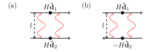
Figure 1: Schematic illustration of two interacting point electric dipoles (dots) with magnitude $H$ and orientation vectors ${\bf d}_{1}$ and ${\bf d}_{2}$, separated by a distance $l$. In (a) we show the symmetric and in (b) the antisymmetric excitation.

The decay rate of an electric dipole,

$$\Gamma^{(1)}=\Gamma_{\text{O}}+\Gamma_{\text{E1}}\,\text{,}$$ (103)

depends on the rate of dipole radiation and nonradiative losses that we set to $\Gamma_{\text{E1}}=0.83\Gamma^{(1)}$ and $\Gamma_{\text{O}}=0.17\Gamma^{(1)}$.

When the driving field is tuned to the resonance frequency of the point electric dipoles, $\Omega_{0}=\omega_{0}$, the coupling matrix in the equation of motion [Eq. (52), with $\Gamma_{\text{M1}}\equiv\Gamma_{\text{E2}}\equiv 0$], of a pair of electric dipoles is,

$$\mathcal{C}=\begin{bmatrix}-\dfrac{\Gamma^{(1)}}{2}&i\dfrac{3}{4}\Gamma_{\text{E1}}G_{\text{E1}}({\bf r}_{12})\\ i\dfrac{3}{4}\Gamma_{\text{E1}}G_{\text{E1}}(-{\bf r}_{12})&-\dfrac{\Gamma^{(1)}}{2}\end{bmatrix}\,\text{,}$$ (104)

where $\Gamma^{(1)}=\Gamma_{\text{O}}+\Gamma_{\text{E1}}$ [see Eq. (103)], ${\bf r}_{12}={\bf r}_{2}-{\bf r}_{1}$, and $G_{\text{E1}}({\bf r}_{12})=G_{\text{E1}}(-{\bf r}_{12})$, which from Eq. (5)

$$G_{\text{E1}}({\bf r}_{12})=\frac{i}{3}\left[2h_{0}^{(1)}(kl)-h_{2}^{(1)}(kl)\right]\,\text{.}$$ (105)

Equation (104) has two eigenmodes of current oscillation: a symmetric mode (denoted by a subscript ‘s’), where both dipoles current oscillations are in phase, i.e., ${\bf\hat{d}}_{1}={\bf\hat{d}}_{2}$, see Fig. 1(a); and an antisymmetric mode (denoted by a subscript ‘a’), where the current oscillations of the dipoles are out of phase, i.e., ${\bf\hat{d}}_{1}=-{\bf\hat{d}}_{2}$, see Fig. 1(b). The eigenvectors (${\bf v}_{n}^{(1)}$) and corresponding eigenvalues ($\xi_{n}^{(1)}$) of the the two modes of current oscillation are

$${\bf v}_{\text{s}}^{(1)}=\frac{1}{\sqrt{2}}\begin{bmatrix}1\\ 1\end{bmatrix}\quad\text{and}\quad{\bf v}_{\text{a}}^{(1)}=\frac{1}{\sqrt{2}}\begin{bmatrix}1\\ -1\end{bmatrix}\,\text{,}$$ (106)

and eigenvalues

$$\xi_{\text{a,s}}^{(1)}=-\frac{\Gamma^{(1)}}{2}\pm i\frac{3}{4}\Gamma_{\text{E1}}G_{\text{E1}}({\bf r}_{12})\,\text{,}$$ (107)

respectively. The eigenvalues determine the mode resonance frequency shifts $\delta\omega_{\text{a,s}}^{(1)}=-(\Omega_{\text{a,s}}^{(1)}-\Omega_{0})=\text{Im}(\xi_{\text{a,s}}^{(1)})$, and mode decay rates $\gamma_{\text{a,s}}^{(1)}=2\text{Re}(\xi_{\text{a,s}}^{(1)})$, see Eq. (29). We will later use the symmetric and antisymmetric mode decay rates $\gamma_{\text{s}}^{(1)}$ and $\gamma_{\text{a}}^{(1)}$, and the corresponding line shifts $\delta\omega_{\text{s}}^{(1)}$ and $\delta\omega_{\text{a}}^{(1)}$, as estimates for the total decay rates and resonance frequencies of a single point emitter possessing either electric dipole or both magnetic dipole and electric quadrupole moments.

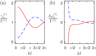
Figure 2: The radiative resonance (a) linewidths and (b) line shifts for the collective antisymmetric (blue dashed line) and symmetric (red solid line) eigenmodes, as a function of the separation $l$, for two parallel point electric dipoles. The radiative losses of each dipole are $\Gamma_{\text{E1}}=0.83\Gamma^{(1)}$, the ohmic losses are $\Gamma_{\text{O}}=0.17\Gamma^{(1)}$.

In Fig. 2 we show the radiative resonance linewidths and line shifts for the collective antisymmetric and symmetric eigenmodes. As the separation because small $l\rightarrow 0$, the linewidth of the antisymmetric mode approaches the ohmic loss rate ($\gamma_{\text{a}}^{(1)}\rightarrow\Gamma_{\text{O}}$) and is subradiant, the symmetric mode linewidth approaches $\gamma_{\text{s}}^{(1)}\rightarrow 1.8\Gamma^{(1)}$ and is superradiant. At approximately $kl\approx\pi$ (where $k=2\pi/\lambda_{0}$), the symmetric and antisymmetric modes become subradiant and superradiant, respectively. The line shifts of two modes are symmetric about $\Omega_{0}$. At $kl\approx\pi/4$, the line shifts diverge with $\delta\omega_{\text{s}}^{(1)}$ red shifted, and $\delta\omega_{\text{a}}^{(1)}$ blue shifted, from $\Omega_{0}$.

V.2 Effective point emitter for a pair of out-of-phase electric dipoles

Two closely-spaced parallel electric dipoles have eigenmodes that represent in-phase and out-of-phase excitations Eq. (106). The in-phase oscillations of a pair of dipoles can be approximated by a single electric dipole point emitter. For the antisymmetric, out-of-phase oscillations the total electric dipole is weak, but the pair exhibits nonvanishing electric quadrupole and magnetic dipole moments (see Fig. 3). We therefore approximate a pair of closely-spaced, parallel out-of-phase point electric dipoles by a single point emitter, possessing a magnetic dipole and electric quadrupole moment, located between the two electric dipoles.

We write the decay rate of a point emitter corresponding to the pair of out-of-phase electric dipoles as

$$\gamma_{\text{a}}^{(1)}=\Gamma_{\text{O}}+\Gamma_{\text{M1}}+\Gamma_{\text{E2}}\,\text{,}$$ (108)

where the antisymmetric collective mode linewidth $\gamma_{\text{a}}^{(1)}$ of two parallel electric dipoles can be calculated and is shown in Fig. 2. Using this formula, we may then derive analytical expressions for $\Gamma_{\text{M1}}$ and $\Gamma_{\text{E2}}$.

Figure 3: Schematic illustration of the effective magnetic dipole moment [pointing into the page] and electric quadrupole moment, both located at the center of the cross, formed by two parallel antisymmetrically excited point electric dipoles (dots), with magnitude $H$ and orientation vectors $\pm{\bf\hat{d}}$, separated by a distance $l$.

Also shown in Fig. 2, is the antisymmetric collective mode line shift $\delta\omega_{\text{a}}^{(1)}$. The resonance frequency of the magnetic dipole and electric quadrupole resonator $\Omega_{\text{a}}^{(1)}$, is related to the line shift of the antisymmetric mode of two parallel electric dipoles by

$$\Omega_{\text{a}}^{(1)}=(\Omega_{0}-\delta\omega_{\text{a}}^{(1)})\,\text{.}$$ (109)

V.2.1 Magnetic dipole moment of two parallel electric dipoles

In Sec. III and Ref. 6, the magnetic dipole moment arose solely due to the magnetization ${\bf M}_{j}({\bf r},t)$. We assume the resonator $j$ comprises two electric dipoles located at ${\bf r}_{\pm,j}=[x_{j},y_{j}\pm l_{j}/2,z_{j}]$, where $l_{j}\ll\lambda_{0}$, with linear charge and current oscillations along their axes. An effective magnetization ${\bf M}_{\text{P},j}({\bf r},t)$ is present due to the polarization of the two parallel electric dipoles, where

$${\bf M}_{\text{P},j}({\bf r},t)=I_{j}(t){\bf\bar{w}}_{j}({\bf r})\,\text{,}$$ (110)

where ${\bf\bar{w}}_{j}({\bf r})$ is the effective current profile function. The scattered EM fields due to the effective magnetic source located at ${\bf r}^{\prime}$, follow from the EM fields, Eqs. (3) and (4), with the effective magnetization Eq. (110).

In the point magnetic dipole approximation, the spatial profile function ${\bf\bar{w}}_{j}({\bf r})$ of the effective magnetization is approximated as a delta function at the origin

$${\bf\bar{w}}_{j}({\bf r}) =\frac{1}{2}\int\text{d}^{3}r\,({\bf r}-{\bf r}_{j})\times\big{[}{\bf p}_{+,j}({\bf r})+{\bf p}_{-,j}({\bf r})\big{]}$$

$$\simeq A_{\text{M},j}{\bf\hat{m}}_{j}\delta({\bf r}-{\bf r}_{j})\,\text{.}$$ (111)

The effective area $A_{\text{M},j}$, of the point magnetic dipole [see Fig. 3] may be approximated by evaluating Eq. (111) with ${\bf p}_{\pm,j}({\bf r})=\pm H{\bf\hat{d}}\delta({\bf r}-{\bf r}_{\pm,j})$. We find the point magnetic dipole moment, of the $j$th pair of antisymmetrically excited point electric dipoles, has an effective area

$$A_{\text{M},j}=\frac{l_{j}H_{j}}{2}\,\text{.}$$ (112)

The magnetic dipole decay rate is dependent upon the magnitude of the electric dipoles $H_{j}$ which comprise the pair, and their separation $l_{j}$, i.e., their effective cross sectional area.

If the two electric point dipoles are not extremely close to each other, the resonance frequency of the antisymmetric mode is close to that of the single isolated electric dipole. We use the same resonance frequency (Eq. (9)) in both Eqs. (32) and (33), together with the effective area of the magnetic dipole Eq. (112), to find the ratio of the two emission rates is approximately given by

$$\Gamma_{\text{M1}}=\frac{\pi^{2}l_{j}^{2}}{\lambda^{2}}\Gamma_{\text{E1}}\,\text{.}$$ (113)

V.2.2 Electric quadrupole moment of two parallel electric dipoles

The effective area of the point electric quadrupole is obtained from a pair of out-of-phase point electric dipoles. We compare Eq. (65) (using the charge density of the electric dipoles, i.e., $\rho_{j}({\bf r},t)=-Q\nabla\cdotp{\bf p}^{\text{d}}_{j}({\bf r})$) with Eq. (72) to obtain the effective area

$$A_{\alpha\beta,j}=-\sum_{\pm}\int\text{d}^{3}r^{\prime}\,r_{\alpha}r_{\beta}\frac{\partial}{\partial r_{\gamma}}p_{\gamma}^{\text{d},\pm}({\bf r}^{\prime})\,\text{,}$$ (114)

where ${\bf r}^{\prime}={\bf r}-{\bf r}_{j}$ and the summation is over each of the $\pm$ orientated electric dipoles. Integrating Eq. (114) by parts results in Kronecker $\delta$ functions, see e.g., Eq. (73), and we find

$$A_{\alpha\beta,j}=\sum_{\pm}\int\text{d}^{3}r^{\prime}\,\Big{[}r^{\prime}_{\beta}p^{\text{d},\pm}_{\alpha,j}({\bf r^{\prime}})+r^{\prime}_{\alpha}p^{\text{d},\pm}_{\beta,j}({\bf r^{\prime}})\Big{]}\,\text{.}$$ (115)

For an electric dipole pair separated by $l$ along the $y$ axis (Fig. 3), the dipoles are perpendicular to ${\bf\hat{y}}$, i.e., ${\bf\hat{d}}_{j}^{\pm}=\pm{\bf\hat{y}}_{\perp}$. By symmetry, all elements of the tensor $A_{\alpha\beta,j}$ are zero, with the exception of $A_{y\hat{d},j}=A_{\hat{d}y,j}$. For example, let the electric dipoles be aligned along the $x$ axis. Then, two antisymmetrically excited point electric dipoles located at ${\bf r}_{\pm,j}=[x_{j},y_{j}\pm l_{j}/2,z_{j}]$, have mode functions ${\bf p}^{\text{d},\pm}_{j}({\bf r})=\pm H_{j}{\bf\hat{x}}\delta({\bf r}-{\bf r}_{\pm,j})$. The nonzero components of Eq. (115) are

$$A_{yx,j}=A_{xy,j}=\int\text{d}^{3}r^{\prime}\,\Big{[}r^{\prime}_{y}p_{x,j}^{\text{d},+}({\bf r}^{\prime})-r^{\prime}_{y}p_{x,j}^{\text{d},-}({\bf r}^{\prime})\Big{]}\,\text{.}$$ (116)

The integral in Eq. (116) is carried out over the $\delta$ function, and summing over the indices $\alpha,\beta$ in Eq. (78) provides the effective area of our point electric quadrupole

$$A_{\text{E},j}=\sqrt{2}l_{j}H_{j}\,\text{.}$$ (117)

The electric quadrupole radiative emission rate also depends on the amplitudes of the point electric dipoles and their separation. If the electric dipoles are symmetrically excited, then one may readily verify the point electric quadrupole moment vanishes.

In the examples in this section, the radiative emission rates of the magnetic dipole and the electric quadrupole both depend the effective area of a pair of parallel electric dipoles. We assume that resonance frequencies of the magnetic dipole and electric quadrupole moments of the $j$th source are $\omega_{j}$, [Eq. (9)]. The relative decay rate of the magnetic dipole and electric quadrupole, Eq. (80), depends on the effective areas, $A_{\text{M},j}$ and $A_{\text{E},j}$, Eqs. (112) and (117), respectively. We find the relative radiation rates for our example are

$$\Gamma_{\text{E2}}=\frac{12}{5}\Gamma_{\text{M1}}\,\text{.}$$ (118)

The radiative emission rate of an isolated point electric quadrupole may be related to the point electric dipole through Eq. (113).

V.3 Two interacting pairs of point electric dipoles

In this section, we illustrate and test the effective point emitter model for the system of two pairs of parallel electric point dipoles by describing each pair by an effective scatterer possessing an electric dipole or a magnetic dipole and electric quadrupole moments. We consider two geometries: two horizontal parallel pairs [Fig. 4(a)] and two perpendicular parallel pairs [Fig. 9(a)].

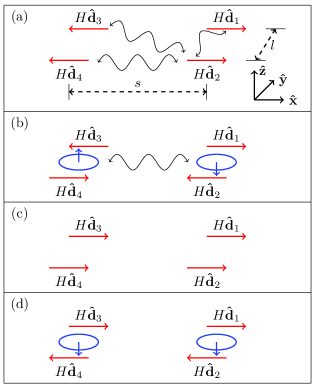
Figure 4: Schematic illustration of the eigenmodes of two horizontal pairs of parallel electric dipoles. The loops illustrate induced effective magnetic dipoles of each pair. The separation between the pairs is denoted by $s$ and the separation between the dipoles within each pair by $l$. We show the modes: (a) E1a; (b) M1E2a; (c) E1s; and (d) M1E2s.

From the coupling matrix Eq. (104) we obtain four collective eigenmodes of current oscillation. We classify the modes as (see Figs. 4 and 9): antisymmetric electric dipoles (E1a); antisymmetric magnetic dipole–electric quadrupoles (M1E2a); symmetric electric dipoles (E1s); and symmetric magnetic dipole–electric quadrupoles (M1E2s). In the E1a and E1s modes each parallel pair of resonators forms an effective electric dipole. However, in the E1a mode the current oscillations in the different parallel pairs are out of phase, and in the E1s mode they are in phase. In the M1E2a and M1E2s modes, the pairs form effective magnetic dipoles.

In the remainder of this section we will directly compare the E1a, E1s modes of the four point electric dipoles (denoted by a superscript (1)) to an corresponding modes of an effective electric dipole model (denoted by a superscript (2s)). We also compare the M1E2a and M1E2s modes of the four point electric dipoles (also denoted by a superscript (1)) to an effective magnetic dipole-electric quadrupole model (denoted by a superscript (2a)).

V.3.1 Description of electric dipoles by two multipole point emitters

In general, the $j$th pair of parallel electric dipoles are located at ${\bf r}_{\pm,j}=[x_{j},y_{j}\pm l/2,z_{j}]$. When the separation $l$, between parallel electric dipoles is small, the $j$th pair may be approximated by a single resonator located at ${\bf r}_{j}=[x_{j},y_{j},z_{j}]$.

When each parallel pair of electric dipoles are symmetrically excited [see, e.g., Fig. 4(a,c)], each pair may be approximated by a single point electric dipole, located at the center of the pair. We introduced the interactions between two point electric dipoles in Sec. V.1. We may use similar analysis to model the symmetric (E1s and E1a) collective modes of two interacting pairs of electric dipoles. The coupling matrix in this case is given by Eq. (104); with $\Gamma^{(1)}\rightarrow\gamma_{\text{s}}^{(1)}$ and the driving field is tuned to the resonance frequency of the symmetrically excited pair of point electric dipoles, i.e, $\Omega_{0}=\Omega_{\text{s}}^{(1)}$. The eigenvectors of the effective electric dipole interaction matrix are

$${\bf v}^{\text{(2s)}}_{\text{E1s}}=\frac{1}{\sqrt{2}}\begin{bmatrix}1\\ 1\end{bmatrix}\quad\text{and}\quad{\bf v}^{\text{(2s)}}_{\text{E1a}}=\frac{1}{\sqrt{2}}\begin{bmatrix}1\\ -1\end{bmatrix}\,\text{.}$$ (119)

with corresponding eigenvalues $\xi^{\text{(2s)}}_{\text{E1s}}$ and $\xi^{\text{(2s)}}_{\text{E1a}}$, where

$$\xi_{\text{E1a,E1s}}^{\text{(2s)}}=-\frac{\gamma_{\text{s}}^{(1)}}{2}\pm\frac{3}{4}\Gamma_{\text{E1}}\mathcal{G}_{\text{E1}}({\bf r}_{12})\,\text{.}$$ (120)

Here, $\mathcal{G}_{\text{E1}}({\bf r}_{12})$ is defined in Eq. (105) and the argument ${\bf r}_{12}$ depends on the locations of the effective electric dipoles.

On the other hand, we argued in Sec. V.2 how a pair of antisymmetrically excited point electric dipoles can be approximated by a single point emitter possessing both magnetic dipole and electric quadrupole moments [see, e.g., Fig. 4(b,d)]. For two point emitters located at ${\bf r}_{1}$ and ${\bf r}_{2}$, with both magnetic dipole and electric quadrupole moments, the interaction matrix, $\mathcal{C}$, is

$$\mathcal{C}=\Delta^{\prime}-\frac{1}{2}\Upsilon+\frac{1}{2}\Big{[}i\mathcal{C}_{\text{M1}}+i\mathcal{C}_{\text{E2}}+\mathcal{C}_{\text{X2}}+\mathcal{C}_{\text{X2}}^{T}\Big{]}\,\text{.}$$ (121)

Similar to our example of two electric dipoles, the contributing matrices in Eq. (121) are also $2\times 2$. However, the off-diagonal elements of $\mathcal{C}$ are more complicated. In the diagonal elements, the total decay rate of each emitter is $\gamma^{(1)}_{\text{a}}$, given in Eq. (108). In general, the resonance frequency $\Omega^{(1)}_{\text{a}}\neq\omega_{0}$ [see Eq. (109)], thus $\Delta^{\prime}$ is not trivial and contains a frequency shift. The matrix contributions to $\mathcal{C}$ are then

$$\Delta^{\prime}= \begin{bmatrix}i\delta\omega_{\text{a}}^{(1)}&0\\ 0&i\delta\omega_{\text{a}}^{(1)}\end{bmatrix}\,\text{,}$$ (122)

$$\Upsilon= \begin{bmatrix}\gamma^{(1)}_{\text{a}}&0\\ 0&\gamma^{(1)}_{\text{a}}\end{bmatrix}\,\text{,}$$ (123)

$$\mathcal{C}_{\text{M1}}= \Gamma_{\text{M1}}\begin{bmatrix}0&G_{\text{M1}}({\bf r}_{12})\\ G_{\text{M1}}({\bf r}_{12})&0\end{bmatrix}\,\text{,}$$ (124)

$$\mathcal{C}_{\text{E2}}= \Gamma_{\text{E2}}\begin{bmatrix}0&G_{\text{E2}}({\bf r}_{12})\\ G_{\text{E2}}({\bf r}_{12})&0\end{bmatrix}\,\text{,}$$ (125)

$$\mathcal{C}_{\text{X2}}= \sqrt{\Gamma_{\text{M1}}\Gamma_{\text{E2}}}\begin{bmatrix}0&G_{\text{X2}}({\bf r}_{12})\\ G_{\text{X2}}({\bf r}_{12})&0\end{bmatrix}\,\text{,}$$ (126)

where ${G}_{\text{M1}}({\bf r}_{12})$, ${G}_{\text{E2}}({\bf r}_{12})$ and ${G}_{\text{X2}}({\bf r}_{12})$ depend exclusively on the orientations and locations of the magnetic dipoles and electric quadrupoles and we have utilized the symmetry property of the matrices, e.g., $[\mathcal{C}_{\text{M1}}]_{i,j}=[\mathcal{C}_{\text{M1}}]_{j,i}$, etc. The eigenvectors ${\bf v}_{n}^{(\text{2a})}$ of Eq. (121) are independent of the resonator locations, and correspond to symmetric and antisymmetric oscillations,

$${\bf v}_{\text{M1E2s}}^{(\text{2a})}=\frac{1}{\sqrt{2}}\begin{bmatrix}1\\ 1\end{bmatrix}\quad\text{and}\quad{\bf v}_{\text{M1E2a}}^{(\text{2a})}=\frac{1}{\sqrt{2}}\begin{bmatrix}1\\ -1\end{bmatrix}\,\text{.}$$ (127)

However, the eigenvalues $\xi_{n}^{(\text{2a})}$ of Eq. (121) depend on both the orientations and locations of the resonators. In the following section, we analyze in detail the point magnetic dipole and electric quadrupole interacting systems, utilizing the geometries introduced in Figs. 4 and 9.

V.3.2 Two horizontal pairs of point electric dipoles

When the point electric dipoles are arranged in horizontal pairs, the Cartesian coordinates of the electric dipoles are

$${\bf r}_{1,2}=\frac{1}{2}\begin{bmatrix}s\\ \pm l\\ 0\end{bmatrix}\,\text{,}\quad{\bf r}_{3,4}=\frac{1}{2}\begin{bmatrix}-s\\ \pm l\\ 0\end{bmatrix}\,\text{,}$$ (128)

The effective point emitters of these are then located at the center of each pair ${\bf r}_{1}=-{\bf r}_{2}=[s/2,0,0]$.

The interaction terms: ${G}_{\text{M1}}({\bf r}_{12})$; ${G}_{\text{E2}}({\bf r}_{12})$; and ${G}_{\text{X2}}({\bf r}_{12})$, in Eqs. (124)–(126), are given by

$$G_{\text{M1}}({\bf r}_{12}) =\frac{i}{2}\left[2h_{0}^{(1)}(ks)-h_{2}^{(1)}(ks)\right]\,\text{,}$$ (129)

$$G_{\text{E2}}({\bf r}_{12}) =-i\frac{5}{2}\Bigg{[}\frac{16}{35}h_{4}^{(1)}(ks)-\frac{3}{7}h_{2}^{(1)}(ks)+\frac{2}{5}h_{0}^{(1)}(ks)\Bigg{]}\,\text{,}$$ (130)

$$G_{\text{X2}}({\bf r}_{12}) =-\sqrt{\frac{15}{2}}h_{2}^{(1)}(ks)\,\text{,}$$ (131)

respectively. In this example, the eigenmodes correspond antisymmetric excitations (${\bf\hat{m}}_{1}=-{\bf\hat{m}}_{2}$, and $\hat{A}_{\alpha\beta,1}=-\hat{A}_{\alpha\beta,2}$), see Fig. 4(b), and to symmetric excitations of the resonators (${\bf\hat{m}}_{1}={\bf\hat{m}}_{2}$, and $\hat{A}_{\alpha\beta,1}=\hat{A}_{\alpha\beta,2}$), see Fig. 4(d). These eigenmodes are represented by the eigenvectors ${\bf v}_{\text{M1E2a}}^{(\text{2a})}$ and ${\bf v}_{\text{M1E2s}}^{(\text{2a})}$, respectively, given in Eq. (127). The eigenvalues $\xi_{\text{M1E2a}}^{(\text{2a})}$ and $\xi_{\text{M1E2s}}^{(\text{2a})}$, of Eq. (121) with Eqs. (129)–(131), are complicated and include contributions from $h_{4}^{(1)}(ks)$, $h_{2}^{(1)}(ks)$, and $h_{0}^{(1)}(ks)$. In the leading order expansion of the spherical Hankel functions, the real and imaginary parts of $\xi_{\text{M1E2a}}^{(\text{2a})}$ and $\xi_{\text{M1E2s}}^{(\text{2a})}$ are dominated by $h_{0}^{(1)}(ks)$ and $h_{4}^{(1)}(ks)$, respectively. Specifically, we find

$$\gamma_{\text{M1E2a}}^{(\text{2a})}= \text{Re}\big{(}\xi_{\text{M1E2a}}^{\text{(2a)}}\big{)}\approx-\frac{\gamma_{\text{a}}^{\text{(1)}}}{2}+\frac{1}{2}\Big{[}\Gamma_{\text{M1}}+\Gamma_{\text{E2}}\Big{]}\,\text{,}$$ (132a)

$$\gamma_{\text{M1E2s}}^{(\text{2a})}= \text{Re}\big{(}\xi_{\text{M1E2s}}^{\text{(2a)}}\big{)}\approx-\frac{\gamma_{\text{a}}^{\text{(1)}}}{2}-\frac{1}{2}\Big{[}\Gamma_{\text{M1}}+\Gamma_{\text{E2}}\Big{]}\,\text{,}$$ (132b)

$$\delta\omega^{\text{(2a)}}_{\text{M1E2a}} =\text{Im}\big{(}\xi_{\text{M1E2a}}^{\text{(2a)}}\big{)}\approx\delta\omega_{\text{a}}^{(1)}-\frac{240}{(ks)^{5}}\Gamma_{\text{E2}}\,\text{,}$$ (132c)

$$\delta\omega^{\text{(2a)}}_{\text{M1E2s}} =\text{Im}\big{(}\xi_{\text{M1E2s}}^{\text{(2a)}}\big{)}\approx\delta\omega_{\text{a}}^{(1)}+\frac{240}{(ks)^{5}}\Gamma_{\text{E2}}\,\text{.}$$ (132d)

Here, we have the antisymmetric collective mode decay rate $\gamma_{\text{M1E2a}}^{(\text{2a})}$ is subradiant approaching $\Gamma_{\text{O}}$, while the symmetric excitation is superradiant with $\gamma_{\text{M1E2s}}^{(\text{2a})}$ approaching $2\gamma^{(1)}_{\text{a}}$. When the resonators are close together, the line shifts of the collective modes are dominated by $\Gamma_{\text{E2}}$ and quickly diverge, with $\delta\omega^{\text{(2a)}}_{\text{M1E2a}}$ red shifted, and $\delta\omega^{\text{(2a)}}_{\text{M1E2s}}$ blue shifted, from $\delta\omega_{\text{a}}^{(1)}$.

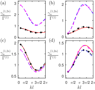
Figure 5: The radiative resonance linewidth $\gamma_{n}^{(\text{1,2s,2a})}$ for the collective eigenmodes as a function of the separation of dipoles within each pair $l$, for two horizontal pairs of point electric dipoles, with: (a) and (b) $ks=2\pi/3$; and (c) and (d) $ks=2\pi$. We show the linewidth $\gamma_{n}^{(1)}$ in the $N=4$ point electric dipole model, with the different modes shown as: E1a–red solid line (a) and (c); E1s–blue dashed line (a) and (c); M1E2a–red solid line (b) and (d); and M1E2s–blue dashed line (b) and (d). We show the linewidth $\gamma_{n}^{(\text{2s})}$ in the $N=2$ effective electric dipole resonator model: antisymmetric excitations–magenta dash circles (a) and (c); and symmetric excitations–black dash squares (a) and (c). The linewidth $\gamma_{n}^{(\text{2a})}$ in the $N=2$ effective magnetic dipole–electric quadrupole resonator model: antisymmetric excitations–magenta dash circles (b) and (d); and symmetric excitations–black dash squares (b) and (d). The radiative losses of each electric dipole are $\Gamma_{\text{E1}}=0.83\Gamma^{\text{(1)}}$, the ohmic losses are $\Gamma_{\text{O}}=0.17\Gamma^{\text{(1)}}$.

In Figs. 5 and 6, we show how the collective mode linewidths and line shifts, respectively, for the $N=4$ interacting point electric dipoles, vary with the separation of dipoles within each pair $l$, when $ks=2\pi/3$ and $ks=2\pi$. Also, in Figs. 5 and 6, we show the collective mode linewidths and line shifts for the effective $N=2$ multipole point emitters.

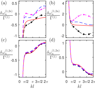
Figure 6: The radiative resonance line shift $\delta\omega_{n}^{(\text{1,2s,2a})}$ for the collective eigenmodes as a function of the separation parameter $l$, for two horizontal pairs of point electric dipoles, with: (a) and (b) $ks=2\pi/3$; and (c) and (d) $ks=2\pi$. For plot descriptions, see Fig. 5 caption.

When $l$ is varied, the linewidths $\gamma_{n}^{(\text{2s,2a})}$ of the $N=2$ effective multipole point emitters closely approximate the corresponding linewidths $\gamma_{n}^{(1)}$ of the $N=4$ point electric dipoles; both when $ks=2\pi/3$ and $ks=2\pi$. When $s$ is small [$ks=2\pi/3$, see Fig. 5(a) and 5(b)], the E1s mode is always superradiant, while both the E1a and M1E2a modes are always subradiant. When $s$ is small, the M1E2s mode exhibits both superradiant and subradiant behavior. For large $kl\gtrsim\pi/2$, we have superradiant behavior $\gamma_{\text{M1E2s}}^{(1)}>\Gamma^{(1)}$ and $kl\lesssim\pi/2$, subradiant behavior; $\gamma_{\text{M1E2s}}^{(1)}<\Gamma^{(1)}$. At the minimum value $\gamma_{\text{E1s}}^{(1)}\simeq 1.1\Gamma^{(1)}$. For large $s$ [see Fig. 5(c) and 5(d)], all the linewidths exhibit both superradiant and subradiant behavior.

While the collective mode linewidths resulting from the effective point emitter approximation qualitatively match those of the electric dipoles as $l$ varies at both large and small $s$, the corresponding line shifts show greater variations. In particular, when $ks=2\pi/3$, see Fig. 6(a) and 6(b), the collective line shifts $\delta\omega^{\text{(2a)}}_{\text{M1E2a}}$ and $\delta\omega^{(\text{2a})}_{\text{M1E2s}}$ begin to deviate from the corresponding line shifts $\delta\omega^{(1)}_{\text{M1E2a}}$ and $\delta\omega^{(1)}_{\text{M1E2s}}$, when $kl\simeq\pi/4$. When $kl\simeq\pi/4$, all the collective mode line shifts begin to significantly diverge as $l$ reduces further. In contrast, the E1a and E1s line shifts of the point electric dipole model qualitatively agree with the corresponding shifts of the effective multipole resonator model. When $s$ is large and $l$ is varied, there is no significant difference in the line shifts, even when $l$ is large. As we reduce the separation $l$, the line shifts $\delta\omega_{\text{E1a}}^{(1)}$ and $\delta\omega_{\text{E1s}}^{(1)}$ are red shifted from $\Omega_{0}$, see Fig. 6(a) and 6(c). In contrast, $\delta\omega_{\text{M1E2a}}^{(1)}$ and $\delta\omega_{\text{M1E2s}}^{(1)}$ are blue shifted, see Fig. 6(b) and 6(d).

In Fig. 7 we show analogous linewidths when the separation $s$ between the pairs is varied. The linewidths of the effective model again agree well with the full point dipole results. The antisymmetric mode linewidth approaches the nonradiative loss rate when both $l$ and $s$ are small $\gamma_{\text{M1E2s}}^{(1)}=\gamma_{\text{M1E2s}}^{(\text{2a})}\simeq\Gamma_{\text{O}}$, see Fig. 7(b).

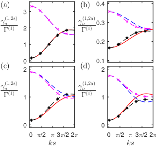
Figure 7: The resonance linewidth $\gamma_{n}^{(\text{1,2s,2a})}$ for the collective eigenmodes as a function of the separation parameter $s$, for two horizontal pairs of point electric dipoles, with: (a) and (b) $kl=\pi/4$; and (c) and (d) $kl=2\pi$. For plot descriptions, see Fig. 5 caption.

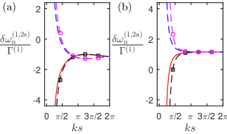
Figure 8: The resonance line shift $\delta\omega_{n}^{(\text{1,2s,2a})}$ for the collective eigenmodes as a function of the separation parameter $s$, for two horizontal pairs of point electric dipoles, with: (a) and (b) $kl=\pi/4$. For plot descriptions, see Fig. 6 caption.

In Fig. 8, we show the line shifts of the different collective modes as $s$ varies. The line shifts $\delta\omega_{\text{M1E2a}}^{(\text{2s})}$ and $\delta\omega_{\text{M1E2s}}^{\text{(2s)}}$, show no significant deviation from the E1a and E1s modes, even at small $s$ and $kl=\pi/4$. In contrast, the line shifts $\delta\omega_{\text{M1E2a}}^{\text{(2a)}}$ and $\delta\omega_{\text{M1E2s}}^{\text{(2a)}}$ begin to deviated from the M1E2a and M1E2s line shifts when $ks\simeq\pi/2$ (when $kl=\pi/4$).

V.3.3 Two perpendicular pairs of point electric dipoles

Our second example is two perpendicular pairs of point electric dipoles. The Cartesian coordinates of each electric dipole are

$${\bf r}_{1,2}=\begin{bmatrix}s\\ \pm\dfrac{l}{2}\\ 0\end{bmatrix}\,\text{,}\quad{\bf r}_{3,4}=\begin{bmatrix}0\\ \pm\dfrac{l}{2}\\ s\end{bmatrix}\,\text{.}$$ (133)

In Fig. 9(a) and 9(c), we show the E1a and E1s modes, respectively. In Fig. 9(b) and 9(d), we show the M1E2a and M1E2s modes, respectively. The locations vectors of the effective resonators with both point magnetic dipole and point electric quadrupole sources [and effective electric dipole sources] are ${\bf r}_{1}=[s,0,0]$ and ${\bf r}_{2}=[0,0,s]$.

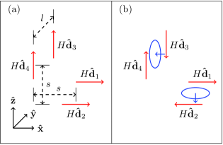
Figure 9: A schematic illustration of two perpendicular pairs of electric dipoles and the induced effective magnetic dipoles. The separation between dipoles within each pair is $l$ and the position of the pair on the $x,z$ axis is determined by $s$. We illustrate two of the four modes; see Fig. 4.

In this example, the magnetic dipole orientation vectors ${\bf\hat{m}}_{1,2}$ and the unit vector ${\bf\hat{k}}$ form an orthonormal set, i.e., ${\bf\hat{m}}_{1}=\pm{\bf\hat{k}}\times{\bf\hat{m}}_{2}$, corresponding to symmetric ($+$) and antisymmetric ($-$) oscillations, see Fig. 9(d), and 9(b), respectively. Similarly, the electric quadrupole unit tensors, for the symmetric ($+$) and antisymmetric ($-$) excitations are

$$\hat{A}_{1}=\begin{bmatrix}0&1&0\\ 1&0&0\\ 0&0&0\end{bmatrix}\quad\text{and}\quad\hat{A}_{2}=\pm\begin{bmatrix}0&0&0\\ 0&0&1\\ 0&1&0\end{bmatrix}\,\text{.}$$ (134)

These oscillations are represented through the eigenvectors ${\bf v}_{\text{M1E2s}}^{\text{(2a)}}$ and ${\bf v}_{\text{M1E2a}}^{\text{(2a)}}$, respectively, see Eq. (127). The interaction terms: ${G}_{\text{M1}}({\bf r}_{12})$; ${G}_{\text{E2}}({\bf r}_{12})$; and ${G}_{\text{X2}}({\bf r}_{12})$, in Eqs. (124)–(126), respectively, in this case are given by

$$G_{\text{M1}}({\bf r}_{12}) =i\frac{3}{4}h_{2}^{(1)}(\sqrt{2}ks)\,\text{,}$$ (135)

$$G_{\text{E2}}({\bf r}_{12}) =i\frac{20}{28}\Bigg{[}h_{4}^{(1)}(\sqrt{2}ks)-\frac{3}{4}h_{2}^{(1)}(\sqrt{2}ks)\Bigg{]}\,\text{,}$$ (136)

$$G_{\text{X2}}({\bf r}_{12}) =-\sqrt{\frac{15}{4}}h_{2}^{(1)}(\sqrt{2}ks)\,\text{.}$$ (137)

The eigenvalues $\xi_{\text{M1E2a}}^{\text{(2a)}}$ and $\xi_{\text{M1E2s}}^{\text{(2a)}}$ of Eq. (121), with Eqs. (135)–(137) are complex, involving contributions from $h_{4}^{(1)}(\sqrt{2}ks)$ and $h_{2}^{(1)}(\sqrt{2}ks)$. For analytical expressions of $\xi_{\text{M1E2a}}^{\text{(2a)}}$ and $\xi_{\text{M1E2s}}^{\text{(2a)}}$, we again consider the leading order expansions of the spherical Hankel functions. In this limit $\text{Im}(\xi_{n}^{\text{(2a)}})$ is dominated by $h_{4}^{(1)}(\sqrt{2}ks)$ and $\text{Re}(\xi_{n}^{\text{(2a)}})$ by $h_{2}^{(1)}(\sqrt{2}ks)$. Specifically, we find

$$\delta\omega^{\text{(2a)}}_{\text{M1E2a}}= \,\text{Im}\big{(}\xi_{\text{M1E2a}}^{\text{(2a)}}\big{)}\approx\delta\omega_{\text{a}}^{(1)}+\frac{1125}{(\sqrt{2}ks)^{5}}\Gamma_{\text{E2}}\,\text{,}$$ (138a)

$$\delta\omega^{\text{(2a)}}_{\text{M1E2s}}= \,\text{Im}\big{(}\xi_{\text{M1E2s}}^{\text{(2a)}}\big{)}\approx\delta\omega_{\text{a}}^{(1)}-\frac{1125}{(\sqrt{2}ks)^{5}}\Gamma_{\text{E2}}\,\text{,}$$ (138b)

$$\gamma^{\text{(2a)}}_{\text{M1E2a}}= \,\text{Re}\big{(}\xi_{\text{M1E2a}}^{\text{(2a)}}\big{)}\approx-\frac{\gamma^{(1)}_{\text{a}}}{2}+\bigg{[}\frac{\Gamma_{\text{M1}}}{10}+\frac{\Gamma_{\text{E2}}}{28}$$

$$\quad+\sqrt{\frac{15}{4}}\sqrt{\Gamma_{\text{M1}}\Gamma_{\text{E2}}}\bigg{]}(\sqrt{2}ks)^{2}\,\text{,}$$ (138c)

$$\gamma^{\text{(2a)}}_{\text{M1E2s}}= \,\text{Re}\big{(}\xi_{\text{M1E2s}}^{\text{(2a)}}\big{)}\approx-\frac{\gamma^{(1)}_{\text{a}}}{2}-\bigg{[}\frac{\Gamma_{\text{M1}}}{10}+\frac{\Gamma_{\text{E2}}}{28}$$

$$\quad+\sqrt{\frac{15}{4}}\sqrt{\Gamma_{\text{M1}}\Gamma_{\text{E2}}}\bigg{]}(\sqrt{2}ks)^{2}\,\text{.}$$ (138d)

When the dipoles are close and perpendicular, they interact only weakly, $\gamma_{\text{M1E2a}}^{\text{(2a)}}\approx\gamma_{\text{M1E2s}}^{\text{(2a)}}\approx\gamma^{(1)}_{\text{a}}$. The line shifts of the modes diverge as $ks\rightarrow 0$ and are dominated by $\Gamma_{\text{E2}}$, with $\delta\omega_{\text{M1E2a}}^{\text{(2a)}}$ blue shifted and $\delta\omega_{\text{M1E2s}}^{\text{(2a)}}$ red shifted from $\delta\omega_{\text{a}}^{(1)}$.

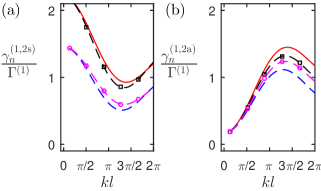
Figure 10: The radiative resonance linewidth $\gamma$ for the collective eigenmodes as a function of the separation parameter $l$, for two perpendicular pairs of point electric dipoles, with: (a) and (b) $ks=2\pi/5$. For plot descriptions, see Fig. 5 caption

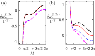
Figure 11: The radiative resonance line shift $\delta\omega$ for the collective eigenmodes as a function of the separation parameter $l$, for two perpendicular pairs of point electric dipoles, with: (a) and (b) $ks=2\pi/5$. For plot descriptions, see Fig. 6 caption

In Figs. 10 and 11, we show how the collective mode linewidths and line shifts, respectively, for situations similar to those of the parallel dipoles of Figs. 5 and 6, When $ks=2\pi/5$, and $l$ is varied, the linewidths of all the collective modes of perpendicular pairs closely resemble the linewidths of the corresponding horizontal pairs, see Figs. 10(a,b) and 5(c,d). There is no significant difference in the linewidths between the two different models, even when $s$ is small.

When we vary $s$ (Fig. 12), the perpendicular dipoles collective mode linewidths exhibit different behavior to those of horizontal dipoles, displaying characteristic oscillations as a function of the separation $s$. The effective multipole model provides a good approximation of the corresponding point electric dipole model linewidths. The line shifts of the perpendicular pairs have very similar characteristics to horizontal pairs, both when $s$ is large and when $s$ is small.

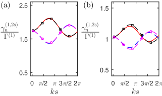
Figure 12: The resonance linewidth $\gamma$ for the collective eigenmodes as a function of the separation parameter $s$, for two perpendicular pairs of point electric dipoles with (a) $kl=\pi/4$ and (b) $kl=2\pi$. For plot descriptions, see Fig. 5 caption.

V.4 The response of an effective point emitter model to external fields

In this section, we compare the response of the four point electric dipole system with that of the effective two point emitter model under external driving, when we approximate the effective point emitter model with only one eigenmode. We consider the antisymmetric excitations, in which case the point emitter model exhibits the magnetic dipole and electric quadrupole moments. The driven dipoles radiate and induce excitations on the nearby dipoles, resulting in a strongly coupled system.

We solve the equation of motion Eq. (26) in a steady-state ($\dot{\bf b}=0$) for horizontal pairs of electric dipoles. We focus on the case when the external EM field drives one pair of dipoles only and propagates in the direction normal to the pair. For simplicity, we assume that the field perfectly couples to the antisymmetric excitation of the pair. In the point electric dipole system, we drive the pair 12, formed by the dipoles $n=1,2$. The driving by incident fields, ${\bf F}_{\text{in}}$ in Eq. (26), that takes the form

$${\bf F}_{\text{in}}=\frac{F_{0}}{\sqrt{2}}\begin{bmatrix}1\\ -1\\ 0\\ 0\end{bmatrix}\,\text{.}$$ (139)

We only take the antisymmetric mode for the $N=2$ effective point emitter system that exhibits magnetic dipole and electric quadrupole moments. The incident driving takes the form

$${\bf F}_{\text{in}}=F_{0}\begin{bmatrix}1\\ 0\end{bmatrix}\,\text{.}$$ (140)

The coupling matrix $\mathcal{C}$ in Eq. (26) is non-Hermitian, but we can define an occupation measure for a particular eigenmode ${\bf v}_{n}$ in an excitation ${\bf b}$ by

$${O}_{n}({\bf b})\equiv\left|{\bf v}_{n}^{T}{\bf b}\right|^{2}\,\text{.}$$ (141)

For the four electric dipoles, we project the excitation onto the basis

$${\bf v}_{12}^{(\pm)}=\frac{1}{\sqrt{2}}\begin{bmatrix}1\\ \pm 1\\ 0\\ 0\end{bmatrix}\,\text{,}\quad{\bf v}_{34}^{(\pm)}=\frac{1}{\sqrt{2}}\begin{bmatrix}0\\ 0\\ 1\\ \pm 1\end{bmatrix}\,\text{.}$$ (142)

Here, the superscript $(\pm)$ indicates symmetric/antisymmetric excitations of the dipole pair. In the effective two-emitter model we use the basis

$${\bf v}_{1}^{(-)}=\begin{bmatrix}1\\ 0\end{bmatrix}\,\text{,}\qquad{\bf v}_{2}^{(-)}=\begin{bmatrix}0\\ 1\end{bmatrix}\,\text{.}$$ (143)

In Fig. 13, we show the excitation spectra of the antisymmetric modes for the two models. For our choice of the driving in Eq. (139), the symmetric excitations of the electric dipoles are negligible. We find that, despite the inclusion of only one mode, the effective model agrees with the four-dipole case, provided that neither $s$ nor $l$ is too small. For small $s$ the geometry of the configuration starts becoming important, while for small $l$, the contribution of the symmetric excitations would need to be included. For $ks=4\pi/3$ and $kl=\pi/3$ (a,b), the effective model underestimates the excitation of the non-driven pair, while for $ks=8\pi/9$ and $kl=4\pi/9$ (c,d) the agreement is better.

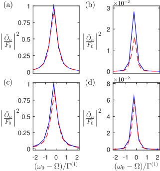
Figure 13: The excitation spectra of the antisymmetric modes of the electric dipole pairs (a,c) 1 and 2; (b,d) 3 and 4, as a function of the detuning of the incident frequency $\Omega$ from the resonance frequency $\omega_{0}$ of a single point electric dipole. The resonance is at $-(\omega_{0}-\Omega)\simeq 0.25\Gamma^{(1)}$. The full four point electric dipole model (blue solid line) and the corresponding effective two-point-emitter model, exhibiting magnetic dipole and electric quadrupole moments (red dashed line). In (a,b) $ks=4\pi/3$ and $kl=\pi/3$, (c,d) $ks=8\pi/11$ and $kl=8\pi/7$.

VI Conclusions

We have developed a formalism for effective point scatterer models that goes beyond the electric and magnetic dipole approximations, and also includes the more complicated electric quadrupole contributions to the interactions between the resonators. The resulting theory can then be expressed as a coupled set of dynamical equations for the resonators and EM fields. The interactions between the resonators result in collective eigenmodes with associative collective resonance frequency shifts and linewidths.

There is a clear motivation for introducing discrete models for the studies of EM field responses. For closely-spaced resonant emitters the EM-field-mediated interactions can be strong. The combination of recurrent scattering Wiersma et al. (1995); Ruostekoski and Javanainen (1997); Morice et al. (1995) – a process in which a wave is scattered more than once by the same emitter – and position-dependent radiative coupling between the emitters can lead to a correlated EM-field response. Even in a randomly distributed ensemble of emitters, such correlations have been shown to result in a qualitative failure of standard homogeneous-medium electrodynamics that, by construction, is a mean-field approximation Javanainen et al. (2014); Javanainen and Ruostekoski (2016). In large planar arrays of resonators, on the other hand, the collective effects can manifest themselves despite the presence of nonradiative losses, resulting, e.g., in a correlated excitation of a subradiant mode that can extend over the entire lattice, including over 1000 metamolecules Jenkins et al. (2016).

Here, we have tested and illustrated the effective theory using simple point scatterer models where we only include one mode of the corresponding two-point-dipole scatterer. The effective models could be extended to the studies of large arrays in which case they can provide considerable numerical simplifications, or also to the studies of more complex multipole resonatators Liu et al. (2009); Lovera et al. (2013); Fan et al. (2010); Hentschel et al. (2011); Frimmer et al. (2012); Dregely et al. (2011); Watson et al. (2016).

Appendix A Electric quadrupole radiation kernel

In Sec. IV, we calculated the EM fields scattered from a point electric quadrupole source, and the interaction between these scattered EM fields and other electric quadrupoles, electric dipoles and magnetic dipoles. The scattered EM fields and the resulting emf and flux terms contain derivatives of the radiation kernels Eqs. (5) and (6). In this Appendix, we give the corresponding derivatives of ${\bf G}({\bf r})$ and ${\bf G}_{\times}({\bf r})$.

The scattered electric ${\bf E}_{\text{E2},j}$ and magnetic ${\bf H}_{\text{E2},j}$ fields from the $j$th electric quadrupole are given in Eqs. (60) and (61). These equations contain rank three tensors which are the gradients of ${\bf G}({\bf r})$ and ${\bf G}_{\times}({\bf r})$, given by

$$\frac{\partial}{\partial kr_{\mu}}{\bf G}({\bf r}) =i\Bigg{[}\left[\frac{1}{5}\frac{r_{\mu}}{r}{\bf I}+\frac{1}{5}\frac{{\bf r}{\bf\hat{r}}_{\mu}+{\bf\hat{r}}_{\mu}{\bf r}}{r}-\frac{r_{\mu}}{r}\frac{{\bf r}{\bf r}}{r^{2}}\right]h_{3}^{(1)}(kr)-\left[\frac{12}{15}\frac{r_{\mu}}{r}{\bf I}-\frac{1}{5}\frac{{\bf r}{\bf\hat{r}}_{\mu}+{\bf\hat{r}}_{\mu}{\bf r}}{r}\right]h_{1}^{(1)}(kr)\Bigg{]}\,\text{,}$$ (144)

$$\frac{\partial}{\partial kr_{\mu}}{\bf G}_{\times}({\bf r}) =\frac{1}{r^{2}}\left[r_{\eta}{\bf\hat{r}}_{\nu}\left({\bf r}_{\mu}+{\bf r}_{\nu}+{\bf r}_{\eta}\right)-r_{\nu}({\bf\hat{r}}_{\eta}\left({\bf r}_{\mu}+{\bf r}_{\nu}+{\bf r}_{\eta}\right)\right]h_{2}^{(1)}(kr)-\frac{1}{r}\left[{\bf\hat{r}}_{\nu}{\bf\hat{r}}_{\eta}-{\bf\hat{r}}_{\eta}{\bf\hat{r}}_{\nu}\right]h_{1}^{(1)}(kr)\,\text{.}$$ (145)

Here: $r_{\mu}$ is Cartesian component $\mu=x,y,z$ of the vector ${\bf r}$; ${\bf r}{\bf r}$ is the outer product of ${\bf r}$ with itself; ${\bf I}$ is the identity matrix; and ${\bf\hat{r}}_{\mu}{\bf r}$ is the outer product of the unit vector ${\bf\hat{r}}_{\mu}$ in the Cartesian direction $\mu=x,y,z$ with the vector ${\bf r}$; and $h_{n}^{(1)}(kr)$ are the $n$th order spherical Hankel functions of the first kind, defined by

$$h_{1}^{(1)}(x) =-\left[1+\frac{i}{x}\right]\frac{e^{ix}}{x}\,\text{,}$$ (146)

$$h_{3}^{(1)}(x) =\left[1+\frac{6i}{x}-\frac{15}{x^{2}}-\frac{15i}{x^{3}}\right]\frac{e^{ix}}{x}\,\text{,}$$ (147)

$h_{2}^{(1)}(x)$ is defined in Eq. (8). In the cross kernel derivatives, Eq. (145), the component $\partial r_{\mu}G_{\times,\mu\nu}({\bf r})=0$ for $\nu=\mu,\nu,\eta$.

The interaction between two separate electric quadrupoles $i$ and $j$ results in an effective emf $\mathcal{E}_{i,j}^{\text{sc,E2}}$, see Eqs. (90)–(92). Equation (92) describes the interaction matrix $\mathcal{G}_{\text{E2}}$ whose off-diagonal elements represent the interactions between two electric quadrupoles, taking into account their relative locations and orientations only. $\mathcal{G}_{\text{E2}}$ is a contraction of the quadrupole moment tensors $\hat{A}_{\alpha\beta,m}$ and $\hat{A}_{\mu\nu,n}$ and a rank four tensor. The rank four tensor contains second order derivatives of ${\bf G}({\bf r})$,

$$\frac{\partial^{2}}{\partial kr_{\mu}\partial kr_{\mu}} \bigg{|}_{r_{\mu}=r_{\mu}}{\bf G}({\bf r})=i\Bigg{\{}\left[\frac{r_{\mu}^{2}}{r^{4}}{\bf r}{\bf r}-\frac{1}{7r^{2}}\left({\bf r}{\bf r}+r_{\mu}^{2}{\bf I}-4{\bf\hat{r}}_{\mu}{\bf\hat{r}}_{\mu}-2\left[{\bf r}_{\mu}{\bf r}_{\nu}+{\bf r}_{\nu}{\bf r}_{\mu}\right]\right)+\frac{1}{35}\left({\bf I}+2{\bf\hat{r}}_{\mu}{\bf\hat{r}}_{\mu}\right)\right]h_{4}^{(1)}(kr)$$

$$-\left[\frac{1}{7r^{2}}\left[{\bf r}{\bf r}+2\left({\bf r}_{\mu}{\bf r}_{\nu}+{\bf r}_{\nu}{\bf r}_{\mu}\right)+r_{\mu}^{2}{\bf I}+3{\bf r}_{\mu}{\bf r}_{\mu}\right]+\frac{5}{21}\left({\bf I}+4{\bf\hat{r}}_{\mu}{\bf\hat{r}}_{\mu}\right)\right]h_{2}^{(1)}(kr)-\frac{4}{15}\left[{\bf I}+2{\bf\hat{r}}_{\mu}{\bf\hat{r}}_{\mu}\right]h_{0}^{(1)}(kr)\Bigg{\}}\,\text{.}$$ (148)

$$\frac{\partial^{2}}{\partial kr_{\mu}\partial kr_{\nu}} \bigg{|}_{r_{\mu}\neq r_{\nu}}{\bf G}({\bf r})=i\Bigg{\{}\left[\frac{r_{\mu}r_{\nu}}{r^{4}}{\bf r}{\bf r}-\frac{1}{7r^{2}}\left[r_{\mu}\left({\bf r}{\bf\hat{r}}_{\nu}+{\bf\hat{r}}_{\nu}{\bf r}\right)+r_{\nu}\left({\bf r}{\bf\hat{r}}_{\mu}+{\bf\hat{r}}_{\mu}{\bf r}\right)+r_{\mu}r_{\nu}{\bf I}\right]+\frac{1}{35}\left({\bf\hat{r}}_{\mu}{\bf\hat{r}}_{\nu}+{\bf\hat{r}}_{\nu}{\bf\hat{r}}_{\mu}\right)\right]h_{4}^{(1)}(kr)$$

$$-\left[\frac{1}{7r^{2}}\left(r_{\mu}\left[{\bf r}{\bf\hat{r}}_{\nu}+{\bf\hat{r}}_{\nu}{\bf r}\right]+r_{\nu}\left[{\bf r}{\bf\hat{r}}_{\mu}+{\bf\hat{r}}_{\mu}{\bf r}-6r_{\mu}{\bf I}\right]\right)-\frac{2}{21}\left({\bf\hat{r}}_{\mu}{\bf\hat{r}}_{\nu}+{\bf\hat{r}}_{\nu}{\bf\hat{r}}_{\mu}\right)\right]h_{2}^{(1)}(kr)+\frac{1}{15}\left[{\bf\hat{r}}_{\mu}{\bf\hat{r}}_{\nu}+{\bf\hat{r}}_{\nu}{\bf\hat{r}}_{\mu}\right]h_{0}^{(1)}(kr)\Bigg{\}}\,\text{.}$$ (149)

The spherical Hankel functions $h_{0}^{(1)}(kr)$ and $h_{2}^{(1)}(kr)$ are defined in Eqs. (7) and (8), respectively, while

$$h_{4}^{(1)}(x)=-i\left[1+\frac{10i}{x}-\frac{45}{x^{2}}-\frac{105i}{x^{3}}+\frac{105}{x^{4}}\right]\frac{e^{ix}}{x}\,\text{.}$$ (150)

A.1 Electric quadrupole radiated power

In Sec. IV, we obtain an expression for the electric quadrupole radiative emission rate $\Gamma_{\text{E2},j}$, by calculating the radiated power $P_{\text{E2}}$, see Eqs. (68) and (69). To arrive at Eq. (69), we had to evaluate the integral of $|{\bf\hat{r}}\times{\bf q}_{j}({\bf\hat{r}})|^{2}$, over all angles. To do so, we note the Cartesian coordinate identity Zangwill (2013)

$$|{\bf\hat{r}}\times{\bf q}_{j}({\bf\hat{r}})|^{2} =\sum_{\alpha\beta\eta}q_{\alpha\beta,j}\hat{r}_{\beta}q_{\alpha\eta,n}^{\ast}\hat{r}_{\eta}$$

$$\quad\quad-\sum_{\alpha\beta\eta\nu}\hat{r}_{\alpha}q_{\alpha\beta,j}\hat{r}_{\beta}\hat{r}_{\eta}q_{\eta\nu,n}^{\ast}\hat{r}_{\nu}\,\text{.}$$ (151)

The different ${\hat{r}}_{\alpha}$’s are direction cosines which obey the identities Zangwill (2013)

$$\int\text{d}\Omega\,{\hat{r}}_{\beta}{\hat{r}}_{\eta} =\frac{4\pi}{3}\delta_{\beta\eta}\,\text{,}$$ (152)

$$\int\text{d}\Omega\,{\hat{r}}_{\alpha}{\hat{r}}_{\beta}{\hat{r}}_{\eta}{\hat{r}}_{\nu} =\frac{4\pi}{15}\Big{[}\delta_{\alpha\beta}\delta_{\eta\nu}+\delta_{\alpha\eta}\delta_{\beta\nu}+\delta_{\alpha\nu}\delta_{\beta\eta}\Big{]}\,\text{.}$$ (153)

Evaluating the integrals in Eqs. (152) and (153), and summing over the Cartesian indices $x$, $y$ and $z$, hence results in Eq. (69).

References

- Szabo et al. (2010) Z. Szabo, Gi-Ho Park, R. Hedge, and Er-Ping Li, “A unique extraction of metamaterial parameters based on kramers - kronig relationship,” IEEE Trans. Microwave Theory Tech. 58, 2646–2653 (2010).
- Koschny et al. (2004) T. Koschny, M. Kafesaki, E. N. Economou, and C. M. Soukoulis, “Effective medium theory of left-handed materials,” Phys. Rev. Lett. 93, 107402 (2004).
- Pendry et al. (1999) J. B. Pendry, A. J. Holden, D. J. Robbins, and W. J. Stewart, “Magnetism from conductors and enhanced nonlinear phenomena,” IEEE Transactions on Microwave Theory and Techniques 47, 2075 (1999).
- Belov and Simovski (2005) Pavel A. Belov and Constantin R. Simovski, “Homogenization of electromagnetic crystals formed by uniaxial resonant scatterers,” Phys. Rev. E 72, 026615 (2005).
- Liu et al. (2007) Ruopeng Liu, Tie Jun Cui, Da Huang, Bo Zhao, and David R. Smith, “Description and explanation of electromagnetic behaviors in artificial metamaterials based on effective medium theory,” Phys. Rev. E 76, 026606 (2007).
- Jenkins and Ruostekoski (2012a) S. D. Jenkins and J. Ruostekoski, “Theoretical formalism for collective electromagnetic response of discrete metamaterial systems,” Phys. Rev. B 86, 085116 (2012a).
- de Vries et al. (1998) Pedro de Vries, David V. van Coevorden, and Ad Lagendijk, “Point scatterers for classical waves,” Rev. Mod. Phys. 70, 447–466 (1998).
- Mühlschlegel et al. (2005) P. Mühlschlegel, H.-J. Eisler, O. J. F. Martin, B. Hecht, and D. W. Pohl, “Resonant optical antennas,” Science 308, 1607–1609 (2005), http://science.sciencemag.org/content/308/5728/1607.full.pdf .
- Fromm et al. (2004) David P. Fromm, Arvind Sundaramurthy, P. James Schuck, Gordon Kino, and W. E. Moerner, “Gap-dependent optical coupling of single €“bowtie”€ nanoantennas resonant in the visible,” Nano Letters 4, 957–961 (2004), http://dx.doi.org/10.1021/nl049951r .
- Evlyukhin et al. (2010) Andrey B. Evlyukhin, Carsten Reinhardt, Andreas Seidel, Boris S. Luk’yanchuk, and Boris N. Chichkov, “Optical response features of si-nanoparticle arrays,” Phys. Rev. B 82, 045404 (2010).
- Wang et al. (2011) Meng Wang, Min Cao, Xin Chen, and Ning Gu, “Subradiant plasmon modes in multilayer metal-€“dielectric nanoshells,” The Journal of Physical Chemistry C 115, 20920–20925 (2011), http://dx.doi.org/10.1021/jp205736d .
- Jenkins and Ruostekoski (2012b) S. D. Jenkins and J. Ruostekoski, “Cooperative resonance linewidth narrowing in a planar metamaterial,” New Journal of Physics 14, 103003 (2012b).
- Jenkins and Ruostekoski (2013) S. D. Jenkins and J. Ruostekoski, “Metamaterial transparency induced by cooperative electromagnetic interactions,” Phys. Rev. Lett. 111, 147401 (2013).
- Jenkins et al. (2016) S. D. Jenkins, J. Ruostekoski, N. Papasimakis, S. Savo, and N. I. Zheludev, “Many-body subradiant excitations in metamaterial arrays: Experiment and theory, eprint arxiv:1611.01509,” (2016).
- Smith et al. (2000) D. R. Smith, W. J. Padilla, D. C. Vier, S. C. Nemat-Nasser, and S. Schultz, “Composite medium with simultaneously negative permeability and permittivity,” Phys. Rev. Lett. 84, 4184 (2000).
- Fedotov et al. (2007) V. A. Fedotov, M. Rose, S. L. Prosvirnin, N. Papasimakis, and N. I. Zheludev, “Sharp trapped-mode resonances in planar metamaterials with a broken structural symmetry,” Phys. Rev. Lett. 99, 147401 (2007).
- Adamo et al. (2012) G. Adamo, J. Y. Ou, J. K. So, S. D. Jenkins, F. De Angelis, K. F. MacDonald, E. Di Fabrizio, J. Ruostekoski, and N. I. Zheludev, “Electron-beam-driven collective-mode metamaterial light source,” Phy. Rev. Lett. 109, 217401 (2012).
- Jenkins and Ruostekoski (2012c) S. D. Jenkins and J. Ruostekoski, “Resonance linewidth and inhomogeneous broadening in a metamaterial array,” Phys. Rev. B 86, 085116 (2012c).
- Liu et al. (2009) Na Liu, Lutz Langguth, Thomas Weiss, Jürgen Kästel, Michael Fleischhauer, Tilman Pfau, and Harald Giessen, “Plasmonic analogue of electromagnetically induced transparency at the Drude damping limit,” Nat. Mater. 8, 758–762 (2009).
- Lovera et al. (2013) Andrea Lovera, Benjamin Gallinet, Peter Nordlander, and Olivier J.F. Martin, “Mechanisms of fano resonances in coupled plasmonic systems,” ACS Nano 7, 4527–4536 (2013).
- Fan et al. (2010) Jonathan A. Fan, Chihhui Wu, Kui Bao, Jiming Bao, Rizia Bardhan, Naomi J. Halas, Vinothan N. Manoharan, Peter Nordlander, Gennady Shvets, and Federico Capasso, “Self-assembled plasmonic nanoparticle clusters,” Science 328, 1135–1138 (2010).
- Hentschel et al. (2011) Mario Hentschel, Daniel Dregely, Ralf Vogelgesang, Harald Giessen, and Na Liu, “Plasmonic oligomers: The role of individual particles in collective behavior,” ACS Nano 5, 2042–2050 (2011).
- Frimmer et al. (2012) Martin Frimmer, Toon Coenen, and A. Femius Koenderink, “Signature of a Fano Resonance in a Plasmonic Metamolecule’s Local Density of Optical States,” Phys. Rev. Lett. 108, 077404 (2012).
- Dregely et al. (2011) Daniel Dregely, Mario Hentschel, and Harald Giessen, “Excitation and tuning of higher-order fano resonances in plasmonic oligomer clusters,” ACS Nano 5, 8202–8211 (2011).
- Watson et al. (2016) Derek W. Watson, Stewart D. Jenkins, Janne Ruostekoski, Vassili A. Fedotov, and Nikolay I. Zheludev, “Toroidal dipole excitations in metamolecules formed by interacting plasmonic nanorods,” Phys. Rev. B 93, 125420 (2016).
- Fedotov et al. (2010) V. A. Fedotov, N. Papasimakis, E. Plum, A. Bitzer, M. Walther, P. Kuo, D. P. Tsai, and N. I. Zheludev, “Spectral collapse in ensembles of metamolecules,” Phys. Rev. Lett. 104, 223901 (2010).
- Papasimakis et al. (2009) N. Papasimakis, V. A. Fedotov, Y. H. Fu, D. P. Tsai, and N. I. Zheludev, “Coherent and incoherent metamaterials and order-disorder transitions,” Phys. Rev. B 80, 041102(R) (2009).
- Sentenac and Chaumet (2008) Anne Sentenac and Patrick C. Chaumet, “Subdiffraction light focusing on a grating substrate,” Phys. Rev. Lett. 101, 013901 (2008).
- Lemoult et al. (2010) Fabrice Lemoult, Geoffroy Lerosey, Julien de Rosny, and Mathias Fink, “Resonant metalenses for breaking the diffraction barrier,” Phys. Rev. Lett. 104, 203901 (2010).
- Trepanier et al. (2013) M. Trepanier, Daimeng Zhang, Oleg Mukhanov, and Steven M. Anlage, “Realization and modeling of metamaterials made of rf superconducting quantum-interference devices,” Phys. Rev. X 3, 041029 (2013).
- Yang et al. (2014) Yuanmu Yang, Ivan I. Kravchenko, Dayrl P. Briggs, and Jason Valentine, “All-dielectric metasurface analogue of electromagnetically induced transparency,” Nature Communications 5, 5753 EP – (2014).
- Jackson (1999) John David Jackson, Classical Electrodynamics, 3rd ed. (Wiley, New York, 1999).
- Zangwill (2013) Andrew Zangwill, Modern Electrodynamics (Cambridge University Press, Cambridge, 2013).
- Wiersma et al. (1995) Diederik S. Wiersma, Meint P. van Albada, Bart A. van Tiggelen, and Ad Lagendijk, “Experimental evidence for recurrent multiple scattering events of light in disordered media,” Phys. Rev. Lett. 74, 4193–4196 (1995).
- Ruostekoski and Javanainen (1997) Janne Ruostekoski and Juha Javanainen, “Quantum field theory of cooperative atom response: Low light intensity,” Phys. Rev. A 55, 513–526 (1997).
- Morice et al. (1995) O. Morice, Y. Castin, and J. Dalibard, “Refractive index of a dilute bose gas,” Phys. Rev. A 51, 3896–3901 (1995).
- Javanainen et al. (2014) Juha Javanainen, Janne Ruostekoski, Yi Li, and Sung-Mi Yoo, “Shifts of a resonance line in a dense atomic sample,” Phys. Rev. Lett. 112, 113603 (2014).
- Javanainen and Ruostekoski (2016) Juha Javanainen and Janne Ruostekoski, “Light propagation beyond the mean-field theory of standard optics,” Opt. Express 24, 993–1001 (2016).