Finite Sample Analyses for TD(0) with Function Approximation

Abstract

TD(0) is one of the most commonly used algorithms in reinforcement learning. Despite this, there is no existing finite sample analysis for TD(0) with function approximation, even for the linear case. Our work is the first to provide such results. Existing convergence rates for Temporal Difference (TD) methods apply only to somewhat modified versions, e.g., projected variants or ones where stepsizes depend on unknown problem parameters. Our analyses obviate these artificial alterations by exploiting strong properties of TD(0). We provide convergence rates both in expectation and with high-probability. The two are obtained via different approaches that use relatively unknown, recently developed stochastic approximation techniques.

1 Introduction

Temporal Difference (TD) algorithms lie at the core of Reinforcement Learning (RL), dominated by the celebrated TD(0) algorithm. The term has been coined in (?), describing an iterative process of updating an estimate of a value function $V^{\pi}(s)$ with respect to a given policy $\pi$ based on temporally-successive samples. The classical version of the algorithm uses a tabular representation, i.e., entry-wise storage of the value estimate per each state $s\in{\cal S}$. However, in many problems, the state-space ${\cal S}$ is too large for such a vanilla approach. The common practice to mitigate this caveat is to approximate the value function using some parameterized family. Often, linear regression is used, i.e., $V^{\pi}(s)\approx\theta^{\top}\phi(s)$. This allows for an efficient implementation of TD(0) even on large state-spaces and has shown to perform well in a variety of problems (?; ?). More recently, TD(0) has become prominent in many state-of-the-art RL solutions when combined with deep neural network architectures, as an integral part of fitted value iteration (?; ?). In this work we focus on the former case of linear Function Approximation (FA); nevertheless, we consider this work as a preliminary milestone in route to achieving theoretical guarantees for non-linear RL architectures.

Two types of convergence rate results exist in literature: in expectation and with high probability. We stress that no results of either type exist for the actual, commonly used, TD(0) algorithm with linear FA; our work is the first to provide such results. In fact, it is the first work to give a convergence rate for an unaltered online TD algorithm of any type. We emphasize that TD(0) with linear FA is formulated and used with non-problem-specific stepsizes. Also, it does not require a projection step to keep $\theta$ in a ‘nice’ set. In contrast, the few recent works that managed to provide convergence rates for TD(0) analyzed only altered versions of them. These modifications include a projection step and eigenvalue-dependent stepsizes, or they apply only to the average of iterates; we expand on this in the coming section.

Existing Literature

The first TD(0) convergence result was obtained by (?) for both finite and infinite state-spaces. Following that, a key result by (?) paved the path to a unified and convenient tool for convergence analyses of Stochastic Approximation (SA), and hence of TD algorithms. This tool is based on the Ordinary Differential Equation (ODE) method. Essentially, that work showed that under the right conditions, the SA trajectory follows the solution of a suitable ODE, often referred to as its limiting ODE; thus, it eventually converges to the solution of the limiting ODE. Several usages of this tool in RL literature can be found in (?; ?; ?).

As opposed to the case of asymptotic convergence analysis of TD algorithms, very little is known about their finite sample behavior. We now briefly discuss the few existing results on this topic. In (?), a concentration bound is given for generic SA algorithms. Recent works (?; ?) obtain better concentration bounds via tighter analyses. The results in these works are conditioned on the event that the $n_{0}-$th iterate lies in some a-priori chosen bounded region containing the desired equilibria; this, therefore, is the caveat in applying them to TD(0).

In (?), convergence rates for TD(0) with mixing-time consideration have been given. We note that even though doubts were recently raised regarding the correctness results there (?), we shall treat them as correct for the sake of discussion. The results in (?) require the learning rate to be set based on prior knowledge about system dynamics, which, as argued in the paper, is problematic; alternatively, they apply to the average of iterates. Additionally, unlike in our work, a strong requirement for all high probability bounds is that the iterates need to lie in some a-priori chosen bounded set; this is ensured there via projections (personal communication). In similar spirit, results for TD(0) requiring prior knowledge about system parameters are also given in (?). An additional work by (?) considered the gradient TD algorithms GTD(0) and GTD2, which were first introduced in (?; ?). That work interpreted the algorithms as gradient methods to some saddle-point optimization problem. This enabled them to obtain convergence rates on altered versions of these algorithms using results from the convex optimization literature. Despite the alternate approach, in a similar fashion to the results above, a projection step that keeps the parameter vectors in a convex set is needed there.

Bounds similar in flavor to ours are also given in (?; ?). However, they apply only to a class of SA methods satisfying strong assumptions, which do not hold for TD(0). In particular, neither the uniformly Lipschitz assumption nor its weakened version, the Lyapunov Stability-Domination criteria, hold for TD(0) when formulated in their iid noise setup.

Three additional works (?; ?; ?) provide sample complexity bounds on the batch LSTD algorithms. However, in the context of finite sample analysis, these belong to a different class of algorithms. The case of online TD learning has proved to be more practical, at the expense of increased analysis difficulty compared to LSTD methods.

Our Contributions

Our work is the first to give bounds on the convergence rate of TD(0) in its original, unaltered form. In fact, it is the first to obtain convergence rate results for an unaltered online TD algorithm of any type. Indeed, as discussed earlier, existing convergence rates apply only to online TD algorithms with alterations such as projections and stepsizes dependent on unknown problem parameters; alternatively, they only apply to average of iterates.

The methodologies for obtaining the expectation and high probability bounds are quite different. The former has a short and elegant proof that follows via induction using a subtle trick from (?). This bound applies to a general family of stepsizes that is not restricted to square-summable sequences, as usually was required by most previous works. This result reveals an explicit interplay between the stepsizes and noise.

As for the key ingredients in proving our high-probability bound, we first show that the $n$-th iterate at worst is only $O(n)$ away from the solution $\theta^{*}$. Based on that, we then utilize tailor-made stochastic approximation tools to show that after some additional steps all subsequent iterates are $\epsilon$-close to the solution w.h.p. This novel analysis approach allows us to obviate the common alterations mentioned above. Our key insight regards the role of the driving matrix’s smallest eigenvalue $\lambda$. The convergence rate is dictated by it when it is below some threshold; for larger values, the rate is dictated by the noise.

We believe these two analysis approaches are not limited to TD(0) alone.

2 Problem Setup

We consider the problem of policy evaluation for a Markov Decision Process (MDP). A MDP is defined by the 5-tuple $(\mathcal{S},\mathscr{A},P,\mathcal{R},\gamma)$ (?), where $\mathcal{S}$ is the set of states, $\mathscr{A}$ is the set of actions, $P=P(s^{\prime}|s,a)$ is the transition kernel, $\mathcal{R}(s,a,s^{\prime})$ is the reward function, and $\gamma\in(0,1)$ is the discount factor. In each time-step, the process is in some state $s\in\mathcal{S}$, an action $a\in\mathscr{A}$ is taken, the system transitions to a next state $s^{\prime}\in{\cal S}$ according to the transition kernel $P$, and an immediate reward $r$ is received according to $\mathcal{R}(s,a,s^{\prime})$. Let policy $\pi:{\cal S}\rightarrow\mathscr{A}$ be a stationary mapping from states to actions. Assuming the associated Markov chain is ergodic and uni-chain, let $\nu$ be the induced stationary distribution. Moreover, let $V^{\pi}(s)$ be the value function at state $s$ w.r.t. $\pi$ defined via the Bellman equation $V^{\pi}(s)=\mathbb{E}_{\nu}[r+\gamma V^{\pi}(s^{\prime})]$. In our policy evaluation setting, the goal is to estimate $V^{\pi}(s)$ using linear regression, i.e., $V^{\pi}(s)\approx\theta^{\top}\phi(s)$, where $\phi(s)\in\mathbb{R}^{d}$ is a feature vector at state $s$, and $\theta\in\mathbb{R}^{d}$ is a weight vector. For brevity, we omit the notation $\pi$ and denote $\phi(s),~{}\phi(s^{\prime})$ by $\phi,~{}\phi^{\prime}$.

Let $\{(\phi_{n},\phi_{n}^{\prime},r_{n})\}_{n}$ be iid samples of $(\phi,\phi^{\prime},r)$. Then the TD(0) algorithm has the update rule

$$\theta_{n+1}=\theta_{n}+\alpha_{n}[r_{n}+\gamma\phi_{n}^{\prime\top}\theta_{n}-\phi_{n}^{\top}\theta_{n}]\phi_{n},$$ (1)

where $\alpha_{n}$ is the stepsize. For analysis, we can rewrite the above as

$$\theta_{n+1}=\theta_{n}+\alpha_{n}[h(\theta_{n})+M_{n+1}]\enspace,$$ (2)

where $h(\theta)=b-A\theta$ and

$$M_{n+1}=\left(r_{n}+\gamma\phi_{n}^{\prime\top}\theta_{n}-\phi_{n}^{\top}\theta_{n}\right)\phi_{n}-[b-A\theta_{n}]\enspace,$$ (3)

with $A=\mathbb{E}_{\nu}[\phi(\phi-\gamma\phi^{\prime})^{\top}]$ and $b=\mathbb{E}_{\nu}[r\phi].$ It is known that $A$ is positive definite (?) and that (2) converges to $\theta^{*}:=A^{-1}b$ (?). Note that

$$h(\theta)=-A[\theta-\theta^{*}]\enspace.$$ (4)

3 Main Results

Our first main result is a bound on the expected decay rate of the TD(0) iterates. It requires the following assumption.

1. For some $K_{s}>0$,

   $$\mathbb{E}[\|M_{n+1}\|^{2}|{\cal F}_{n}]\leq K_{s}[1+\|\theta_{n}-\theta^{*}\|^{2}].$$

This assumption follows from (3) when, for example, $\{(\phi_{n},\phi_{n}^{\prime},r_{n})\}_{n}$ have uniformly bounded second moments. The latter is a common assumption in such results; e.g., (?; ?).

Recall that all eigenvalues of a symmetric matrix are real. For a symmetric matrix $X,$ let $\lambda_{\min}(X)$ and $\lambda_{\max}(X)$ be its minimum and maximum eigenvalues, respectively.

Theorem 3.1 (Expected Decay Rate for TD(0)).

Fix $\sigma\in(0,1)$ and let $\alpha_{n}=(n+1)^{-\sigma}.$ Fix $\lambda\in(0,\lambda_{\min}(A+A^{\top})).$ Then, under $\boldsymbol{\mathcal{A}_{1}}$, for $n\geq 1,$

$$\mathbb{E}\|\theta_{n}-\theta^{*}\|^{2}\leq K_{1}e^{-(\lambda/2)n^{1-\sigma}}+\frac{K_{2}}{n^{\sigma}},$$

where $K_{1},K_{2}\geq 0$ are some constants that depend on both $\lambda$ and $\sigma;$ see (11) and (12) for the exact expressions.

Remark 3.2 (Stepsize tradeoff – I).

The exponentially decaying term in Theorem 3.1 corresponds to the convergence rate of the noiseless TD(0) algorithm, while the inverse polynomial term appears due to the martingale noise $M_{n}.$ The inverse impact of $\sigma$ on these two terms introduces the following tradeoff:

1. For $\sigma$ close to $0,$ which corresponds to slowly decaying stepsizes, the first term converges faster. This stems from speeding up the underlying noiseless TD(0) process.

2. For $\sigma$ close to $1,$ which corresponds to quickly decaying stepsizes, the second term converges faster. This is due to better mitigation of the martingale noise; recall that $M_{n+1}$ is scaled with $\alpha_{n}.$

While this insight is folklore, a formal estimate of the tradeoff, to the best of our knowledge, has been obtained here for the first time.

Remark 3.3 (Stepsize tradeoff – II).

A practitioner might expect initially large stepsizes to speed up convergence. However, Theorem 3.1 shows that as $\sigma$ becomes small, the convergence rate starts being dominated by the martingale difference noise; i.e., choosing a larger stepsize will help speed up convergence only up to some threshold.

Remark 3.4 (Non square-summable stepsizes).

In Theorem 3.1, unlike most works, $\sum_{n\geq 0}\alpha_{n}^{2}$ need not be finite. Thus this result is applicable for a wider class of stepsizes; e.g., $1/n^{\kappa}$ with $\kappa\in(0,1/2].$ In (?), on which much of the existing RL literature is based on, the square summability assumption is due to the Gronwall inequality. In contrast, in our work, we use the Variation of Parameters Formula (?) for comparing the SA trajectory to appropriate trajectories of the limiting ODE; it is a stronger tool than Gronwall inequality.

Our second main result is a high-probability bound for a specific stepsize. It requires the following assumption.

1. All rewards $r(s,a,s^{\prime})$ and feature vectors $\phi(s)$ are uniformly bounded, i.e., $\|\phi(s)\|\leq 1/2,\;\forall s\in\mathcal{S},$ and $|r(s,a,s^{\prime})|\leq 1,$ $\forall s,s^{\prime}\in\mathcal{S},$ $a\in\mathscr{A}.$

This assumption is well accepted in the literature (?; ?).

In the following results, the $\tilde{O}$ notation hides problem dependent constants and poly-logarithmic terms.

Theorem 3.5 (TD(0) Concentration Bound).

Let $\lambda\in(0,\min_{i\in[d]}\{\mathrm{real}(\lambda_{i}(A))\}),$ where $\lambda_{i}(A)$ is the $i$-th eigenvalue of $A$. Let $\alpha_{n}=(n+1)^{-1}$. Then, under $\boldsymbol{\mathcal{A}_{2}}$, for $\epsilon>0$ and $\delta\in(0,1),$ there exists a function

$$N(\epsilon, \delta)$$

$$=\tilde{O}\left(\max\left\{\left[\frac{1}{\epsilon}\right]^{1+\frac{1}{\lambda}}\left[\ln\frac{1}{\delta}\right]^{1+\frac{1}{\lambda}},\left[\frac{1}{\epsilon}\right]^{2}\left[\ln\frac{1}{\delta}\right]^{3}\right\}\right)$$

such that

$$\Pr\left\{\|\theta_{n}-\theta^{*}\|\leq\epsilon~{}\forall n\geq N(\epsilon,\delta)\right\}\geq 1-\delta\enspace.$$

To enable direct comparison with previous works, one can obtain a following weaker implication of Theorem 3.5 by dropping quantifier $\forall$ inside the event. This translates to the following.

Theorem 3.6.

[TD(0) High-Probability Convergence Rate] Let $\lambda$ and $\alpha_{n}$ be as in Theorem 3.5. Fix $\delta\in(0,1).$ Then, under $\boldsymbol{\mathcal{A}_{2}}$, there exists some function $N_{0}(\delta)=O(\ln(1/\delta))$ such that for all $n\geq N_{0}(\delta),$

$$\Pr\left\{\|\theta_{n}-\theta^{*}\|=\tilde{O}\left(n^{-\min\{1/2,\lambda/(\lambda+1)\}}\right)\right\}\geq 1-\delta.$$

Proof.

Fix some $n$, and choose $\epsilon=\epsilon(n)$ so that $n=N(\epsilon,\delta)$. Then, on one hand, $1-\delta\leq\Pr\{\|\theta_{n}-\theta^{*}\|\leq\epsilon\}$ due to Theorem 3.5 and, on the other hand, $\epsilon=\tilde{O}\left(n^{-\min\{1/2,\lambda/(\lambda+1)\}}\right)$ by the definition of $N(\epsilon,\delta)$. The claimed result follows. ∎

Remark 3.7 (Eigenvalue dependence).

Theorem 3.6 shows that the rate improves as $\lambda$ increases from $0$ to $1;$ however, beyond $1$ it remains fixed at $1/\sqrt{n}.$ As seen in the proof of Theorem 3.5, this is because the rate is dictated by noise when $\lambda>1,$ and by the limiting ODE when $\lambda<1.$

Remark 3.8 (Comparison to (?)).

Recently, doubts were raised in (?) regarding the correctness of the results in (?). Nevertheless, given the current form of those results, the following discussion is in order.

The expectation bound in Theorem 1, (?) requires the TD(0) stepsize to satisfy $\alpha_{n}=f_{n}(\lambda)$ for some function $f_{n},$ where $\lambda$ is as above. Theorem 2 there obviates this, but it applies to the average of iterates. In contrast, our expectation bound does not need any scaling of the above kind and applies directly to the TD(0) iterates. Moreover, our result applies to a broader family of stepsizes; see Remark 3.4. Our expectation bound when compared to that of Theorem 2, (?) is of the same order (even though theirs is for the average of iterates). As for the high-probability concentration bounds in Theorems 1&2, (?), they require projecting the iterates to some bounded set (personal communication). In contrast, our result applies directly to the original TD(0) algorithm and we obviate all the above modifications.

4 Proof of Theorem 3.1

We begin with an outline of our proof for Theorem 3.1. Our first key step is to identify a “nice” Liapunov function $V(\theta)$. Then, we apply conditional expectation to eliminate the linear noise terms in the relation between $V(\theta_{n})$ and $V(\theta_{n+1});$ this subtle trick appeared in (?). Lastly, we use induction to obtain desired result.

Our first two results hold for stepsize sequences of generic form. All that we require for $\{\alpha_{n}\}$ is to satisfy $\sum_{n\geq 0}\alpha_{n}=\infty,$ $\lim_{n\to\infty}\alpha_{n}=0$ and $\sup_{n\geq 0}\alpha_{n}\leq 1.$

Notice that the matrices $(A^{\top}+A)$ and $(A^{\top}A+K_{s}I)$ are symmetric, where $K_{s}$ is the constant from $\boldsymbol{\mathcal{A}_{1}}$. Further, as $A$ is positive definite, the above matrices are also positive definite. Hence their minimum and maximum eigenvalues are strictly positive. This is used in the proofs in this section.

Lemma 4.1.

For $n\geq 0,$ let $\lambda_{n}:=\lambda_{\max}(\Lambda_{n}),$ where

$$\Lambda_{n}:=\mathbb{I}-\alpha_{n}(A+A^{\top})+\alpha_{n}^{2}(A^{\top}A+K_{s}I).$$

Fix $\lambda\in(0,\lambda_{\min}(A+A^{\top})).$ Let $m$ be so that $\forall k\geq m,~{}\alpha_{k}\leq\frac{\lambda_{\min}(A+A^{\top})-\lambda}{\lambda_{\max}(A^{\top}A+K_{s}I)}.$ Then for any $k,n$ such that $n\geq k\geq 0,$

$$\prod_{i=k}^{n}\lambda_{i}\leq K_{p}e^{-\lambda[\sum_{i=k}^{n}\alpha_{i}]}\enspace,$$

where

$$K_{p}:=\max_{\ell_{1}\leq\ell_{2}\leq m}\prod_{\ell=\ell_{1}}^{\ell_{2}}e^{\alpha_{\ell}(\mu+\lambda)}\enspace,$$

with $\mu=-\lambda_{\min}(A+A^{\top})+\lambda_{\max}(A^{\top}A+K_{s}I).$

Proof.

Using Weyl’s inequality, we have

$$\lambda_{n}\leq\lambda_{\max}(\mathbb{I}-\alpha_{n}(A+A^{\top}))+\alpha_{n}^{2}\lambda_{\max}(A^{\top}A+K_{s}I).$$ (5)

Since $\lambda_{\max}(\mathbb{I}-\alpha_{n}(A+A^{\top}))\leq(1-\alpha_{n}\lambda_{\min}(A+A^{\top})),$ we have

$$\lambda_{n}\leq e^{[-\alpha_{n}\lambda_{\min}(A^{\top}+A)+\alpha_{n}^{2}\lambda_{\max}(A^{\top}A+K_{s}I)]}.$$

For $n<m,$ using $\alpha_{n}\leq 1$ and hence $\alpha_{n}^{2}\leq\alpha_{n},$ we have the following weak bound:

$$\lambda_{n}\leq e^{\alpha_{n}\mu}.$$ (6)

On the other hand, for $n\geq m,$ we have

$$\lambda_{n} \leq e^{-\lambda\alpha_{n}}e^{-\alpha_{n}[(\lambda_{\min}(A^{\top}+A)-\lambda)-\alpha_{n}\lambda_{\max}(A^{\top}A+K_{s}I)]}$$

$$\leq e^{-\lambda\alpha_{n}}.$$ (7)

To prove the desired result, we consider three cases: $k\leq n\leq m,$ $m\leq k\leq n$ and $k\leq m\leq n.$ For the last case, using (6) and (4), we have

$$\prod_{\ell=k}^{n}\lambda_{\ell} \leq\left[\prod_{\ell=k}^{m}\lambda_{\ell}\right]e^{-\lambda(\sum_{\ell=m+1}^{n}\alpha_{\ell})}$$

$$=\left[\prod_{\ell=k}^{m}\lambda_{\ell}\right]e^{\lambda(\sum_{\ell=k}^{m}\alpha_{\ell})}e^{-\lambda(\sum_{\ell=k}^{n}\alpha_{\ell})}$$

$$\leq K_{p}e^{-\lambda(\sum_{\ell=k}^{n}\alpha_{\ell})}\enspace,$$

as desired. Similarly, it can be shown that bound holds in other cases as well. The desired result thus follows. ∎

Using Lemma 4.1, we now prove a convergence rate in expectation for general stepsizes.

Theorem 4.2 (Technical Result: Expectation Bound).

Fix $\lambda\in(0,\lambda_{\min}(A+A^{\top})).$ Then, under $\boldsymbol{\mathcal{A}_{1}}$,

$$\mathbb{E}\|\theta_{n+1}-\theta^{*}\|^{2}\leq K_{p}\left[e^{-\lambda\sum_{k=0}^{n}\alpha_{k}}\right]\mathbb{E}\|\theta_{0}-\theta^{*}\|^{2}$$

$$+K_{s}K_{p}\sum_{i=0}^{n}\left[e^{-\lambda\sum_{k=i+1}^{n}\alpha_{k}}\right]\alpha_{i}^{2},$$

where $K_{p},K_{s}\geq 0$ are constants as defined in Lemmas 4.1 and $\boldsymbol{\mathcal{A}_{1}}$, respectively.

Proof.

Let $V(\theta)=\|\theta-\theta^{*}\|^{2}.$ Using (2) and (4), we have

$$\theta_{n+1}-\theta^{*}=(I-\alpha_{n}A)(\theta_{n}-\theta^{*})+\alpha_{n}M_{n+1}.$$

Hence

$$V (\theta_{n+1})$$

$$= (\theta_{n+1}-\theta^{*})^{\top}(\theta_{n+1}-\theta^{*})$$

$$= [(I-\alpha_{n}A)(\theta_{n}-\theta^{*})+\alpha_{n}M_{n+1}]^{\top}$$

$$\times[(I-\alpha_{n}A)(\theta_{n}-\theta^{*})+\alpha_{n}M_{n+1}]$$

$$= (\theta_{n}-\theta^{*})^{\top}[I-\alpha_{n}(A^{\top}+A)+\alpha_{n}^{2}A^{\top}A](\theta_{n}-\theta^{*})$$

$$+\alpha_{n}(\theta_{n}-\theta^{*})^{\top}(I-\alpha_{n}A)^{\top}M_{n+1}$$

$$+\alpha_{n}M_{n+1}^{\top}(I-\alpha_{n}A)(\theta_{n}-\theta^{*})+\alpha_{n}^{2}\|M_{n+1}\|^{2}.$$

Taking conditional expectation and using $\mathbb{E}[M_{n+1}|\mathcal{F}_{n}]=0,$ we get

$$\mathbb{E}[ V(\theta_{n+1})|{\cal F}_{n}]=\alpha_{n}^{2}\mathbb{E}[\|M_{n+1}\|^{2}|{\cal F}_{n}]$$

$$+(\theta_{n}-\theta^{*})^{\top}[I-\alpha_{n}(A^{\top}+A)+\alpha_{n}^{2}A^{\top}A](\theta_{n}-\theta^{*}).$$

Therefore, using $\boldsymbol{\mathcal{A}_{1}}$,

$$\mathbb{E}[V(\theta_{n+1})|{\cal F}_{n}]\leq(\theta_{n}-\theta^{*})^{\top}\Lambda_{n}(\theta_{n}-\theta^{*})+K_{s}\alpha_{n}^{2},$$

where $\Lambda_{n}=[I-\alpha_{n}(A^{\top}+A)+\alpha_{n}^{2}(A^{\top}A+K_{s}I)].$ Since $\Lambda_{n}$ is a symmetric matrix, all its eigenvalues are real. With $\lambda_{n}:=\lambda_{\max}(\Lambda_{n}),$ we have

$$\mathbb{E}[V(\theta_{n+1})|{\cal F}_{n}]\leq\lambda_{n}V(\theta_{n})+K_{s}\alpha_{n}^{2}.$$

Taking expectation on both sides and letting $w_{n}=\mathbb{E}[V(\theta_{n})],$ we have

$$w_{n+1}\leq\lambda_{n}w_{n}+K_{s}\alpha_{n}^{2}.$$

Sequentially using the above inequality, we have

$$w_{n+1}\leq\left[\prod_{k=0}^{n}\lambda_{k}\right]w_{0}+K_{s}\sum_{i=0}^{n}\left[\prod_{k=i+1}^{n}\lambda_{k}\right]\alpha_{i}^{2}.$$

Using Lemma 4.1 and using the constant $K_{p}$ defined there, the desired result follows. ∎

The next result provides closed form estimates of the expectation bound given in Theorem 4.2 for the specific stepsize sequence $\alpha_{n}=1/(n+1)^{\sigma},$ with $\sigma\in(0,1).$ Notice this family of stepsizes is more general than other common choices in the literature as it is non-square summable for $\sigma\in(0,1/2].$ See Remark 3.4 for further details.

Theorem 4.3.

Fix $\sigma\in(0,1)$ and let $\alpha_{n}=1/(n+1)^{\sigma}.$ Then, under $\boldsymbol{\mathcal{A}_{1}}$,

$$\mathbb{E}\|\theta_{n+1}-\theta^{*}\|^{2}\leq \bigg{[}K_{p}e^{\lambda}\mathbb{E}\|\theta_{0}-\theta^{*}\|^{2}e^{-(\lambda/2)(n+2)^{1-\sigma}}$$

$$+\frac{2K_{s}K_{p}K_{b}e^{\lambda}}{\lambda}\bigg{]}e^{-(\lambda/2)(n+2)^{1-\sigma}}$$

$$+\frac{2K_{s}K_{p}e^{\lambda/2}}{\lambda}\frac{1}{(n+1)^{\sigma}},$$

where $K_{b}=e^{[(\lambda/2)\sum_{k=0}^{i_{0}}\alpha_{k}]}$ with $i_{0}$ denoting a number larger than $(2\sigma/\lambda)^{1/(1-\sigma)}.$

Proof.

Let $t_{n}=\sum_{i=0}^{n-1}\alpha_{i}$ for $n\geq 0$. Observe that

$$\sum_{i=0}^{n}\left[e^{-(\lambda/2)\sum_{k=i+1}^{n}\alpha_{k}}\right]\alpha_{i}$$

$$\leq\left(\sup_{i\geq 0}e^{(\lambda/2)\alpha_{i}}\right)\sum_{i=0}^{n}\left[e^{-(\lambda/2)\sum_{k=i}^{n}\alpha_{k}}\right]\alpha_{i}$$

$$=\left(\sup_{i\geq 0}e^{(\lambda/2)\alpha_{i}}\right)\sum_{i=0}^{n}\left[e^{-(\lambda/2)(t_{n+1}-t_{i})}\right]\alpha_{i}$$

$$\leq\left(\sup_{i\geq 0}e^{(\lambda/2)\alpha_{i}}\right)\int_{0}^{t_{n+1}}e^{-(\lambda/2)(t_{n+1}-s)}\textnormal{d}s$$

$$\leq\left(\sup_{i\geq 0}e^{(\lambda/2)\alpha_{i}}\right)\frac{2}{\lambda}$$

$$\leq\frac{2e^{\lambda/2}}{\lambda},$$

where the third relation follows by treating the sum as right Riemann sum, and the last inequality follows since $\sup_{i\geq 0}\alpha_{i}\leq 1.$ Hence it follows that

$$\sum_{i=0}^{n}\left[e^{-\lambda\sum_{k=i+1}^{n}\alpha_{k}}\right]\alpha_{i}^{2}$$ (8)

$$\leq\left(\sup_{0\leq i\leq n}\left[\alpha_{i}e^{-\frac{\lambda}{2}\sum_{k=i+1}^{n}\alpha_{k}}\right]\right)\sum_{i=0}^{n}\left[e^{-\frac{\lambda}{2}\sum_{k=i+1}^{n}\alpha_{k}}\right]\alpha_{i}$$

$$\leq\left(\sup_{0\leq i\leq n}\left[\alpha_{i}e^{-\frac{\lambda}{2}\sum_{k=i+1}^{n}\alpha_{k}}\right]\right)\frac{2e^{\frac{\lambda}{2}}}{\lambda}.$$ (9)

We claim that for all $n\geq i_{0},$

$$\sup_{i_{0}\leq i\leq n}\left[\alpha_{i}e^{-(\lambda/2)\sum_{k=i+1}^{n}\alpha_{k}}\right]\leq\frac{1}{(n+1)^{\sigma}}.$$ (10)

To establish this, we show that for any $n\geq i_{0},$ $\alpha_{i}e^{-(\lambda/2)[\sum_{k=i+1}^{n}\alpha_{k}]}$ monotonically increases as $i$ is varied from $i_{0}$ to $n.$ To prove the latter, it suffices to show that $\alpha_{i}e^{-(\lambda/2)\alpha_{i+1}}\leq\alpha_{i+1},$ or equivalently $(i+2)^{\sigma}/(i+1)^{\sigma}\leq e^{\lambda/[2(i+2)^{\sigma}]}$ for all $i\geq i_{0}.$ But the latter is indeed true. Thus (10) holds. From (9) and (10), we then have

$$\sum_{i=0}^{n}\Big{[} e^{-\lambda\sum_{k=i+1}^{n}\alpha_{k}}\Big{]}\alpha_{i}^{2}$$

$$\leq\tfrac{2e^{\lambda/2}}{\lambda}\bigg{[} \left(\sup_{0\leq i\leq i_{0}}\left[\alpha_{i}e^{-(\lambda/2)\sum_{k=i+1}^{n}\alpha_{k}}\right]\right)$$

$$+\left(\sup_{i_{0}\leq i\leq n}\left[\alpha_{i}e^{-(\lambda/2)\sum_{k=i+1}^{n}\alpha_{k}}\right]\right)\bigg{]}$$

$$\leq\tfrac{2e^{\lambda/2}}{\lambda}\bigg{[} \left(\sup_{0\leq i\leq i_{0}}\left[\alpha_{i}e^{-(\lambda/2)\sum_{k=i+1}^{n}\alpha_{k}}\right]\right)+\tfrac{1}{(n+1)^{\sigma}}\bigg{]}$$

$$\leq\tfrac{2e^{\lambda/2}}{\lambda}\bigg{[} e^{-[(\lambda/2)\sum_{k=0}^{n}\alpha_{k}]}\left(\sup_{0\leq i\leq i_{0}}\left[\alpha_{i}e^{(\lambda/2)\sum_{k=0}^{i}\alpha_{k}}\right]\right)$$

$$+\tfrac{1}{(n+1)^{\sigma}}\bigg{]}$$

$$\leq\tfrac{2e^{\lambda/2}}{\lambda}\bigg{[} K_{b}e^{-[(\lambda/2)\sum_{k=0}^{n}\alpha_{k}]}+\tfrac{1}{(n+1)^{\sigma}}\bigg{]},$$

where the first relation holds as $\sup\{a_{0},\ldots,a_{n}\}\leq\sup\{a_{0},\ldots,a_{i_{0}}\}+\sup\{a_{i_{0}},\ldots,a_{n}\}$ for any positive sequence $\{a_{0},\ldots,a_{n}\}$ with $0\leq i_{0}\leq n,$ and the last relation follows as $\alpha_{i}\leq 1$ and $\sup_{0\leq i\leq i_{0}}e^{(\lambda/2)\sum_{k=0}^{i}\alpha_{k}}\leq K_{b}.$ Combining the above inequality with the relation from Theorem 4.2, we have

$$\mathbb{E}\|\theta_{n+1}-\theta^{*}\|^{2}\leq K_{p}\left[e^{-\lambda\sum\limits_{k=0}^{n}\alpha_{k}}\right]\mathbb{E}\|\theta_{0}-\theta^{*}\|^{2}\\ +\frac{2K_{s}K_{p}e^{\lambda/2}}{\lambda}\left[K_{b}e^{-\left[(\lambda/2)\sum\limits_{k=0}^{n}\alpha_{k}\right]}+\frac{1}{(n+1)^{\sigma}}\right],$$

Since

$$\sum_{k=0}^{n}\alpha_{k}\geq\int_{0}^{n+1}\frac{1}{(x+1)^{\sigma}}dx=(n+2)^{1-\sigma}-1,$$

the desired result follows. ∎

To finalize the proof of Theorem 3.1 we employ Theorem 4.3 with the following constants.

$$K_{1} =K_{p}e^{\lambda}\mathbb{E}\|\theta_{0}-\theta^{*}\|^{2}+\frac{2K_{s}K_{p}K_{b}e^{\lambda}}{\lambda},$$ (11)

$$K_{2} =\frac{2K_{s}K_{p}e^{\lambda/2}}{\lambda},$$ (12)

where $K_{s}$ is the constant from $\boldsymbol{\mathcal{A}_{1}}$,

$$K_{p}:=\max_{\ell_{1}\leq\ell_{2}\leq m}\prod_{\ell=\ell_{1}}^{\ell_{2}}e^{\alpha_{\ell}(\mu+\lambda)}\enspace$$

with $\mu=-\lambda_{\min}(A+A^{\top})+\lambda_{\max}(A^{\top}A+K_{s}I)$ and $m=\left\lceil\left(\frac{\lambda_{\max}(A^{\top}A+K_{s}I)}{\lambda_{\min}(A+A^{\top})-\lambda}\right)^{1/\sigma}\right\rceil,$ and

$$K_{b} =\exp{{\left[(\lambda/2)\sum_{k=0}^{\lceil(2\sigma/\lambda)^{1/(1-\sigma)}\rceil}\alpha_{k}\right]}}$$

$$\leq\exp{\left[(\lambda/2)\frac{\left(\lceil(2\sigma/\lambda)^{1/(1-\sigma)}\rceil+1\right)^{1/\sigma}+\sigma}{1-\sigma}+1\right]}.$$

5 Proof of Theorem 3.5

In this section we prove Theorem 3.5. Throughout this section we assume $\boldsymbol{\mathcal{A}_{2}}$. All proofs for intermediate lemmas are given in Appendix B.

Outline of Approach

Stepsize	Discretization Error	Martingale Noise Impact	TD(0) Behavior
Large	Large	Large	Possibly diverging
Moderate	$O(n_{0})$	$O(n_{0})$ w.h.p.	Stay in $O(n_{0})$ ball w.h.p.
Small	$\epsilon/3$	$\epsilon/3$ w.h.p.	Converging w.h.p.

Table 1: Chronological Summary of Analysis Outline

The limiting ODE for (2) is

$$\dot{\theta}(t)=h(\theta(t))=b-A\theta(t)=-A(\theta(t)-\theta^{*})\enspace.$$ (13)

Let $\theta(t,s,u_{0}),$ $t\geq s,$ denote the solution to the above ODE starting at $u_{0}$ at time $t=s.$ When the starting point and time are unimportant, we will denote this solution by $\theta(t)$ .

As the solutions of the ODE are continuous functions of time, we also define a linear interpolation $\{\bar{\theta}(t)\}$ of $\{\theta_{n}\}.$ Let $t_{0}=0.$ For $n\geq 0,$ let $t_{n+1}=t_{n}+\alpha_{n}$ and let

$$\bar{\theta}(\tau)\!=\!\begin{cases}\theta_{n}&\!\!\text{ if }\tau=t_{n}\enspace,\\ \theta_{n}+\frac{\tau-t_{n}}{\alpha_{n}}[\theta_{n+1}-\theta_{n}]&\!\!\text{ if }\tau\in(t_{n},t_{n+1})\enspace.\end{cases}$$ (14)

Our tool for comparing $\bar{\theta}(t)$ to $\theta(t)$ is the Variation of Parameters (VoP) method (?). Initially, $\bar{\theta}(t)$ could stray away from $\theta^{*}$ when the stepsizes may not be small enough to tame the noise. However, we show that $\|\bar{\theta}(t_{n})-\theta^{*}\|=O(n),$ i.e., $\theta_{n}$ does not stray away from $\theta^{*}$ too fast. Later, we show that we can fix some $n_{0}$ so that first the TD(0) iterates for $n\geq n_{0}$ stay within an $O(n_{0})$ distance from $\theta^{*}.$ Then, after for some additional time, when the stepsizes decay enough, the TD(0) iterates start behaving almost like a noiseless version. These three different behaviours are summarized in Table 1 and illustrated in Figure 1.

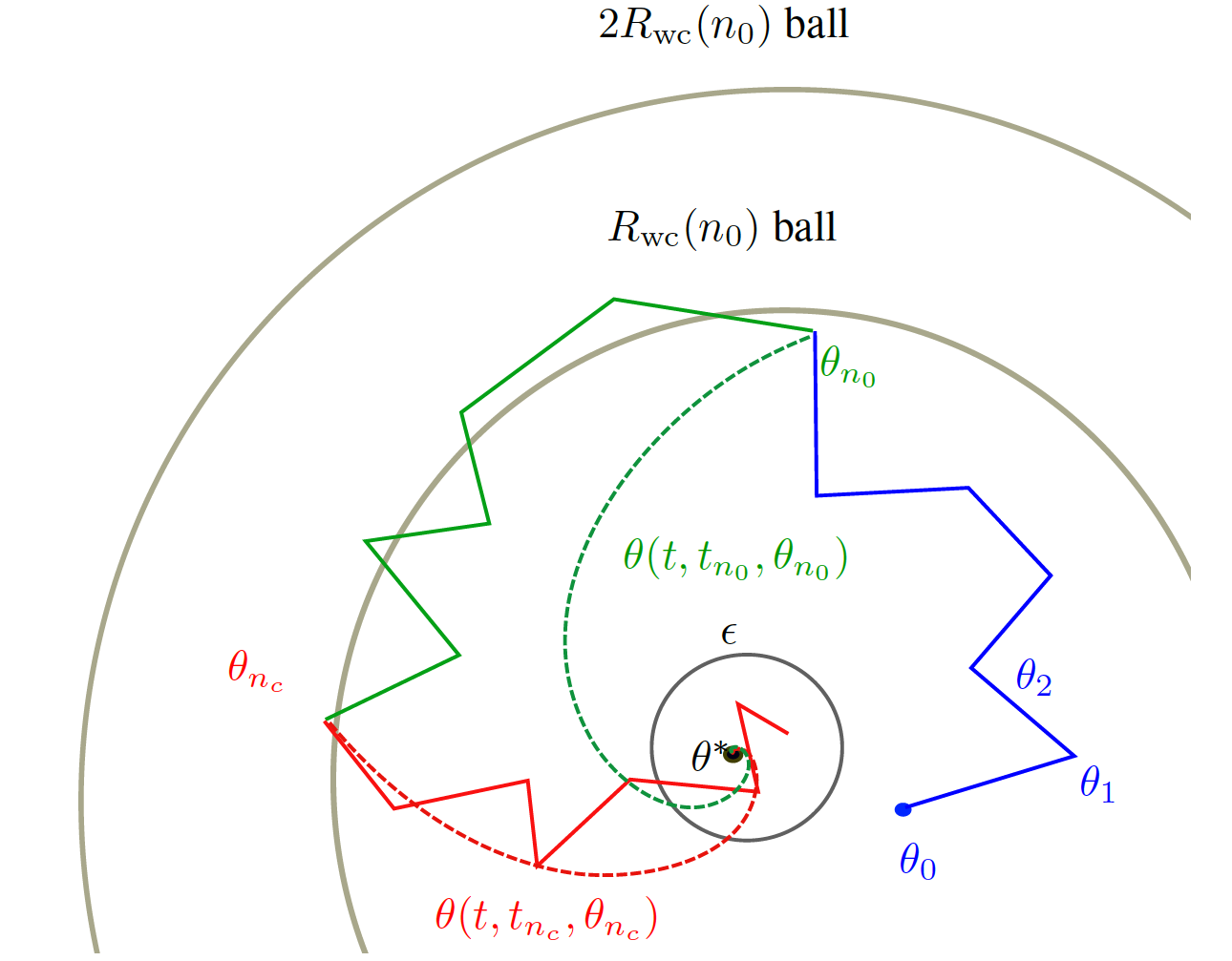
Figure 1: Visualization of the proof outline. The three balls (from large to small) are respectively the $2R_{\mathrm{wc}}(n_{0})$ ball, $R_{\mathrm{wc}}(n_{0})$ ball, and $\epsilon$ ball, where $R_{\mathrm{wc}}(n_{0})$ is from Lemma 5.4. The blue curve is the initial, possibly diverging phase of $\bar{\theta}(t)$. The green curve is $\bar{\theta}(t)$ when the stepsizes are moderate in size ($t_{n_{0}}\leq t\leq t_{n_{\textnormal{c}}}$ in the analysis). Similarly, the red curve is $\bar{\theta}(t)$ when the stepsizes are sufficiently small ($t>t_{n_{\textnormal{c}}}$). The dotted curves are the associated ODE trajectories $\theta(t,t_{n},\theta_{n})$.

Preliminaries

We establish some preliminary results here that will be used throughout this section. Let $s\in\mathbb{R},$ and $u_{0}\in\mathbb{R}^{d}.$ Using results from Chapter 6, (?), it follows that the solution $\theta(t,s,u_{0}),$ $t\geq s,$ of (13) satisfies the relation

$$\theta(t,s,u_{0})=\theta^{*}+e^{-A(t-s)}(u_{0}-\theta^{*})\enspace.$$ (15)

As the matrix $A$ is positive definite, for $\theta(t)\equiv\theta(t,s,u_{0}),$

$$\frac{d}{dt}\|\theta(t)-\theta^{*}\|^{2}=-2(\theta(t)-\theta^{*})^{\top}A(\theta(t)-\theta^{*})<0\enspace.$$

Hence

$$\|\theta(t^{\prime},s,u_{0})-\theta^{*}\|\leq\|\theta(t,s,u_{0})-\theta^{*}\|\enspace,$$ (16)

for all $t^{\prime}\geq t\geq s$ and $u_{0}.$

Let $\lambda$ be as in Theorem 3.5. From Corollary 3.6, p71, (?), $\exists K_{\lambda}\,\geq 1$ so that $\forall t\geq s$

$$\|e^{-A(t-s)}\|\leq K_{\lambda}\,e^{-\lambda(t-s)}\enspace.$$ (17)

Separately, as $t_{n+1}-t_{k+1}=\sum_{\ell=k+1}^{n}\alpha_{\ell}=\sum_{\ell=k+1}^{n}\tfrac{1}{\ell+1},$

$$\frac{(k+1)^{\lambda}}{(n+1)^{\lambda}}\leq e^{-\lambda(t_{n+1}-t_{k+1})}\leq\frac{(k+2)^{\lambda}}{(n+2)^{\lambda}}\enspace.$$ (18)

The following result is a consequence of $\boldsymbol{\mathcal{A}_{2}}$ that gives a bound directly on the martingale difference noise as a function of the iterates. We emphasize that this strong behavior of TD(0) is significant in our work. We also are not aware of other works that utilized it even though $\boldsymbol{\mathcal{A}_{2}}$ or equivalents are often assumed and accepted.

Lemma 5.1 (Martingale Noise Behavior).

For all $n\geq 0,$

$$\|M_{n+1}\|\leq K_{m}\,[1+\|\theta_{n}-\theta^{*}\|]\enspace,$$

where

$$K_{m}\,:=\frac{1}{4}\max\left\{2+[1+\gamma]\|A^{-1}\|\|b\|,1+\gamma+4\|A\|\right\}\enspace.$$

Remark 5.2.

The noise behavior usually used in the literature (e.g., (?; ?)) is the same as we assumed in $\boldsymbol{\mathcal{A}_{1}}$ for Theorem 3.1:

$$\mathbb{E}[||M_{n+1}||^{2}|{\cal F}_{n}]\leq K_{s}(1+||\theta_{n}||^{2})\enspace,$$

for some constant $K_{s}\geq 0$. However, here we assume the stronger $\boldsymbol{\mathcal{A}_{2}}$, which, using a similar proof technique to that of Lemma 5.1, implies

$$\||M_{n+1}||^{2}\leq 3[1+\gamma+\max(\|A\|,\|b\|)]^{2}(1+||\theta_{n}||^{2})$$

for all $n\geq 0.$

The remaining parts of the analysis rely on the comparison of the discrete TD(0) trajectory $\{\theta_{n}\}$ to the continuous solution $\theta(t)$ of the limiting ODE. For this, we first switch from directly treating $\{\theta_{n}\}$ to treating their linear interpolation $\{\bar{\theta}(t)\}$ as defined in (14). The key idea then is to use the VoP method (?) as in Lemma A.1, and express $\bar{\theta}(t)$ as a perturbation of $\theta(t)$ due to two factors: the discretization error and the martingale difference noise. Our quantification of these two factors is as follows. For the interval $[t_{\ell_{1}},t_{\ell_{2}}],$ let

$$E^{\text{d}}_{[\ell_{1},\ell_{2}]}:=\sum_{k=\ell_{1}}^{\ell_{2}-1}\int_{t_{k}}^{t_{k+1}}e^{-A(t_{n+1}-\tau)}A[\bar{\theta}(\tau)-\theta_{k}]\mathrm{d}\tau\enspace,$$

and

$$E^{\text{m}}_{[\ell_{1},\ell_{2}]}:=\sum_{k=\ell_{1}}^{\ell_{2}-1}\left[\int_{t_{k}}^{t_{k+1}}e^{-A(t_{n+1}-\tau)}\mathrm{d}\tau\right]M_{k+1}\enspace.$$

Corollary 5.3 (Comparison of SA Trajectory and ODE Solution).

For every $\ell_{2}\geq\ell_{1}$,

$$\bar{\theta}(t_{\ell_{2}})-\theta^{*}=\theta(t_{\ell_{2}},t_{\ell_{1}},\bar{\theta}(t_{\ell_{1}}))-\theta^{*}+E^{\text{d}}_{[\ell_{1},\ell_{2}]}+E^{\text{m}}_{[\ell_{1},\ell_{2}]}\enspace.$$

We highlight that both the paths, $\bar{\theta}(t)$ and $\theta(t,t_{\ell_{1}},\bar{\theta}(t_{\ell_{1}})),$ $t\geq t_{\ell_{1}},$ start at the same point $\bar{\theta}(t_{\ell_{1}})$ at time $t_{\ell_{1}}.$ Consequently, by bounding $E^{\text{d}}_{[\ell_{1},\ell_{2}]}$ and $E^{\text{m}}_{[\ell_{1},\ell_{2}]}$ we can estimate the distance of interest.

Part I – Initial Possible Divergence

In this section, we show that the TD(0) iterates lie in an $O(n)$-ball around $\theta^{*}.$ We stress that this is one of the results that enable us to accomplish more than existing literature. Previously, the distance of the initial iterates from $\theta^{*}$ was bounded using various assumptions, often justified with an artificial projection step which we are able to avoid.

Let $R_{0}:=1+\|\theta_{0}-\theta^{*}\|.$

Lemma 5.4 (Worst-case Iterates Bound).

For $n\geq 0,$

$$\|\theta_{n}-\theta^{*}\|\leq R_{\mathrm{wc}}(n)\enspace,$$

where

$$R_{\mathrm{wc}}(n):=[n+1]C_{*}R_{0}$$

and $C_{*}:=1+\|\theta^{*}\|\leq 1+\|A^{-1}\|\;\|b\|$

Next, since $\|M_{n+1}\|$ is linearly bounded by $\|\theta_{n}-\theta^{*}\|$, the following result shows that $\|M_{n+1}\|$ is $O(n)$ as well. It follows from Lemmas 5.1 and 5.4.

Corollary 5.5 (Worst-case Noise Bound).

For $n\geq 0,$

$$\|M_{n+1}\|\leq K_{m}\,[1+C_{*}R_{0}][n+1]\enspace.$$

Part II – Rate of Convergence

Here, we bound the probability of the event

$$\mathcal{E}(n_{0},n_{1}):=\{\|\theta_{n}-\theta^{*}\|\leq\epsilon\;\forall n>n_{0}+n_{1}\}\enspace$$

for sufficiently large $n_{0},n_{1};$ how large they should be will be elaborated later. We do this by comparing the TD(0) trajectory $\theta_{n}$ with the ODE solution $\theta(t_{n},t_{n_{0}},\bar{\theta}(t_{n_{0}}))$ $\forall n\geq n_{0}$; for this we will use Corollary  5.3 along with Lemma 5.4. Next, we show that if $n_{0}$ is sufficiently large, or equivalently the stepsizes $\{\alpha_{n}\}_{n\geq n_{0}}$ are small enough, then after waiting for a finite number of iterations from $n_{0},$ the TD(0) iterates are $\epsilon-$close to $\theta^{*}$ w.h.p. The sufficiently long waiting time ensures that the ODE solution $\theta(t_{n+1},t_{n_{0}},\bar{\theta}_{n_{0}})$ is $\epsilon-$close to $\theta^{*};$ the small stepsizes ensure that the discretization error and martingale difference noise are small enough.

Let $\delta\in(0,1),$ and let $\epsilon$ be such that $\epsilon>0.$ Also, for an event $\mathcal{E},$ let $\mathcal{E}^{c}$ denote its complement and let $\{\mathcal{E}_{1},\mathcal{E}_{2}\}$ denote $\mathcal{E}_{1}\cap\mathcal{E}_{2}.$ We begin with a careful decomposition of $\mathcal{E}^{c}(n_{0},n_{1}),$ the complement of the event of interest. The idea is to break it down into an incremental union of events. Each such event has an inductive structure: good up to iterate $n$ (denoted by $G_{n_{0},n}$ below) and the $(n+1)-$th iterate is bad. The good event $G_{n_{0},n}$ holds when all the iterates up to $n$ remain in an $O(n_{0})$ ball around $\theta^{*}.$ For $n<n_{0}+n_{1},$ the bad event means that $\theta_{n+1}$ is outside the $O(n_{0})$ ball around $\theta^{*},$ while for $n\geq n_{0}+n_{1},$ the bad event means that $\theta_{n+1}$ is outside the $\epsilon$ ball around $\theta^{*}.$ Formally, for $n_{1}\geq 1,$ define the events

$$\mathcal{E}_{n_{0},n_{1}}^{\textnormal{mid}}:=\bigcup_{n=n_{0}}^{n_{0}+n_{1}-1}\!\left\{G_{n_{0},n},\|\theta_{n+1}-\theta^{*}\|\!>\!2R_{\mathrm{wc}}(n_{0})\right\}\enspace,$$

$$\mathcal{E}_{n_{0},n_{1}}^{\textnormal{after}}$$ (19)

$$:=\bigcup_{n=n_{0}+n_{1}}^{\infty}\left\{G_{n_{0},n},\|\theta_{n+1}-\theta^{*}\|>\min\{\epsilon,2R_{\mathrm{wc}}(n_{0})\}\right\}\;,$$ (20)

and, $\forall n\geq n_{0},$ let

$$G_{n_{0},n}\!:=\!\left\{\bigcap_{k=n_{0}}^{n}\!\{\|\theta_{k}-\theta^{*}\|\!\leq\!2R_{\mathrm{wc}}(n_{0})\}\right\}\enspace.$$

Using the above definitions, the decomposition of $\mathcal{E}^{c}(n_{0},n_{1})$ is the following relation.

Lemma 5.6 (Decomposition of Event of Interest).

For $n_{0},n_{1}\geq 1,$

$$\mathcal{E}^{c}(n_{0},n_{1})\subseteq\mathcal{E}_{n_{0},n_{1}}^{\textnormal{mid}}\cup\mathcal{E}_{n_{0},n_{1}}^{\textnormal{after}}\enspace.$$

For the following results, define the constants

$$C_{m2}:=\begin{cases}\frac{6K_{m}\,K_{\lambda}\,2^{\lambda-0.5}}{\sqrt{2\lambda-1}}&\text{ if $\lambda>0.5$}\\ \frac{6K_{m}\,K_{\lambda}\,}{\sqrt{1-2\lambda}}&\text{ if $\lambda<0.5$ \enspace.}\end{cases}$$

Next, we show that on the “good” event $G_{n_{0},n},$ the discretization error is small for all sufficiently large $n.$

Lemma 5.7 (Part II Discretization Error Bound).

For any

$$n\geq n_{0}\geq\tfrac{K_{\lambda}6\|A\|(\|A\|+2K_{m}\,)}{\lambda},$$

$$\|E_{[n_{0},n+1]}^{d}\|\leq\tfrac{1}{3}[n_{0}+1]C_{*}R_{0}=\tfrac{1}{3}R_{\mathrm{wc}}(n_{0}).$$

Furthermore, for

$$n\geq n_{\textnormal{c}}\geq\left(1+\tfrac{K_{\lambda}6\|A\|(\|A\|+2K_{m}\,)C_{*}R_{0}}{\lambda\min\{\epsilon,R_{\mathrm{wc}}(n_{0})\}}\right)(n_{0}+1)$$

it thus also holds on $G_{n_{0},n}$ that

$$\|E_{[n_{\textnormal{c}},n+1]}^{d}\| \leq\tfrac{1}{3}\min\{\epsilon,[n_{0}+1]C_{*}R_{0}\}$$

$$=\tfrac{1}{3}\min\{\epsilon,R_{\mathrm{wc}}(n_{0})\}\enspace.$$

The next result gives a bound on the probability that, on the “good” event $G_{n_{0},n},$ the martingale difference noise is small when $n$ is large. The bound has two forms for the different values of $\lambda$.

Lemma 5.8 (Part II Martingale Difference Noise Concentration).

Let $n_{0}\geq 1$ and $R\geq 0.$ Let $n\geq n^{\prime}\geq n_{0}.$

• For $\lambda>1/2,$

  $$\Pr\{G_{n_{0},n}, \|E_{[n^{\prime},n+1]}^{m}\|\geq R\}$$

  $$\leq 2d^{2}\exp\left[-\frac{(n+1)R^{2}}{2d^{3}C_{m2}^{2}R_{\mathrm{wc}}^{2}(n_{0})}\right]\enspace.$$

• For $\lambda<1/2,$

  $$\Pr\{G_{n_{0},n}, \|E_{[n^{\prime},n+1]}^{m}\|\geq R\}$$

  $$\leq 2d^{2}\exp\left[-\frac{[n^{\prime}+1]^{1-2\lambda}(n+1)^{2\lambda}R^{2}}{2d^{3}C_{m2}^{2}R_{\mathrm{wc}}^{2}(n_{0})}\right]\enspace.$$

Having Lemma 5.7, we substitute $R=\tfrac{R_{\mathrm{wc}}(n_{0})}{2}$ in Lemma 5.8 and estimate the resulting sum to bound $\mathcal{E}_{n_{0},n_{1}}^{\textnormal{mid}}$.

Lemma 5.9 (Bound on Probability of $\mathcal{E}_{n_{0},n_{1}}^{\textnormal{mid}}$).

Let $n_{0}\geq\max\left\{\tfrac{K_{\lambda}6\|A\|(\|A\|+2K_{m}\,)}{\lambda},2^{\frac{1}{\lambda}}\right\}$ and $n_{1}\geq 1.$

• For $\lambda>1/2,$

  $$\Pr\{\mathcal{E}_{n_{0},n_{1}}^{\textnormal{mid}}\}\leq 16d^{5}C_{m2}^{2}\exp\left[-\frac{n_{0}}{8d^{3}C_{m2}^{2}}\right]\enspace.$$

• For $\lambda<1/2,$

  $$\Pr\{\mathcal{E}_{n_{0},n_{1}}^{\textnormal{mid}}\}\leq\\ 2d^{2}\left[\frac{8d^{3}C_{m2}^{2}}{\lambda}\right]^{\frac{1}{2\lambda}}\frac{\exp[-\frac{n_{0}}{64d^{3}C_{m2}^{2}}]}{(n_{0}+1)^{\frac{1-2\lambda}{2\lambda}}}\enspace.$$

Lastly, we upper bound $\mathcal{E}_{n_{0},n_{1}}^{\textnormal{after}}$ in the same spirit as $\mathcal{E}_{n_{0},n_{1}}^{\textnormal{mid}}$ in Lemma 5.9, again using Lemmas 5.7 and 5.8; this time with $R=\frac{\epsilon}{3}$ .

Lemma 5.10 (Bound on Probability of $\mathcal{E}_{n_{0},n_{1}}^{\textnormal{after}}$).

Let

$$n_{0}\geq\max\left\{\tfrac{K_{\lambda}6\|A\|(\|A\|+2K_{m}\,)}{\lambda},2^{\frac{1}{\lambda}}\right\}$$

and

$$n_{\textnormal{c}}\geq\left(1+\tfrac{K_{\lambda}6\|A\|(\|A\|+2K_{m}\,)}{\lambda\min\{\epsilon,R_{\mathrm{wc}}(n_{0})\}}\right)R_{\mathrm{wc}}(n_{0}).$$

Let $n_{1}\equiv n_{1}(\epsilon,n_{\textnormal{c}},n_{0})\geq(n_{\textnormal{c}}+1)\left[\frac{6K_{\lambda}\,R_{\mathrm{wc}}(n_{0})}{\epsilon}\right]^{1/\lambda}-n_{0}.$

• For $\lambda>1/2,$

  $$\Pr\{ \mathcal{E}_{n_{0},n_{1}}^{\textnormal{after}}\}\leq 36d^{5}C_{m2}^{2}\left[\frac{R_{\mathrm{wc}}(n_{0})}{\epsilon}\right]^{2}$$

  $$\times\exp\left[-\frac{(6K_{\lambda}\,)^{1/\lambda}}{18d^{3}C_{m2}^{2}}(n_{\textnormal{c}}+1)\left[\frac{\epsilon}{R_{\mathrm{wc}}(n_{0})}\right]^{2-\tfrac{1}{\lambda}}\right].$$

• For $\lambda<1/2,$

  $$\Pr\{\mathcal{E}_{n_{0},n_{1}}^{\textnormal{after}}\}\leq 2d^{2} \left[\frac{18d^{3}C_{m2}^{2}[R_{\mathrm{wc}}(n_{0})]^{2}}{\epsilon^{2}\lambda}\right]^{\frac{1}{2\lambda}}$$

  $$\times\exp\left[-\frac{K_{\lambda}^{2}}{4d^{3}C_{m2}^{2}}(n_{\textnormal{c}}+1)\right].$$

We are now ready to put the pieces together for proving Theorem 3.5. For the detailed calculations see end of Appendix B.

Proof of Theorem 3.5.

From Lemma 5.6, by a union bound,

$$\Pr\{\mathcal{E}^{c}(n_{0},n_{1})\}\leq\Pr\{\mathcal{E}_{n_{0},n_{1}}^{\textnormal{mid}}\}+\Pr\{\mathcal{E}_{n_{0},n_{1}}^{\textnormal{after}}\}\enspace.$$

The behavior of $\mathcal{E}_{n_{0},n_{1}}^{\textnormal{mid}}$ is dictated by $n_{0}$, while the behavior of $\mathcal{E}_{n_{0},n_{1}}^{\textnormal{after}}$ by $n_{1}$. Using Lemma 5.9, we set $n_{0}$ so that $\mathcal{E}_{n_{0},n_{1}}^{\textnormal{mid}}$ is less than $\delta/2$, resulting in the condition $n_{0}=O\left(\ln\tfrac{1}{\delta}\right)$. Next, using Lemma 5.10, we set $n_{1}$ so that $\mathcal{E}_{n_{0},n_{1}}^{\textnormal{after}}$ is less than $\delta/2$, resulting in

$$n_{1}=\tilde{O}\left(\big{[}{(1/\epsilon)}\ln{(1/\delta)}\big{]}^{\max\left\{1+{1/\lambda},2\right\}}\right)$$

for $\lambda>1/2,$ and

$$n_{1}=\tilde{O}\left(\big{[}{(1/\epsilon)}\ln{(1/\delta)}\big{]}^{1+{1/\lambda}}\right)$$

for $\lambda<1/2.$ ∎

6 Discussion

In this work, we obtained the first convergence rate estimates for an unaltered version of the celebrated TD(0). It is, in fact, the first to show rates of an unaltered online TD algorithm of any type.

As can be seen from Theorem 3.5, the bound explodes when the matrix $A$ is ill-conditioned. We stress that this is not an artifact of the bound but an inherent property of the algorithm itself. This happens because along the eigenspace corresponding to the zero eigenvalues, the limiting ODE makes no progress and consequently no guarantees for the (noisy) TD(0) method can be given in this eigenspace. As is well known, the ODE will, however, advance in the eigenspace corresponding to the non-zero eigenvalues to a solution which we refer to as the truncated solution. Given this, one might expect that the (noisy) TD(0) method may also converge to this truncated solution. We now provide a short example that suggests that this is in fact not the case. Let

$$A:=\begin{bmatrix}1&1\\ 0&0\end{bmatrix},\text{ and }b:=\begin{bmatrix}2\\ 0\end{bmatrix}.$$

Clearly, $\theta^{*}:=\begin{bmatrix}1&1\end{bmatrix}^{\top}$ is a vector satisfying $b=A\theta^{*}$ and the eigenvalues of $A$ are $1$ and $0.$ Consider the update rule $\theta_{n+1}=\theta_{n}+\alpha_{n}[b-A\theta_{n}+M_{n+1}]$ with

$$M_{n+1}=\begin{bmatrix}1\\ 1\end{bmatrix}Z_{n+1}[\theta_{n}(2)-\theta^{*}(2)].$$

Here $v(i)$ is the $i-$th coordinate of vector $v,$ and $\{Z_{n}\}$ are IID Bernoulli $\{-1,+1\}$ random variables. For an initial value $\theta_{0},$ one can see that the (unperturbed) ODE for the above update rule converges to $\begin{bmatrix}-1&1\end{bmatrix}^{\top}\theta_{0}(2)+b;$ this is not $\theta^{*},$ but the truncated solution mentioned above. For the same initial point, predicting the behavior of the noisy update is not easy. Rudimentary simulations show the following. In the initial phase (when the stepsizes are large) the noise dictates how the iterates behave. Afterwards, at a certain stage when the stepsizes become sufficiently small, an “effective $\theta_{0}$” is detected, from which the iterates start converging to a new truncated solution, corresponding to this “effective $\theta_{0}$”. This new truncated solution is different per each run and is often very different from the truncated solution corresponding the initial iterate $\theta_{0}.$

Separately, we stress that our proof technique is general and can be used to provide convergence rates for TD with non-linear function approximations, such as neural networks. Specifically, this can be done using the non-linear analysis presented in (?). There, the more general form of Variation of Parameters is used: the so-called Alekseev’s formula. However, as mentioned in Section 1, the caveat there is that the $n_{0}-$th iterate needs to be in the domain of attraction of the desired asymptotically stable equilibrium point. Nonetheless, we believe that one should be able to extend our present approach to non-linear ODEs with a unique global equilibrium point. For non-linear ODEs with multiple stable points, the following approach can be considered. In the initial phase, the location of the SA iterates is a Markov chain with the state space being the domain of attraction associated with different attractors (?). Once the stepsizes are sufficiently small, analysis as in our current paper via Alekseev’s formula may enable one to obtain expectation and high probability convergence rate estimates. In a similar fashion, one may obtain such estimates even for the two timescale setup by combining the ideas here with the analysis provided in (?).

Finally, future work can extend to a more general family learning rates, including the commonly used adaptive ones. Building upon Remark 5.2, we believe that a stronger expectation bound may hold for TD(0) with uniformly bounded features and rewards. This may enable obtaining tighter convergence rate estimates for TD(0) even with generic stepsizes.

7 Acknowledgments

This research was supported by the European Community’s Seventh Framework Programme (FP7/2007-2013) under grant agreement 306638 (SUPREL). A portion of this work was completed when Balazs Szorenyi and Gugan Thoppe were postdocs at Technion, Israel. Gugan’s research was initially supported by ERC grant 320422 and is now supported by grants NSF IIS-1546331, NSF DMS-1418261, and NSF DMS-1613261.

Appendix A Variation of Parameters Formula

Let $\theta(t,s,\bar{\theta}(s)),$ $t\geq s,$ be the solution to (13) starting at $\bar{\theta}(s)$ at time $t=s.$ For $k\geq 0,$ and $\tau\in[t_{k},t_{k+1}),$ let

$$\zeta_{1}(\tau):=h(\theta_{k})-h(\bar{\theta}(\tau))=A[\bar{\theta}(\tau)-\theta_{k}]$$ (21)

and

$$\zeta_{2}(\tau):=M_{k+1}\enspace.$$ (22)

Lemma A.1.

Let $i\geq 0.$ For $t\geq t_{i}.$

$$\bar{\theta}(t)=\theta(t,t_{i},\bar{\theta}(t_{i}))+\int_{t_{i}}^{t}e^{-A(t-\tau)}[\zeta_{1}(\tau)+\zeta_{2}(\tau)]\mathrm{d}\tau.$$

Proof.

For $n\geq 0$ and $t\in[t_{n},t_{n+1}),$ by simple algebra,

$$\bar{\theta}(t)-\bar{\theta}(t_{i})=\frac{t-t_{n}}{\alpha_{n}}[\theta_{n+1}-\theta_{n}]+\sum_{k=i}^{n-1}[\theta_{k+1}-\theta_{k}].$$

Combining this with (2), (21), and (22), and using the relations $\tau-t_{n}=\int_{t_{n}}^{t}\mathrm{d}\tau$ and $\alpha_{k}=\int_{t_{k}}^{t_{k+1}}\mathrm{d}\tau,$ we have

$$\bar{\theta}(t)=\bar{\theta}(t_{i})+\int_{t_{i}}^{t}h(\bar{\theta}(\tau))\mathrm{d}\tau+\int_{t_{i}}^{t}[\zeta_{1}(\tau)+\zeta_{2}(\tau)]\mathrm{d}\tau.$$

Separately, writing (13) in integral form, we have

$$\theta(t,t_{i},\bar{\theta}(t_{i}))=\bar{\theta}(t_{i})+\int_{t_{i}}^{t}h(\theta(\tau))\mathrm{d}\tau.$$

From the above two relations and the VoP formula (?), the desired result follows. ∎

Appendix B Supplementary Material for Proof of Theorem 3.5

Proof of Lemma 5.1.

We have

$$\|M_{n+1}\| = \|r_{n}\phi_{n}+(\gamma\phi_{n}^{\prime}-\phi_{n})^{\top}\theta_{n}\phi_{n}-[b-A\theta_{n}]\|$$

$$= \|r_{n}\phi_{n}+(\gamma\phi_{n}^{\prime}-\phi_{n})^{\top}(\theta_{n}-\theta^{*})\phi_{n}$$

$$\quad+(\gamma\phi_{n}^{\prime}-\phi_{n})^{\top}\theta^{*}\phi_{n}+A(\theta_{n}-\theta^{*})\|$$

$$\leq \frac{1}{2}+\frac{[1+\gamma]}{4}\|A^{-1}\|\;\|b\|+\frac{[1+\gamma+4\|A\|]}{4}\|\theta_{n}-\theta^{*}\|,$$

where the first relation follows from (3), the second holds as $b=A\theta^{*},$ while the third follows since $\boldsymbol{\mathcal{A}_{2}}$ holds and $\theta^{*}=A^{-1}b.$ The desired result is now easy to see. ∎

Proof of Corollary 5.3.

The result follows by using Lemma A.1 from Appendix A, with $i=\ell_{1},$ $t=t_{\ell_{2}},$ and subtracting $\theta^{*}$ from both sides. ∎

Proof of Lemma 5.4.

The proof is by induction. The claim holds trivially for $n=0.$ Assume the claim for $n.$ Then from (1),

$$\|\theta_{n+1}-\theta^{*}\|\leq\|\theta_{n}-\theta^{*}\|+\alpha_{n}\|[\gamma\phi_{n}^{\prime}-\phi_{n}]^{\top}\theta^{*}\phi_{n}\|+\alpha_{n}\|r_{n}\phi_{n}\|+\alpha_{n}\|[\gamma\phi_{n}^{\prime}-\phi_{n}]^{\top}[\theta_{n}-\theta^{*}]\phi_{n}\|\enspace.$$

Applying the Cauchy-Schwarz inequality, and using $\boldsymbol{\mathcal{A}_{2}}$ and the fact that $\gamma\leq 1,$ we have

$$\|\theta_{n+1}-\theta^{*}\|\leq\|\theta_{n}-\theta^{*}\|+\frac{\alpha_{n}}{2}C_{*}+\frac{\alpha_{n}}{2}\|\theta_{n}-\theta^{*}\|.$$

Now as $1\leq R_{0},$ we have

$$\|\theta_{n+1}-\theta^{*}\|\leq\left[1+\frac{\alpha_{n}}{2}\right]\|\theta_{n}-\theta^{*}\|+\frac{\alpha_{n}}{2}C_{*}R_{0}.$$

Using the induction hypothesis and the stepsize choice, the claim for $n+1$ is now easy to see. The desired result thus follows. ∎

Proof of Lemma 5.6.

For any two events $\mathcal{E}_{1}$ and $\mathcal{E}_{2},$ note that

$$\mathcal{E}_{1}=[\mathcal{E}_{2}^{c}\cap\mathcal{E}_{1}]\cup[\mathcal{E}_{2}\cap\mathcal{E}_{1}]\subseteq\mathcal{E}_{2}^{c}\cup[\mathcal{E}_{2}\cap\mathcal{E}_{1}]\enspace.$$ (23)

Separately, for any sequence of events $\{\mathcal{E}_{k}\},$ observe that

$$\bigcup_{k=1}^{m}\mathcal{E}_{k}=\left[\bigcup_{k=1}^{m}\left(\left[\bigcup_{i=1}^{k-1}\mathcal{E}_{i}\right]^{c}\cap\mathcal{E}_{k}\right)\right]\enspace,$$ (24)

where $\bigcup_{i=i_{1}}^{i_{2}}\mathcal{E}_{i}=\emptyset$ whenever $i_{1}>i_{2}.$ Using (23), we have

$$\mathcal{E}^{c}(n_{0},n_{1})\subseteq G_{n_{0},n_{0}+n_{1}}^{c}\cup[G_{n_{0},n_{0}+n_{1}}\cap\mathcal{E}^{c}(n_{0},n_{1})]\enspace.$$ (25)

From Lemma 5.4, $\{\|\theta_{n_{0}}-\theta^{*}\|\leq R_{\mathrm{wc}}(n_{0})\}$ is a certain event. Hence it follows from (24) that

$$G_{n_{0},n_{0}+n_{1}}^{c}=\mathcal{E}_{n_{0},n_{1}}^{\textnormal{mid}}.$$ (26)

Similarly, from (24) and the fact that $\epsilon\leq R_{0},$

$$G_{n_{0},n_{0}+n_{1}}\cap\mathcal{E}^{c}(n_{0},n_{1})\subseteq\mathcal{E}_{n_{0},n_{1}}^{\textnormal{after}}\enspace.$$ (27)

Substituting (26) and (27) in (25) gives

$$\mathcal{E}^{c}(n_{0},n_{1})\subseteq\mathcal{E}_{n_{0},n_{1}}^{\textnormal{mid}}\cup\mathcal{E}_{n_{0},n_{1}}^{\textnormal{after}}\enspace.$$

The claimed result follows. ∎

Proof of Lemma 5.7.

For $n\geq n^{\prime}\geq n_{0}\geq 0$, by its definition and the triangle inequality,

$$\|E^{\text{d}}_{[n^{\prime},n+1]}\|\!\leq\!\sum_{k=n^{\prime}}^{n}\!\!\int_{t_{k}}^{t_{k+1}}\|e^{-A(t_{n+1}\!-\tau)}\|\|A\|\|\bar{\theta}(\tau)-\theta_{k}\|\mathrm{d}\tau.$$

Fix a $k\in\{n^{\prime},\ldots,n\}$ and $\tau\in[t_{k},t_{k+1}).$ Then using (14), (2), (4), and the fact that $(\tau-t_{k})\leq\alpha_{k},$ we have

$$\|\bar{\theta}(\tau)-\theta_{k}\|\leq\alpha_{k}[\|A\|\|\theta_{k}-\theta^{*}\|+\|M_{k+1}\|]\enspace.$$

Combining this with Lemma 5.1, we get

$$\|\bar{\theta}(\tau)-\theta_{k}\|\leq\alpha_{k}[K_{m}\,+(\|A\|+K_{m}\,)\|\theta_{k}-\theta^{*}\|]\enspace.$$

As the event $G_{n_{0},n}$ holds, and since $\alpha_{k}\leq\alpha_{n^{\prime}}$ and $R_{\mathrm{wc}}(n_{0})\geq 1,$ we have

$$\|\bar{\theta}(\tau)-\theta_{k}\|\leq 2[\|A\|+2K_{m}\,]\alpha_{n^{\prime}}[n_{0}+1]C_{*}R_{0}\enspace.$$

From the above discussion, (17), the stepsize choice, and the facts that

$$\sum_{k=n^{\prime}}^{n}\int_{t_{k}}^{t_{k+1}}e^{-\lambda(t_{n+1}-\tau)}\mathrm{d}\tau=\int_{t_{n^{\prime}}}^{t_{n+1}}e^{-\lambda(t_{n+1}-\tau)}\mathrm{d}\tau\leq\frac{1}{\lambda}\enspace,$$

and $\alpha_{k}\leq\alpha_{n^{\prime}}\leq\alpha_{n_{0}},$ we get

$$\|E^{\text{d}}_{[n^{\prime},n+1]}\|\leq\tfrac{K_{\lambda}2\|A\|(\|A\|+2K_{m}\,)(n_{0}+1)C_{*}R_{0}}{\lambda(n^{\prime}+1)}\enspace.$$

The desired results now follow by substituting $n^{\prime}$ first with $n_{0}$ and then with $n_{c}.$ ∎

Proof of Lemma 5.8.

Let $Q_{k,n}=\int_{t_{k}}^{t_{k+1}}e^{-A(t_{n+1}-\tau)}\mathrm{d}\tau.$ Then, for any $n_{0}\leq n^{\prime}\leq n,$

$$E_{[n^{\prime},n+1]}^{m}=\sum_{k=n^{\prime}}^{n}Q_{k,n}M_{k+1}\enspace,$$

a sum of martingale differences. When the event $G_{n_{0},n}$ holds, it follows that the indicator $1_{G_{n_{0},k}}=1$ $\forall k\in\{n_{0},\ldots,n^{\prime},\ldots n\}.$ Hence, for any $R\geq 0,$

$$\Pr\{G_{n_{0},n},\|E_{[n^{\prime},n+1]}^{m}\|\geq R\} = \Pr\left\{G_{n_{0},n},\left\|\sum_{k=n^{\prime}}^{n}Q_{k,n}M_{k+1}1_{G_{n_{0},k}}\right\|\geq R\right\}$$

$$\leq \Pr\left\{\left\|\sum_{k=n^{\prime}}^{n}Q_{k,n}M_{k+1}1_{G_{n_{0},k}}\right\|\geq R\right\}.$$

Let $Q^{ij}_{k,n}$ be the $i,j-$th entry of the matrix $Q_{k,n}$ and let $M_{k+1}^{j}$ be the $j-$th coordinate of $M_{k+1}.$ Then using the union bound twice on the above relation, we have

$$\Pr\{G_{n_{0},n},\|E_{[n^{\prime},n+1]}^{m}\|\geq R\}\leq\sum_{i=1}^{d}\sum_{j=1}^{d}\Pr\left\{\left|\sum_{k=n^{\prime}}^{n}Q^{ij}_{k,n}M^{j}_{k+1}1_{G_{n_{0},k}}\right|\geq\frac{R}{d\sqrt{d}}\right\}.$$

As $|Q_{k,n}^{ij}M_{k+1}^{j}|1_{G_{n_{0},k}}\leq\|Q_{k,n}\|\|M_{k+1}\|1_{G_{n_{0},k}}=:\beta_{k,n},$ Azuma-Hoeffding inequality now gives

$$\Pr\{G_{n_{0},n},\|E_{[n^{\prime},n+1]}^{m}\|\geq R\}\leq 2d^{2}\exp\left[-\frac{R^{2}}{2d^{3}\sum_{k=n^{\prime}}^{n}\beta_{k,n}^{2}}\right]\enspace.$$ (28)

On the event $G_{n_{0},k},$ $\|\theta_{k}-\theta^{*}\|\leq 2R_{\mathrm{wc}}(n_{0})$ by definition. Hence from Lemma 5.1, we have

$$\|M_{k+1}\|1_{G_{k}}\leq 3K_{m}\,R_{\mathrm{wc}}(n_{0})\enspace.$$ (29)

Also from (17), $\|Q_{k,n}\|\leq K_{\lambda}\,e^{-\lambda(t_{n+1}-t_{k+1})}\alpha_{k}.$ Combining the two inequalities, and using (18) along with the fact that $1/(k+1)\leq 2/(k+2),$ we get

$$\beta_{k,n} \leq 3K_{m}\,K_{\lambda}\,R_{\mathrm{wc}}(n_{0})e^{-\lambda(t_{n+1}-t_{k+1})}\alpha_{k}$$

$$\leq 6K_{m}\,K_{\lambda}\,R_{\mathrm{wc}}(n_{0})\frac{(k+2)^{\lambda-1}}{(n+2)^{\lambda}}\enspace.$$

Consider the case $\lambda>1/2.$ By treating the sum as a right Riemann sum, we have

$$\sum_{k=n^{\prime}}^{n}(k+2)^{2\lambda-2}\leq(n+3)^{2\lambda-1}/(2\lambda-1)\enspace.$$

As $(n+3)\leq 2(n+2)$ and $(n+2)\geq(n+1),$ we have

$$\sum_{k=n^{\prime}}^{n}\beta_{k,n}^{2}\leq C_{m2}^{2}\frac{R_{\mathrm{wc}}^{2}(n_{0})}{n+1}\enspace.$$

Now consider the case $\lambda<1/2.$ Again treating the sum as a right Riemann sum, we have

$$\sum_{k=n^{\prime}}^{n}(k+2)^{2\lambda-2}\leq\frac{1}{(1-2\lambda)[n^{\prime}+1]^{1-2\lambda}}\enspace.$$

As $(n+2)\geq(n+1),$ it follows that

$$\sum_{k=n^{\prime}}^{n}\beta_{k,n}^{2}\leq C_{m2}^{2}\frac{R_{\mathrm{wc}}^{2}(n_{0})}{[n^{\prime}+1]^{1-2\lambda}(n+1)^{2\lambda}}\enspace.$$

Substituting $\sum_{k=n_{0}}^{n}\beta_{k,n}^{2}$ bounds in (28), the desired result is easy to see. ∎

Conditional Results on the Bad Events

On the first “bad” event $\mathcal{E}_{n_{0},n_{1}}^{\textnormal{mid}},$ the TD(0) iterate $\theta_{n}$ for at least one $n$ between $n_{0}+1$ and $n_{0}+n_{1}$ leaves the $2R_{\mathrm{wc}}(n_{0})$ ball around $\theta^{*}.$ Lemma 5.9 shows that this event has low probability. Its proof is the following.

Proof of Lemma 5.9.

From Corollary 5.3, we have

$$\|\theta_{n+1}-\theta^{*}\|\leq\|\theta(t_{n+1},t_{n_{0}},\theta_{n_{0}})-\theta^{*}\|+\|E^{\text{d}}_{[n_{0},n+1]}\|+\|E^{\text{m}}_{[n_{0},n+1]}\|\enspace.$$

Suppose the event $G_{n_{0},n}$ holds. Then from (16),

$$\|\theta(t_{n+1},t_{n_{0}},\theta_{n_{0}})-\theta^{*}\|\leq\|\theta_{n_{0}}-\theta^{*}\|\leq R_{\mathrm{wc}}(n_{0})\enspace.$$

Also, as $n_{0}\geq\tfrac{K_{\lambda}6\|A\|(\|A\|+2K_{m}\,)}{\lambda}$, by Lemma 5.7, $\|E^{\text{d}}_{[n_{0},n+1]}\|\leq R_{\mathrm{wc}}(n_{0})/3.$ From all of the above, we have

$$\{G_{n_{0},n},\|\theta_{n+1}-\theta^{*}\|>2R_{\mathrm{wc}}(n_{0})\}\subseteq\{G_{n_{0},n},\|E^{\text{m}}_{[n_{0},n+1]}\|>R_{\mathrm{wc}}(n_{0})/2\}\enspace.$$

From this, we get

$$\mathcal{E}_{n_{0},n_{1}}^{\textnormal{mid}}\subseteq \bigcup_{n=n_{0}}^{n_{0}+n_{1}-1}\!\left\{G_{n_{0},n},\|E^{\text{m}}_{[n_{0},n+1]}\|>\tfrac{R_{\mathrm{wc}}(n_{0})}{2}\right\}$$

$$\subseteq \bigcup_{n=n_{0}}^{\infty}\!\left\{G_{n_{0},n},\|E^{\text{m}}_{[n_{0},n+1]}\|>\tfrac{R_{\mathrm{wc}}(n_{0})}{2}\right\}\enspace.$$

Consequently,

$$\Pr\{\mathcal{E}_{n_{0},n_{1}}^{\textnormal{mid}}\}\leq\\ \sum_{n=n_{0}}^{\infty}\!\!\Pr\!\left\{G_{n_{0},n},\|E^{\text{m}}_{[n_{0},n+1]}\|\!>\!\tfrac{R_{\mathrm{wc}}(n_{0})}{2}\right\}.$$ (30)

Consider the case $\lambda>1/2.$ Lemma 5.8 shows that

$$\Pr\left\{G_{n_{0},n},\|E^{\text{m}}_{[n_{0},n+1]}\|>\tfrac{R_{\mathrm{wc}}(n_{0})}{2}\right\}\leq 2d^{2}\exp\left[-\frac{n+1}{8d^{3}C_{m2}^{2}}\right]\enspace.$$

Substituting this in (30) and treating the resulting expression as a right Riemann sum, the desired result is easy to see.

Now consider the case $\lambda<1/2.$ From Lemma 5.8, we get

$$\Pr\left\{G_{n_{0},n},\|E^{\text{m}}_{[n_{0},n+1]}\|>\tfrac{R_{\mathrm{wc}}(n_{0})}{2}\right\}\leq 2d^{2}\exp\left[-\frac{(n_{0}+1)^{1-2\lambda}(n+1)^{2\lambda}}{8d^{3}C_{m2}^{2}}\right]\enspace.$$

Let $\ell_{n_{0}}:=(n_{0}+1)^{1-2\lambda}/8d^{3}C_{m2}^{2}.$ Observe that

$$\sum_{n=n_{0}}^{\infty}\exp[-\ell_{n_{0}}(n+1)^{2\lambda}]$$

$$\leq\sum_{i=\lfloor(n_{0}+1)^{2\lambda}\rfloor}^{\infty}e^{-i\ell_{n_{0}}}|\{n:\lfloor(n+1)^{{2\lambda}}\rfloor=i\}|$$

$$\leq\frac{1}{2\lambda}\sum_{i=\lfloor(n_{0}+1)^{2\lambda}\rfloor}^{\infty}e^{-i\ell_{n_{0}}}\;(i+1)^{\frac{1-{2\lambda}}{{2\lambda}}}$$ (31)

$$\leq\frac{1}{{2\lambda}}\sum_{i=\lfloor(n_{0}+1)^{2\lambda}\rfloor}^{\infty}e^{-i\ell_{n_{0}}/2}e^{-i\ell_{n_{0}}/2}\;(i+1)^{\frac{1-{2\lambda}}{{2\lambda}}}$$

$$\leq\frac{1}{{2\lambda}}\left[\frac{(1-{2\lambda})}{\ell_{n_{0}}{\lambda}}\right]^{\frac{1-{2\lambda}}{{2\lambda}}}\!\!e^{\frac{1}{2}[\ell_{n_{0}}-\frac{1-2\lambda}{\lambda}]}\sum_{i=\lfloor(n_{0}+1)^{2\lambda}\rfloor}^{\infty}\!\!e^{-i\ell_{n_{0}}/2}$$ (32)

$$\leq\frac{1}{{\ell_{n_{0}}\lambda}}\left[\frac{(1-{2\lambda})}{\ell_{n_{0}}{\lambda}}\right]^{\frac{1-{2\lambda}}{{2\lambda}}}\!\!e^{\frac{1}{2}[\ell_{n_{0}}-\frac{1-2\lambda}{\lambda}]}e^{-\frac{\ell_{n_{0}}{n_{0}}^{2\lambda}}{4}}$$ (33)

$$\leq\left[\frac{1-2\lambda}{e}\right]^{\frac{1-2\lambda}{2\lambda}}\left[\frac{8d^{3}C_{m2}^{2}}{\lambda}\right]^{\frac{1}{2\lambda}}\frac{\exp[-\frac{n_{0}}{64d^{3}C_{m2}^{2}}]}{(n_{0}+1)^{\frac{1-2\lambda}{2\lambda}}}\enspace$$ (34)

$$\leq\left[\frac{8d^{3}C_{m2}^{2}}{\lambda}\right]^{\frac{1}{2\lambda}}\frac{\exp[-\frac{n_{0}}{64d^{3}C_{m2}^{2}}]}{(n_{0}+1)^{\frac{1-2\lambda}{2\lambda}}}\enspace.$$ (35)

The relation (31) follows, as by calculus,

$$|\{n:\lfloor(n+1)^{{2\lambda}}\rfloor=i\}|\leq\frac{1}{2\lambda}(i+1)^{\frac{1-{2\lambda}}{{2\lambda}}}\enspace,$$

(32) holds since, again by calculus,

$$\max_{i\geq 0}e^{-i\ell_{n_{0}}/2}(i+1)^{\frac{1-2\lambda}{2\lambda}}\!\leq\!\left[\frac{(1-{2\lambda})}{\ell_{n_{0}}{\lambda}}\right]^{\frac{1-{2\lambda}}{{2\lambda}}}\!\!\!e^{\frac{1}{2}[\ell_{n_{0}}-\frac{1-2\lambda}{\lambda}]}\enspace,$$

(33) follows by treating the sum as a right Riemann sum, (34) follows by substituting the value of $\ell_{n_{0}}$ and using the fact that $n_{0}^{2\lambda}\geq 4$ and (35) holds since $1-2\lambda\leq 1.$ Substituting (35) in (30), the desired result follows. ∎

On the second “bad” event $\mathcal{E}_{n_{0},n_{1}}^{\textnormal{after}},$ the TD(0) iterate $\theta_{n}$ for at least one $n>n_{0}+n_{1}$ lies outside the $\min\{\epsilon,2R_{\mathrm{wc}}(n_{0})\}$ radius ball around $\theta^{*}.$ Lemma 5.10 shows that this event also has low probability.

Proof of Lemma 5.10.

Assume the event $G_{n_{0},n}$ holds for some $n\geq n_{\textnormal{c}}$. Then

$$\|\theta_{n_{\textnormal{c}}}-\theta^{*}\|\leq 2R_{\mathrm{wc}}(n_{0}).$$

Hence from (15) and (17), for $t\geq t_{n_{\textnormal{c}}},$ we have

$$\|\theta(t,t_{n_{\textnormal{c}}},\theta_{n_{\textnormal{c}}})-\theta^{*}\|\leq K_{\lambda}\,e^{-\lambda(t-t_{n_{\textnormal{c}}})}2R_{\mathrm{wc}}(n_{0})\enspace.$$ (36)

Now as $n_{1}\geq(n_{\textnormal{c}}+1)\left[\frac{6K_{\lambda}\,R_{\mathrm{wc}}(n_{0})}{\epsilon}\right]^{1/\lambda}-n_{0},$ it follows that $\forall n\geq n_{0}+n_{1},$

$$\|\theta(t_{n+1},t_{n_{\textnormal{c}}},\theta_{n_{\textnormal{c}}})-\theta^{*}\|\leq\frac{\epsilon}{3}\enspace.$$

Also, as $n_{\textnormal{c}}\geq\left(1+\tfrac{K_{\lambda}6\|A\|(\|A\|+2K_{m}\,)C_{*}R_{0}}{\lambda\min\{\epsilon,R_{\mathrm{wc}}(n_{0})\}}\right)(n_{0}+1),$ from Lemma 5.7, we have $\|E_{[n_{\textnormal{c}},n+1]}^{\textrm{d}}\|\leq\epsilon/3$ for all $n\geq n_{\textnormal{c}}.$ Combining these with Corollary 5.3, it follows that $\forall n\geq n_{0}+n_{1},$

$$\left\{G_{n_{0},n},\|\theta_{n+1}-\theta^{*}\|>\min\{\epsilon,2R_{\mathrm{wc}}(n_{0})\}\right\} \subseteq \{G_{n_{0},n},\|\theta_{n+1}-\theta^{*}\|>\epsilon\}$$

$$\subseteq \{G_{n_{0},n},\|E_{[n_{\textnormal{c}},n+1]}^{\textrm{m}}\|\geq\tfrac{\epsilon}{3}\}\enspace.$$

Hence from the definition of $\mathcal{E}_{n_{0},n_{1}}^{\textnormal{after}},$

$$\Pr\{\mathcal{E}_{n_{0},n_{1}}^{\textnormal{after}}\}\leq\sum_{n=n_{0}+n_{1}}^{\infty}\Pr\left\{G_{n_{0},n},\|E_{[n_{\textnormal{c}},n+1]}^{\textrm{m}}\|\geq\tfrac{\epsilon}{3}\right\}\enspace.$$ (37)

Consider the case $\lambda>1/2.$ Lemma 5.8 and the definition of $R_{\mathrm{wc}}(n_{0})$ in Theorem 5.4 shows that

$$\Pr\left\{G_{n_{0},n},\|E_{[n_{\textnormal{c}},n+1]}^{\textrm{m}}\|\geq\tfrac{\epsilon}{3}\right\}\leq 2d^{2}\exp\left[-\frac{(n_{0}+1)^{-2}(n+1)\epsilon^{2}}{18d^{3}C_{m2}^{2}C_{*}^{2}R_{0}^{2}}\right]\enspace.$$

Using this in (37) and treating the resulting expression as a right Riemann sum, we get

$$\Pr\{\mathcal{E}_{n_{0},n_{1}}^{\textnormal{after}}\}\leq 36d^{5}C_{m2}^{2}\left[\frac{R_{\mathrm{wc}}(n_{0})}{\epsilon}\right]^{2}\exp\left[-\frac{(n_{0}+n_{1})\epsilon^{2}}{18d^{3}C_{m2}^{2}[R_{\mathrm{wc}}(n_{0})]^{2}}\right]\enspace.$$

Substituting the given relation between $n_{1}$ and $n_{\textnormal{c}},$ the desired result is easy to see.

Consider the case $\lambda<1/2.$ From Lemma 5.8 and the definition of $R_{\mathrm{wc}}(n_{0})$ in Theorem 5.4, we have

$$\Pr\left\{G_{n_{0},n},\|E_{[n_{\textnormal{c}},n+1]}^{m}\|\geq\tfrac{\epsilon}{3}\right\}\\ \leq 2d^{2}\exp\left[-\frac{(n_{\textnormal{c}}+1)^{1-2\lambda}(n+1)^{2\lambda}\epsilon^{2}}{18d^{3}C_{m2}^{2}[R_{\mathrm{wc}}(n_{0})]^{2}}\right]\enspace.$$

Let $k_{n_{\textnormal{c}}}:=\epsilon^{2}(n_{\textnormal{c}}+1)^{1-2\lambda}/(18d^{3}C_{m2}^{2}[R_{\mathrm{wc}}(n_{0})]^{2}).$

$$\Pr\left\{G_{n_{0},n},\|E_{[n_{\textnormal{c}},n+1]}^{m}\|\geq\tfrac{\epsilon}{3}\right\}\\ \leq 2d^{2}\exp\left[-k_{n_{\textnormal{c}}}\,(n+1)^{2\lambda}\right]\enspace.$$

Then by the same technique that we use to obtain (33) in the proof for Lemma 5.9, we have

$$\sum_{n=n_{0}+n_{1}}^{\infty}\exp[-k_{n_{\textnormal{c}}}(n+1)^{2\lambda}]$$

$$\leq\frac{1}{{k_{n_{\textnormal{c}}}\lambda}}\left[\frac{(1-{2\lambda})}{k_{n_{\textnormal{c}}}{\lambda}}\right]^{\frac{1-{2\lambda}}{{2\lambda}}}\!\!e^{\frac{1}{2}[k_{n_{\textnormal{c}}}-\frac{1-2\lambda}{\lambda}]}e^{-\frac{k_{n_{\textnormal{c}}}{(n_{0}+n_{1})}^{2\lambda}}{4}}$$

$$\leq\left[\frac{1}{k_{n_{\textnormal{c}}}\lambda}\right]^{\frac{1}{2\lambda}}e^{-\frac{k_{n_{\textnormal{c}}}{(n_{0}+n_{1})}^{2\lambda}}{8}}$$

$$=\left[\frac{18d^{3}C_{m2}^{2}[R_{\mathrm{wc}}(n_{0})]^{2}}{\epsilon^{2}\lambda(n_{\textnormal{c}}+1)^{1-2\lambda}}\right]^{\frac{1}{2\lambda}}\exp\left[-\frac{\epsilon^{2}(n_{\textnormal{c}}+1)^{1-2\lambda}(n_{0}+n_{1})^{2\lambda}}{144d^{3}C_{m2}^{2}[R_{\mathrm{wc}}(n_{0})]^{2}}\right]$$

where the second inequality is obtained using the facts that $(n_{0}+n_{1})^{2\lambda}\geq n_{0}^{2\lambda}\geq 4$ and $1-2\lambda\leq 1$ and the last equality is obtained by substituting the value of $k_{n_{\textnormal{c}}}.$ From this, after substituting the given relation between $n_{c}$ and $n_{1},$ the desired result is easy to see. ∎

Detailed Calculations for the Proof of Theorem 3.5

We conclude by providing all detailed calculations for our main result, Theorem 3.5.

From Lemma 5.6, by a union bound,

$$\Pr\{\mathcal{E}^{c}(n_{0},n_{1})\}\leq\Pr\{\mathcal{E}_{n_{0},n_{1}}^{\textnormal{mid}}\}+\Pr\{\mathcal{E}_{n_{0},n_{1}}^{\textnormal{after}}\}\enspace.$$

We now show how to set $n_{0}$ and $n_{1}$ so that each of the two terms above is less than $\delta/2.$

Consider the case $\lambda>1/2.$ Let

$$N_{0}(\delta)=\max\left\{\tfrac{K_{\lambda}6\|A\|(\|A\|+2K_{m}\,)}{\lambda},2^{\frac{1}{\lambda}},8d^{3}C_{m2}^{2}\ln\left[\tfrac{32d^{5}C_{m2}^{2}}{\delta}\right]\right\}= O\left(\ln\tfrac{1}{\delta}\right)\enspace,$$ (38)

$$N_{c}(\epsilon,\delta,n_{0})= \max\Bigg{\{}\left[\left(1+\tfrac{K_{\lambda}6\|A\|(\|A\|+2K_{m}\,)}{\lambda\min\{\epsilon,R_{\mathrm{wc}}(n_{0})\}}\right)R_{\mathrm{wc}}(n_{0})\right],$$

$$\hskip 40.00006pt\frac{18d^{3}C_{m2}^{2}}{(6K_{\lambda}\,)^{1/\lambda}}\left[\frac{R_{\mathrm{wc}}(n_{0})}{\epsilon}\right]^{2-\tfrac{1}{\lambda}}\ln\left[72d^{5}C_{m2}^{2}\left[\frac{1}{\delta}\right]\left[\frac{R_{\mathrm{wc}}(n_{0})}{\epsilon}\right]^{2}\right]\Bigg{\}},$$

so that $N_{c}(\epsilon,\delta,N_{0}(\delta))=\tilde{O}\left(\max\left\{\frac{1}{\epsilon}\ln\left[\frac{1}{\delta}\right],\left[\frac{1}{\epsilon}\right]^{2-\tfrac{1}{\lambda}}\left[\ln\frac{1}{\delta}\right]^{3-\tfrac{1}{\lambda}}\right\}\right),$ and let

$$N_{1}(\epsilon,n_{\textnormal{c}},n_{0})=(n_{\textnormal{c}}+1)\left[\frac{6K_{\lambda}\,R_{\mathrm{wc}}(n_{0})}{\epsilon}\right]^{1/\lambda}-n_{0},$$

so that

$$N_{1}(\epsilon,N_{c}(\epsilon,\delta,N_{0}(\delta)),N_{0}(\delta))=\tilde{O}\left(\max\left\{\left[\frac{1}{\epsilon}\right]^{1+\frac{1}{\lambda}}\left[\ln\frac{1}{\delta}\right]^{1+\frac{1}{\lambda}},\left[\frac{1}{\epsilon}\right]^{2}\left[\ln\frac{1}{\delta}\right]^{3}\right\}\right).$$ (39)

Let $n_{0}\geq N_{0}(\delta),$ $n_{\textnormal{c}}\geq N_{c}(\epsilon,\delta,n_{0})$ and $n_{1}\geq N_{1}(\epsilon,n_{\textnormal{c}},n_{0}).$ Then from Lemma 5.9, $\Pr\{\mathcal{E}_{n_{0},n_{1}}^{\textnormal{mid}}\}\leq\delta/2$ and from Lemma 5.10, $\Pr\{\mathcal{E}_{n_{0},n_{1}}^{\textnormal{after}}\}\leq\delta/2.$ Hence $\Pr\{\mathcal{E}^{c}(n_{0},n_{1})\}\leq\delta.$ Consequently, $N(\epsilon,\delta)=N_{1}(\epsilon,N_{c}(\epsilon,\delta,N_{0}(\delta)),N_{0}(\delta))$ satisfies the desired properties, which completes the proof for $\lambda>1/2.$

Now consider the case $\lambda<1/2.$ The same exact proof can be repeated, with the following $N_{0}$, $N_{c}$ and $N_{1}.$

$$N_{0}(\delta)=\max\left\{\tfrac{K_{\lambda}6\|A\|(\|A\|+2K_{m}\,)}{\lambda},2^{\frac{1}{\lambda}},\tfrac{64d^{3}C_{m2}^{2}}{2\lambda}\ln\left(\tfrac{32d^{5}C_{m2}^{2}}{\delta\lambda}\right)\right\}= O\left(\ln\tfrac{1}{\delta}\right)\enspace,$$ (40)

$$N_{c}(\epsilon,\delta,n_{0})= \max\Bigg{\{}\left[\left(1+\tfrac{K_{\lambda}6\|A\|(\|A\|+2K_{m}\,)}{\lambda\min\{\epsilon,R_{\mathrm{wc}}(n_{0})\}}\right)R_{\mathrm{wc}}(n_{0})\right],$$

$$\hskip 40.00006pt\frac{4d^{3}C_{m2}^{2}}{2\lambda K_{\lambda}^{2}}\ln\left(\frac{72d^{5}C_{m2}^{2}}{\lambda}\left[\frac{1}{\delta}\right]\frac{[R_{\mathrm{wc}}(n_{0})]^{2}}{\epsilon^{2}}\right)\Bigg{\}},$$

so that $N_{c}(\epsilon,\delta,N_{0}(\delta))=\tilde{O}\left(\frac{1}{\epsilon}\ln\frac{1}{\delta}\right)$ and let

$$N_{1}(\epsilon,n_{\textnormal{c}},n_{0})=(n_{\textnormal{c}}+1)\left[\frac{6K_{\lambda}\,R_{\mathrm{wc}}(n_{0})}{\epsilon}\right]^{1/\lambda}-n_{0},$$ (41)

so that $N_{1}(\epsilon,N_{c}(\epsilon,\delta,N_{0}(\delta)),N_{0}(\delta))=\tilde{O}\left(\big{[}{(1/\epsilon)}\ln{(1/\delta)}\big{]}^{1+{1/\lambda}}\right).$ Thus $N(\epsilon,\delta)=N_{1}(\epsilon,N_{c}(\epsilon,\delta,N_{0}(\delta)),N_{0}(\delta))$ satisfies the desired properties for the case $\lambda<1/2$.

For $\lambda=1/2$, the same process can be repeated, resulting in the same $O$ and $\tilde{O}$ results as in (40) and (41).

References

- [Bertsekas 2012] Bertsekas, D. P. 2012. Dynamic Programming and Optimal Control. Vol II. Athena Scientific, fourth edition.
- [Borkar and Meyn 2000] Borkar, V. S., and Meyn, S. P. 2000. The ode method for convergence of stochastic approximation and reinforcement learning. SIAM Journal on Control and Optimization 38(2):447–469.
- [Borkar 2008] Borkar, V. S. 2008. Stochastic approximation: a dynamical systems viewpoint.
- [Dalal et al. 2017] Dalal, G.; Szorenyi, B.; Thoppe, G.; and Mannor, S. 2017. Concentration bounds for two timescale stochastic approximation with applications to reinforcement learning. arXiv preprint arXiv:1703.05376.
- [Fathi and Frikha 2013] Fathi, M., and Frikha, N. 2013. Transport-entropy inequalities and deviation estimates for stochastic approximation schemes. Electron. J. Probab. 18:36 pp.
- [Frikha and Menozzi 2012] Frikha, N., and Menozzi, S. 2012. Concentration bounds for stochastic approximations. Electron. Commun. Probab. 17:15 pp.
- [Hirsch, Smale, and Devaney 2012] Hirsch, M. W.; Smale, S.; and Devaney, R. L. 2012. Differential equations, dynamical systems, and an introduction to chaos. Academic press.
- [Kamal 2010] Kamal, S. 2010. On the convergence, lock-in probability, and sample complexity of stochastic approximation. SIAM Journal on Control and Optimization 48(8):5178–5192.
- [Konda 2002] Konda, V. 2002. Actor-Critic Algorithms. Ph.D. Dissertation, Department of Electrical Engineering and Computer Science, MIT.
- [Korda and Prashanth 2015] Korda, N., and Prashanth, L. 2015. On td (0) with function approximation: Concentration bounds and a centered variant with exponential convergence. In ICML, 626–634.
- [Lakshmikantham and Deo 1998] Lakshmikantham, V., and Deo, S. 1998. Method of variation of parameters for dynamic systems. CRC Press.
- [Lazaric, Ghavamzadeh, and Munos 2010] Lazaric, A.; Ghavamzadeh, M.; and Munos, R. 2010. Finite-sample analysis of lstd. In ICML-27th International Conference on Machine Learning, 615–622.
- [Liu et al. 2015] Liu, B.; Liu, J.; Ghavamzadeh, M.; Mahadevan, S.; and Petrik, M. 2015. Finite-sample analysis of proximal gradient td algorithms. In UAI, 504–513. Citeseer.
- [Mnih et al. 2015] Mnih, V.; Kavukcuoglu, K.; Silver, D.; Rusu, A. A.; Veness, J.; Bellemare, M. G.; Graves, A.; Riedmiller, M.; Fidjeland, A. K.; Ostrovski, G.; et al. 2015. Human-level control through deep reinforcement learning. Nature 518(7540):529–533.
- [Narayanan and Szepesvári 2017] Narayanan, C., and Szepesvári, C. 2017. Finite time bounds for temporal difference learning with function approximation: Problems with some “state-of-the-art” results. Technical Report.
- [Pan, White, and White 2017] Pan, Y.; White, A. M.; and White, M. 2017. Accelerated gradient temporal difference learning. In AAAI, 2464–2470.
- [Powell 2007] Powell, W. B. 2007. Approximate Dynamic Programming: Solving the curses of dimensionality, volume 703. John Wiley & Sons.
- [Silver et al. 2016] Silver, D.; Huang, A.; Maddison, C. J.; Guez, A.; Sifre, L.; Van Den Driessche, G.; Schrittwieser, J.; Antonoglou, I.; Panneershelvam, V.; Lanctot, M.; et al. 2016. Mastering the game of go with deep neural networks and tree search. Nature 529(7587):484–489.
- [Sutton and Barto 1998] Sutton, R. S., and Barto, A. G. 1998. Introduction to Reinforcement Learning. Cambridge, MA, USA: MIT Press, 1st edition.
- [Sutton et al. 2009] Sutton, R. S.; Maei, H. R.; Precup, D.; Bhatnagar, S.; Silver, D.; Szepesvári, C.; and Wiewiora, E. 2009. Fast gradient-descent methods for temporal-difference learning with linear function approximation. In Proceedings of the 26th Annual International Conference on Machine Learning, 993–1000. ACM.
- [Sutton, Maei, and Szepesvári 2009] Sutton, R. S.; Maei, H. R.; and Szepesvári, C. 2009. A convergent o (n) temporal-difference algorithm for off-policy learning with linear function approximation. In Advances in neural information processing systems, 1609–1616.
- [Sutton, Mahmood, and White 2015] Sutton, R. S.; Mahmood, A. R.; and White, M. 2015. An emphatic approach to the problem of off-policy temporal-difference learning. The Journal of Machine Learning Research 17:1–29.
- [Sutton 1988] Sutton, R. S. 1988. Learning to predict by the methods of temporal differences. Machine learning 3(1):9–44.
- [Tesauro 1995] Tesauro, G. 1995. Temporal difference learning and td-gammon. Communications of the ACM 38(3):58–68.
- [Teschl 2012] Teschl, G. 2012. Ordinary Differential Equations and Dynamical Systems.
- [Thoppe and Borkar 2015] Thoppe, G., and Borkar, V. S. 2015. A concentration bound for stochastic approximation via alekseev’s formula. arXiv:1506.08657.
- [Tsitsiklis, Van Roy, and others 1997] Tsitsiklis, J. N.; Van Roy, B.; et al. 1997. An analysis of temporal-difference learning with function approximation. IEEE transactions on automatic control 42(5):674–690.
- [Williams and others 2002] Williams, N., et al. 2002. Stability and long run equilibrium in stochastic fictitious play. Manuscript, Princeton University.
- [Yu and Bertsekas 2009] Yu, H., and Bertsekas, D. P. 2009. Convergence results for some temporal difference methods based on least squares. IEEE Transactions on Automatic Control 54(7):1515–1531.