The Hawaii SCUBA-2 Lensing Cluster Survey: Radio-detected Submillimeter Galaxies in the HST Frontier Fields

Abstract

In this second paper of the Hawaii SCUBA-2 Lensing Cluster Survey series, we cross-match SCUBA-2 maps with 3 and 6 GHz images from the Janksy-VLA Frontier Fields Legacy Survey for three cluster fields, MACS J0416.1–2403, MACS J0717.5+3745, and MACS J1149.5+2223. Within the HST coverage, 14 out of 44 850 $\mu$m sources have 3 GHz counterparts, five of which are also detected at 6 GHz. The 850 $\mu$m flux densities of these detected sources span from 0.7 to 4.4 mJy after correcting for lensing amplification. The median redshift of the sample is $z=1.28^{+0.07}_{-0.09}$, much lower than the typical redshifts ($z=2-3$) of brighter submillimeter galaxies in the literature. In addition, we find that our sources have lower dust temperatures than those of the brighter submillimeter galaxies. This is also confirmed by an analysis of the ratio between infrared star formation rate and 850 $\mu$m flux density. However, these 14 sources may not represent the general submillimeter population at the same flux range, given that the SCUBA-2 sources without radio counterparts are likely at higher redshifts. Detection of these sources would require deeper radio images or submillimeter interferometry.

1. Introduction

Submillimeter galaxies (SMGs; reviews by Blain et al. 2002; Casey et al. 2014) are some of the most massively star-forming galaxies in the universe. They were first detected in deep-field maps (e.g., Smail et al. 1997; Barger et al. 1998; Hughes et al. 1998) made with the Submillimeter Common-User Bolometer Array (SCUBA; Holland et al. 1999) on the 15m James Clerk Maxwell Telescope (JCMT). Because SMGs are dusty and have high extinction, many of them are not detected in UV/optical surveys (e.g., Barger et al. 2012; Simpson et al. 2014). To understand how the most massive galaxies formed and how the star formation rate (SFR) density evolves with cosmic time, it is crucial to study these SMGs since they contribute a significant fraction ($>$ 10%) of the star formation at high redshifts (e.g., Barger et al. 2000, 2012, 2014; Chapman et al. 2005; Wang et al. 2006; Serjeant et al. 2008; Wardlow et al. 2011; Casey et al. 2013; Cowie et al. 2017).

The SCUBA-2 camera (Holland et al., 2013) on the JCMT is currently the most powerful instrument to carry out deep and wide-field surveys to search for SMGs. It covers 16 times the area of the previous SCUBA camera and has the fastest mapping speed at 450 and 850 $\mu$m among single-dish far-infrared (FIR) telescopes. However, the confusion limit (Condon, 1974) of JCMT ($\sim$ 2 mJy at 850 $\mu$m) prevents the detection of fainter galaxies with infrared (IR) luminosities $<10^{12}L_{\odot}$. As a result, there is little information about lower luminosity galaxies, which may be expected to have SFRs comparable to those of the UV/optical populations. Imaging of massive galaxy cluster fields is one way to reach fainter detection limits because background sources are gravitationally magnified. Previous studies have constructed number counts (e.g., Smail et al. 1997, 2002; Cowie et al. 2002; Knudsen et al. 2008; Johansson et al. 2011; Chen et al. 2013a, b; Fujimoto et al. 2016; Hsu et al. 2016) or detected individual sources (Watson et al., 2015; González-López et al., 2017) using submillimeter/millimeter observations of cluster fields.

To construct a large sample of faint SMGs that contribute the majority of extragalactic background light (EBL), we have been undertaking a SCUBA-2 program, the Hawaii SCUBA-2 Lensing Cluster Survey (Hawaii-S2LCS). This program maps nine massive clusters, including the northern five clusters in the HST Frontier Fields program (Coe et al., 2015). Hsu et al. (2016) present deep number counts at 450 and 850 $\mu$m based on SCUBA-2 observations of six cluster fields and three blank fields.

Given the low spatial resolution of single-dish telescopes (FWHM $\sim$ 7$\farcs$5 at 450 $\mu$m and $\sim$ 14$\farcs$5 at 850 $\mu$m for JCMT), interferometric follow-up is required to identify the multi-wavelength counterparts to submillimeter sources. While submillimeter interferometry is the most reliable way to do this, it is observationally expensive. Radio interferometry is an effective alternative that relies on the observed correlation between FIR emission and radio emission from local starburst galaxies (Helou et al., 1985; Condon, 1992). Although the physics of this FIR-radio correlation is unclear, the non-thermal synchrotron emission from supernova remnants traces the dust-obscured star formation (e.g., Murphy 2009; Ivison et al. 2010a, b; Momjian et al. 2010). The disadvantage of radio identification is that it does not benefit from a negative $K$-correction, making it difficult to detect SMGs at $z>$ 3.

The Janksy-VLA Frontier Fields Legacy Survey (PI: Eric Murphy) aims to characterize the dust-obscured properties of high-redshift galaxies through Karl G. Jansky Very Large Array (VLA) imaging of all five HST Frontier Fields observable with the VLA at 3 and 6 GHz. The goal rms sensitivity of these images is $\lesssim 1\,\mu$Jy on the image plane, which is achieved for all fields with data in hand. At 6 GHz, these data reach an angular resolution of 0$\farcs$3, similar to the resolution of HST/WFC3. These data will allow a variety of extragalactic studies, including radio morphologies of star-forming galaxies, obscured star formation out to $z\sim$ 8, the evolution of supermassive black holes, and the rapid evolution of galaxies in the lensing clusters themselves. Observations and data reductions of this survey are still ongoing, and the catalogs of detected sources will be presented in a forthcoming paper (Heywood et al. 2017, in preparation)

In this second paper of the Hawaii-S2LCS series, we present a sample of 14 SCUBA-2 850 $\mu$m sources identified with the Janksy-VLA Frontier Fields Legacy Survey in the fields of MACS J0416.1–2403, MACS J0717.5+3745, and MACS J1149.5+2223 (hereafter, MACSJ0416, MACSJ0717, and MACSJ1149). The details of the observations and data reduction are described in Section 2. Section 3 describes source extraction and sample selection. The derived properties of our sample are discussed in Section 4. In Section 5, we discuss the detectability of submillimeter sources in radio surveys and optical-near-infrared color selections. Section 6 summarizes our results. Throughout this paper, we assume a Kroupa (2001) initial mass function (IMF) and the concordance $\Lambda$CDM cosmology with $H_{0}=70~{}\rm km~{}s^{-1}~{}Mpc^{-1}$, $\Omega_{M}=0.3$, and $\Omega_{\Lambda}=0.7$.

2. Data

2.1. SCUBA-2 Images

We combined all of our SCUBA-2 data taken between February 2012 and March 2016. We used the CV DAISY scan pattern to detect sources out to $\sim$ 6^′ from the cluster centers. Most of our observations were carried out under band 1 (the driest weather; $\tau_{\rm 225GHz}<0.05$) conditions, but there are also data taken under band 2 ($0.05<\tau_{\rm 225GHz}<0.08$) or good band 3 conditions ($0.08<\tau_{\rm 225GHz}<0.1$). We summarize the details of these observations in Table 1.

Following Chen et al. (2013a, b) and Hsu et al. (2016), we reduced the data using the Dynamic Iterative Map Maker (DIMM) in the SMURF package from the STARLINK software (Chapin et al., 2013). DIMM performs pre-processing and cleaning of the raw data (e.g., down-sampling, dark subtraction, concatenation, flat-fielding) as well as iterative estimations to remove different signals from astronomical signal and noise. We adopted the standard “blank field” configuration file, which is commonly used for extragalactic surveys to detect low signal-to-noise ratio (S/N) point sources. Please refer to Hsu et al. (2016) for a detailed description of our SCUBA-2 data reduction and calibration. In Figure 1, we show the 850 $\mu$m S/N maps for the three cluster fields with the regions of HST and VLA 6 GHz observations overlaid.

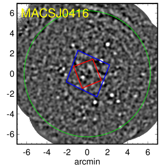
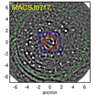
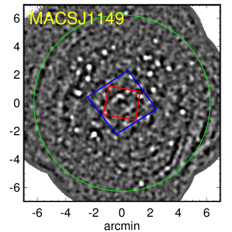
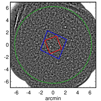
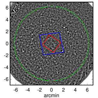
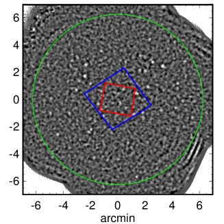
Figure 1.— 850 $\mu$m (top) and 450 $\mu$m (bottom) S/N maps of the three Frontier Fields, MACS J0416.1–2403, MACS J0717.5+3745 and MACS J1149.5+2223. The blue and red boxes represent, respectively, the positions of ACS and WFC3 coverage for the Frontier Field program. The green circles show the coverage of our VLA 6 GHz observations. Our 3 GHz images cover four times the area of the 6 GHz observations. In this work, we focus on the areas of HST coverage.

Table 1Summary of JCMT/SCUBA-2 observations

Field	R.A.	Decl.	Redshift	Weather	Exposure	${\sigma}$
					(hr)	(mJy beam-1)
MACS J0416.1–2403	04 16 08.9	$-$24 04 28.7	0.396	1+2+3	24.0+1.0+4.0	[2.31,0.36]
MACS J0717.5+3745	07 17 34.0	37 44 49.0	0.545	1+2+3	30.7+8.0+1.5	[2.03,0.34]
MACS J1149.5+2223	11 49 36.3	22 23 58.1	0.543	1+2+3	29.0+3.5+3.4	[1.63,0.30]

2.2. VLA Images

The VLA observations were carried out in the A (maximum baseline = 36.4 km) and the C (maximum baseline = 3.4 km) configurations using both the S-band (2-4 GHz) and C-band (4-8 GHz) receivers. For the S band, two 1 GHz Intermediate Frequency (IF) band pairs were used, both with right- and left-hand circular polarization, and sampled at 8 bits, while for the C band two 2 GHz IF band pairs were utilized with 3 bit sampling. The 1 and 2 GHz-wide bands were then divided by the WIDAR correlator into 8 and 16 128 MHz wide spectral windows, respectively, each with 64 spectral channels and four polarization products (RR, LL, RL, and LR). The on-source integration times for each of the three targets, in each of these band / configuration pairs are given in Table 2, along with the equatorial coordinates of the targets themselves. The primary and secondary calibrators are also listed for each target.

Table 2Summary of VLA observations, including calibrators and the on-source integration times for each configuration/band pairings.

		Band	Config	MACS J0416.1–2403	MACS J0717.5+3745	MACS J1149.5+2223
Primary cal				3C48	3C147	3C286
Secondary cal		S		J0416-1851	J0714+3534	J1158+2450
Secondary cal		C		J0416-1851	J0714+3534	J1150+2417
Integration time	(hr)	S	A	35.2	25.2	27.3
Integration time	(hr)	S	C	1.92	1.52	1.57
Integration time	(hr)	C	A	18.8	13.7	13.9
Integration time	(hr)	C	C	1.05	0.56	0.62

The data of each individual observing session were initially processed using the NRAO VLA pipeline. This is a set of scripts for the Common Astronomy Software Applications (CASA; McMullin et al., 2007) package designed to perform basic calibration steps on continuum data for total intensity (Stokes I) science. After Hanning-smoothing, the pipeline performs various data editing steps such as the flagging of data due to antenna shadowing, visibilities with amplitudes that are exactly zero, and integrations when the antennas are not one-source. A first pass of radio frequency interference (RFI) excision from the calibrator and target scans is performed using a sliding window statistical filter. The pipeline also performs delay and bandpass calibration using the primary calibrators. Time-dependent antenna-based complex gain corrections are derived using the secondary calibrator and interpolated for application to the target scans. A gain correction is derived independently for each spectral window.

Following the execution of the pipeline, the target field from each pointing was split into a single measurement set. The CASA mstransform task was then used to add a WEIGHT_SPECTRUM column to the visibilities. This column has the same shape as the DATA column and allows a unique weight to be assigned to each visibility point for use in subsequent imaging. The statwt task was then used to adjust values in the WEIGHT_SPECTRUM based on the time-dependent statistical properties of the visibilities for each baseline. This step (often) proves to be effective at suppressing low-level RFI or other issues with the data that are missed by the automated flagging routines.

The target fields were then imaged using the wsclean software (Offringa et al., 2014) and Briggs weighting (robustness parameter $=$ 0.2), producing images of 16,384 $\times$ 16,384 pixels, with pixel sizes of 0$\farcs$1 and 0$\farcs$06 for S and C bands, respectively. Images were produced for each band and each cluster by jointly gridding and deconvolving all of the relevant measurement sets. Spectral behavior of the sources (both intrinsic toward the beam center, and instrumentally perturbed off-axis) was captured during deconvolution by imaging the data in four spectral sub-bands across the band. The approach used by wsclean during deconvolution is to find peaks in the full-band image and then deconvolve these in each sub-band independently. For major-cycle purposes, clean components were fitted by a second order polynomial when predicting the visibility model. Cleaning was terminated after 100,000 iterations or when a the peak pixel in the full-band residual map reached a threshold of 1.0 $\mu$Jy, whichever occurred sooner. Imaging concludes with the model being restored into the full-band residual map, using a 2D Gaussian as fitted to the main lobe of the point spread function as the restoring beam. The data from both configurations (A and C) were combined during deconvolution and imaging. In Table 3, we provide the synthesized beams of the images for both bands. We caution that the small beams of these images might resolve out some extended emission and therefore miss some sources.

The primary beam sizes (HPBW) are $\sim$ 14^′ at S band and $\sim$ 7^′ at C band. Primary beam correction was applied to the final image by dividing it by a model of the VLA Stokes-I beam at the band center. The model itself was obtained by running the CASA clean task and using the predicted sensitivity (.flux) image. This is a somewhat crude approach for data with such a large fractional bandwidth; however (1) primary beam correction via projection-based gridding is not yet viable, and (2) the band center beam model differs from the zeroth-order Taylor-term beam model predicted by the widebandpbcor task by a couple of percent at most, so for our purposes the approaches are essentially equivalent.

The data reduction at this stage is designed to provide an initial set of Stokes-I images at S and C bands. Improvements in the imaging is possible via self-calibration techniques and this work is on-going. In-band and dual band (S–C) spectral index maps will be produced once the calibration is finalized. The observations were also scheduled to allow polarimetric calibration, and this is also forthcoming.

Table 3Synthesized beams of the 3 and 6 GHz images for each field.

		3 GHz			6 GHz
Field	$b_{\rm max}$	$b_{\rm min}$	$b_{\rm PA}$	$b_{\rm max}$	$b_{\rm min}$	$b_{\rm PA}$
MACS J0416.1–2403	0$\farcs$81	0$\farcs$42	0.65∘	0$\farcs$47	0$\farcs$24	20.96∘
MACS J0717.5+3745	0$\farcs$49	0$\farcs$44	78.29∘	0$\farcs$27	0$\farcs$23	-76.10∘
MACS J1149.5+2223	0$\farcs$44	0$\farcs$41	33.38∘	0$\farcs$24	0$\farcs$22	46.37∘

2.3. HST Images and Photometry

We retrieved the HST Frontier Fields images and the HST images from the Cluster Lensing And Supernova survey with Hubble (CLASH; Postman et al. 2012) archive for the passbands that are not included in the Frontier Fields program. We ran SExtractor (Bertin & Arnouts, 1996) in dual-image mode using F814W and F160W as detection bands to produce two sets of photometric catalogs. The deblending parameters deblend_nthresh and deblend_mincont were set to be 32 and 0.005, respectively. For a source that is within the WFC3 coverage, we use the F160W-detected photometry instead of the F814W-detected one.

2.4. Spitzer Images and Photometry

We retrieved the Spitzer Frontier Fields data at 3.6 and 4.5 $\mu$m, and we used the Spitzer image processing package mopex (Makovoz & Khan, 2005; Makovoz & Marleau, 2005; Makovoz et al., 2006) to extract sources. Photometry estimation and deblending were performed by the default Point Response Function (PRF) fitting algorithm.

2.5. Other Ancillary Data and Photometric Catalogs

Brammer et al. (2016) recently provided deep, calibrated $K_{s}$-band images of all six of the Hubble Frontier Fields using the instruments HAWK-I on the VLT and MOSFIRE on the Keck I telescope. We retrieved the images of our three cluster fields and ran SExtractor to perform source extraction. We also obtained the images and photometric catalogs from the CLASH archive that were obtained with Supreme-Cam on the Subaru telescope, WIRCam and MegaCam on the Canada–France–Hawaii telescope (CFHT), as well as the source catalogs of Herschel PACS and SPIRE passbands from the Herschel Lensing Survey (Rawle et al., 2016).

3. Sample Selection

3.1. SCUBA-2 Source Extraction

In this work, we focus on 850 $\mu$m selected sources, and we detected sources down to a 4$\,\sigma$ level. Casey et al. (2013) and Chen et al. (2013a, b) have shown that sources detected above a 4$\,\sigma$ level from their SCUBA-2 maps (with central 1$\,\sigma$ sensitivity of $\sim$ 0.8 mJy at 850 $\mu$m) have a contamination rate of $\leq$ 5%. Following Hsu et al. (2016), we estimate the contamination rate by constructing the source-free ”jackknife maps” at both wavelengths. A jackknife map is a pure noise image with sources removed; it is created by subtracting one-half of the data from the other, then scaling each pixel value by a factor of $\sqrt{t_{1}\times t_{2}}/(t_{1}+t_{2})$, with $t_{1}$ and $t_{2}$ representing the integration time of each pixel from the two halves of data. In each field, we searched for 4$\,\sigma$ sources within the area where the noise values are less than three times the central noise (an area of $\sim$ 130 arcmin²). The ratio of the total number of sources from the jackknife maps and from the science maps is 10/292, or 3.4%. If we only consider the regions that are covered by HST/ACS, the ratio is 1/44, or 2.3%.

To perform source extraction, we generated the PSFs by averaging all the primary calibrators. Following the methodology of source extraction in Chen et al. (2013a, b) and Hsu et al. (2016), we identified the pixel with the maximum S/N, subtracted this pixel and its surroundings using the PSF centered and scaled at the position and value of this pixel, and then searched for the next maximum S/N. We iterated this process until the detection threshold was hit. We only selected sources in the areas covered by the HST Frontier Fields since these sources are the most highly lensed ones with deep HST photometry. There are 44 850 $\mu$m sources within the HST coverage. We then measured the 450 $\mu$m flux density of each 850 $\mu$m source by searching for the maximum 450 $\mu$m peak flux within the 850 $\mu$m beam.

3.2. Flux Deboosting

The flux densities we measured from the SCUBA-2 maps are boosted by both Eddington bias (Eddington, 1913) and confusion noise (Condon, 1974). In addition, the flux errors we obtained are purely from statistical/instrumental noise, which does not include the above effects. We therefore need to run Monte Carlo simulations to correct the measured flux densities and their uncertainties. To perform such simulations, one normally uses a number counts model to populate sources onto the jackknife map, runs source extraction on this map, and then compares the input and measured flux densities. In a lensed field, however, it is tricky to run these simulations because assumptions of a lens model and a source plane redshift are required to project the simulated sources onto the image plane and to magnify their fluxes.

Here we used a simpler but rather time-consuming method that does not require lens modeling. We added three sources into our science map with random flux densities at random positions at a time and then performed source extraction, recording the input and measured flux densities of the sources we inserted. We only used the central area of each map that is covered by the HST. Only a small number of sources were inserted at a time in order to avoid over-crowdedness, such that the flux measurements for these sources are not influenced by each other. We repeated this procedure until we obtained 50000 pairs of input and measured flux densities. An inserted source is considered to be recovered if it is detected within the HWHM of the SCUBA-2 beam from the original input position.

In Figure 2, we show the boosting factor as a function of detection S/N at 450 and 850 $\mu$m for MACSJ0416. The boosting factor is measured as the ratio of the measured and input flux densities. The red line in each panel of Figure 2 represents the median boosting factor, and the two blue lines enclose the 1$\,\sigma$ spread. We deboosted the flux densities of our sources in each map using the median boosting factor and the corresponding 1$\,\sigma$ uncertainty.

3.3. Confusion Limit at 850 $\mu$m

To estimate the confusion limit of SCUBA-2 observations at 850 $\mu$m, we use the formalism of Condon (1974) and define the beam size as $\Omega_{\rm b}=\pi({\rm FWHM}/2.35)^{2}$, where FWHM is 14$\farcs$5. Following Hogg (2001), an image is considered confused when the source density exceeds one source per 30 beams. We adopt a broken power law for the differential number counts

$$\frac{dN}{dS}=\left\{\begin{matrix}N_{0}\left(\frac{S}{S_{0}}\right)^{-\alpha}~{}~{}{\rm if}~{}S\leq S_{0}\\ N_{0}\left(\frac{S}{S_{0}}\right)^{-\beta}~{}~{}{\rm if}~{}S>S_{0}\end{matrix}\right.$$ (1)

We can then calculate the cumulative counts, $N(>S)$, which represents the number density of sources that are brighter than $S$. Equating $N(>S)$ and $1/30\Omega_{\rm b}$ leads to the confusion limit of blank fields

$$S_{\rm c}=\left\{\frac{\alpha-1}{N_{0}S_{0}^{\alpha}}\left[\frac{1}{30\Omega_{\rm b}}+N_{0}S_{0}\left(\frac{1}{\alpha-1}-\frac{1}{\beta-1}\right)\right]\right\}^{\frac{1}{1-\alpha}}$$ (2)

Adopting the best-fit parameters of the broken power law in Hsu et al. (2016), we obtain $S_{\rm c}=1.64$ mJy.

In a lensed field, the cumulative number counts become $N_{\rm lens}(>S)=N(>S/\mu)/\mu$, where $\mu$ is the lensing magnification and $S$ is the observed flux density. Equating $N_{\rm lens}(>S)$ and $1/30\Omega_{\rm b}$, we obtain the observed confusion limit, $S_{\rm c}$ (on the image plane), as a function of $\mu$. The confusion limit on the source plane is $S_{\rm c}/\mu$. The observed confusion limit is higher than that of blank fields, but on the source plane it is lower. For example, $S_{\rm c}$ and $S_{\rm c}/\mu$ are $\sim$ 1.93 and 0.96, respectively, for $\mu=2$.

Since we have detected sources down to a deboosted flux density of $\sim$ 1.4 mJy, many of them should be close to or below the observed confusion limit (which depends on $\mu$ and therefore position). As a consequence, we caution that our source detection at $S_{\rm 850\mu m}\lesssim$ 2 mJy is not complete because there must be sources that we missed due to source confusion.

3.4. VLA Source Extraction

Given the higher detection rate at 3 GHz than at 6 GHz, we used the 3 GHz images to search for the counterparts to our 850 $\mu$m sources. To extract the flux densities and positions of the 3 GHz sources, we first identified all the pixels that are local maxima and have S/N $\geq$ 5. We took the values of these pixels as the peak fluxes (per beam) of the sources. We then used the CASA imfit task to fit 2D Gaussian functions to measure another set of flux densities. Note that some of the flux densities measured with this method have S/N $<$ 5, but we still keep these sources given their well detected peak fluxes.

Using the source positions at 3 GHz as prior, we searched for the 6 GHz counterparts with 5$\,\sigma$-detected peak fluxes. For the sources that are not detected at 6 GHz, we measured their 5$\,\sigma$ limits at the 3 GHz positions. We again used imfit to measure a second set of flux densities for the detected 6 GHz sources. In addition, we measured another set of flux densities with imfit from the 6 GHz images that were convolved to match the beams of our 3 GHz images, using the CASA imsmooth task. This set of measurements along with the 3 GHz flux densities will be used to compute the spectral indices of our radio sources (Section 4.2). We adopted this procedure to counter the beam/resolution difference between the two bands.

Further discussion about the source extraction as well as its completeness and contamination rate will be presented in the upcoming paper, Heywood et al. (2017, in preparation).

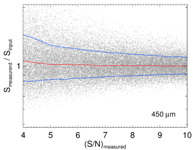
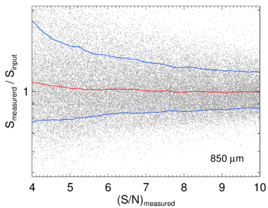
Figure 2.— Boosting factor as a function of detection S/N at 450 $\mu$m (left) and 850 $\mu$m (right) for MACS J0416.1–2403 from our Monte Carlo simulations. The boosting factor is measured as the ratio of the measured and input flux densities. The red line in each panel represents the median boosting factor, and the two blue lines enclose the 1$\,\sigma$ spread. We deboosted the flux densities of our sources in each map using the median boosting factor and the corresponding 1$\,\sigma$ uncertainty.

3.5. Counterpart Identification at 3 GHz

We used the corrected-Poissonian probability (Downes et al., 1986), the so-called $p$-values, as well as redshift cuts to perform counterpart identification. A radio source is considered the counterpart to the SCUBA-2 source if $p<0.05$ and its redshift is higher than the corresponding cluster redshift. The $p$-value is defined as $p=1-exp(\pi n\theta^{2})$, where $n$ is the radio source density and $\theta$ is the offset between the radio and the submillimeter sources. We adopted the redshift cuts as well because galaxies at redshifts lower than the cluster redshifts are not the lensed, faint galaxies that we are interested in. Besides, 850 $\mu$m selected SMGs have been mostly found at $z>0.5$ (Chapman et al., 2003, 2005). Therefore, those low-redshift galaxies are most likely just random radio sources that are not associated with our SCUBA-2 sources.

A total of 17 radio sources have $p<0.05$, four of which have spectroscopic redshifts (Ebeling et al. 2014; Schmidt et al. 2014; Grillo et al. 2015; Treu et al. 2015; Balestra et al. 2016). We used the BPZ code (Bayesian photometric redshift estimation; Benítez 2000) and the default galaxy templates (Benítez et al., 2004; Coe et al., 2006) to compute the photometric redshifts of those galaxies without spectroscopic redshifts. We fitted the templates to the HST photometry using isophotal magnitudes and obtained robust photometric redshifts for the sources that are detected in at least four bands (but not four ACS bands exclusively). One source in MACSJ0717 (0717-1 in Table 4) is only covered in three HST/ACS bands but is covered in the Subaru and CFHT images from CLASH. For this source, we simply took the photometric redshift ($z=1.14^{+0.07}_{-0.10}$) from the CLASH Subaru catalog. We corrected all of the magnitudes for Galactic dust extinction from Schlafly & Finkbeiner (2011) before running BPZ.

For the sources without spectroscopic and photometric redshifts (0416-4 and 0717-2 in Table 4), we used their 450 $\mu$m-to-850 $\mu$m flux ratios to crudely estimate the source redshifts. We converted the flux ratios to redshifts using a modified blackbody spectral energy distribution (SED) of the form $S_{\nu}\propto(1-e^{-\tau(\nu)})B_{\nu}(T)$, where $\tau(\nu)=(\nu/\nu_{0})^{\beta}$ and $\nu_{0}=3000$ GHz, assuming $\beta=1.5$ and dust temperature of 41.2 K. We chose this value of the dust temperature based on the results of our model fits to the FIR photometry, which we will describe in Section 4.1.

We removed two of these 17 radio sources with $p<0.05$ because of their low redshifts. Our final sample therefore consists of 14 SCUBA-2 sources and 15 3 GHz counterparts (one doublet). Only five of the SCUBA-2 sources (six of the radio counterparts) are detected at 6 GHz with peak fluxes above a 5$\,\sigma$ level. We show the 3 GHz and HST/ACS images of this final sample in Figure 3. Table 4 gives the coordinates, redshifts, observed SCUBA-2 and radio flux densities of these galaxies. It is possible that a radio counterpart is not responsible for the total emission of the corresponding 850 $\mu$m source, given that blended multiples are common for single-dish submillimeter sources (e.g., Wang et al. 2011; Barger et al. 2012; Smolčić et al. 2012; Hodge et al. 2013; Bussmann et al. 2015; Simpson et al. 2015). However, in this work, we assume that these 15 radio sources contribute the total 850 $\mu$m emission, in order to derive the IR properties of our 14 SCUBA-2 sources (Section 4.1). Submillimeter/millimeter interferometry is the only method to find out whether there are other radio-faint counterparts to these SCUBA-2 sources.

Cowie et al. (2017) inspected the positional uncertainty of the SCUBA-2 850 $\mu$m sources detected in the Chandra Deep Field-North (CDF-N). They found that the offsets between the SCUBA-2 positions and the SMA positions or the 1.4 GHz counterparts are all $<$ 4$\farcs$5 for 102 sources with 850 $\mu$m flux densities above 2 mJy. In our final sample, only 0717-4 has an offset of $\sim$ 5$\farcs$1 between the radio and submillimeter positions, and the others have offsets of $<$ 4$\farcs$5. Besides, $p=0.05$ essentially corresponds to matching radii of $\sim$ 5$\farcs$2, 5$\farcs$2, and 4$\farcs$3 for MACSJ0416, MACSJ0717, and MACSJ1149, respectively. Our results are therefore quite consistent with what Cowie et al. found. If we chose a fixed matching radius of 4$\farcs$5 and the same redshift cuts for counterpart matching, we would obtain a sample of 14 SCUBA-2 sources with only one source different from 0717-4.

3.6. Lens Models

In order to compute the intrinsic flux densities, luminosities, and SFRs of our lensed SMGs, the lensing magnifications are required, which depend on both the source redshifts and the lens models of the clusters. A set of lens models from eight independent teams are available for the HST Frontier Fields. These teams include Bradac (Bradač et al., 2005, 2009; Hoag et al., 2016), CATS (Jullo & Kneib, 2009; Jauzac et al., 2012, 2014, 2015a, 2015b; Richard et al., 2014), Diego (Diego et al., 2005a, b, 2007, 2015), GLAFIC (Oguri, 2010; Kawamata et al., 2016), Merten (Merten et al., 2009, 2011), Sharon (Jullo et al., 2007; Johnson et al., 2014), Williams (Liesenborgs et al., 2006; Mohammed et al., 2014; Grillo et al., 2015; Sebesta et al., 2016), and Zitrin (Zitrin et al., 2009, 2013).

Following Coe et al. (2015), we estimated the median and 68.3% range of the magnification values from the full range of each model in the HST Frontier Fields archive as well as the uncertainties of the source redshifts. The Merten models are excluded in our estimations because they have much lower resolution (8$\farcs$33). For each field, we used the newest model from each team. However, because different models have different spatial coverage, different sources in the same field are often not covered by the same amount of lens models.

In order to be consistent for the sources in the same field, for MACSJ0416 and MACSJ0717, we only used the models that cover all the sources in each field. However, for MACSJ1149, only the CATS and Sharon models can cover all the six sources, which would result in much smaller systematic errors of magnifications than those of the sources in the other two fields. Ideally, at least three models should be included to examine the systematic effect on the magnifications. We therefore used a set of four models, which all cover 1149-1, 1149-2, 1149-3, 1149-4, and 1149-6, and a different set of three models (all the available models) for 1149-5. In Table 5, we tabulate the models we included and the resulting lensing magnification for each of our sources.

Table 4Coordinates and redshifts, as well as SCUBA-2 and VLA flux densities of the 3 GHz identified sample of 850 $\mu$m sources

ID	R.A.	Decl.	Redshift	$S_{850\mu{\rm m}}$	$S_{450\mu{\rm m}}$	$S_{\rm 3GHz,peak}$	$S_{\rm{3GHz,fit}}$	$S_{\rm 6GHz,peak}$	$S_{\rm{6GHz,fit}}$	$S_{\rm{6GHz-cv,fit}}$
				(mJy)	(mJy)	($\mu$Jy beam-1)	($\mu$Jy)	($\mu$Jy beam-1)	($\mu$Jy)	($\mu$Jy)
0416–1	04 16 10.80	$-$24 04 47.6	2.087 (s)	4.38 $\pm$ 0.72	14.5 $\pm$ 3.5	8.0 $\pm$ 1.0	14.7 $\pm$ 3.3	$<4.3$	…	…
0416–2	04 16 13.23	$-$24 03 19.8	0.9063 (s)	2.22 $\pm$ 0.79	7.5 $\pm$ 3.5	12.2 $\pm$ 1.1	27.8 $\pm$ 4.1	$<5.6$	…	…
0416–3	…	…	…	2.18 $\pm$ 0.79	14.1 $\pm$ 4.0	…	…	…	…	…
0416–3–1	04 16 09.68	$-$24 05 55.4	0.99 $\pm$ 0.10 (p)	…	…	31.1 $\pm$ 1.1	55.4 $\pm$ 3.7	10.4 $\pm$ 1.1	20.8 $\pm$ 3.5	32.9 $\pm$ 4.6
0416–3–2	04 16 09.64	$-$24 05 55.2	1.01 $\pm$ 0.10 (p)	…	…	29.5 $\pm$ 1.1	31.9 $\pm$ 2.4	13.0 $\pm$ 1.1	17.0 $\pm$ 2.4	18.5 $\pm$ 2.6
0416–4	04 16 12.96	$-$24 05 43.0	2.7${}^{+2.7}_{-2.2}$ (r)	1.78 $\pm$ 0.83	5.5 $\pm$ 3.4	11.8 $\pm$ 1.0	13.6 $\pm$ 2.1	5.7 $\pm$ 1.0	9.0 $\pm$ 2.3	8.6 $\pm$ 2.3
0717–1	07 17 24.55	37 43 29.7	1.14${}^{+0.07}_{-0.10}$ (p)	5.65 $\pm$ 0.88	18.7 $\pm$ 3.9	6.8 $\pm$ 0.9	18.2 $\pm$ 3.4	$<6.2$	…	…
0717–2	07 17 38.15	37 46 17.0	4.5${}^{+2.3}_{-1.3}$ (r)	3.25 $\pm$ 0.68	4.9 $\pm$ 2.9	5.6 $\pm$ 1.0	5.1 $\pm$ 1.5	$<5.5$	…	…
0717–3	07 17 33.20	37 44 01.5	1.54 $\pm$ 0.13 (p)	2.21 $\pm$ 0.61	7.2 $\pm$ 2.9	6.5 $\pm$ 1.1	15.2 $\pm$ 3.5	$<5.3$	…	…
0717–4	07 17 32.40	37 43 19.7	0.78 $\pm$ 0.09 (p)	2.24 $\pm$ 0.69	6.9 $\pm$ 3.1	42.1 $\pm$ 1.0	48.9 $\pm$ 1.9	18.2 $\pm$ 1.0	24.3 $\pm$ 2.3	23.4 $\pm$ 1.6
1149–1	11 49 30.66	22 24 27.8	1.36 $\pm$ 0.12 (p)	4.75 $\pm$ 0.76	15.4 $\pm$ 2.7	5.2 $\pm$ 1.0	27.4 $\pm$ 8.3	$<4.9$	…	…
1149–2	11 49 36.07	22 24 24.5	1.28 $\pm$ 0.11 (p)	2.20 $\pm$ 0.61	5.7 $\pm$ 2.3	6.6 $\pm$ 1.0	14.1 $\pm$ 4.0	$<5.1$	…	…
1149–3	11 49 34.41	22 24 45.3	0.9754 (s)	2.23 $\pm$ 0.64	7.9 $\pm$ 2.6	14.4 $\pm$ 1.0	18.0 $\pm$ 2.0	8.0 $\pm$ 1.0	12.0 $\pm$ 2.3	12.4 $\pm$ 1.8
1149–4	11 49 35.47	22 22 32.0	1.24 $\pm$ 0.11 (p)	2.37 $\pm$ 0.69	4.1 $\pm$ 2.3	6.9 $\pm$ 1.0	12.5 $\pm$ 3.6	$<5.1$	…	…
1149–5	11 49 42.37	22 23 39.6	1.56 $\pm$ 0.13 (p)	1.93 $\pm$ 0.74	8.1 $\pm$ 2.9	10.0 $\pm$ 1.0	12.1 $\pm$ 2.1	5.3 $\pm$ 1.0	9.1 $\pm$ 2.6	7.3 $\pm$ 1.5
1149–6	11 49 40.14	22 22 33.4	0.93 $\pm$ 0.10 (p)	1.55 $\pm$ 0.77	3.1 $\pm$ 2.1	10.5 $\pm$ 1.0	17.2 $\pm$ 2.7	$<4.7$	…	…

Table 5lens models used for each source and the resulting magnification value.

ID	Magnification	Models
0416–1	1.83${}^{+0.54}_{-0.07}$	Bradac-v3  CATS-v3.1  Sharon-v3
0416–2	1.67${}^{+0.11}_{-0.14}$	”
0416–3	1.57${}^{+0.26}_{-0.42}$	”
0416–4	1.21${}^{+0.53}_{-0.08}$	”
0717–1	1.28 $\pm$ 0.16	Bradac-v1  CATS-v1  GLAFIC-v3  Sharon-v2  Zitrin-LTM-v1  Zitrin-LTM-Gauss-v1
0717–2	2.12${}^{+0.42}_{-0.36}$	”
0717–3	3.04${}^{+0.95}_{-0.43}$	”
0717–4	1.20${}^{+0.09}_{-0.07}$	”
1149–1	1.64${}^{+0.21}_{-0.35}$	CATS-v1  Sharon-v2.1  Zitrin-LTM-v1  Zitrin-LTM-Gauss-v1
1149–2	2.89${}^{+0.66}_{-0.54}$	”
1149–3	3.08${}^{+1.20}_{-0.44}$	”
1149–4	1.19${}^{+0.20}_{-0.08}$	”
1149–5	1.44${}^{+0.07}_{-0.18}$	CATS-v1  Sharon-v2.1  GLAFIC-v3
1149–6	1.18${}^{+0.10}_{-0.15}$	CATS-v1  Sharon-v2.1  Zitrin-LTM-v1  Zitrin-LTM-Gauss-v1

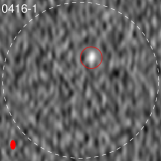
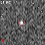
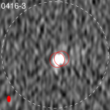
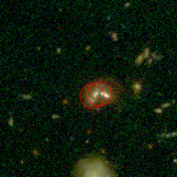
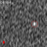
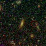
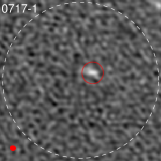
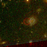
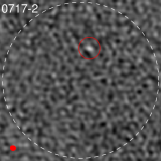
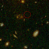
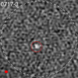
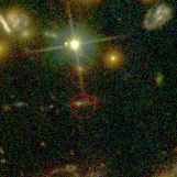
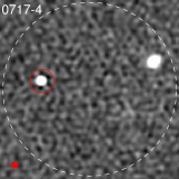
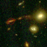
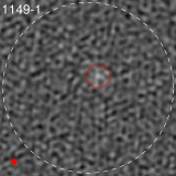
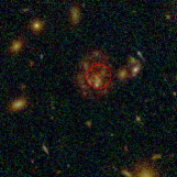
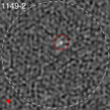
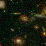
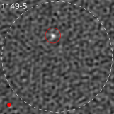
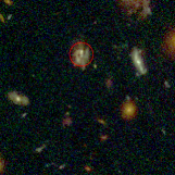
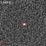
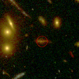
Figure 3.— 3 GHz identified sample of SCUBA-2 850 $\mu$m sources that are within the HST Frontier Fields coverage. For each source, we show the 3 GHz image on the left and the ACS false-color (F435W, F606W and F814W) image on the right. The image size is 15${}^{\prime\prime}\times$ 15^′′. In the 3 GHz images, the large dashed circles with a diameter of 14$\farcs$5 represent the JCMT beam (FWHM) at 850 $\mu$m. The positions of the 3 GHz counterparts are indicated by the 1^′′-radius red circles in both the 3 GHz and ACS images. The ellipse at the bottom-left corner of each 3 GHz image represents the synthesized beam. Note that another bright radio source also locates within the SCUBA-2 beam of 0717-4. However, this source is not considered the counterpart because $p>0.05$ and it is at $z\sim 0.3$.

Table 6Herschel and ALMA 1.1 mm flux densities from Rawle et al. (2016) and González-López et al. (2017).

ID	$S_{100\mu{\rm m}}$	$S_{160\mu{\rm m}}$	$S_{250\mu{\rm m}}$	$S_{350\mu{\rm m}}$	$S_{500\mu{\rm m}}$	$S_{1100\mu{\rm m}}$
	(mJy)	(mJy)	(mJy)	(mJy)	(mJy)	(mJy)
0416–1	5.1 $\pm$ 1.0	12.6 $\pm$ 2.0	(9.7 $\pm$ 3.1)	(6.8 $\pm$ 2.6)	…	1.32 $\pm$ 0.10
0416–2	11.1 $\pm$ 1.2	24.5 $\pm$ 2.2	(9.1 $\pm$ 3.5)	(4.7 $\pm$ 2.9)	…	…
0416–3	20.1 $\pm$ 1.7	36.4 $\pm$ 3.2	31.5 $\pm$ 3.9	24.2 $\pm$ 3.5	10.5 $\pm$ 3.7	…
0416–4	…	…	…	…	…	…
0717–1	3.8 $\pm$ 0.8	15.2 $\pm$ 1.8	31.0 $\pm$ 3.8	34.2 $\pm$ 4.7	16.9 $\pm$ 3.0	…
0717–2	…	…	…	…	…	…
0717–3	…	…	…	…	…	…
0717–4	…	…	…	…	…	…
1149–1	7.0 $\pm$ 0.9	16.4 $\pm$ 1.8	32.3 $\pm$ 3.2	30.3 $\pm$ 3.2	21.4 $\pm$ 2.8	…
1149–2	3.7 $\pm$ 0.7	7.9 $\pm$ 1.5	(5.9 $\pm$ 2.5)	…	…	0.58 $\pm$ 0.13
1149–3	7.7 $\pm$ 1.0	18.4 $\pm$ 1.9	23.7 $\pm$ 3.7	14.2 $\pm$ 3.0	6.1 $\pm$ 3.9	$<$ 0.57
1149–4	3.2 $\pm$ 0.7	9.6 $\pm$ 1.4	…	…	…	…
1149–5	5.0 $\pm$ 0.8	10.0 $\pm$ 1.4	12.5 $\pm$ 2.5	5.7 $\pm$ 2.8	…	…
1149–6	6.2 $\pm$ 0.9	11.3 $\pm$ 1.7	12.6 $\pm$ 2.6	7.4 $\pm$ 3.3	3.8 $\pm$ 3.4	…

Table 7Dust temperatures, IR luminosities, and SFRs

ID	$T$	$L_{\rm IR}$	SFRIR	SFR6GHz	SFRUV
	(K)	($10^{11}L_{\odot}$)	($M_{\odot}$ yr-1)	($M_{\odot}$ yr-1)	($M_{\odot}$ yr-1)
0416–1	51.2 $\pm$ 2.0	17.0${}^{+2.3}_{-3.4}$	253${}^{+34}_{-51}$	226${}^{+40}_{-71}$	28.2${}^{+1.2}_{-6.4}$
0416–2	41.2${}^{+2.4}_{-2.3}$	4.85${}^{+0.57}_{-0.49}$	72${}^{+8}_{-7}$	67 $\pm$ 11	2.3${}^{+0.2}_{-0.1}$
0416–3	44.8${}^{+2.6}_{-2.4}$	9.76${}^{+3.84}_{-2.31}$	146${}^{+57}_{-34}$	281${}^{+87}_{-45}$	5.6${}^{+2.0}_{-1.0}$
0416–4	…	…	…	519${}^{+1601}_{-482}$	…
0717–1	29.3 $\pm$ 1.8	8.34${}^{+1.52}_{-1.99}$	124${}^{+23}_{-30}$	99${}^{+23}_{-31}$	4.3${}^{+0.8}_{-1.2}$
0717–2	…	…	…	372${}^{+481}_{-225}$	…
0717–3	27.9${}^{+19.1}_{-8.9}$	…	…	70${}^{+20}_{-24}$	0.8 $\pm$ 0.2
0717–4	17.9${}^{+14.9}_{-5.8}$	…	…	112${}^{+27}_{-24}$	0.1${}^{+0.2}_{-0.1}$
1149–1	35.6${}^{+2.6}_{-2.5}$	10.9${}^{+2.4}_{-2.3}$	162${}^{+36}_{-34}$	176${}^{+75}_{-60}$	1.5${}^{+0.7}_{-0.4}$
1149–2	40.4${}^{+4.8}_{-3.8}$	2.40${}^{+0.61}_{-0.47}$	36${}^{+9}_{-7}$	44${}^{+14}_{-15}$	2.3${}^{+0.5}_{-0.4}$
1149–3	38.2${}^{+1.9}_{-1.7}$	2.43${}^{+0.51}_{-0.71}$	36${}^{+8}_{-11}$	28${}^{+7}_{-8}$	1.2${}^{+0.2}_{-0.3}$
1149–4	41.3${}^{+5.5}_{-4.8}$	5.47${}^{+1.25}_{-1.37}$	82${}^{+19}_{-20}$	89${}^{+29}_{-31}$	0.7 $\pm$ 0.1
1149–5	54.9${}^{+6.0}_{-5.2}$	8.50${}^{+1.56}_{-1.65}$	127${}^{+23}_{-25}$	121${}^{+40}_{-28}$	3.2${}^{+1.2}_{-0.8}$
1149–6	42.4${}^{+4.2}_{-4.0}$	3.65${}^{+1.01}_{-0.72}$	55${}^{+15}_{-11}$	63${}^{+21}_{-16}$	0.1 $\pm$ 0.1

4. Properties of Radio-detected Submillimeter Sources

4.1. Dust Temperatures and IR SFRs

We cross-match our final sample of SCUBA-2 sources with the source catalog from the Herschel Lensing Survey (Rawle et al., 2016). Using the 3 GHz positions as prior, 10 of the 14 sources have a nearest Herschel detection with an offset of $<$ 1^′′. On the other hand, the remaining four sources have no Herschel counterpart even when a 10^′′ matching radius is used. For the 10 sources with Herschel detections, the optical counterparts we identified completely agree with the optical counterparts Rawle et al. found. Additionally, 0416-1 and 1149-2 are detected by the Atacama Large Millimeter/submillimeter Array (ALMA) 1.1 mm imaging of González-López et al. (2017) as MACSJ0416-ID01 and MACSJ1149-ID01, respectively. We also estimate the 5$\,\sigma$ limit of 1.1 mm flux density for 1149-3, which is the only other source covered by the ALMA maps. The observed Herschel and ALMA 1.1 mm flux densities are shown in Table 6.

For four sources, we found that the Herschel/SPIRE photometry does not agree well with our SCUBA-2 flux densities. Compared with the SCUBA-2 photometry, the SPIRE SEDs of these sources turn over at shorter wavelengths. This inconsistency might be caused by the PSF-fitting procedure and/or deblending photometry performed by Rawle et al. (2016). We therefore decided to flag the SPIRE flux densities that are a factor of two lower than the best-fit modified blackbody models for the SEDs constructed from the Herschel/PACS, SCUBA-2, and ALMA (if available) photometry. These flags are done for 0416-1, 0416-2, and 1149-2, which are presented in Table 6 and Figure 4.

For the sources with spectroscopic or photometric redshifts, we measure their dust temperatures by fitting a modified blackbody model with $\beta=1.5$ (e.g., Chapman et al. 2005; Kovács et al. 2006; Pope et al. 2006) to the FIR flux densities. The resulting median dust temperature is 41.2${}^{+1.8}_{-2.0}$ K. We therefore use $\beta=1.5$ and $T=41.2$ K to estimate the redshifts for the remaining two sources (0416-4 and 0717-2) that have no redshift measurements. Note that only 450 and 850 $\mu$m flux densities are available for these two sources as well as 0717-3 and 0717-4 because they are not detected in Herschel Lensing Survey. As a consequence, what we do is simply match the models and the 450 $\mu$m-to-850 $\mu$m flux ratios instead of least chi-squared fitting.

We fit the templates of Rieke et al. (2009) to the FIR flux densities for the 10 sources that are detected by Herschel to derive their IR luminosities ($L_{\rm IR}$; $\lambda_{\rm rest}$ = 8-1000 $\mu$m). $L_{\rm IR}$ is then converted to SFR via the theoretical relation in Murphy et al. (2011). Both the $L_{\rm IR}$ and SFRs are corrected for the lensing magnifications based on our redshifts and the lens models. We do not compute the IR SFRs of 0416-4, 0717-2, 0717-3, and 0717-4 since they are only detected at 450 and 850 $\mu$m. We show these fits in Figure 4. All the derived quantities are listed in Figure 4 (without uncertainties) and Table 7.

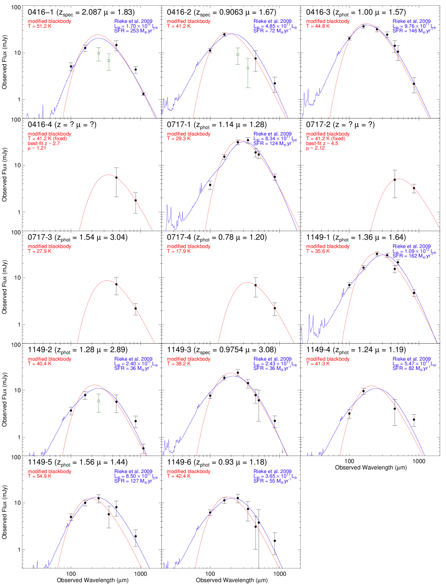
Figure 4.— FIR SEDs of our 3 GHz identified sample of SCUBA-2 850 $\mu$m sources that illustrate the observed photometry and fits. The flux densities are from Herschel/PACS (100 and 160 $\mu$m), Herschel/SPIRE (250, 350, and 500 $\mu$m), SCUBA-2 (450 and 850 $\mu$m), and ALMA (1.1mm). The Herschel and ALMA flux densities are from Rawle et al. (2016) and González-López et al. (2017), respectively. The SPIRE flux densities shown as green squares are flagged in the fits. In each panel, we plot the best-fit modified blackbody (red line) and Rieke et al. (2009) template (blue line). Derived quantities from the two models are shown in matching colors, including IR luminosities and SFRs, which take the magnifications ($\mu$) into account. 12 of the 14 sources have spectroscopic ($z_{\rm spec}$) or photometric ($z_{\rm phot}$) redshifts. For the two sources without redshifts, we use a modified blackbody with the median dust temperature from the other 11 sources (41.2 K) to convert their 450 $\mu$m-to-850 $\mu$m flux ratios to redshifts and therefore magnifications. The uncertainties of all the quantities are listed in Table 7.

4.2. Radio SFRs

Following Murphy et al. (2011, 2012), we compute the radio SFRs of our sources using the relation

$$\begin{split}\left(\frac{\rm SFR_{\nu}}{M_{\sun}\,{\rm yr^{-1}}}\right)&=10^{-27}\left[2.18\left(\frac{T_{\rm e}}{10^{4}\,{\rm K}}\right)^{0.45}\left(\frac{\nu}{\rm GHz}\right)^{-0.1}\right.+\\ &\left.15.1\left(\frac{\nu}{\rm GHz}\right)^{-\alpha^{\rm NT}}\right]^{-1}\left(\frac{L_{\nu}}{\rm erg~{}s^{-1}~{}Hz^{-1}}\right)\end{split}$$ (3)

where we assume an electron temperature of $T_{\rm e}=10^{4}$ K, and a constant non-thermal radio spectral index of $\alpha^{\rm NT}=0.85$, which is the average non-thermal spectral index found among the 10 star-forming regions in NGC 6946 studied by Murphy et al. (2011). Since our sources are all detected at 3 GHz and have a median redshift close to one, we decide to compute the rest-frame 6 GHz SFRs. In order to $K$-correct an observed radio flux density to rest-frame 6 GHz, we need the radio spectral index, $\alpha$, which relates the radio flux density with frequency via a power law $S_{\nu}\propto\nu^{-\alpha}$. We can then calculate the rest-frame 6 GHz radio luminosities using

$$L_{\nu_{\rm rest}}({\rm 6~{}GHz})=4\pi d_{L}^{2}S_{\nu_{\rm obs}}({\rm 3~{}GHz})(1+z)^{\alpha-1}\times 2^{-\alpha}$$ (4)

where $d_{L}$ is the luminosity distance. This calculation includes a bandwidth compression term of $(1+z)^{-1}$ and a color term of $(\frac{2}{1+z})^{-\alpha}$. For the six radio sources that are detected at both bands, we directly compute their spectral indices using the flux densities measured from the 3 GHz images and the convolved 6 GHz images with the Gaussian fitting procedure. We obtain an average of 0.76 $\pm$ 0.12 from these six sources, which is consistent with the values in the literature (e.g., Ibar et al. 2009; Ivison et al. 2010a, b). We assume this value for the other sources. The resulting radio SFRs are tabulated in Table 7.

4.3. UV SFRs

While the radio and IR SFRs represent the total and dust-obscured SFRs, respectively, the unobscured contributions from the (observed) UV emission should be accounted as well, given that most of our sources are detected in the optical images. We use rest-frame 2271 $\rm\AA$ (GALEX NUV band) flux densities and the conversion in Murphy et al. (2012) to compute the UV SFRs of our sources without extinction correction. We interpolate the HST photometry to obtain rest-frame 2271 $\rm\AA$ flux densities and then compute $L_{\rm NUV}$ and UV SFRs. These UV SFRs are also tabulated in Table 7, along with radio and IR SFRs. In Figure 5, we compare the radio SFRs with the IR+UV SFRs for the 10 sources that have IR SFR measurements. The UV SFRs are mostly too small to significantly affect the comparison except for 0416-1.

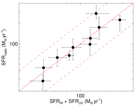
Figure 5.— Comparison between the radio SFRs and the IR+UV SFRs for the 10 sources that have IR SFR measurements. These SFRs are corrected for the lensing magnifications. The red solid line is the one-to-one relation. All of the 10 sources are within a multiplicative factor of two about the one-to-one line (the two red dashed lines).

4.4. 850 $\mu$m Flux Density to SFR Conversion

The observed (but de-lensed) 850 $\mu$m flux density of an SMG should work as a proxy of the IR luminosity and IR SFR independent of redshift since the strong negative $K$-correction and the effect of distance almost exactly cancel out (e.g., Blain & Longair 1993; Blain et al. 2002). Barger et al. (2014) and Cowie et al. (2017) have both measured the mean conversion between observed 850 $\mu$m flux density and IR SFR from their samples, with a multiplicative range over the individual values of two in each direction about the mean. Here we perform the same exercise, comparing our observed 850 $\mu$m flux densities and IR SFRs for the 10 sources that have IR SFR measurements in Figure 6. The median conversion of these sources is ${\rm SFR}_{\rm IR}(M_{\odot}~{}\rm{yr}^{-1})$ $=54\times S_{850\mu{\rm m}}$ (mJy), which is more than a factor of two smaller than the conversion (143) found in Cowie et al. (2017). However, the median redshifts of the two samples are $z=1.24$ (this work) and $z=2.28$ (Cowie et al.). Therefore, it is not surprising to see different properties between the two samples.

The large difference of $\left\langle{\rm SFR}_{\rm{IR}}/S_{850\mu{\rm m}}\right\rangle$ between the two studies is caused by the different SEDs of the two samples. If we only consider the cold dust emission at FIR wavelengths, the mean SED of our sample is close to a modified blackbody with $\beta=1.5$ and $T=41.2$ K. The sources in Cowie et al. (2017), on the other hand, are generally well described by an optically thin modified blackbody ($S_{\nu}\propto\nu^{\beta}B_{\nu}(T)$) with $\beta=1.25$ and $T=43$ K. If the modified blackbody model in this work is used, the resulting dust temperature would be $\sim$ 50 K. The main difference between these two samples is therefore in the dust temperature (or equivalently, the peak wavelength $\lambda_{\rm peak}$), and they make more than a factor of two difference in the contribution to IR luminosity at the same redshift.

The variation of ${\rm SFR}_{\rm{IR}}/S_{850\mu{\rm m}}$ among our sources is also a result of different dust temperatures. The three higher outliers in Figure 6 are 0416-1, 0416-3, and 1149-5, which have higher dust temperatures than the rest of the sample. In contrast, the only lower outlier in Figure 6 is 0717-1, which has the lowest dust temperature among the 10 sources that have IR SFR measurements. Note that different contributions from the emission at shorter wavelengths can be another cause of the different ${\rm SFR}_{\rm{IR}}/S_{850\mu{\rm m}}$. This result shows that our sample of low-redshift faint SMGs has lower dust temperatures (longer $\lambda_{\rm peak}$) than those of the bright SMGs, in agreement with other studies (e.g., Casey et al. 2012; U et al. 2012; Lee et al. 2013; Symeonidis et al. 2013).

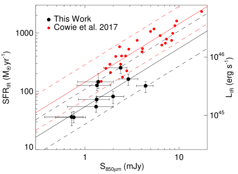
Figure 6.— Comparison between the 850 $\mu$m flux densities and IR SFRs/luminosities for the 10 sources that have IR SFR measurements. Both of these quantities are corrected for the lensing magnifications. The black solid line is the median conversion of these 10 sources, ${\rm SFR_{IR}}(M_{\odot}~{}\rm{yr}^{-1})$ $=54\times S_{850\mu{\rm m}}$ (mJy), and the black dashed lines correspond to a multiplicative factor of two about the black solid line. The red circles are the spectroscopic sample of SMGs from Cowie et al. (2017), and the red solid line is their mean conversion, ${\rm SFR_{IR}}(M_{\odot}~{}\rm{yr}^{-1})$$=143\times S_{850\mu{\rm m}}$ (mJy). The red dashed lines correspond to a multiplicative factor of two about the solid red line. The median redshifts of the two samples are $z=1.24$ (this work) and $z=2.28$ (Cowie et al.). The large difference of conversion factors between the two studies is caused by the different SEDs of the two samples.

4.5. Individual Sources

Here we describe some details for several galaxies that have special properties.

4.5.1 0416-1 and 0416-3

0416-1 is classified as an AGN in the Grism Lens-Amplified Survey from Space (GLASS; Schmidt et al. 2014; Treu et al. 2015). Because it is unclear whether the radio and UV emission is dominated by the AGN or star formation, we caution that the radio and UV SFRs for this source can only be considered as upper limits. The optical morphology of 0416-1 shows two peaks with a $\sim$ 0$\farcs$4 offset, suggesting that it might be a merger. 0416-3 has a pair of radio counterparts that are slightly blended at 3 GHz but clearly separated at 6 GHz. These two radio sources correspond to two galaxies that have photometric redshifts of $0.99\pm 0.10$ and $1.01\pm 0.10$. Both of the radio centers have $\sim$ 0$\farcs$5 offsets from the optical centers. These offsets and the consistent photometric redshifts suggest that the two galaxies are an interacting pair.

4.5.2 0416-4 and 0717-2

0416-4 and 0717-2 are the two sources without photometric redshifts. We show the $K_{s}$-band images of these two SMGs in Figure 7. Both of these sources are outside the WFC3 coverage and not detected by Herschel. The HST magnitudes of 0416-4 are only well measured in F425W, F606W, F814W, and F850LP; a photometric redshift of $z=$ 1.24${}^{+1.99}_{-0.46}$ is reported in the CLASH catalog. The large difference between the observed brightness at optical wavelengths and $K_{s}$ band for this source suggests it is likely at high redshift. We obtained a redshift estimate of $z=$ 2.7${}^{+2.7}_{-2.2}$ based on the 450 $\mu$m-to-850 $\mu$m flux ratio. 0717-2 is completely undetected in the HST images and also very faint in the Keck/MOSFIRE $K_{s}$-band image. This source would be an example of faint SMGs that are not included in the UV star formation history. Our redshift estimate for this source based on the 450 $\mu$m-to-850 $\mu$m flux ratio is $z=$ 4.5${}^{+2.3}_{-1.3}$.

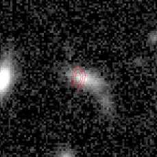
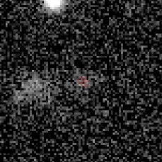
Figure 7.— $K_{s}$-band images (Brammer et al., 2016) of 0416-4 (left) and 0717-2 (right) centered at the 3 GHz positions. The red contours are (3.0, 6.0, 9.0)$\times\sigma$ (left) and (3.0, 5.0)$\times\sigma$ (right) isophotes of the 3 GHz sources, where $\sigma\sim$ 1.0 $\mu$Jy beam^-1 for both sources. The image size is 8${}^{\prime\prime}\times$ 8^′′

4.5.3 0717-1

The radio position of 0717-1 is $\sim$ 1$\farcs$5 east from the center of a spiral galaxy at $z=1.14$. A close-up HST/ACS image for this source in shown in Figure 8. This source is not within the WFC3 coverage. We can see faint and red structures at the radio position. It is not clear whether these structures are from a background lensed galaxy or are related to the spiral galaxy. We assumed the case of being related to the spiral galaxy to derive the properties of this SMG. In this case, the red structures might be the core and tidal tails of a smaller disrupted galaxy that is being merged into the larger spiral galaxy. Note that if this SMG is actually a background source at a higher redshift, the derived SFRs and dust temperature would all be higher.

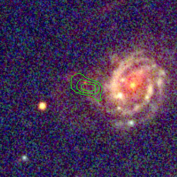
Figure 8.— Close-up HST/ACS false-color (F435W, F606W and F814W) image of 0717-1 centered at the 3 GHz position. The green contours are (3.0, 4.5, 6.0)$\times\sigma$ isophotes of the 3 GHz source, where $\sigma\sim$ 0.93 $\mu$Jy beam^-1. The image size is 6${}^{\prime\prime}\times$ 6^′′

Figure 9.— Counterpart identification rate as a function of observed (not de-lensed) 850 $\mu$m flux density for the 44 SCUBA-2 sources within the HST coverage. The flux range is $\sim 1.4-5.7$ mJy. Each bin includes 11 sources and is plotted at the mean flux density. The errors are based on Poisson statistics.

5. Detectability of the Submillimeter sources

5.1. Bias and Redshift Distribution

In the three Frontier Fields, there are 44 SCUBA-2 850 $\mu$m sources within the HST coverage, and we only found 15 radio counterparts to 14 of them. 13 of these 14 identified sources are detected in the optical images. All of the sources are detected in $K_{s}$ band, 3.6 $\mu$m, and 4.5 $\mu$m. 11 are at $z<2$, and the median redshift of the entire sample is $z=1.28^{+0.07}_{-0.09}$ (0416-3 is counted as one source at $z=1.00$). This is much lower than the redshift distribution of the classical SMGs, which are typically found to be at $z=2-3$ (e.g., Wardlow et al. 2011; Smolčić et al. 2012; Casey et al. 2013; Weiß et al. 2013; Simpson et al. 2014; Koprowski et al. 2016). The redshift distribution of our sample, which is lower than the classical SMGs, and the fact that we still miss about two-thirds of the SMGs in our radio images are caused by the bias of the radio identification technique. However, we note that some studies have suggested a “cosmic downsizing” (Cowie et al., 1996) of SMG luminosities (e.g., Heavens et al. 2004; Bundy et al. 2006; Franceschini et al. 2006; Dye et al. 2008; Mobasher et al. 2009; Magliocchetti et al. 2011; Hsu et al. 2016; Cowie et al. 2017). Therefore, fainter SMGs might indeed have a lower redshift distribution.

We show the counterpart identification rate as a function of observed 850 $\mu$m flux density in Figure 9. As expected, the identification rate is lower at fainter flux bins. Also, at the brightest flux bin ($\sim$ 3.4 mJy), 55% of the sources are still not identified. Those sources without radio counterparts are likely at higher redshifts. To estimate the depth of our 3 GHz survey in terms of detecting faint SMGs, we consider a source with a specific observed 850 $\mu$m flux density. Assuming that the UV SFR is negligible and $\rm{SFR_{radio}\sim SFR_{IR}}$, we can use equation (1) and our median $S_{850\mu{\rm m}}$–SFR_IR conversion in Section 4.4 to obtain the radio power $L_{\nu}$ at any rest-frame frequency. We can then compute the observed-frame 3 GHz flux density of this source as a function of redshift, as shown in Figure 10. This shows that, with our 5$\,\sigma$ detection limit of $\sim$ 5 $\mu$Jy beam^-1 at 3 GHz, we can only detect sources with observed $S_{850\mu{\rm m}}=$ 2 mJy out to $z\sim 1.9$. A higher ${\rm SFR}_{\rm{IR}}/S_{850\mu{\rm m}}$ would lead to a higher redshift limit, which should be the case for the three sources at $z>2$, 0416-1, 0416-4, and 0717-2. The value of ${\rm SFR}_{\rm{IR}}/S_{850\mu{\rm m}}$ for 0416-1 is 106. For 0416-4 and 0717-2, ${\rm SFR}_{\rm{IR}}/S_{850\mu{\rm m}}$ would be $>$ 200 if their IR SFRs agree with their radio SFRs.

We can also estimate a lower limit of the median redshift of all the 44 SCUBA-2 sources. Assuming all of the other 30 radio-faint SMGs are not blended multiples and they all have ${\rm SFR}_{\rm{IR}}/S_{850\mu{\rm m}}=54$, we can compute the lower redshift limit for each of these sources to be detected by our 3 GHz images. Along with the 14 SMGs we already identified, the median redshift of the entire sample is at $z>1.9$. In reality, some of these 30 sources would split into multiples, making the median redshift lower. Since a lower limit rather than an upper limit of the median redshift is estimated, it is not clear whether the redshift distribution of these cluster-lensed faint SMGs is indeed lower than those of the brighter samples. In addition, our estimated median redshift depends on the value of ${\rm SFR}_{\rm{IR}}/S_{850\mu{\rm m}}$. Because ${\rm SFR}_{\rm{IR}}/S_{850\mu{\rm m}}$ correlates with dust temperature (peak wavelength), the detectability of a SMG at 3 GHz is determined by both the dust temperature and the redshift. Therefore, future submillimeter interferometry is required to identify the multi-wavelength counterparts to the SCUBA-2 sources without radio counterparts, breaking the degeneracy of redshift and dust temperature distributions.

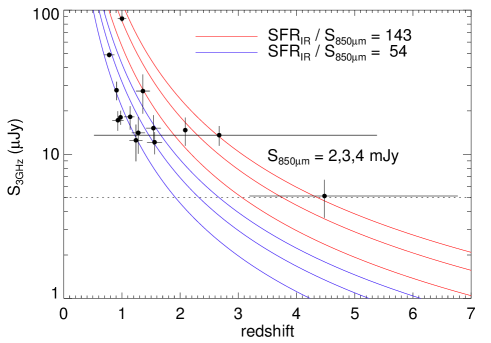
Figure 10.— Expected observed (not de-lensed) 3 GHz flux density as a function of redshift with different observed (not de-lensed) 850 $\mu$m flux densities based on the $S_{850\mu{\rm m}}$–SFR_IR conversions of this work (blue) and Cowie et al. (red; 2017). For each conversion, we plot the expected relations for $S_{850\mu{\rm m}}=$ 2, 3, and 4 mJy (bottom to top). The horizontal dashed line corresponds to our detection limit of $\sim$ 5 $\mu$Jy. Our sample of 14 SMGs are overplotted as black circles. We can only detect sources with observed $S_{850\mu{\rm m}}=$ 2 mJy out to $z\sim 1.9$ if ${\rm SFR}_{\rm{IR}}/S_{850\mu{\rm m}}=54$.

Figure 11.— $K$ – [4.5] color (Wang et al., 2012) versus redshift for the 14 radio-identified SMGs. 0717-2 (the data point on the right) is the only source among our 14 sources that can be selected by $K$ – [4.5] $>$ 1.6 (dashed line).

5.2. Optical-near-infrared Colors

Several previous studies have shown that optical-near-infrared colors such as $i-K$, $J-K$, and $K-$[4.5] can effectively select high-redshift, dusty galaxies (e.g., Smail et al. 2002; Dannerbauer et al. 2004; Frayer et al. 2004; Caputi et al. 2012; Wang et al. 2012). Cowie et al. (2017) showed that among their 22 radio sources that are selected by $K-$[4.5] $>$ 1.6 (KIERO; Wang et al. 2012), 20 have submillimeter detections at the $>$ 3$\,\sigma$ level. Chen et al. (2016) proposed a triple color cut (OIRTC) of $z-K$ $>$ 1.1 and $K-$[3.6] $>$ 1.25 and [3.6] $-$ [4.5] $>$ 0.22, which successfully selects sources from their ALMA training sample with an accuracy of 87% and a completeness of 52%.

We test both the KIERO and OIRTC techniques on our sample of radio-identified SMGs. Interestingly, only 0717-2, the source without an optical counterpart, can be selected by these two methods. In Figure 11, we can see a correlation between $K-$[4.5] color and redshift. Similar trends exist for $z-K$, $K-$[3.6] or [3.6] $-$ [4.5] as well. This suggests that both of these color cuts pick out high-redshift red galaxies. As a result, they miss the galaxies in our low-redshift sample.

6. Summary

In this second paper of the Hawaii-S2LCS series, we cross-match our deep SCUBA-2 survey with VLA 3 and 6 GHz images for three HST Frontier Fields, MACS J0416.1–2403, MACS J0717.5+3745, and MACS J1149.5+2223. Within the HST coverage, 14 out of 44 SCUBA-2 850 $\mu$m sources have 5$\,\sigma$ detected 3 GHz counterparts. A close pair of radio counterparts are identified in one of the SCUBA-2 sources, so a total of 15 radio sources are detected. Only five of the SCUBA-2 sources (six of the radio sources) are detected at 6 GHz above a 5$\,\sigma$ level. The 850 $\mu$m flux densities of these sources span from 0.7 to 4.4 mJy after correcting for lensing amplification. We measure the dust temperatures, IR luminosities, and IR SFRs with our SCUBA-2 450 and 850 $\mu$m flux densities, the Herschel flux densities from Rawle et al. (2016), and the ALMA measurements at 1.1 mm from González-López et al. (2017). Radio and extinction-uncorrected UV SFRs are also computed based on our VLA imaging and the optical SEDs measured from the HST images. The radio SFRs well agree with the UV+IR SFRs.

These 14 faint SMGs are quite different from the classical, bright SMGs. First of all, the median redshift of our sample is $z=1.28^{+0.07}_{-0.09}$, which is much lower than the typical values ($z=2-3$) in the literature. 13 out of the 14 sources would not be selected from the optical-near-infrared colors techniques KIERO (Wang et al., 2012) and OIRTC (Chen et al., 2016) due to their low redshifts. Secondly, we find that our sample has lower dust temperatures (longer $\lambda_{\rm peak}$) than those of the bright SMGs. This is also confirmed by the lower values of ${\rm SFR}_{\rm{IR}}/S_{850\mu{\rm m}}$. However, these 14 sources may not represent the general submillimeter population at the same flux range, given that the SCUBA-2 sources without radio counterparts are likely at higher redshifts. Future submillimeter interferometry is required to identify the multi-wavelength counterparts to these radio-faint sources, creating an unbiased sample of faint SMGs for more statistical studies.

References

- Balestra et al. (2016) Balestra, I., Mercurio, A., Sartoris, B., et al. 2016, ApJS, 224, 33
- Barger et al. (2000) Barger, A. J., Cowie, L. L., & Richards, E. A. 2000, AJ, 119, 2092
- Barger et al. (1998) Barger, A. J., Cowie, L. L., Sanders, D. B., et al. 1998, Nature, 394, 248
- Barger et al. (2012) Barger, A. J., Wang, W.-H., Cowie, L. L., et al. 2012, ApJ, 761, 89
- Barger et al. (2014) Barger, A. J., Cowie, L. L., Chen, C.-C., et al. 2014, ApJ, 784, 9
- Benítez (2000) Benítez, N. 2000, ApJ, 536, 571
- Benítez et al. (2004) Benítez, N., Ford, H., Bouwens, R., et al. 2004, ApJS, 150, 1
- Bertin & Arnouts (1996) Bertin, E., & Arnouts, S. 1996, A&AS, 117, 393
- Blain & Longair (1993) Blain, A. W., & Longair, M. S. 1993, MNRAS, 264, 509
- Blain et al. (2002) Blain, A. W., Smail, I., Ivison, R. J., Kneib, J.-P., & Frayer, D. T. 2002, Phys. Rep., 369, 111
- Bradač et al. (2005) Bradač, M., Schneider, P., Lombardi, M., & Erben, T. 2005, A&A, 437, 39
- Bradač et al. (2009) Bradač, M., Treu, T., Applegate, D., et al. 2009, ApJ, 706, 1201
- Brammer et al. (2016) Brammer, G. B., Marchesini, D., Labbé, I., et al. 2016, ApJS, 226, 6
- Bundy et al. (2006) Bundy, K., Ellis, R. S., Conselice, C. J., et al. 2006, ApJ, 651, 120
- Bussmann et al. (2015) Bussmann, R. S., Riechers, D., Fialkov, A., et al. 2015, ApJ, 812, 43
- Caputi et al. (2012) Caputi, K. I., Dunlop, J. S., McLure, R. J., et al. 2012, ApJL, 750, L20
- Casey et al. (2014) Casey, C. M., Narayanan, D., & Cooray, A. 2014, Phys. Rep., 541, 45
- Casey et al. (2012) Casey, C. M., Berta, S., Béthermin, M., et al. 2012, ApJ, 761, 139
- Casey et al. (2013) Casey, C. M., Chen, C.-C., Cowie, L., et al. 2013, MNRAS, 436, 1919
- Chapin et al. (2013) Chapin, E. L., Berry, D. S., Gibb, A. G., et al. 2013, MNRAS, 430, 2545
- Chapman et al. (2003) Chapman, S. C., Blain, A. W., Ivison, R. J., & Smail, I. R. 2003, Nature, 422, 695
- Chapman et al. (2005) Chapman, S. C., Blain, A. W., Smail, I., & Ivison, R. J. 2005, ApJ, 622, 772
- Chen et al. (2013a) Chen, C.-C., Cowie, L. L., Barger, A. J., et al. 2013a, ApJ, 762, 81
- Chen et al. (2013b) —. 2013b, ApJ, 776, 131
- Chen et al. (2016) Chen, C.-C., Smail, I., Ivison, R. J., et al. 2016, ApJ, 820, 82
- Coe et al. (2006) Coe, D., Benítez, N., Sánchez, S. F., et al. 2006, AJ, 132, 926
- Coe et al. (2015) Coe, D., Bradley, L., & Zitrin, A. 2015, ApJ, 800, 84
- Condon (1974) Condon, J. J. 1974, ApJ, 188, 279
- Condon (1992) —. 1992, ARA&A, 30, 575
- Cowie et al. (2017) Cowie, L. L., Barger, A. J., Hsu, L.-Y., et al. 2017, ApJ, 837, 139
- Cowie et al. (2002) Cowie, L. L., Barger, A. J., & Kneib, J.-P. 2002, AJ, 123, 2197
- Cowie et al. (1996) Cowie, L. L., Songaila, A., Hu, E. M., & Cohen, J. G. 1996, AJ, 112, 839
- Dannerbauer et al. (2004) Dannerbauer, H., Lehnert, M. D., Lutz, D., et al. 2004, ApJ, 606, 664
- Diego et al. (2005a) Diego, J. M., Protopapas, P., Sandvik, H. B., & Tegmark, M. 2005a, MNRAS, 360, 477
- Diego et al. (2005b) Diego, J. M., Sandvik, H. B., Protopapas, P., et al. 2005b, MNRAS, 362, 1247
- Diego et al. (2007) Diego, J. M., Tegmark, M., Protopapas, P., & Sandvik, H. B. 2007, MNRAS, 375, 958
- Diego et al. (2015) Diego, J. M., Broadhurst, T., Benitez, N., et al. 2015, MNRAS, 446, 683
- Downes et al. (1986) Downes, A. J. B., Peacock, J. A., Savage, A., & Carrie, D. R. 1986, MNRAS, 218, 31
- Dye et al. (2008) Dye, S., Eales, S. A., Aretxaga, I., et al. 2008, MNRAS, 386, 1107
- Ebeling et al. (2014) Ebeling, H., Ma, C.-J., & Barrett, E. 2014, ApJS, 211, 21
- Eddington (1913) Eddington, A. S. 1913, MNRAS, 73, 359
- Franceschini et al. (2006) Franceschini, A., Rodighiero, G., Cassata, P., et al. 2006, A&A, 453, 397
- Frayer et al. (2004) Frayer, D. T., Reddy, N. A., Armus, L., et al. 2004, AJ, 127, 728
- Fujimoto et al. (2016) Fujimoto, S., Ouchi, M., Ono, Y., et al. 2016, ApJS, 222, 1
- González-López et al. (2017) González-López, J., Bauer, F. E., Romero-Cañizales, C., et al. 2017, A&A, 597, A41
- Grillo et al. (2015) Grillo, C., Suyu, S. H., Rosati, P., et al. 2015, ApJ, 800, 38
- Heavens et al. (2004) Heavens, A., Panter, B., Jimenez, R., & Dunlop, J. 2004, Nature, 428, 625
- Helou et al. (1985) Helou, G., Soifer, B. T., & Rowan-Robinson, M. 1985, ApJL, 298, L7
- Hoag et al. (2016) Hoag, A., Huang, K.-H., Treu, T., et al. 2016, ApJ, 831, 182
- Hodge et al. (2013) Hodge, J. A., Karim, A., Smail, I., et al. 2013, ApJ, 768, 91
- Hogg (2001) Hogg, D. W. 2001, AJ, 121, 1207
- Holland et al. (1999) Holland, W. S., Robson, E. I., Gear, W. K., et al. 1999, MNRAS, 303, 659
- Holland et al. (2013) Holland, W. S., Bintley, D., Chapin, E. L., et al. 2013, MNRAS, 430, 2513
- Hsu et al. (2016) Hsu, L.-Y., Cowie, L. L., Chen, C.-C., Barger, A. J., & Wang, W.-H. 2016, ApJ, 829, 25
- Hughes et al. (1998) Hughes, D. H., Serjeant, S., Dunlop, J., et al. 1998, Nature, 394, 241
- Ibar et al. (2009) Ibar, E., Ivison, R. J., Biggs, A. D., et al. 2009, MNRAS, 397, 281
- Ivison et al. (2010a) Ivison, R. J., Alexander, D. M., Biggs, A. D., et al. 2010a, MNRAS, 402, 245
- Ivison et al. (2010b) Ivison, R. J., Magnelli, B., Ibar, E., et al. 2010b, A&A, 518, L31
- Jauzac et al. (2012) Jauzac, M., Jullo, E., Kneib, J.-P., et al. 2012, MNRAS, 426, 3369
- Jauzac et al. (2014) Jauzac, M., Clément, B., Limousin, M., et al. 2014, MNRAS, 443, 1549
- Jauzac et al. (2015a) Jauzac, M., Richard, J., Jullo, E., et al. 2015a, MNRAS, 452, 1437
- Jauzac et al. (2015b) Jauzac, M., Jullo, E., Eckert, D., et al. 2015b, MNRAS, 446, 4132
- Johansson et al. (2011) Johansson, D., Sigurdarson, H., & Horellou, C. 2011, A&A, 527, A117
- Johnson et al. (2014) Johnson, T. L., Sharon, K., Bayliss, M. B., et al. 2014, ApJ, 797, 48
- Jullo & Kneib (2009) Jullo, E., & Kneib, J.-P. 2009, MNRAS, 395, 1319
- Jullo et al. (2007) Jullo, E., Kneib, J.-P., Limousin, M., et al. 2007, New Journal of Physics, 9, 447
- Kawamata et al. (2016) Kawamata, R., Oguri, M., Ishigaki, M., Shimasaku, K., & Ouchi, M. 2016, ApJ, 819, 114
- Knudsen et al. (2008) Knudsen, K. K., van der Werf, P. P., & Kneib, J.-P. 2008, MNRAS, 384, 1611
- Koprowski et al. (2016) Koprowski, M., Dunlop, J. S., Michalowski, M. J., et al. 2016, MNRAS, 458, 4321
- Kovács et al. (2006) Kovács, A., Chapman, S. C., Dowell, C. D., et al. 2006, ApJ, 650, 592
- Kroupa (2001) Kroupa, P. 2001, MNRAS, 322, 231
- Lee et al. (2013) Lee, N., Sanders, D. B., Casey, C. M., et al. 2013, ApJ, 778, 131
- Liesenborgs et al. (2006) Liesenborgs, J., De Rijcke, S., & Dejonghe, H. 2006, MNRAS, 367, 1209
- Magliocchetti et al. (2011) Magliocchetti, M., Santini, P., Rodighiero, G., et al. 2011, MNRAS, 416, 1105
- Makovoz & Khan (2005) Makovoz, D., & Khan, I. 2005, in Astronomical Society of the Pacific Conference Series, Vol. 347, Astronomical Data Analysis Software and Systems XIV, ed. P. Shopbell, M. Britton, & R. Ebert, 81
- Makovoz & Marleau (2005) Makovoz, D., & Marleau, F. R. 2005, PASP, 117, 1113
- Makovoz et al. (2006) Makovoz, D., Roby, T., Khan, I., & Booth, H. 2006, in Proc. SPIE, Vol. 6274, Society of Photo-Optical Instrumentation Engineers (SPIE) Conference Series, 62740C
- McMullin et al. (2007) McMullin, J. P., Waters, B., Schiebel, D., Young, W., & Golap, K. 2007, in Astronomical Society of the Pacific Conference Series, Vol. 376, Astronomical Data Analysis Software and Systems XVI, ed. R. A. Shaw, F. Hill, & D. J. Bell, 127
- Merten et al. (2009) Merten, J., Cacciato, M., Meneghetti, M., Mignone, C., & Bartelmann, M. 2009, A&A, 500, 681
- Merten et al. (2011) Merten, J., Coe, D., Dupke, R., et al. 2011, MNRAS, 417, 333
- Mobasher et al. (2009) Mobasher, B., Dahlen, T., Hopkins, A., et al. 2009, ApJ, 690, 1074
- Mohammed et al. (2014) Mohammed, I., Liesenborgs, J., Saha, P., & Williams, L. L. R. 2014, MNRAS, 439, 2651
- Momjian et al. (2010) Momjian, E., Wang, W.-H., Knudsen, K. K., et al. 2010, AJ, 139, 1622
- Murphy (2009) Murphy, E. J. 2009, ApJ, 706, 482
- Murphy et al. (2011) Murphy, E. J., Condon, J. J., Schinnerer, E., et al. 2011, ApJ, 737, 67
- Murphy et al. (2012) Murphy, E. J., Bremseth, J., Mason, B. S., et al. 2012, ApJ, 761, 97
- Offringa et al. (2014) Offringa, A. R., McKinley, B., Hurley-Walker, N., et al. 2014, MNRAS, 444, 606
- Oguri (2010) Oguri, M. 2010, PASJ, 62, 1017
- Pope et al. (2006) Pope, A., Scott, D., Dickinson, M., et al. 2006, MNRAS, 370, 1185
- Postman et al. (2012) Postman, M., Coe, D., Benítez, N., et al. 2012, ApJS, 199, 25
- Rawle et al. (2016) Rawle, T. D., Altieri, B., Egami, E., et al. 2016, MNRAS, 459, 1626
- Richard et al. (2014) Richard, J., Jauzac, M., Limousin, M., et al. 2014, MNRAS, 444, 268
- Rieke et al. (2009) Rieke, G. H., Alonso-Herrero, A., Weiner, B. J., et al. 2009, ApJ, 692, 556
- Schlafly & Finkbeiner (2011) Schlafly, E. F., & Finkbeiner, D. P. 2011, ApJ, 737, 103
- Schmidt et al. (2014) Schmidt, K. B., Treu, T., Brammer, G. B., et al. 2014, ApJL, 782, L36
- Sebesta et al. (2016) Sebesta, K., Williams, L. L. R., Mohammed, I., Saha, P., & Liesenborgs, J. 2016, MNRAS, 461, 2126
- Serjeant et al. (2008) Serjeant, S., Dye, S., Mortier, A., et al. 2008, MNRAS, 386, 1907
- Simpson et al. (2014) Simpson, J. M., Swinbank, A. M., Smail, I., et al. 2014, ApJ, 788, 125
- Simpson et al. (2015) Simpson, J. M., Smail, I., Swinbank, A. M., et al. 2015, ApJ, 807, 128
- Smail et al. (1997) Smail, I., Ivison, R. J., & Blain, A. W. 1997, ApJL, 490, L5
- Smail et al. (2002) Smail, I., Ivison, R. J., Blain, A. W., & Kneib, J.-P. 2002, MNRAS, 331, 495
- Smolčić et al. (2012) Smolčić, V., Aravena, M., Navarrete, F., et al. 2012, A&A, 548, A4
- Symeonidis et al. (2013) Symeonidis, M., Vaccari, M., Berta, S., et al. 2013, MNRAS, 431, 2317
- Treu et al. (2015) Treu, T., Schmidt, K. B., Brammer, G. B., et al. 2015, ApJ, 812, 114
- U et al. (2012) U, V., Sanders, D. B., Mazzarella, J. M., et al. 2012, ApJS, 203, 9
- Wang et al. (2012) Wang, W.-H., Barger, A. J., & Cowie, L. L. 2012, ApJ, 744, 155
- Wang et al. (2006) Wang, W.-H., Cowie, L. L., & Barger, A. J. 2006, ApJ, 647, 74
- Wang et al. (2011) Wang, W.-H., Cowie, L. L., Barger, A. J., & Williams, J. P. 2011, ApJL, 726, L18
- Wardlow et al. (2011) Wardlow, J. L., Smail, I., Coppin, K. E. K., et al. 2011, MNRAS, 415, 1479
- Watson et al. (2015) Watson, D., Christensen, L., Knudsen, K. K., et al. 2015, Nature, 519, 327
- Weiß et al. (2013) Weiß, A., De Breuck, C., Marrone, D. P., et al. 2013, ApJ, 767, 88
- Zitrin et al. (2009) Zitrin, A., Broadhurst, T., Umetsu, K., et al. 2009, MNRAS, 396, 1985
- Zitrin et al. (2013) Zitrin, A., Meneghetti, M., Umetsu, K., et al. 2013, ApJL, 762, L30