Uncertainty reduction for stochastic processes on complex networks

Abstract

Many real-world systems are characterized by stochastic dynamical rules where a complex network of interactions among individual elements probabilistically determines their state. Even with full knowledge of the network structure and of the stochastic rules, the ability to predict system configurations is generally characterized by large uncertainty. Selecting a fraction of the nodes and observing their state may help to reduce the uncertainty about the unobserved nodes. However, choosing these points of observation in an optimal way is a highly nontrivial task, depending on the nature of the stochastic process and on the structure of the underlying interaction pattern. In this paper, we introduce a computationally efficient algorithm to determine quasi-optimal solutions to the problem. The method leverages network sparsity to reduce computational complexity from exponential to almost quadratic, thus allowing the straightforward application of the method to mid-to-large-size systems. Although the method is exact only for equilibrium stochastic processes defined on trees, it turns out to be effective also for out-of-equilibrium processes on sparse loopy networks.

Stochastic phenomena are studied in any field of science, including biology Bressloff (2014), ecology Lande et al. (2003), physics van Kampen (1995), neuroscience Laing and Lord (2010), and finance Wolfgang and Jorg (2013). In a stochastic system composed of multiple elements, the states of the elements obey probabilistic rules that depend on the states of other elements. Often, a sparse network describes how elements interact one with the other Newman (2010). Consider flu spreading for example. The epidemics starts from a few initial seeds. A person not immunized can contract the disease with a certain probability only if in contact with an infected individual. At the same time, infected people can spontaneously recover. The social network underlying the spreading process determines how the state of every individual depends on the others. At any given time, the system is characterized by some uncertainty, in the sense that different configurations have a non-vanishing probability to appear. Such an uncertainty is due to the stochasticity of the process, and it is present regardless of the knowledge possessed about the probabilistic dynamical rules and about the contact pattern.

To reduce uncertainty, one can observe the state of a sample of elements. In the example of flu spreading, this means obtaining full knowledge about the health state of some people. With such a knowledge, the prediction of the state of unobserved elements becomes less uncertain. In particular, the larger the sample, the lower the uncertainty, with the limiting case of null uncertainty when the entire system is observed. Resource constraints make complete observation usually impossible. Is there an efficient way of identifying the best elements to observe so that the uncertainty for the rest of system is minimized? The question is answered, from an information-theoretic point of view, by the principle of maximum entropy sampling (MES) Shewry and Wynn (1987). Its rationale is intuitive: to reduce uncertainty about the system as much as possible, the elements for which joint uncertainty is maximal must be observed. MES is often used as a solution to problems of experimental design Chaloner and Verdinelli (1995). An example is the problem of where to place thermometers in a room to provide the most accurate picture of the temperature in the entire room Krause et al. (2008). In special settings, MES can be efficiently approximated or achieved exactly with ad-hoc algorithms Ko et al. (1995); Lee (2002); Guestrin et al. (2005), These studies have, however, considered very small systems because the computational complexity of the proposed algorithms grows exponentially. Further, the problem has been studied only in regular topologies, such as lattices or fully connected networks. The present paper considers the MES problem when the interaction pattern is given by a large complex network. In this case, the sparsity of the topology can be leveraged to make the application of MES feasible in rather large systems.

To avoid any potential confusion, we stress that our goal is the selection of a fraction of observed nodes in order to minimize the uncertainty on the stochastic variables associated with unobserved nodes. This is distinct from the problem of optimally sampling a network to reduce uncertainty on its unknown properties (e.g., degree distribution, diameter, size) Leskovec and Faloutsos (2006); Thompson (2013). Also, our problem is different from active learning in networks Bilgic et al. (2010); Moore et al. (2011); Peel (2014), where the goal is to infer a model able to predict the value of the unobserved variables in a specific configuration of the system. In our case, we do not infer parameter models. Further, we are not interested in making predictions about a specific configuration. Instead, for all possible configurations that the system may exhibit, we want to identify what nodes we need to observe in order to minimize our uncertainty about such configurations. In this respect, our problem is similar to the one studied in Ref. Haber et al. (2017), with the difference that we deal with stochastic rather than deterministic systems.

We consider a dynamical stochastic process defined on a graph $\varmathbb{G}$, composed of $N$ nodes. Every node $i\in\varmathbb{G}$ is characterized by a state variable $x_{i}$ that can assume $K$ distinct values; $\mathbf{x}=(x_{1},x_{2},\ldots,x_{N})$ corresponds to a specific microscopic configuration of the system. We assume that the process is Markovian and that the change of the state of a single node is determined only by local interactions with the nodes directly connected to it. Hence, the graph $\varmathbb{G}$ fully determines how microscopic configurations are related one to the other. Let us indicate with $p(\mathbf{x})$ the stationary probability distribution associated to each of the $K^{N}$ possible microscopic configurations that the system can assume. Despite full knowledge of the graph structure and of the stochastic process, we are still left with potentially large uncertainty quantified by the information-theoretic joint entropy

$$\mathcal{H}(\varmathbb{G})=-\sum_{\mathbf{x}}p(\mathbf{x})\,\log_{2}[p(\mathbf{x})]\;.$$ (1)

Suppose we can observe a subset of nodes $\varmathbb{O}\subseteq\varmathbb{G}$. Observing these nodes removes any uncertainty on their state, and thus conditions the joint probability distribution of the unobserved part of the graph, $\varmathbb{G}\setminus\varmathbb{O}$, to the state of the observed nodes $\varmathbb{O}$, namely $p(x_{u_{1}},\ldots,x_{u_{N-O}}|x_{o_{1}},\ldots,x_{o_{O}})=p(\mathbf{x}_{\varmathbb{G}\setminus\varmathbb{O}}|\mathbf{x}_{\varmathbb{O}})$, where $u_{1},\ldots,u_{N-O}\in\varmathbb{G}\setminus\varmathbb{O}$, $o_{1},\ldots,o_{O}\in\varmathbb{O}$, and we defined $\mathbf{x}_{\varmathbb{G}\setminus\varmathbb{O}}=(x_{u_{1}},\ldots,x_{u_{N-O}})$ and $\mathbf{x}_{\varmathbb{O}}=(x_{o_{1}},\ldots,x_{o_{O}})$. For a particular choice of the set $\varmathbb{O}$, the uncertainty about the rest of the system is quantified by the conditional entropy

$$\mathcal{H}(\varmathbb{G}\setminus\varmathbb{O}|\varmathbb{O})=-\sum_{\mathbf{x}_{\varmathbb{O}}}p(\mathbf{x}_{\varmathbb{O}})\;\sum_{\mathbf{x}_{\varmathbb{G}\setminus\varmathbb{O}}}p(\mathbf{x}_{\varmathbb{G}\setminus\varmathbb{O}}|\mathbf{x}_{\varmathbb{O}})\,\log_{2}[p(\mathbf{x}_{\varmathbb{G}\setminus\varmathbb{O}}|\mathbf{x}_{\varmathbb{O}})]\;.$$ (2)

For $\varmathbb{O}=\emptyset$, Eq. (2) is identical to Eq. (1). For $\varmathbb{O}=\varmathbb{G}$, we have instead $\mathcal{H}(\varmathbb{G}\setminus\varmathbb{O}|\varmathbb{O})=\mathcal{H}(\emptyset)=0$.

We look for the optimal selection of a number $O$ of nodes such that their observation minimizes the conditional entropy of Eq. (2). In particular, since $\mathcal{H}(\varmathbb{G}\setminus\varmathbb{O}|\varmathbb{O})=\mathcal{H}(\varmathbb{G})-\mathcal{H}(\varmathbb{O})$, the minimization of Eq. (2) is equivalent to finding the group of nodes $\varmathbb{O}^{*}$ having maximum joint entropy, i.e.,

$$\varmathbb{O}^{*}=\arg\,\max_{\varmathbb{O}}\,\mathcal{H}(\varmathbb{O})\;,$$ (3)

where $\mathcal{H}(\varmathbb{O})=-\sum_{\mathbf{x}_{\varmathbb{O}}}\,p(\mathbf{x}_{\varmathbb{O}})\,\log_{2}[p(\mathbf{x}_{\varmathbb{O}})]$. The maximization is performed over all sets $\varmathbb{O}$ of fixed size $O$. This principle is known as MES, and the associated problem is $NP$-hard Shewry and Wynn (1987). The exact solution of this optimization requires the consideration of all possible choices of the set $\varmathbb{O}$, and for each of them the computation of the associated joint entropy. The computational complexity of both operations scales exponentially with $O$.

A quasi-optimal solution can be obtained at a reduced computational cost, exploiting the sub-modularity of the entropy function Krause and Golovin (2012). Such a property allows us to implement a greedy strategy, where the set of observed nodes is built sequentially, leading to a solution provably close to the optimum Nemhauser et al. (1978). The greedy strategy provides a solution corresponding to a value of the function to be optimized that is at least $(1-1/e)=0.63\ldots$ times the value of the global maximum Nemhauser et al. (1978). In the present context, the greedy algorithm consists in sequentially adding, to the set of observed nodes, the node with maximal entropy conditioned to the set of variables already observed. More specifically, the algorithm starts at stage $t=0$ with an empty set, $\varmathbb{O}_{t=0}=\emptyset$. The $t$-th point of observation, namely $o_{t}$, is chosen, among the nodes not yet part of the observed set $\varmathbb{O}_{t-1}=\{o_{1},o_{2},\ldots,o_{t-1}\}$, according to the rule

$$o_{t}=\arg\,\max_{i\notin\varmathbb{O}_{t-1}}\mathcal{H}(i|o_{1},\ldots,o_{t-1})\;.$$ (4)

The algorithm can be run up to arbitrary values $1\leq t\leq N$. This procedure addresses the issue of the extensive search over all possible groups of nodes. However, at every stage $t$, the computation of each of the $N-(t-1)$ conditional entropies in Eq. (4) still requires a number of operations scaling as $K^{t}$. This makes the algorithm usable only for constructing very small sets of observed nodes.

To make the greedy algorithm applicable to large sets, one must introduce approximations to reduce the computational complexity of the calculation of $\mathcal{H}$ in Eq. (4). The simplest and most popular ansatz in the study of processes on networks is the so-called individual-based mean-field (IBMF) approximation Pastor-Satorras et al. (2015), according to which the joint distribution $p(\mathbf{x})$ is seen as the product of the marginal probabilities of the individual nodes, i.e., $p(x_{1},x_{2},\ldots,x_{N})=p(x_{1})p(x_{2})\cdots p(x_{N})$. The approximation allows us to write the entropy of any set $\varmathbb{O}$ of variables as

$$\mathcal{H}_{ind}(\varmathbb{O})=\sum_{o\in\varmathbb{O}}\mathcal{H}(o)\;,$$ (5)

where $\mathcal{H}(o)$ is the unconditional entropy of the node $o$. Under this approximation, the optimal set $\varmathbb{O}_{ind}$ corresponds to the $O$ nodes with maximal unconditional entropy.

In this paper, we propose a refined approximation, much less drastic than the IBMF approach, based on two assumptions. First, we assume that the graph $\varmathbb{G}$ fully determines dependencies among variables. If the pair of nodes $i$ and $j$ is connected by an edge, then the variables $x_{i}$ and $x_{j}$ are directly dependent one on the other. Otherwise, the variables still depend one on the other but only through at least another variable in the system. This seems a reasonable way of improving the IBMF approximation, as we expect that the most important dependencies are present among pairs of variables with a direct interaction. This assumption is exact for equilibrium configurations of processes with rates depending on the states of direct neighbors and satisfying detailed balance Moussouris (1974). Second, we assume that the graph $\varmathbb{G}$ is a tree. Both assumptions are used in our proposed algorithm, that allows us to efficiently compute the entropy, namely $\mathcal{H}_{pair}(\varmathbb{O})$, for an arbitrary subset of variables $\varmathbb{O}$ [and, as a consequence, the conditional entropies in Eq. (4)]. If the set $\varmathbb{O}$ coincides with the entire graph, then the algorithm is equivalent to the one used to compute the Bethe free-entropy on trees Mezard and Montanari (2009). The algorithm works sequentially, in the sense that the function $\mathcal{H}_{pair}(\varmathbb{O})$ is computed by iteratively adding single nodes to the set $\varmathbb{O}$. This allows us to use the algorithm directly in the greedy maximization of Eq. (4).

Properties of the entropy function alone allow us to write the inequality

$$\mathcal{H}(\varmathbb{O})\leq\mathcal{H}_{pair}(\varmathbb{O})\leq\mathcal{H}_{ind}(\varmathbb{O})$$ (6)

for any $\varmathbb{O}\subseteq\varmathbb{G}$. Essentially, our approximation always leads to an upper-bound of the true entropy function that is tighter than the one predicted using the standard IBMF approximation. The approximation is exact, i.e., $\mathcal{H}(\varmathbb{O})\equiv\mathcal{H}_{pair}(\varmathbb{O})$, only in the case of equilibrium distributions of systems satisfying detailed balance on a tree.

Suppose we are at stage $t$ of the algorithm. We need to compute the conditional entropy $\mathcal{H}_{pair}(o_{t}|o_{1},\ldots,o_{t-1})$ for the next node $o_{t}$ that we are adding to the set. Thanks to Bayes rule, we can write

$$\begin{array}[]{ll}\mathcal{H}_{pair}(o_{t}|o_{1},\ldots,o_{t-1})=&\mathcal{H}(o_{t})+\mathcal{H}_{pair}(o_{1},\ldots,o_{t-1}|o_{t})\\ &-\mathcal{H}_{pair}(o_{1},\ldots,o_{t-1})\end{array}\;.$$ (7)

Under our two main assumptions, the second term can be written (see SM), as the sum of pairwise conditional entropies, one per observed node

$$\mathcal{H}_{pair}(o_{1},\ldots,o_{t-1}|o_{t})=\sum_{j=1}^{t-1}\mathcal{H}(o_{j}|s_{o_{j}}).$$ (8)

Every observed node corresponds to a term in the sum, given by the entropy associated with that observed node, $o_{j}$, conditioned to another node $s_{o_{j}}\in(\varmathbb{O}_{t}\setminus\{o_{j}\})$. Such a node $s_{o_{j}}$ is either the first observed node encountered along the unique path connecting $o_{j}$ to $o_{t}$, or node $o_{t}$ itself. Finally, thanks to the chain rule, the rightmost term in Eq. (7) can be expressed in terms of quantities computed at previous stages

$$\begin{array}[]{ll}\mathcal{H}_{pair}(o_{1},\ldots,o_{t-1})=&\mathcal{H}_{pair}(o_{t-1}|o_{1},\ldots,o_{t-2})+\\ &\mathcal{H}_{pair}(o_{1},\ldots,o_{t-2})\end{array}\;.$$ (9)

If the graph is not a tree, the algorithm is still applicable as long as the structure is sufficiently treelike. Many real-world networks satisfy this condition Newman (2010), and, very often, treelike approximations are effective even if the graphs are not treelike Melnik et al. (2011). In our proposal, if the graph contains loops, $\mathcal{H}_{pair}(o_{1},\ldots,o_{t-1}|o_{t})$ is computed under the tree assumption by generating a spanning tree rooted in $o_{t}$, and using again Eq. (8). This provides us with an upper-bound of the true entropy, since neglecting dependencies necessarily leads to an entropy larger than its true value. The rooted tree can be generated arbitrarily. However, to keep the upper-bound as tight as possible, we use a Djikstra-like algorithm suitably modified for this context (see SM). Results presented here are based on this choice.

The algorithm requires prior knowledge of the unconditional entropy of individual nodes, and of the pairwise entropy among pairs of nodes. From a computational point of view, the running time scales as $N^{3}$ in the worst-case scenario (see SM). However, some computational tricks allow for a great reduction of the complexity of the MES algorithm Leskovec et al. (2007); Krause and Golovin (2012), which effectively scales as $N^{2}\log(N)$ (see SM). This makes the algorithm easily applicable even to relatively large systems.

To validate the algorithm, we consider four different processes: i) the Ising model Dorogovtsev et al. (2008); ii) the Modified version of the Susceptible-Infected-Susceptible (MSIS) model as proposed in Ref. Gleeson (2013); iii) the standard version of the Susceptible-Infected-Susceptible (SIS) model Pastor-Satorras et al. (2015); iv) the Independent Cascade (IC) model Kempe et al. (2003). The first two models satisfy detailed balance. The standard versions of the SIS and IC models are instead prototypical examples of out-of-equilibrium processes that don’t satify detailed balance. We analyze the behavior of all models for different parameter values and on different network substrates, including synthetic graphs and real-world networks. Results and details of our systematic analysis are reported in the SM.

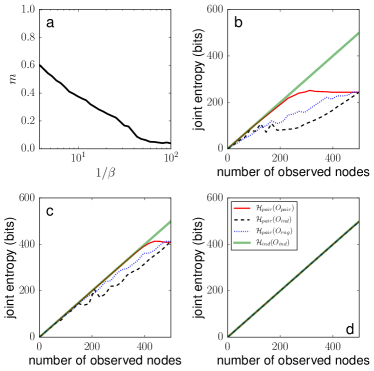
Figure 1: Ising model on the US air transportation network. a) Magnetization $m$ as a function of the temperature $1/\beta$. b) Joint entropy of the observed set as a function of the set size. Here $1/\beta=1$. Sampling techniques considered are: i) MES (red full line); ii) MES under the IBMF approximation (black dashed line); iii) random sampling, i.e., nodes are added to the observed set in random order (blue dotted line). For all sampling techniques, joint entropy is measured using the novel approximation. We plot also the joint entropy according to the IBMF approximation for the set $\varmathbb{O}_{ind}$ (thick green line). c) Same as in panel b, but for $1/\beta=15$. d) Same as in panels b, but for $1/\beta=50$.

In Fig. 1 we show results for the Ising model applied to the US air transportation network (size $N=500$) originally considered in  Colizza et al. (2007). The network contains loops, so that our approximation is not exact. We sample configurations reached by the system after a sufficiently long number of iterations of the Metropolis algorithm with fixed value of the temperature $1/\beta$ and external magnetic field $h=1/N$. Every realization is obtained after $1,000\,N$ total spin flips. The phase diagram of the system is presented in Fig. 1a, showing the typical transition from ordered to disordered configurations as the temperature is increased. We first analyze statistical properties of microscopic configurations obtained at $1/\beta=1$ in Fig. 1b. To estimate the unconditional entropy $\mathcal{H}(i)$ of a generic node $i$, and the pairwise conditional entropy $\mathcal{H}(j|i)$ of a generic pair $(i,j)$, we rely on $T=1,000$ sampled configurations. In addition to $\varmathbb{O}_{pair}$and $\varmathbb{O}_{ind}$, we consider also the set of observed nodes $\varmathbb{O}_{rng}$, built by adding nodes in random order. As the figure clearly shows, our approximation generates noticeable improvements with respect to the the IBMF approximation in the computation of the entropy of subsets of the system. This is apparent from the large value of the difference $\mathcal{H}_{ind}(\varmathbb{O}_{ind})-\mathcal{H}_{pair}(\varmathbb{O}_{ind})$. Concerning different sampling strategies, we also see a significant benefit from using our proposed technique over the naive version of MES. $\mathcal{H}_{pair}(\varmathbb{O}_{pair})$ grows much quicker than $\mathcal{H}_{pair}(\varmathbb{O}_{ind})$, and saturates at the maximum value after about $200$ nodes are observed. This is an indication that the entire uncertainty of the system can be explained by looking at a fraction of the nodes in the network only. On the contrary, $\mathcal{H}_{pair}(\varmathbb{O}_{ind})$ behaves very similarly to, if not worse than, $\mathcal{H}_{pair}(\varmathbb{O}_{rng})$ testifying that the naive MES strategy is not effective in this specific system. As the temperature increases (Fig. 1c), the advantage of using our new approximation in place of the IBMF approximation becomes less apparent. At the same time, the benefit of using our greedy MES strategy compared to the naive version becomes less evident. For very large temperatures, all curves become identical (Fig. 1d).

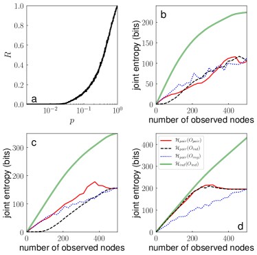
Figure 2: Independent cascade model on the US air transportation network. a) Relative size of the outbreak $R$ as a function of the infection probability $p$. Panels b, c, and refer respectively to $p=0.1$, $p=0.2$, and $p=0.5$. The description of the curves in these panels is identical to one of the curves appearing in Fig. 1.

In Fig. 2, we study the IC model applied to the same real-world network. We focus on microscopic configurations corresponding to the final stage of the dynamics, where nodes are either in the susceptible or recovered state. The initial condition of the dynamics is given by all nodes in the susceptible state, except for a single randomly chosen seed in the infected state. Infections propagate along each active edge with probability $p$. For every value of $p$, we consider $T=100,000$ sampled configurations. In the IC model on a loopy graph, both assumptions at the basis of our approach are violated. Nonetheless, the results reveal that our approximation represents a significant improvement over the basic IBMF approximation. First, we are able to provide estimates of the entropy of the system that are radically smaller, showing that pairwise correlations among variables are particularly significant in the system. Second, we are able to construct sets of observed nodes that are more representative for system uncertainty than those obtained by using the other sampling strategies.

To further strengthen our message, in the SM we include a comparison of the performance between our greedy algorithm for MES and other selection strategies: (i) degree centrality sampling, where nodes are added in decreasing (increasing) order based on their degree; (ii) closeness centrality sampling, the same as (i) but with node ranking based on closeness centrality. These strategies are chosen to test the performance of centrality-based metrics that rely on topological properties only. The most significant difference between them is that degree is a local metric, whereas closeness is global. We find that topological heuristics are not always reliable sampling strategies, and that their effectiveness is seriously affected by the underlying network structure and/or the parameter values of the stochastic models. Further in the SM, we study analytically the behavior of the IC model in star networks and show that the choice of the best nodes to observe is highly sensitive not only to the parameter of the model, but also to the initial configuration of the stochastic dynamical process.

In summary, we introduce an algorithm to approximate the conditional entropy of a sample of nodes in a complex network. The algorithm relies on the sparsity of the graph to simplify computations otherwise unfeasible. Although the algorithm allows us to compute the conditional entropy of arbitrary node sets, it finds a particularly interesting application in the greedy approximation of the so-called MES principle. This principle corresponds to the optimal reduction of uncertainty of a stochastic process taking place on a network. Combining our algorithm with machine learning methods to create active supervised learning approaches is a potentially interesting direction for future investigation. Other extensions worth of consideration are also the generalization of our algorithm to devise computationally feasible selection strategies based on other information-theoretic principles, as for example the maximization of the mutual information rather than entropy.

in 1,…,40 See pages \x, of SM_may18.pdf