Markov Chain Lifting and Distributed ADMM

Abstract

The time to converge to the steady state of a finite Markov chain can be greatly reduced by a lifting operation, which creates a new Markov chain on an expanded state space. For a class of quadratic objectives, we show an analogous behavior where a distributed ADMM algorithm can be seen as a lifting of Gradient Descent algorithm. This provides a deep insight for its faster convergence rate under optimal parameter tuning. We conjecture that this gain is always present, as opposed to the lifting of a Markov chain which sometimes only provides a marginal speedup.

I Introduction

Let $\mathcal{M}$ and $\hat{\mathcal{M}}$ be two finite Markov chains with states $\mathcal{V}$ and $\hat{\mathcal{V}}$, of sizes $|\mathcal{V}|<|\hat{\mathcal{V}}|$, and with transition matrices $M$ and $\hat{M}$, respectively. Let their stationary distributions be $\bm{\pi}$ and $\hat{\bm{\pi}}$. In some cases it is possible to use $\hat{\mathcal{M}}$ to sample from the stationary distribution of $\mathcal{M}$. A formal set of conditions under which this happen is known as lifting. We say that $\hat{\mathcal{M}}$ is a lifting of $\mathcal{M}$ if there is a row stochastic matrix $S\in\mathbb{R}^{|\hat{\mathcal{V}}|\times|\mathcal{V}|}$ with elements $S_{ij}\in\{0,1\}$ and a single nonvanishing element per line, where $\bm{1}_{|\mathcal{V}|}=S^{\top}\bm{1}_{|\hat{\mathcal{V}}|}$, and $\bm{1}_{n}$ is the all-ones $n$-dimensional vector, such that

$$\bm{\pi}=S^{\top}\hat{\bm{\pi}},\qquad D_{\bm{\pi}}M=S^{\top}D_{\hat{\bm{\pi}}}\hat{M}S.$$ (1)

We denote ${S}^{\top}$ the transpose of $S$, and for any vector $\bm{v}\in\mathbb{R}^{n}$, $D_{\bm{v}}=\operatorname{diag}(v_{1},\dots,v_{n})$. Intuitively, $\hat{\mathcal{M}}$ contains copies of the states of $\mathcal{M}$ and transition probabilities between the extended sates $\hat{\mathcal{V}}$ such that it is possible to collapse $\hat{\mathcal{M}}$ onto $\mathcal{M}$. This is the meaning of relation (1). See Fig. 1 for an illustration. (We refer to chen1999lifting for more details on Markov chain lifting.)

The mixing time $\mathcal{H}$ is a measure of the time it takes for the distribution of a Markov chain $\mathcal{M}$ to approach stationarity. We follow the definitions of chen1999lifting but, up to multiplicative factors and slightly loser bounds, the reader can think of

$$\mathcal{H}=\min\{t:\max_{\{i,\bm{p}^{0}\}}|p^{t}_{i}-\pi_{i}|<1/4\},$$ (2)

where $p^{t}_{i}$ is the probability of being on state $i$ after $t$ steps, starting from the initial distribution $\bm{p}^{0}$. Lifting is particularly useful when the mixing time $\hat{\mathcal{H}}$ of the lifted chain is much smaller than $\mathcal{H}$. There are several examples where $\hat{\mathcal{H}}\approx C\sqrt{\mathcal{H}}$, for some constant $C\in(0,1)$ which depends only on $\bm{\pi}$. However, there is a limit on how much speedup can be achieved. If $\mathcal{M}$ is irreducible, then $\hat{\mathcal{H}}\geq C\sqrt{\mathcal{H}}$. If $\mathcal{M}$ and $\hat{\mathcal{M}}$ are reversible, then the limitation is even stronger, $\hat{\mathcal{H}}\geq C\mathcal{H}$.

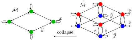
Figure 1: The base Markov chain $\mathcal{M}$ over the cycle graph $C_{4}$ and its lifted Markov chain $\hat{\mathcal{M}}$ with duplicate states. Each state in $\mathcal{V}$ (green nodes) is expanded into two states in $\hat{\mathcal{V}}$ (blue and red nodes above each other).

Consider the undirected and connected graph $\mathcal{G}=(\mathcal{V},\mathcal{E})$, with vertex set $\mathcal{V}$ and edge set $\mathcal{E}$. Let $\bm{z}\in\mathbb{R}^{|\mathcal{V}|}$ with components $z_{i}$, and consider the quadratic problem

$$\min_{\bm{z}\in\mathbb{R}^{|\mathcal{V}|}}\Big{\{}f(\bm{z})=\dfrac{1}{2}\sum_{(i,j)\in\mathcal{E}}q_{ij}(z_{i}-z_{j})^{2}\Big{\}}.$$ (3)

We also write $q_{ij}=q_{e}$ for $e=(i,j)\in\mathcal{E}$. There is a connection between solving (3) by Gradient Descent (GD) algorithm and the evolution of a Markov chain. To see this, consider $q_{e}=1$ for simplicity. The GD iteration with step-size $\alpha>0$ is given by

$$\bm{z}^{t+1}=\left(I-\alpha\nabla f\right)\bm{z}^{t}=\left(I-\alpha D_{\bm{d}}(I-W)\right)\bm{z}^{t}$$ (4)

where $W=D_{\bm{d}}^{-1}A$ is the transition matrix of a random walk on $\mathcal{G}$, $A$ is the adjacency matrix, and $D_{\bm{d}}$ is the degree matrix, where $\bm{d}=\operatorname{diag}(d_{1},\dotsc,d_{|\mathcal{V}|})$.

This connection is specially clear for $d$-regular graphs. Choosing $\alpha=1/d$, equation (4) simplifies to $\bm{z}^{t+1}=W\bm{z}^{t}$. In particular, the convergence rate of GD is determined by the spectrum of $W$, which is connected to the mixing time of $\mathcal{M}$. More precisely, when $W$ is irreducible and aperiodic, and denoting $\lambda_{2}(W)$ its second largest eigenvalue in absolute value, the mixing time of the Markov chain and the convergence time of GD are both equal to

$$\mathcal{H}=\dfrac{C}{\log(1/|\lambda_{2}|)}\approx\dfrac{C}{1-|\lambda_{2}|}$$ (5)

where the constant $C$ comes from the tolerance error, which in (2) is $1/4$. In the above approximation we assumed $\lambda_{2}\approx 1$. Therefore, at least for GD, we can use the theory of Markov chains to analyze the convergence rate when solving optimization problems. For this example, and whenever there is linear convergence, the convergence rate $\tau$ and the convergence time $\mathcal{H}$ are related by $\tau^{\mathcal{H}}=\Theta(1)$. For an introduction on Markov chains, mixing times, and transition matrix eigenvalues, we refer the reader to Norris .

The main goal of this paper is to extend the above connection to the over-relaxed Alternating Direction Method of Multipliers (ADMM) algorithm, and the concept of lifting will play an important role. Specifically, for problem (3), we show that a distributed implementation of over-relaxed ADMM can be seen as a lifting of GD, in the same way that $\hat{\mathcal{M}}$ is a lifting of the Markov chain $\mathcal{M}$. More precisely, there is a matrix $M_{A}$ with stationary vector $v_{A}$ associated to distributed ADMM, and a matrix $M_{G}$ with stationary vector $v_{G}$ associated to GD, such that relation (1) is satisfied. This duality is summarized in Fig. 2. In some cases, $M_{A}$ might have a few negative entries preventing it from being the transition matrix of a Markov chain. However, it always satisfies all the other properties of Markov matrices.

As explained in the example preceding (5), the convergence time of an algorithm can be related to the mixing time of a Markov chain. Let $\mathcal{H}_{A}$ be the convergence time of ADMM, and $\mathcal{H}_{G}$ the convergence time of GD. The lifting relation between both algorithms strongly suggest that, for problem (3) and optimally tuned parameters, ADMM is always faster than GD. Since lifting can speed mixing times of Markov chains up to a square root factor, we conjecture that the optimal convergence times $\mathcal{H}^{\star}_{A}$ and $\mathcal{H}^{\star}_{G}$ are related as

$$\mathcal{H}^{*}_{A}\leq C\sqrt{\mathcal{H}^{*}_{G}},$$ (6)

where $C>0$ is a universal constant. Moreover, we conjecture that (6) holds for any connected graph $\mathcal{G}$. Note that (6) is much stronger than the analogous relation for lifted of Markov chains, where for some graphs, e.g. with low conductance, the gain is marginal.

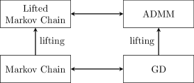
Figure 2: GD is the analogue of a Markov chain, while distributed ADMM is the analogue of a lifted version of this Markov chain, which mixes faster.

The outline of this paper is the following. After mentioning related works in Section II, we state our main results in Section III, which shows that distributed implementations of over-relaxed ADMM and GD obey the lifting relation (1). The proofs can be found in the Appendix. In Section IV we support conjecture (6) with numerical evidence. We present our final remarks in Section V.

II Related Work and an Open Problem

We state conjecture (6) for the relatively simple problem (3), but, to the best of our knowledge, it cannot be resolved through the existing literature. We compare the exact asymptotic convergence rates after optimal tuning of ADMM and GD, while the majority of previous papers focus on upper bounding the global convergence rate of ADMM and, at best, optimize such an upper bound.

Furthermore, to obtain linear convergence, strong convexity is usually assumed shi2014linear , which does not hold for problem (3). Most results not requiring strong convexity focus on the convergence rate of the objective function, as opposed to this paper which focus on the convergence rate of the variables; see davis2014convergence for example.

Few papers consider a consensus problem with an objective function different than (3). For instance, erseghe2011fast considers $f(\bm{z})=\sum_{i\in\mathcal{V}}\sum\|z_{i}-c_{i}\|^{2}$, subject to $z_{i}=z_{j}$ if $(i,j)\in\mathcal{E}$, where $c_{i}>0$ are constants. This problem is strongly convex and does not reduce to (3), and vice-versa. Other branch of research consider $f(\bm{z})=\sum_{i}f_{i}(\bm{z})$ with ADMM iterations that are agnostic to whether or not $f_{i}(\bm{z})$ depends on a subset of the components of $\bm{z}$; see wei2012distributed and references therein. These are in contrast with our setting where decentralized ADMM is a message-passing algorithm Bento1 , and the messages between agents $i$ and $j$ are only associated to the variables shared by functions $f_{i}$ and $f_{j}$.

For quadratic problems, there are explicit results on the convergence rate and optimal parameters of ADMM teixeira2013optimal ; ghadimi2015optimal ; iutzeler2016explicit . However, their assumptions do not hold for the non strongly convex distributed problem considered in this paper. Moreover, there are very few results comparing the optimal convergence rate of ADMM as a function of the optimal convergence rate of GD. For a centralized setting, an explicit comparison is provided in FrancaBento , but it assumes strong convexity.

Finally, and most importantly, there is no prior result connecting GD and ADMM to lifted Markov chains. Lifted Markov chains were previously employed to speedup convergence time of distributed averaging and gossip algorithms jung2007fast ; li2010location ; jung2010distributed , but these do not involve ADMM algorithm.

III ADMM as a Lifting of Gradient Descent

We now show that the lifting relation (1) holds when distributed implementations of over-relaxed ADMM and GD are applied to problem (3) defined over the graph $\mathcal{G}=(\mathcal{V},\mathcal{E})$.

Let us introduce the extended set of variables $\bm{x}\in\mathbb{R}^{|\hat{\mathcal{E}|}}$, where

$$\hat{\mathcal{E}}=\{(e,i):e\in\mathcal{E},\,i\in e,\,\text{and}\,i\in\mathcal{V}\}.$$ (7)

Note that $|\hat{\mathcal{E}}|=2|\mathcal{E}|$. Each component of $\bm{x}$ is indexed by a pair $(e,i)\in\hat{\mathcal{E}}$. For simplicity we denote $e_{i}=(e,i)$. We can now write (3) as

$$\min_{\bm{x},\bm{z}}\Big{\{}f({\bm{x}})=\dfrac{1}{2}\sum_{e=(i,j)\in\mathcal{E}}q_{e}(x_{e_{i}}-x_{e_{j}})^{2}\Big{\}}$$ (8)

subject to $x_{e_{i}}=z_{i}$, $x_{e_{j}}=z_{j}$, for all $e=(i,j)\in\mathcal{E}$. The new variables are defined according to the following diagram:

Notice that we can also write ${f}(\bm{x})=\tfrac{1}{2}{\bm{x}}^{\top}Q\bm{x}$ where $Q$ is block diagonal, one block per edge $e=(i,j)$, in the form $Q_{e}=q_{e}\left(\begin{smallmatrix}+1&-1\\ -1&+1\end{smallmatrix}\right)$. Let us define the matrix $S\in\mathbb{R}^{|\hat{\mathcal{E}}|\times|\mathcal{V}|}$ with components

$$S_{e_{i},i}=S_{e_{j},j}=\begin{cases}1&\mbox{if $e=(i,j)\in\mathcal{E}$,}\\ 0&\mbox{otherwise.}\end{cases}$$ (9)

The distributed over-relaxed ADMM is a first order method that operates on five variables: $\bm{x}$ and $\bm{z}$ defined above, and also $\bm{u}$, $\bm{m}$ and $\bm{n}$ introduced below. It depends on the relaxation parameter $\gamma\in(0,2)$, and several penalty parameters $\bm{\rho}\in\mathbb{R}^{|\hat{\mathcal{E}}|}$. The components of $\bm{\rho}$ are $\rho_{e_{i}}>0$ for $e_{i}\in\hat{\mathcal{E}}$; see FrancaBento ; Bento1 and also Bento2 for details on multiple $\rho$’s. We can now write ADMM iterations as

$$\bm{x}^{t+1} =A\bm{n}^{t},$$ (10)

$$\bm{m}^{t+1} =\gamma\bm{x}^{t+1}+\bm{u}^{t},$$

$$\bm{s}^{t+1} =(1-\gamma)\bm{s}^{t}+B\bm{m}^{t+1},$$

$$\bm{u}^{t+1} =\bm{u}^{t}+\gamma\bm{x}^{t+1}+(1-\gamma)\bm{s}^{t}-\bm{s}^{t+1},$$

$$\bm{n}^{t+1} =\bm{s}^{t+1}-\bm{u}^{t+1},$$

where $\bm{s}^{t}=S\bm{z}^{t}$, $B=S(S^{\top}D_{\bm{\rho}}S)^{-1}S^{\top}D_{\bm{\rho}}$, and $A=(I+D^{-1}_{\bm{\rho}}Q)^{-1}$. The next result shows that these iterations are equivalent to a linear system in $|\hat{\mathcal{E}}|$ dimensions. (The proofs of the following results are in the Appendix.)

Theorem 1 (Linear Evolution of ADMM).

Iterations (10) are equivalent to

$$\bm{n}^{t+1}=T_{A}\,\bm{n}^{t},\qquad T_{A}=I-\gamma(A+B-2BA),$$ (11)

with $\bm{s}^{t}=B\bm{n}^{t}$ and $\bm{u}^{t}=-(I-B)\bm{n}^{t}$. All the variables of ADMM depend only on $\bm{n}^{t}$.

We can also write GD update $\bm{z}^{t+1}=(I-\alpha\nabla f)\bm{z}^{t}$ to problem (3) as

$$\bm{z}^{t+1}=T_{G}\bm{z}^{t},\qquad T_{G}=I-\alpha S^{\top}QS.$$ (12)

In the following, we establish lifting relations between distributed ADMM and GD in terms of matrices $M_{A}$ and $M_{G}$, which are very closely related but not necessarily equal to $T_{A}$ and $T_{G}$. They are defined as

$$M_{G} =(I-D_{G})^{-1}(T_{G}-D_{G}),$$ (13)

$$M_{A} =(I-D_{A})^{-1}(T_{A}-D_{A}),$$ (14)

where $D_{G}\neq I$ and $D_{A}\neq I$ are, for the moment, arbitrary diagonal matrices. Let us also introduce the vectors

$$\bm{v}_{G} =(I-D_{G})\bm{1},$$ (15)

$$\bm{v}_{A} =(I-D_{A})\bm{\rho}.$$ (16)

As shown below, these matrices and vectors satisfy relation (1). Moreover, $M_{G}$ can be interpreted as a probability transition matrix, and the rows of $M_{A}$ sum up to one. We only lack the strict non-negativity of $M_{A}$, which in general is not a probability transition matrix. Thus, in general, we do not have a lifting between Markov chains, however, we still have lifting in the sense that $M_{A}$ can be collapsed onto $M_{G}$ according to (1).

Theorem 2.

For $(D_{G})_{ii}<1$ and sufficiently small $\alpha$, $M_{G}$ in (13) is a doubly stochastic matrix.

Lemma 3.

The rows of $M_{G}$ and $M_{A}$ sum up to one, i.e. $M_{G}\bm{1}=\bm{1}$ and $M_{A}\bm{1}=\bm{1}$. Moreover, ${\bm{v}}_{G}^{\top}M_{G}={\bm{v}}_{G}^{\top}$ and $\bm{v}_{A}^{\top}M_{A}=\bm{v}_{A}^{\top}$. These properties are shared with Markov matrices.

Theorem 4 (ADMM as a Lifting of GD).

$M_{A}$ and $M_{G}$ defined in (13) and (14) satisfy relation (1), namely,

$$\bm{v}_{G}=S^{\top}\bm{v}_{A},\qquad D_{\bm{v}_{G}}M_{G}=S^{\top}D_{\bm{v}_{A}}M_{A}S,$$ (17)

provided $D_{G}$, $D_{A}$, $\alpha$, $\gamma$, and $\bm{\rho}$ are related according to

$$S^{\top}D_{\bm{\rho}}(I-D_{A})S=I-D_{G},$$ (18)

$$\alpha=\dfrac{\gamma\,q_{e}\rho_{e_{i},i}\,\rho_{e_{j},j}}{\rho_{e_{i},i}\,\rho_{e_{j},j}+q_{e}\left(\rho_{e_{i},i}+\rho_{e_{j},j}\right)},$$ (19)

for all $e=(i,j)\in\mathcal{E}$. Equation (19) restricts the components of $\bm{\rho}$, and (17) is an equation for $D_{A}$ and $D_{G}$.

Theorem 5 (Negative Probabilities).

There exists a graph $\mathcal{G}$ such that, for any diagonal matrix $D_{A}$, $\bm{\rho}$ and $\gamma$, the matrix $M_{A}$ has at least one negative entry. Thus, in general, $M_{A}$ is not a probability transition matrix.

For concreteness, let us consider some explicit examples illustrating Theorem 4.

Regular Graphs.

Let us consider the solution to equations (18) and (19) for $d$-regular graphs. Fix $q_{e}=1$ and $\bm{\rho}=\rho\bm{1}$ for simplicity. Equation (18) is satisfied with

$$D_{A}=(1-(\rho|\hat{\mathcal{E}}|)^{-1})I,\qquad D_{G}=(1-|\mathcal{V}|^{-1})I,$$ (20)

since $d|\mathcal{V}|=|\hat{\mathcal{E}}|=2|\mathcal{E}|$, while (19) requires

$$\alpha=\dfrac{\gamma\rho}{2+\rho}.$$ (21)

Notice that $(D_{G})_{ii}<1$ for all $i$, so choosing $\gamma$ or $\rho$ small enough we can make $M_{G}$ positive. Moreover, the components of (15) and (16) are non-negative and sum up to one, i.e. ${\bm{v}}^{\top}_{G}{\bm{1}}={\bm{v}}^{\top}_{A}{\bm{1}}=1$, thus these vectors are stationary probability distributions of $M_{G}$ and $M_{A}$.

Cycle Graph.

Consider solving (3) over the $4$-node cycle graph $\mathcal{G}=C_{4}$ shown in Fig. 1. By direct computation and upon using (20) we obtain

$$M_{G}=\begin{pmatrix}x&y&0&y\\ y&x&y&0\\ 0&y&x&y\\ y&0&y&x\\ \end{pmatrix},\qquad M_{A}=\begin{pmatrix}\hat{x}&0&0&0&0&0&\hat{y}&\hat{z}\\ 0&\hat{x}&\hat{z}&\hat{y}&0&0&0&0\\ \hat{y}&\hat{z}&\hat{x}&0&0&0&0&0\\ 0&0&0&\hat{x}&\hat{z}&\hat{y}&0&0\\ 0&0&\hat{y}&\hat{z}&\hat{x}&0&0&0\\ 0&0&\hat{y}&0&0&\hat{x}&\hat{z}&\hat{y}\\ 0&0&0&0&\hat{y}&\hat{z}&\hat{x}&0\\ \hat{z}&\hat{y}&0&0&0&0&0&\hat{x}\end{pmatrix},$$ (22)

where the probabilities of $M_{G}$ are given by $x=1-8\alpha$ and $x+2y=1$, and the probabilities of $M_{A}$ are $\hat{x}=1-4\gamma\rho$, $\hat{y}=8\gamma\rho/(2+\rho)$ and $\hat{x}+\hat{y}+\hat{z}=1$. The stationary probability vectors are $\bm{\pi}=\tfrac{1}{4}\bm{1}$ and $\hat{\bm{\pi}}=\tfrac{1}{8}\bm{1}$. Now (17) holds provided the parameters are related as (21). Moreover, in this particular case the matrix $M_{A}$ is strictly non-negative, thus ADMM is a lifting of GD in the Markov chain sense.

Based on the above theorems we propose conjecture (6). The convergence rate $\tau$ is related to the convergence time, for instance $\mathcal{H}\sim(1-\tau)^{-1}$ if $\tau\approx 1$. Thus, let $\tau_{G}^{\star}$ and $\tau_{A}^{\star}$ be the optimal convergence rates of GD and ADMM, respectively. Then, at least for objective (3), and for any $\mathcal{G}$, we conjecture that there is some universal constant $C>0$ such that

$$1-\tau_{A}^{\star}\geq C\sqrt{1-\tau_{G}^{\star}}.$$ (23)

IV Numerical evidence

For many graphs, we observe very few negative entries in $M_{A}$, which can be further reduced by adjusting the parameters $\bm{\rho}$ and $\gamma$. Nonetheless, in general, the lack of strict non-negativity of $M_{A}$ prevents us from directly applying the theory of lifted Markov chains to prove (23). However, there is compelling numerical evidence to (23) as we now show.

Consider a sequence of graphs $\{\mathcal{G}_{n}\}$, where $n=|\mathcal{V}|$, such that $\tau^{\star}_{G}\to 1$ and $\tau^{\star}_{A}\to 1$ as $n\to\infty$. Denote $\mathcal{R}_{G}(n)=(1-\tau_{G}^{\star})^{-1}$ and $\mathcal{R}_{A}(n)=(1-\tau_{A}^{\star})^{-1}$. We look for the smallest $\beta$ such that $\mathcal{R}_{A}(n)\leq C\,\mathcal{R}_{G}(n)^{\beta}$, for some $C>0$, and all large enough $n$. If (23) was false, there would exist sequences $\{\mathcal{G}_{n}\}$ for which $\beta>1/2$. For instance, if $\{\mathcal{G}_{n}\}$ have low conductance it is well-known that lifting does not speedup the mixing time and we could find $\beta=1$.

To numerically find $\beta$, we plot

$$\hat{\beta}_{1}=\dfrac{\log\mathcal{R}_{A}(n)}{\log\mathcal{R}_{G}(n)}\quad\mbox{and}\quad\hat{\beta}_{2}=\dfrac{\mathcal{R}_{G}(n)}{\mathcal{R}_{A}(n)}\,\dfrac{\Delta\mathcal{R}_{A}(n)}{\Delta\mathcal{R}_{G}(n)}$$ (24)

against $n$, where $\Delta h(n)=h(n+1)-h(n)$ for any function $h(n)$. The idea behind this is very simple. Let $f(x)=Cg(x)^{\beta}$, and $f,g\to\infty$ as $x\to\infty$. Then, ${\log f}/{\log g}\to\beta$ and also ${\partial_{x}\log f}/{\partial_{x}\log g}={(g\,\partial_{x}f)}/{(f\,\partial_{x}g)}\to\beta$ as $x\to\infty$. Thus, we analyze (24) which are their discrete analogue. Given a graph $\mathcal{G}_{n}$, from (12) and (11) we numerically compute $\tau=\max_{j}\{|\lambda_{j}(T)|:|\lambda_{j}(T)|<1\}$. The optimal convergence rates are thus given by $\tau_{G}^{\star}=\min_{\alpha}\tau_{G}$ and $\tau_{A}^{\star}=\min_{\{\gamma,\rho\}}\tau_{A}$, where we consider $\bm{\rho}=\rho{\bm{1}}$ with $\rho>0$.

In Fig. 3 we show the three different graphs considered in the numerical analysis contained in the respective plots of Fig. 4. We show the values of (24) versus $n$, and also the curves $\log\mathcal{R}_{A}$ and $\log\mathcal{R}_{G}$ against $n$, which for visualization purposes are scaled by the factor $-0.03$. In Fig. 4a we see that (6), or equivalently (23), holds for the cycle graph $\mathcal{G}=C_{n}$. The same is true for the periodic grid, or torus grid graph $\mathcal{G}=T_{n}$, as shown in Fig. 4b. Surprisingly, as shown in Fig. 4c, we get the same square root speedup for a barbell graph, whose random walk is known to not speedup via lifting. We find similar behavior for several other graphs but we omit these results due to the lack of space.

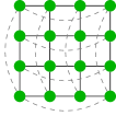
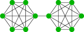
Figure 3: We consider the following graphs for numerical analysis. (a) Cycle graph, $\mathcal{G}=C_{n}$. (b) Torus or periodic grid graph, $\mathcal{G}=T_{n}=C_{\sqrt{n}}\times C_{\sqrt{n}}$. (c) Barbel graph, obtained by connecting two complete graphs $K_{n}$ by a bridge.

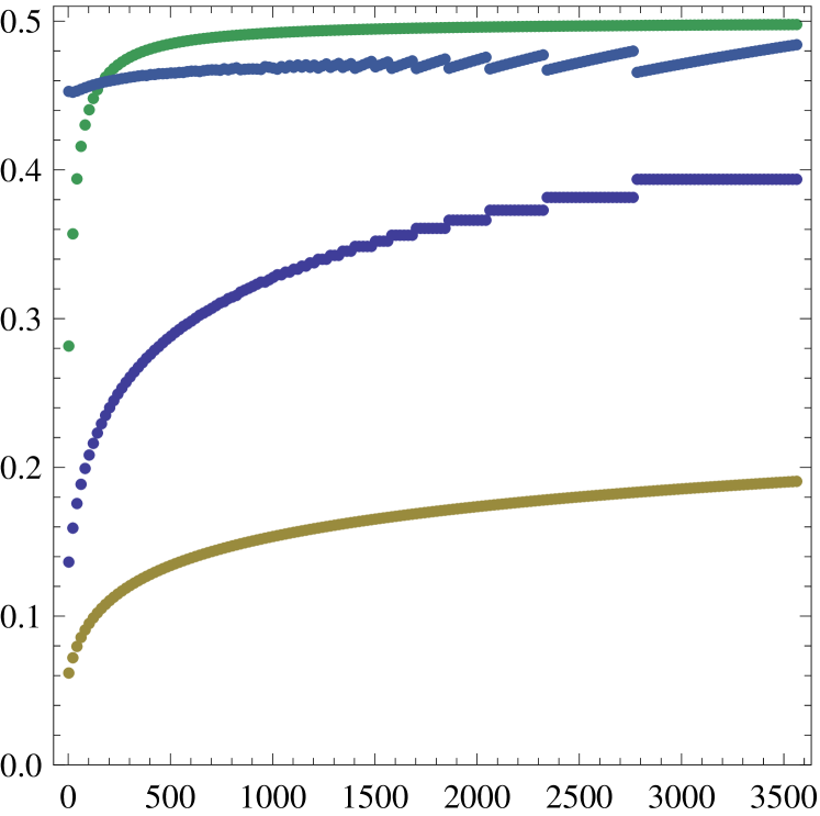
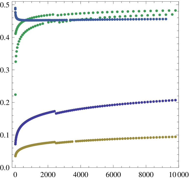
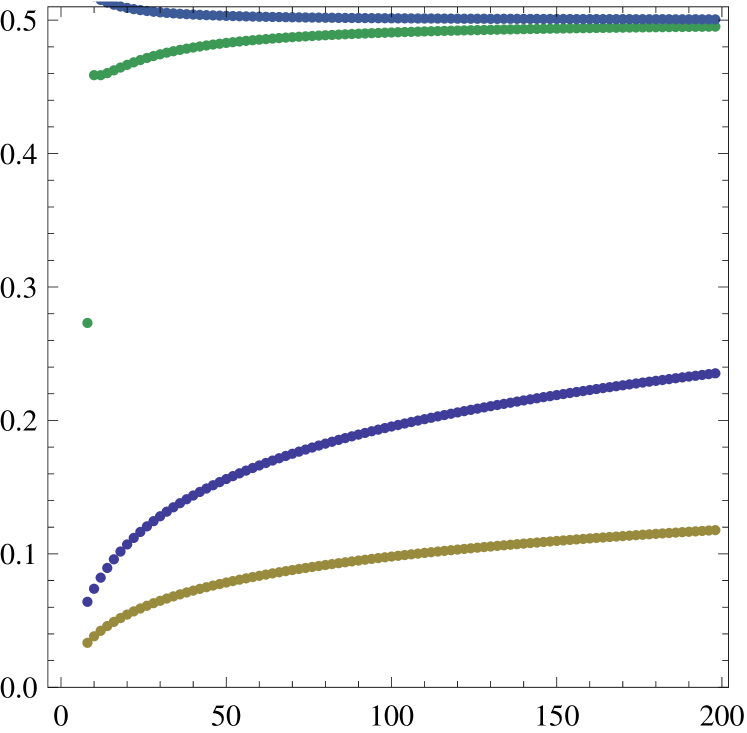
Figure 4: Plot of (24) versus $n$, and also $\log\mathcal{R}_{A}$ and $\log\mathcal{R}_{G}$ versus $n$, scaled by $-0.03$ for visualization purposes only. The sequence of graphs $\{\mathcal{G}_{n}\}$ in each plot are of the types indicated in Fig. 3, in the same respective order. Notice that $\hat{\beta}_{1},\hat{\beta}_{2}\leq 1/2$, and $\hat{\beta}_{1}$ and $\hat{\beta_{2}}$ gets very close to $1/2$ for large $n$. (a) Cycle graph. (b) Torus grid graph. The two green curves occur because odd and even $n$ behave differently. (c) Barbell graph. A Markov chain over this graph does not speedup via lifting, however, (23) still holds.

V Conclusion

For a class of quadratic problems (3) we established a duality between lifted Markov chains and two important distributed optimization algorithms, GD and over-relaxed ADMM; see Fig. 2. We proved that precisely the same relation defining lifting of Markov chains (1), is satisfied between ADMM and GD. This is the content of Theorem 4. Although the lifting relation holds, in general, we cannot guarantee that the matrix $M_{A}$ associated to ADMM is a probability transition matrix, since it might have a few negative entries. Therefore, in general, Theorem 4 is not a Markov chain lifting, but it is a lifting in a graph theoretical sense.

These negative entries actually make this parallel even more interesting since (6), or equivalently (23), do not violate theorems of lifted Markov chains where the square root improvement is a lower bound, thus the best possible, and in (6) it is an upper bound. For graphs with low conductance, the speedup given by Markov chain lifting is negligible. On the other hand, the lifting between ADMM and GD seems to always give the best possible speedup achieved by Markov chains, even for graphs with low conductance. This is numerically confirmed in Fig. 4c.

Due to the strong analogy with lifted Markov chains and numerical evidence, we conjectured the upper bound (6), or (23), which was well supported numerically. However, its formal explanation remains open.

Finally, although we considered a simple class of quadratic objectives, when close to the minimum the leading order term of more general convex functions is usually quadratic. In the cases where the dominant term is close to the form (3), the results presented in this paper should still hold. An attempt to prove our conjecture (23) is under investigation.

Appendix A Proof of Main Results

In the main part of the paper we introduced the extended edge set $\hat{\mathcal{E}}$ which essentially duplicates the edges of the original graph, $|\hat{\mathcal{E}}|=2|\mathcal{E}|$. This is the shortest route to state our results concisely but it complicates the notation in the following proofs. Therefore, we first introduce the notion of a factor graph for problem (3).

A.1 Factor Graph

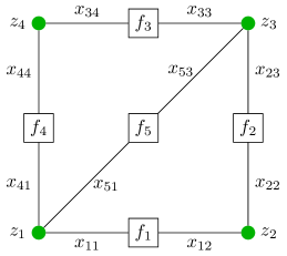
Figure 5: Example of a factor graph $\bar{\mathcal{G}}$ for problem (3), and (8), where $\mathcal{G}$ is the complete graph $K_{4}$ with one edge removed.

The factor graph $\bar{\mathcal{G}}=(\bar{\mathcal{F}},\bar{\mathcal{V}},\bar{\mathcal{E}})$ for problem (3) is a bipartite graph that summarizes how different variables are shared across different terms in the objective. This is illustrated in Fig. 5, where for this case (3) is given by

$$\begin{split}f(\bm{z})&=q^{1}(z_{1}-z_{2})^{2}+q^{2}(z_{2}-z_{3})^{2}+q^{3}(z_{3}-z_{4})^{2}\\ &\qquad+q^{4}(z_{4}-z_{1})^{2}+q^{5}(z_{4}-z_{2})^{2}\end{split}$$ (25)

while (8) is given by

$$\begin{split}&f(\bm{x})=q^{1}(x_{12}-x_{11})^{2}+q^{2}(x_{23}-x_{22})^{2}\\ &+q^{3}(x_{34}-x_{33})^{2}+q^{4}(x_{41}-x_{44})^{2}+q^{5}(x_{45}-x_{52})^{2}\end{split}$$ (26)

where $x_{11}=x_{41}$, $x_{12}=x_{22}$, $x_{23}=x_{33}$, and $x_{44}=x_{34}$.

The factor graph $\bar{\mathcal{G}}$ has two sets of vertices, $\bar{\mathcal{F}}$ and $\bar{\mathcal{V}}$. The circles in Fig. 5 represent the nodes in $\bar{\mathcal{V}}=\mathcal{V}$, and the squares represent the nodes in $\bar{\mathcal{F}}=\mathcal{E}$, where $\mathcal{G}=(\mathcal{V},\mathcal{E})$ is the original graph. Note that each $a\in\bar{\mathcal{F}}$ is uniquely associated to one edge $e\in\mathcal{E}$, and uniquely associated to one term in the sum of the objective. In equation (8) we referred to each term as $f_{e}=q_{e}(x_{e_{i}}-x_{e_{j}})^{2}$, but now we refer to it by $f_{a}$. With a slightly abuse of notation we indiscriminately write $a\in\bar{\mathcal{F}}$ or $f_{a}\in\bar{\mathcal{F}}$. Each node $b\in\bar{\mathcal{V}}$ is uniquely associated to one node $i\in\mathcal{V}$, and uniquely associated to one component of $\bm{z}$. Before we referred to this variable by $z_{i}$, but now we refer to it by $z_{b}$, and indiscriminately write $b\in\bar{\mathcal{F}}$ or $z_{b}\in\bar{\mathcal{F}}$. Each edge $(a,b)\in\bar{\mathcal{E}}$ must have $a\in\bar{\mathcal{F}}$ and $b\in\bar{\mathcal{V}}$, and its existence implies that the function $f_{a}$ depends on variable $z_{b}$. Moreover, each edge $(a,b)\in\bar{\mathcal{E}}$ is also uniquely associated to one component of $\bm{x}$ in the equivalent formulation (8). In particular, if $a\in\bar{\mathcal{E}}$ is associated to $e\in\mathcal{E}$, and $b\in\bar{\mathcal{V}}$ is associated to $i\in\mathcal{V}$, then $(a,b)\in\bar{\mathcal{E}}$ is associated to $x_{e_{i}}$. Here, we denote $x_{e_{i}}$ by $x_{ab}$. Thus, we can think of $\bar{\mathcal{E}}$ as being the same as $\hat{\mathcal{E}}$. Another way of thinking of $\bar{\mathcal{E}}$ and $\bm{x}$ is as follows. If $(a,b)\in\bar{\mathcal{E}}$ then $x_{ab}=z_{b}$ appears as a constraint in (8).

Let us introduce the neighbor set of a given node in $\bar{\mathcal{G}}$. For $a\in\bar{\mathcal{F}}$, the independent variables of $f_{a}$ are in the set

$$N_{a}=\{b\in\bar{\mathcal{V}}:(a,b)\in\bar{\mathcal{G}}\}.$$ (27)

Analogously, for $b\in\bar{\mathcal{V}}$, the functions that depend on $z_{b}$ are in the set

$$N_{b}=\{a\in\bar{\mathcal{F}}:(a,b)\in\bar{\mathcal{G}}\}.$$ (28)

In other words, $N_{\bullet}$ denotes the neighbors of either circle or square nodes in $\bar{\mathcal{G}}$. For $a\in\bar{\mathcal{F}}$ we define

$$I_{a}=\{e\in\bar{\mathcal{E}}:e\text{ is incident on }a\}.$$ (29)

For $b\in\bar{\mathcal{V}}$ we define

$$I_{b}=\{e\in\bar{\mathcal{E}}:e\text{ is incident on }b\}.$$ (30)

If we re-write problem (8) using this new notation, which indexes variables by the position they the take on $\bar{\mathcal{G}}$, the objective function takes the form

$$f(\bm{x})=\dfrac{1}{2}\bm{x}^{\top}Q\bm{x}=\dfrac{1}{2}\sum_{a\in\mathcal{F}}\bm{x}_{a}^{\top}Q^{a}\bm{x}_{a}$$ (31)

where $Q\in\mathbb{R}^{\bar{\mathcal{E}}\times\bar{\mathcal{E}}}$ is block diagonal and each block, now indexed by $a\in\bar{\mathcal{F}}$, takes the form $Q^{a}=q^{a}\left(\begin{smallmatrix}+1&-1\\ -1&+1\end{smallmatrix}\right)$, where $q^{a}>0$, and $\bm{x}_{a}=(x_{ab},x_{ac})^{\top}$ for $(a,b)\in\bar{\mathcal{E}}$ and $(a,c)\in\bar{\mathcal{E}}$. Here, $q^{a}$ is the same as $q_{e}$ in the main text. We also have the constraints $x_{ab}=x_{a^{\prime}b}=z_{b}$ for each $a,a^{\prime}\in N_{b}$ and $b\in\bar{\mathcal{V}}$. The row stochastic matrix $S$ introduced in the ADMM iterations is now expressed as $S\in\mathbb{R}^{|\bar{\mathcal{E}}|\times|\bar{\mathcal{V}}|}$ and has a single $1$ per row such that $S_{eb}=1$ if and only if edge $e\in\bar{\mathcal{E}}$ is incident on $b\in\bar{\mathcal{V}}$. Notice that $S^{\top}S=D_{\bm{d}}$ is the degree matrix of the original graph $\mathcal{G}$.

With this notation at hands, we now proceed to the proofs.

A.2 Proof of Theorem 1

Recall that $B=S(S^{\top}D_{\rho}S)^{-1}S^{\top}D_{\rho}$, thus $B^{2}=B$ is a projection operator, and $B^{\perp}=I-B$ its orthogonal complement. Consider updates (10). Substituting $\bm{x}^{t+1}$ and $\bm{m}^{t+1}$ into the other variables we obtain

$$\begin{pmatrix}I&0&0\\ I&I&0\\ -I&I&I\\ \end{pmatrix}\begin{pmatrix}\bm{s}^{t+1}\\ \bm{u}^{t+1}\\ \bm{n}^{t+1}\end{pmatrix}=\begin{pmatrix}(1-\gamma)I&B&\gamma BA\\ (1-\gamma)I&I&\gamma A\\ 0&0&0\end{pmatrix}\begin{pmatrix}\bm{s}^{t}\\ \bm{u}^{t}\\ \bm{n}^{t}\end{pmatrix}$$

which can be easily inverted yielding

$$\bm{s}^{t+1} =(1-\gamma)\bm{s}^{t}+B\bm{u}^{t}+\gamma BA\bm{n}^{t},$$ (32)

$$\bm{u}^{t+1} =B^{\perp}\bm{u}^{t}+\gamma B^{\perp}A\bm{n}^{t},$$ (33)

$$\bm{n}^{t+1} =(1-\gamma)\bm{s}^{t}+(B-B^{\perp})\bm{u}^{t}+\gamma(B-B^{\perp})A\bm{n}^{t}.$$ (34)

Note the following important relations:

$$B\bm{n}^{t} =\bm{s}^{t}, B^{\perp}\bm{n}^{t} =-\bm{u}^{t},$$ (35)

$$B\bm{s}^{t} =\bm{s}^{t}, B^{\perp}\bm{s}^{t} =0,$$ (36)

$$B^{\perp}\bm{u}^{t} =\bm{u}^{t}, B\bm{u}^{t} =0.$$ (37)

Equation (36) is a simple consequence of the definition of $B$, i.e.

$$B\,\bm{s}^{t}=S(S^{\top}D_{\bm{\rho}}S)^{-1}(S^{\top}D_{\bm{\rho}}S)\bm{z}^{t}=\bm{s}^{t},$$ (38)

which also implies $B^{\perp}\bm{s}^{t}=\bm{0}$. Since $BB^{\perp}=0$, acting with $B$ over (33) implies $B\bm{u}^{t}=\bm{0}$ for every $t$, and also $B^{\perp}\bm{u}^{t}=\bm{u}^{t}$, which shows (37). Now (35) follows from these facts and the own definition $\bm{n}^{t}=\bm{s}^{t}-\bm{u}^{t}$. Finally, applying (35) on (34) we obtain $\bm{n}^{t+1}=T_{A}\bm{n}^{t}$ where $T_{A}=I-\gamma(A+B-2BA)$.

A.3 Proof of Theorem 2

Write $Q=Q^{+}+Q^{-}$ where $Q^{+}$ is diagonal and has only positive entries, and $Q^{-}$ only has off-diagonal and negative entries. First, notice that $(S^{\top}Q^{+}S)$ is also diagonal. Indeed, for $b\in\bar{\mathcal{V}}$ and $c\in\bar{\mathcal{V}}$, $(S^{\top}Q^{+}S)_{bc}=\sum_{e\in\bar{\mathcal{E}}}S_{eb}Q^{+}_{ee}S_{ec}=\delta_{bc}\sum_{e\in I_{b}}Q^{+}_{ee}$ where $\delta$ is the Kronecker delta. By a similar argument, $S^{\top}Q^{-}S$ is off-diagonal. Hence, if $b\neq c$ we have

$$(T_{G})_{bc}=-\alpha\sum_{e\in I_{b}}\sum_{e^{\prime}\in I_{c}}Q^{-}_{ee^{\prime}}\geq 0.$$ (39)

Recall that $M_{G}=(I-D_{G})^{-1}(T_{G}-D_{G})$, where $D_{G}\neq I$ is diagonal. For $M_{G}$ to be non-negative we first impose that $(D_{G})_{bb}<1$ for all $b\in\bar{\mathcal{V}}$. Then, since the off-diagonal elements of $T_{G}$ are automatically positive by (39), we just need to consider the diagonal elements of $T_{G}-D_{G}$. Thus we require that for every $b\in\bar{\mathcal{V}}$,

$$1-\alpha\sum_{e\in I_{b}}Q_{ee}+(D_{G})_{bb}\geq 0.$$ (40)

Denoting $Q_{\textnormal{max}}=\max_{b\in\bar{\mathcal{V}}}\sum_{e\in I_{b}}Q_{ee}$ and $D_{G,\textnormal{min}}$ the smallest element of $D_{G}$, the matrix $M_{G}$ will be non-negative provided $\alpha\leq(1+D_{G,\textnormal{min}})/Q_{\textnormal{max}}$.

Notice that $S\bm{1}_{|\bar{\mathcal{V}}|}=\bm{1}_{|\bar{\mathcal{E}}|}$ and $Q\bm{1}=\bm{0}$. Thus $S^{\top}QS\bm{1}=\bm{0}$, implying $T_{G}\bm{1}=\bm{1}$, and $\bm{1}^{\top}T_{G}=\bm{1}^{\top}$. From this we have $M_{G}\bm{1}=\bm{1}$ and $\bm{1}^{\top}M_{G}=\bm{1}^{\top}$, so all the rows and columns of $M_{G}$ sum up to one.

A.4 Proof of Lemma 3

We proved above that $M_{G}$ is a doubly stochastic matrix. Now let us consider $M_{A}$. Recall the definition of $B=S^{\top}(S^{\top}D_{\bm{\rho}}S)^{-1}S^{\top}D_{\bm{\rho}}$. Note that the action of $B$ on a vector $\bm{v}\in\mathbb{R}^{|\bar{\mathcal{E}}|}$ is to take a weighted average of its components, namely, if $(a,b)\in\bar{\mathcal{E}}$ then

$$(B\bm{v})_{ab}=\dfrac{\sum_{c\in N_{b}}\rho_{cb}v_{cb}}{\sum_{c\in N_{b}}\rho_{cb}}.$$ (41)

Therefore, $B{\bm{1}}={\bm{1}}$. Recall that $Q\bm{1}=\bm{0}$, thus $A{\bm{1}}=\bm{1}$, where $A=(I+D_{\bm{\rho}}^{-1}Q)^{-1}$, which implies $T_{A}\bm{1}=\bm{1}$, and in turn $M_{A}\bm{1}=\bm{1}$. Now the other relations follow trivially.

A.5 Proof of Theorem 4

Due to the block diagonal structure of $Q$ it is possible write $A$ explicitly as

$$A=I-FQ,$$ (42)

where $F$ is a block diagonal matrix with $|\bar{\mathcal{F}}|$ blocks. Each block $F^{a}$, for $a\in\bar{\mathcal{F}}$, is of the form

$$\qquad F^{a}=\dfrac{q^{a}}{\rho_{ab}\rho_{ac}+q^{a}(\rho_{ab}+\rho_{ac})}\begin{pmatrix}\rho_{ac}&0\\ 0&\rho_{ab}\end{pmatrix},$$ (43)

where $b,c\in N_{a}$. Now by the definition of $B$ we have $S^{\top}D_{\bm{\rho}}B=S^{\top}D_{\bm{\rho}}$. Hence,

$$S^{\top}D_{\bm{v}_{A}}M_{A}S =S^{\top}D_{\bm{\rho}}(I-D_{A})S-\gamma S^{\top}D_{\bm{\rho}}FQS,$$ (44)

$$D_{\bm{v}_{G}}M_{G} =(I-D_{G})-\alpha S^{\top}QS.$$ (45)

Equating the first term of (44) to the first term of (45), and also the second terms to each other, on using (42) we obtain

$$S^{\top}D_{\bm{\rho}}(I-D_{A})S=I-D_{G},$$ (46)

$$\alpha=\dfrac{\gamma\,q^{a}\rho_{ab}\rho_{ac}}{\rho_{ab}\rho_{ac}+q^{a}(\rho_{ab}+\rho_{bc})},$$ (47)

where (47) must hold for all $a\in\bar{\mathcal{F}}$ and $b,c\in N_{a}$. This gives the second equality in (17) together with relations (18) and (19). Finally, since diagonal matrices commute, $S^{\top}\bm{v}_{A}=S^{\top}(I-D_{A})D_{\bm{\rho}}S\bm{1}_{|\bar{\mathcal{V}}|}=(I-D_{G})\bm{1}_{|\bar{\mathcal{V}}|}=\bm{v}_{G}$, which gives the first relation in (17).

A.6 Proof of Theorem 5

It suffices to show one example with at least one negative entry. Let $\mathcal{G}$ be the complete graph $K_{4}$ with one edge removed, as shown in Fig. 5. By direct inspection one finds the following sub-matrix of $T_{A}$:

$$T^{(S)}=\begin{pmatrix}(T_{A})_{21}&(T_{A})_{24}\\ (T_{A})_{31}&(T_{A})_{34}\end{pmatrix}$$ (48)

whose elements are explicitly given by

$$(T_{A})_{21} =\tfrac{\gamma\,\rho_{11}(\rho_{12}-\rho_{22})}{(\rho_{12}+\rho_{22})(\rho_{11}+\rho_{12}+\rho_{11}\rho_{12})},$$ (49)

$$(T_{A})_{24} =\tfrac{2\gamma}{(\rho_{12}+\rho_{22})\big{(}1+\rho_{22}^{-1}+\rho_{23}^{-1}\big{)}},$$ (50)

$$(T_{A})_{31} =\tfrac{2\gamma}{(\rho_{12}+\rho_{22})\big{(}1+\rho_{11}^{-1}+\rho_{12}^{-1}\big{)}},$$ (51)

$$(T_{A})_{34} =-\tfrac{\gamma\,\rho_{23}(\rho_{12}-\rho_{22})}{(\rho_{12}+\rho_{22})(\rho_{22}+\rho_{23}+\rho_{22}\rho_{23})}.$$ (52)

First notice that subtracting $D_{A}$ from $T_{A}$ does not affect $T^{(S)}$. Now recall that all components of $\bm{\rho}$ must be strictly positive. The elements (49) and (52) have opposite signs, so one of them is negative. Since (50) and (51) are both positive, one cannot remove the negative entries of an entire row of $T_{A}$ by multiplying $T_{A}$ by the diagonal matrix $(I-D_{A})^{-1}$. Therefore, $M_{A}=(I-D_{A})^{-1}(T_{A}-D_{A})$ has at least one negative entry.

References

- (1) F. Chen, L. Lovász, and L. Pak. Lifting Markov Chains to Speed up Mixing. In Proceedings of the thirty-first annual ACM symposium on Theory of computing, pages 275–281, 1999.
- (2) J. Norris. Markov Chains. Cambridge University Press, Cambridge, 1998.
- (3) W. Shi, Q. Ling, K. Yuan, G. Wu, and W. Yin. On the Linear Convergence of the ADMM in Decentralized Consensus Optimization. IEEE Transactions on Signal Processing, 62(7):1750–1761, 2014.
- (4) D. Davis and W. Yin. Convergence Rate Analysis of Several Splitting Schemes. arXiv preprint arXiv:1406.4834, 2014.
- (5) T. Erseghe, D. Zennaro, E. Dall’Anese, and L. Vangelista. Fast Consensus by the Alternating Direction Multipliers Method. IEEE Transactions on Signal Processing, 59(11):5523–5537, 2011.
- (6) E. Wei and A. Ozdaglar. Distributed Alternating Direction Method of Multipliers. In 2012 IEEE 51st IEEE Conference on Decision and Control (CDC), pages 5445–5450. IEEE, 2012.
- (7) N. Derbinsky, J. Bento, V. Elser, and J. Yedidia. An Improved Three-Weight Message Passing Algorithm. arXiv:1305.1961v1 [cs.AI], 2013.
- (8) André Teixeira, Euhanna Ghadimi, Iman Shames, Henrik Sandberg, and Mikael Johansson. Optimal Scaling of the ADMM Algorithm for Distributed Quadratic Programming. In 52nd IEEE Conference on Decision and Control, pages 6868–6873. IEEE, 2013.
- (9) E. Ghadimi, A. Teixeira, I. Shames, and M. Johansson. Optimal Parameter Selection for the Alternating Direction Method of Multipliers (ADMM): Quadratic Problems. IEEE Transactions on Automatic Control, 60(3):644–658, 2015.
- (10) F. Iutzeler, P. Bianchi, P. Ciblat, and W. Hachem. Explicit Convergence Rate of a Distributed Alternating Direction Method of Multipliers. IEEE Transactions on Automatic Control, 61(4):892–904, 2016.
- (11) G. França and J. Bento. An Explicit Rate Bound for Over-Relaxed ADMM. In IEEE International Symposium on Information Theory, ISIT 2016, Barcelona, Spain, July 10-15, 2016, pages 2104–2108, 2016.
- (12) K. Jung, D. Shah, and J. Shin. Fast Gossip Through Lifted Markov Chains. In Proc. Allerton Conf. on Comm., Control, and Computing, Urbana-Champaign, IL, 2007.
- (13) W. Li, H. Dai, and Y. Zhang. Location-Aided Fast Distributed Consensus in Wireless Networks. IEEE Transactions on Information Theory, 56(12):6208–6227, 2010.
- (14) K. Jung, D. Shah, and J. Shin. Distributed averaging via lifted markov chains. IEEE Transactions on Information Theory, 56(1):634–647, 2010.
- (15) J. Bento, N. Derbinsky, J. Alonso-Mora, and J. Yedidia. A Message-Passing Algorithm for Multi-Agent Trajectory Planning. In C. J. C. Burges, L. Bottou, M. Welling, Z. Ghahramani, and K. Q. Weinberger, editors, Advances in Neural Information Processing Systems 26, pages 521–529. Curran Associates, Inc., 2013.