Inhomogeneous exponential jump model

Abstract.

We introduce and study the inhomogeneous exponential jump model — an integrable stochastic interacting particle system on the continuous half line evolving in continuous time. An important feature of the system is the presence of arbitrary spatial inhomogeneity on the half line which does not break the integrability. We completely characterize the macroscopic limit shape and asymptotic fluctuations of the height function (= integrated current) in the model. In particular, we explain how the presence of inhomogeneity may lead to macroscopic phase transitions in the limit shape such as shocks or traffic jams. Away from these singularities the asymptotic fluctuations of the height function around its macroscopic limit shape are governed by the GUE Tracy–Widom distribution. A surprising result is that while the limit shape is discontinuous at a traffic jam caused by a macroscopic slowdown in the inhomogeneity, fluctuations on both sides of such a traffic jam still have the GUE Tracy–Widom distribution (but with different non-universal normalizations).

The integrability of the model comes from the fact that it is a degeneration of the inhomogeneous stochastic higher spin six vertex models studied earlier in [BP16]. Our results on fluctuations are obtained via an asymptotic analysis of Fredholm determinantal formulas arising from contour integral expressions for the $q$-moments in the stochastic higher spin six vertex model. We also discuss “product-form” translation invariant stationary distributions of the exponential jump model which lead to an alternative hydrodynamic-type heuristic derivation of the macroscopic limit shape.

1. Introduction

1.1. Background

The study of nonequilibrium stochastic interacting particle systems in one space dimension (together with applications to traffic models and other settings) has been successful for several past decades [MGP68], [Spi70], [Lig05], [Spo91], [Hel01]. A prototypical example of a particle system modeling traffic on a one-lane road is TASEP (Totally Asymmetric Simple Exclusion Process) in which particles evolve on $\mathbb{Z}$. Important questions about interacting particle systems include describing their asymptotic (long-time and large-scale) behavior, and understanding how this behavior depends on the initial condition. Since early days hydrodynamic-type methods have been applied to answer these questions (e.g., [AK84], [Rez91], [Sep99]), which allowed to establish laws of large numbers for asymptotic particle locations and integrated particle currents.

The introduction of exact algebraic (“integrable”) techniques into the study of interacting particle systems pioneered in [Joh00] brought results on asymptotics of fluctuations (i.e., the next order of asymptotics after the law of large numbers). In particular, Johansson [Joh00] showed that the fluctuations in the TASEP started from a densely packed (“step”) initial configuration are governed by the GUE Tracy–Widom distribution from the random matrix theory [TW94]. This and related fluctuation results contribute to a general belief that driven interacting particle systems with an exclusion mechanism belong (under mild conditions) to the Kardar–Parisi–Zhang universality class [FS11], [Cor12], [QS15].

Studying asymptotics of interacting particle systems by means of exact formulas have brought much progress over the last two decades. At the same time, these methods have certain limitations even when applied to a single particular particle system such as TASEP. For example, proving asymptotic results for general (arbitrary) initial data is typically quite hard (cf. however the case of TASEP in [MQR17]). Another type of questions which has been evading integrable methods is the asymptotic behavior of systems in spatially inhomogeneous environment (also referred to as systems with defects or site-disordered systems). Spatial inhomogeneity should be contrasted with another type of inhomogeneity under which each particle has its own speed parameter (such as the jump rate in TASEP). Systems with particle-dependent inhomogeneity often possess the same integrable structure as their homogeneous counterparts (in the case of TASEP this structure comes from Schur processes [Oko01], [OR03], [BF14]). This integrability then leads to fluctuation results for systems with particle-dependent inhomogeneity (e.g., [Bai06], [BFS09], [Dui13], [Bar15]).

Interacting particle systems with spatial inhomogeneity are connected to situations naturally arising in traffic models, and have been the subject of numerical simulations (e.g., [KF96], [Ben+99], [Kru00], [DZS08], see also [Hel01]). Moreover, such particle systems were extensively studied by hydrodynamic methods and other techniques, which has led to law of large numbers type results for various models including TASEP [Lan96], [Sep99], [GKS10], [Bla11], [Bla12]. A notable hard problem in this direction is the effect of a “slow bond” (i.e., a selected site jumping over which requires longer waiting time) on global characteristics of the system such as the current. In one case this problem was recently resolved in [BSS14] (see also [Sep01], [CLST13]).

1.2. Inhomogeneous exponential jump model

We introduce and study the inhomogeneous exponential jump model — an integrable interacting particle system on $\mathbb{R}_{>0}$ with a rather general spatial inhomogeneity governed by a piecewise continuous speed function ${\boldsymbol{\upxi}}(x)$, $x\in\mathbb{R}_{\geq 0}$. Let us briefly describe this system (see Section 2.1 below for a detailed definition in full generality). Initially the configuration of particles $\mathbf{X}(0)$ in $\mathbb{R}_{>0}$ is empty, and at any time $t\geq 0$ the particle configuration $\mathbf{X}(t)$ on $\mathbb{R}_{>0}$ is a finite collection of finite particle stacks. That is, one location on $\mathbb{R}_{>0}$ can be occupied by several particles. In continuous time one particle can become active and leave a stack at a given location $x$ with rate ${\boldsymbol{\upxi}}(x)(1-q^{\#\left\{\textnormal{number of particles in the stack}\right\}})$ (here $0<q<1$ is a fixed parameter), or a new active particle can be added to the system at location $0$ at rate ${\boldsymbol{\upxi}}(0)$. In continuous time almost surely only one particle can become active. The active particle desires to travel to the right by an exponentially distributed random distance with mean $1/{\uplambda}$ (where ${\uplambda}>0$ is a parameter of the model), but it may be stopped by other particles it encounters along the way. Namely, the active particle jumps over each sitting particle with probability $q$, or else is stopped and joins the corresponding stack of particles. See Figure 1 for an illustration (and for now assume that $\mathbf{p}(b)=1$ in that picture).

Let the height function $\mathfrak{h}_{\mathbf{X}(t)}(x)$ be the number of particles in our configuration at time $t\geq 0$ which are weakly to the right of the location $x\in\mathbb{R}_{>0}$. For each $t$ this is a random nonincreasing function in $x$. Moreover, $\mathfrak{h}_{\mathbf{X}(t)}(x)$ weakly increases in $t$ for fixed $x$.

The inhomogeneous exponential jump model is integrable in the sense that we are able to explicitly compute observables $\mathbb{E}\bigl{(}(1-\zeta H)^{-1}(1-\zeta Hq)^{-1}(1-\zeta Hq^{2})^{-1}\ldots\bigr{)}$, $H=q^{\mathfrak{h}_{\mathbf{X}(t)}(x)}$ (where $x,t>0$ are arbitrary and $\zeta\in\mathbb{C}\setminus\mathbb{R}_{\geq 0}$ is a parameter of the observable), in a Fredholm determinantal form (see Theorem 2.14 below). This Fredholm determinant is amenable to asymptotics and opens a way to study law of large numbers and fluctuations of the inhomogeneous exponential jump model.

1.3. Asymptotic behavior

We are interested in describing the asymptotic behavior of the inhomogeneous exponential jump model in terms of its height function $\mathfrak{h}_{\mathbf{X}(t)}(x)$ as ${\uplambda}\to+\infty$ and the time scales as $t=\tau{\uplambda}$, $\tau>0$. We assume that $q\in(0,1)$ and the speed function ${\boldsymbol{\upxi}}(\cdot)$ are fixed. When ${\uplambda}$ grows, the expected distance of individual jumps of the particles goes to zero, while more and more particles are added to the system with time. Our asymptotic results are the following:

1. We show that there exists a limit shape $\mathscr{H}(\tau,x)$ such that $\lim_{{\uplambda}\to+\infty}{\uplambda}^{-1}\mathfrak{h}_{\mathbf{X}(\tau{\uplambda})}(x)=\mathscr{H}(\tau,x)$ in probability for any $\tau,x>0$. The limit shape is determined by ${\boldsymbol{\upxi}}(\cdot)$ and $q$ in terms of integrals of $q$-polygamma functions and their inverses.

2. We also present an informal hydrodynamic-type argument (relying on constructing a one-parameter family of translation invariant stationary distributions for the homogeneous exponential jump model with arbitrary density $\rho>0$, and computing the associated particle current $j(\rho)$) suggesting that the limit shape $\mathscr{H}(\tau,x)$ should satisfy a partial differential equation in $\tau$ and $x$. This equation is similar to the one considered for TASEP in inhomogeneous environment, see [GKS10] and references therein. We then explicitly verify that $\mathscr{H}(\tau,x)$ described in terms of $q$-polygamma functions satisfies this equation.

3. Our main result is that the inhomogeneous exponential jump model belongs to the Kardar–Parisi–Zhang universality class, that is, the fluctuations of the random height function around the limit shape have scale ${\uplambda}^{\frac{1}{3}}$ and are governed by the GUE Tracy–Widom distribution $F_{2}$:

   $$\lim_{{\uplambda}\to+\infty}\mathbb{P}\left(\frac{\mathfrak{h}_{\mathbf{X}(\tau{\uplambda})}(x)-{\uplambda}\mathscr{H}(\tau,x)}{{\uplambda}^{\frac{1}{3}}c(\tau,x)}\geq-r\right)=F_{2}(r),\qquad r\in\mathbb{R}.$$

   Here $x\in(0,x_{e}(\tau))$, where $x_{e}(\tau)$ is the asymptotic location of the rightmost particle in the system, i.e., $\mathscr{H}(\tau,x)=0$ for all $x\geq x_{e}(\tau)$.

We obtain the limit shape and the fluctuation results simultaneously by analyzing the Fredholm determinant of Theorem 2.14 by the steepest descent method. Because the model depends on an arbitrary speed function ${\boldsymbol{\upxi}}(\cdot)$, we had to make sure that this analysis does not impose unnecessary restrictions on the generality of this function. This presented the main technical challenges of our work.

One of the most striking features of our asymptotic results is a new type of phase transitions caused by a sufficient decrease in the speed function ${\boldsymbol{\upxi}}(\cdot)$ on an interval. Namely, at the beginning of such a decrease the limit shape $\mathscr{H}(\tau,x)$ becomes discontinuous (leading to what we call a traffic jam), but the asymptotic fluctuations of the height function on both sides of this traffic jam (and at the location of the traffic jam itself!) have scale ${\uplambda}^{\frac{1}{3}}$ and the GUE Tracy–Widom distribution, but with different non-universal normalizations. Computer simulations also suggest that these Tracy–Widom fluctuations on both sides of a traffic jam are independent. A finer analysis of the fluctuation behavior in a neighborhood of a traffic jam will be the subject of a future work.

In fact, we also consider a slightly more general situation when the inhomogeneous space might contain deterministic roadblocks which capture particles with some fixed probabilities. The presence of these roadblocks leads to shocks in the limit shape and phase transitions in the fluctuation exponent and fluctuation distribution of Baik–Ben Arous–Péché type [BBP05]. This phase transition is known to appear in interacting particle systems with particle-dependent inhomogeneity (e.g., see [Bai06], [Bar15]) and in other related situations (cf. [AB16]). We refer to Theorem 2.12 below for a complete formulation of the results on asymptotics of fluctuations, and to Section 2.5 for more discussion and examples of phase transitions arising for various choices of the speed function ${\boldsymbol{\upxi}}(\cdot)$ and the configuration of the roadblocks.

Let us emphasize that the ability to analyze an interacting particle system with spatial inhomogeneity to the point of asymptotic fluctuations comes from new integrable tools developed in [BP16] for the inhomogeneous six vertex model. It seems that earlier methods of Integrable Probability are not directly applicable to such particle systems with spatial inhomogeneity.

1.4. Remark. Model for $q=0$

The inhomogeneous exponential jump model has a natural degeneration for $q=0$ which changes the behavior of the particle system in two aspects. First, for $q=0$ particles leave each stack and become active at rate ${\boldsymbol{\upxi}}(x)$ (where $x$ is the location of this stack), independently of the number of particles in the stack. Second, moving particles cannot fly over sitting particles, so one can say that the particles are ordered and the process preserves this ordering.

Although the $q=0$ process is simpler than the one for $q\in(0,1)$, the methods of the present paper are not directly applicable to rigorously obtaining asymptotics of fluctuations in the $q=0$ case. However, the $q\in(0,1)$ results in the present paper have natural $q=0$ degenerations which are proven in a companion paper [KP17] using a different approach based on a connection with Schur measures (which in turn follows from the coupling construction of [OP16]).

This need for a different approach for $q=0$ should be compared to the situation of ASEP and $q$-TASEP vs TASEP. Namely, the asymptotic analysis of ASEP or $q$-TASEP by means of Fredholm determinants (see [TW09] and [FV15], respectively) does not survive the limit transition to the TASEP. On the other hand, some of the ASEP and $q$-TASEP results (most notably, on the GUE Tracy–Widom fluctuations of the height function) remain valid in the TASEP case and were established earlier in [Joh00] by a different method which can also be traced to Schur measures.

1.5. Outline

In Section 2 we define the inhomogeneous exponential jump model in full generality, and describe the main results of the paper. In Section 3 we show how formulas for the stochastic higher spin six vertex model from [BP16] lead to a Fredholm determinantal formula for the $q$-Laplace transform of the height function of the exponential model. In Section 4 we perform the asymptotic analysis of the Fredholm determinant and prove the main results. Necessary formulas pertaining to $q$-digamma and $q$-polygamma functions are given in Appendix A. In Appendix B we discuss translation invariant stationary distributions of our particle systems, and perform computations leading to an alternative hydrodynamic-type heuristic derivation of the macroscopic limit shape in the inhomogeneous exponential jump model.

1.6. Acknowledgments

The authors are grateful to discussions with Guillaume Barraquand, Ivan Corwin, Michael Blank, Tomohiro Sasamoto, Herbert Spohn, Kazumasa Takeuchi, and Jon Warren. The research was carried out in part during the authors’ participation in the Kavli Institute for Theoretical Physics program “New approaches to non-equilibrium and random systems: KPZ integrability, universality, applications and experiments”, and consequently was partially supported by the National Science Foundation PHY11-25915. A. B. is supported by the National Science Foundation grant DMS-1607901 and by Fellowships of the Radcliffe Institute for Advanced Study and the Simons Foundation.

2. Model and main results

2.1. Definition of the model

The inhomogeneous exponential jump model is a continuous time Markov process $\left\{\mathbf{X}(t)\right\}_{t\geq 0}$ on the space of finite particle configurations in $\mathbb{R}_{>0}:=\left\{y\in\mathbb{R}\colon y>0\right\}$, that is,

$$\mathrm{Conf}_{\bullet}(\mathbb{R}_{>0}):=\left\{\left(x_{1}\geq x_{2}\geq\ldots\geq x_{k}\right)\colon\textnormal{$x_{i}\in\mathbb{R}_{>0}$ and $k\in\mathbb{Z}_{\geq 0}$ is arbitrary}\right\}.$$

Note that several particles can occupy the same point of $\mathbb{R}_{>0}$. Denote by $\varnothing\in\mathrm{Conf}_{\bullet}(\mathbb{R}_{>0})$ the empty particle configuration (having $k=0$), and let the initial configuration of the exponential jump model be $\mathbf{X}(0)=\varnothing$. For later convenience, let us also assume that there is an infinite stack of particles at location $0$.

For $X\in\mathrm{Conf}_{\bullet}(\mathbb{R}_{>0})$ and $x\in\mathbb{R}_{\geq 0}$ denote by $\eta(x)=\eta_{X}(x)\in\mathbb{Z}_{\geq 0}$ the number of particles of the configuration $X$ at location $x$. Next, define the height function associated with $X\in\mathrm{Conf}_{\bullet}(\mathbb{R}_{>0})$ by

$$\mathfrak{h}(x)=\mathfrak{h}_{X}(x):=\#\left\{\textnormal{particles $x_{i}\in X$ which are $\geq x$}\right\}\in\mathbb{Z}_{\geq 0}.$$ (2.1)

The height function is weakly decreasing in $x$, $\mathfrak{h}_{X}(0)=+\infty$ (due to the infinite stack at $0$), and $\lim_{x\to+\infty}\mathfrak{h}_{X}(x)=0$.

The inhomogeneous exponential jump model $\mathbf{X}(t)$ on $\mathrm{Conf}_{\bullet}(\mathbb{R}_{>0})$ depends on the following data:

• Main “quantization” parameter $$q\in(0,1) {\uplambda}>0 {\boldsymbol{\upxi}}(x) x\in\mathbb{R}_{\geq 0} \mathbb{R}_{\geq 0} 0 +\infty \mathbf{B}\subset\mathbb{R}_{>0} \mathbb{R}_{\geq 0} \mathbf{B} \mathbf{p}\colon\mathbf{B}\to(0,1) \mathbf{B}$$; • Jumping distance parameter ; • Speed function , , which is positive, piecewise continuous, has left and right limits in , and is bounded away from and . • Discrete set without accumulation points in (however, can be infinite) and a function . Points belonging to will be referred to as roadblocks. (2.2)

Under the Markov process $\mathbf{X}(t)$ particles randomly jump to the right in continuous time. Let us begin by describing how particles “wake up” and start moving. First, new particles enter the system (leaving the infinite stack at location $0$) at rate ${\boldsymbol{\upxi}}(0)$. Next, if at some time $t>0$ there are particles at a location $x\in\mathbb{R}_{>0}$, then one particle decides to leave this location at rate ${\boldsymbol{\upxi}}(x)(1-q^{\eta_{\mathbf{X}(t)}(x)})$. Almost surely at each time moment at most one particle can start moving, and waking up events at different locations are independent.

Each particle which wakes up at some time moment $t\geq 0$ instantaneously jumps to the right by a random distance according to the distribution

$$\mathbb{P}\left(\textnormal{the moving particle travels distance $\geq y$ $\big{|}$ it started at $x\in\mathbb{R}_{\geq 0}$}\right)\\ =e^{-{\uplambda}y}q^{\mathfrak{h}_{\mathbf{X}(t)}(x+)-\mathfrak{h}_{\mathbf{X}(t)}(x+y)}\prod_{b\in\mathbf{B},\,x<b<x+y}\mathbf{p}(b),$$ (2.3)

where $y>0$ is arbitrary and the height function above corresponds to the configuration $\mathbf{X}(t)$ before the moving particle started its jump. In words, distribution (2.3) means that the moving particle’s desired travel distance has exponential distribution with rate ${\uplambda}$ (and mean ${\uplambda}^{-1}$). However, in the process of its move the particle has a chance to be stopped by other particles or by roadblocks it flies over. Namely, the moving particle flies past each sitting particle with probability $q$ per particle (indeed, $\mathfrak{h}_{\mathbf{X}(t)}(x+)-\mathfrak{h}_{\mathbf{X}(t)}(x+y)$ is the number of such sitting particles strictly between $x$ and $x+y$), and flies past each roadblock $b\in\mathbf{B}$ with probability $\mathbf{p}(b)$. Note that to fly past a roadblock at $b\in\mathbf{B}$ the moving particle must also pass all particles possibly sitting at $b$, with probability $q$ per particle. See Figure 1 for an illustration.

Figure 1. Two possible jumps in the inhomogeneous exponential jump model $\mathbf{X}(t)$ (but only one can occur at an instance of continuous time). The left jump has rate ${\boldsymbol{\upxi}}(0)$ and the desired travel distance has exponential distribution with parameter ${\uplambda}$. The moving particle flies over one sitting particle with probability $q$. The right jump has rate ${\boldsymbol{\upxi}}(x)(1-q^{3})$, the desired travel distance has the same exponential distribution, and the moving particle joins the stack of $4$ other particles with probability $\mathbf{p}(b)(1-q^{4})$. Here $\mathbf{p}(b)$ corresponds to flying over the roadblock at $b$, and $1-q^{4}$ is the complementary probability to flying over the stack of $4$ sitting particles.

Remark 2.1.

The parameter ${\uplambda}$ can in fact depend on the location $x$, too. However, this dependence can be eliminated by a change of variables (cf. Remark B.4), and so without loss of generality we can and will consider constant ${\uplambda}$.

2.2. Hydrodynamics

Figure 2. Example of a random height function (solid), its limit shape approximation $\mathscr{H}(\tau,x)$ (dashed), and a zoom at $x=0.2$ showing the behavior around the traffic jam. The parameters are $q=\frac{1}{2}$, $\tau=3$, and the speed function is ${\boldsymbol{\upxi}}(x)=0.7\cdot\mathbf{1}_{x=0}+\mathbf{1}_{0<x<0.2}+0.4\cdot\mathbf{1}_{x\geq 0.2}$ (here and below $\mathbf{1}_{A}$ stands for the indicator function of an event $A$). Solid red dots indicate points where a curved shape is tangent to the adjacent linear part.
The value ${\boldsymbol{\upxi}}(0)=0.7<1$ plays the role of a roadblock and creates a singularity, namely, the fluctuation exponents and the fluctuation behavior undergoes a Baik–Ben Arous–Péché phase transition at $x=\sigma\approx 0.045$. Moreover, $\mathscr{H}(\tau,x)$ is linear for $0\leq x\leq\sigma$. The discontinuous decrease in ${\boldsymbol{\upxi}}(x)$ at $x=0.2$ leads to a traffic jam, namely, the limit shape is discontinuous at $x=0.2$ but fluctuations on both sides of $0.2$ are governed by the GUE Tracy–Widom distribution.

The main goal of this paper is to perform an asymptotic analysis of the inhomogeneous exponential jump model $\mathbf{X}(t)$ in the regime as ${\uplambda}\to+\infty$ and the continuous time grows as $t=\tau{\uplambda}$, where $\tau\geq 0$ is the fixed rescaled time. In this regime the mean desired travel distance of the jumping particles goes to zero, while more and more particles enter the system as time grows. In this regime one expects that the rescaled height function (2.1) converges (in probability) to a deterministic limit shape, ${\uplambda}^{-1}\mathfrak{h}_{\mathbf{X}(\tau{\uplambda})}(x)\to\mathscr{H}(\tau,x)$. An example of such a limit shape is given in Figure 2.

At least in the case of no roadblocks, a partial differential equation for the limit shape $\mathscr{H}(\tau,x)$ can be written down by looking at the hydrodynamic behavior similarly to the treatment of driven interacting particle systems in one space dimension in, e.g., [AK84], [Rez91], [Lan96], [GKS10]. To write such an equation for our model, we need the following notation:

$$\phi_{n}(w):=\sum_{k=1}^{\infty}\frac{k^{n}w^{k}}{1-q^{k}},\qquad|w|<1,\qquad n\in\mathbb{Z}_{\geq 0}.$$

This function can be analytically continued to a meromorphic function of $w\in\mathbb{C}$, see Appendix A for details.

Theorem 2.2.

Let there be no roadblocks, and ${\boldsymbol{\upxi}}(x)$ be continuous at $x=0$. Then the limit shape $\mathscr{H}(\tau,x)$ (whose existence follows from Theorem 2.12 below) satisfies the following equation:

$$\frac{\partial\mathscr{H}(\tau,x)}{\partial x}=-\phi_{1}\left(\frac{1}{{\boldsymbol{\upxi}}(x)}\frac{\partial\mathscr{H}(\tau,x)}{\partial\tau}\right),$$ (2.4)

with initial condition $\mathscr{H}(0,x)=0$ ($x>0$) and boundary condition $\mathscr{H}(\tau,0)=+\infty$ ($\tau\geq 0$).

We require that ${\boldsymbol{\upxi}}(x)$ is continuous at $x=0$ to avoid the singularity near $x=0$ as in Figure 2.

Heuristic argument for Theorem 2.2.

We first present a heuristic hydrodynamic-type argument leading to equation (2.4). Later in Section 2.3 we will verify this equation using an explicit expression for $\mathscr{H}(\tau,x)$ arising from asymptotic analysis of the Fredholm determinantal formula for the $q$-Laplace transform of the height function $\mathfrak{h}_{\mathbf{X}(t)}$ of the exponential jump model. Details and necessary computations pertaining to the hydrodynamic approach may be found in Appendix B.

The hydrodynamic argument is based on the following assertions:

1. (existence of limit shape) The limit (in probability) $\mathscr{H}(\tau,x)=\lim_{{\uplambda}\to+\infty}{\uplambda}^{-1}\mathfrak{h}_{\mathbf{X}(\tau{\uplambda})}(x)$ exists, and $\rho(\tau,x):=-\frac{\partial}{\partial x}\mathscr{H}(\tau,x)\in[0,+\infty]$ exists for any $x\in\mathbb{R}_{\geq 0}$. Clearly, $\rho(\tau,x)$ has the meaning of the limiting density (at location $x\in\mathbb{R}_{\geq 0}$ at scaled time $\tau\geq 0$) of particles in the inhomogeneous exponential jump model.

2. (local stationarity) Locally at each $x\in\mathbb{R}_{>0}$ where $\rho(\tau,x)<+\infty$ the asymptotic behavior of our particle system (as ${\uplambda}\to+\infty$ and under the rescaling of the space around $x$ by ${\uplambda}$) is described by a translation invariant stationary distribution on $\mathrm{Conf}^{\sim}_{\bullet}(\mathbb{R})$, the space of (possibly countably infinite) particle configurations in $\mathbb{R}$ with multiple particles per location allowed.

3. (classification of translation invariant stationary distributions) All distributions on $\mathrm{Conf}^{\sim}_{\bullet}(\mathbb{R})$ which are translation invariant and stationary under the homogeneous version of the exponential jump model with speed ${\boldsymbol{\upxi}}(x)\equiv{\boldsymbol{\upxi}}$ and ${\uplambda}=1$ depend on one real parameter $c\geq 0$ and are given by the marked Poisson processes $\mathfrak{m}_{c,1}$ defined in Section B.3. That is, a random configuration under $\mathfrak{m}_{c,1}$ is obtained by taking the standard Poisson process on $\mathbb{R}$ of intensity $\phi_{0}(c)$, and independently putting $j\geq 1$ particles at each point of this Poisson process with probability ${\boldsymbol{\upvarphi}}_{c}(j)=\frac{1}{\phi_{0}(c)}\frac{c^{j}}{1-q^{j}}$.

We prove the first assertion about the limit shape using exact formulas (Theorem 2.12), and do not prove local stationarity. We also do not prove the full classification of translation invariant stationary distributions, but establish its weaker version (Proposition B.3) that the marked Poisson process $\mathfrak{m}_{c,1}$ is indeed stationary under the homogeneous exponential jump model on $\mathbb{R}$ (which exists for a certain class of initial configurations, see Section B.1).

One can compute (Section B.3) the particle density and the particle current (sometimes also called the particle flux) associated with $\mathfrak{m}_{c,1}$, they have the form:

$$\rho(c)=\phi_{1}(c),\qquad j(c)={\boldsymbol{\upxi}}c.$$

From Proposition A.1 it readily follows that $\phi_{1}\colon[0,1]\to[0,+\infty]$ is one to one and increasing, and so the particle current in the local stationary regime depends on the density as

$$j(\rho)={\boldsymbol{\upxi}}\phi_{1}^{-1}(\rho).$$

One then expects that the limiting density satisfies

$$\frac{\partial}{\partial\tau}\rho(\tau,x)+\frac{\partial}{\partial x}j\bigl{(}\rho(\tau,x)\bigr{)}=0\quad\Leftrightarrow\quad\frac{\partial}{\partial\tau}\rho(\tau,x)+\frac{\partial}{\partial x}\Bigl{[}{\boldsymbol{\upxi}}(x)\phi_{1}^{-1}(\rho(\tau,x))\Bigr{]}=0,$$ (2.5)

with initial condition $\rho(0,x)=0$ ($x>0$) and boundary condition $\rho(\tau,0)=+\infty$ ($\tau\geq 0$).

Using the fact that

$$\mathscr{H}(\tau,x)=\int_{x}^{+\infty}\rho(\tau,u)du,$$

and integrating (2.5) from $x$ to $+\infty$, we obtain

$$\frac{\partial\mathscr{H}(\tau,x)}{\partial\tau}={\boldsymbol{\upxi}}(x)\phi_{1}^{-1}\bigl{(}\rho(\tau,x)\bigr{)}.$$

Dividing this by ${\boldsymbol{\upxi}}(x)$ and applying $\phi_{1}$ to both sides leads to the desired equation (2.4). ∎

2.3. Limit shape

Let us now present an explicit expression for the limit shape $\mathscr{H}(\tau,x)$ of the height function in the inhomogeneous exponential jump model in full generality of Section 2.1, i.e., with possible roadblocks. We start with some notation.

Definition 2.3 (Essential ranges).

Denote for $x>0$:

$$\boldsymbol{\Xi}_{x}:=\{{\boldsymbol{\upxi}}(0)\}\cup\bigcup_{b\in\mathbf{B}\colon 0<b<x}\{{\boldsymbol{\upxi}}(b)\}\cup\mathsf{EssRange}\{{\boldsymbol{\upxi}}(y)\colon 0<y<x\},\qquad\mathcal{W}_{x}:=\min\boldsymbol{\Xi}_{x},$$ (2.6)

where $\mathsf{EssRange}$ stands for the essential range, i.e., the set of all points for which the preimage of any neighborhood under ${\boldsymbol{\upxi}}$ has positive Lebesgue measure. Note that we include values of ${\boldsymbol{\upxi}}$ corresponding to $0$ and the roadblocks even if they do not belong to the essential range. These latter values play a special role because there are infinitely many particles at $0$, and each of the locations $b\in\mathbf{B}$ contains at least one particle with nonzero probability. Let also

$$\boldsymbol{\Xi}^{\circ}_{x}:=\mathsf{EssRange}\{{\boldsymbol{\upxi}}(y)\colon 0<y<x\},\qquad\mathcal{W}_{x}^{\circ}:=\min\boldsymbol{\Xi}^{\circ}_{x}.$$ (2.7)

Clearly, $\mathcal{W}_{x}\leq\mathcal{W}_{x}^{\circ}$ for all $x$.

Definition 2.4 (Edge).

Fix $\tau\geq 0$, and let $x_{e}=x_{e}(\tau)\geq 0$ be the unique solution to the equation

$$\tau=\int_{0}^{x_{e}}\frac{dy}{(1-q){\boldsymbol{\upxi}}(y)}.$$ (2.8)

This solution is well-defined since the integrand is positive and bounded away from zero. Clearly, $x_{e}(0)=0$, and $x_{e}(\tau)$ increases with $\tau$. We call $x_{e}$ the edge of the limit shape.

This name can be informally justified as follows. Instead of looking at the rightmost particle in our exponential jump model, consider the model with just one particle. Then $(1-q){\boldsymbol{\upxi}}(y)$ is the rate with which this particle decides to leave a location $y$, and $\frac{1}{(1-q){\boldsymbol{\upxi}}(y)}$ is the mean time this single particle spends at $y$. In the limit as ${\uplambda}\to+\infty$ (i.e., as the travel distance goes to zero), the integral in the right-hand side of (2.8) represents the scaled time it takes to reach location $x_{e}$. Equating this time with $\tau$ determines the asymptotic location of this single particle.

Let us also denote for all $x>0$:

$$\tau_{e}(x):=\int_{0}^{x}\frac{dy}{(1-q){\boldsymbol{\upxi}}(y)};$$ (2.9)

this is the time at which the location $x$ becomes the edge.

Proposition 2.5.

Fix $\tau>0$. For any $x\in(0,x_{e})$, the equation

$$\tau w=\int_{0}^{x}\phi_{2}\left(\frac{w}{{\boldsymbol{\upxi}}(y)}\right)dy$$ (2.10)

on $w\in(0,\mathcal{W}_{x}^{\circ})$ has a unique root which we denote by $\upomega^{\circ}_{\tau,x}$. For a fixed $x$ the function $\tau\mapsto\upomega^{\circ}_{\tau,x}$ is strictly increasing, and $\upomega^{\circ}_{\tau_{e}(x),x}=0$, $\lim_{\tau\to+\infty}\upomega^{\circ}_{\tau,x}=\mathcal{W}_{x}^{\circ}$. Moreover, for a fixed $\tau$ the function $x\mapsto\upomega^{\circ}_{\tau,x}$ is strictly decreasing, and $\upomega^{\circ}_{\tau,x_{e}(\tau)}=0$.

Note that equation (2.10) can have other roots outside the interval $w\in(0,\mathcal{W}_{x}^{\circ})$. We prove Proposition 2.5 in Section 4.2. We are now in a position to describe the limit shape:

Definition 2.6 (Limit shape).

The limit shape $\mathscr{H}(\tau,x)$ for $(\tau,x)\in\mathbb{R}_{\geq 0}^{2}$ is defined as follows:

$$\mathscr{H}(\tau,x):=\begin{cases}+\infty,&\textnormal{if $x=0$ and $\tau\geq 0$};\\ 0,&\textnormal{if $x\geq x_{e}(\tau)$};\\ \displaystyle\tau\min\bigl{(}\upomega^{\circ}_{\tau,x},\mathcal{W}_{x}\bigr{)}-\int_{0}^{x}\phi_{1}\biggl{(}\frac{\min(\upomega^{\circ}_{\tau,x},\mathcal{W}_{x})}{{\boldsymbol{\upxi}}(y)}\biggl{)}dy,&\textnormal{if $\tau>0$ and $0<x<x_{e}(\tau)$}.\end{cases}$$ (2.11)

From the very definition of $\mathscr{H}(\tau,x)$ it is possible to deduce the following properties one naturally expects of a limiting height function (see Section 4.2 for the proof of Proposition 2.7):

Proposition 2.7.

For any fixed $\tau>0$, the function $x\mapsto\mathscr{H}(\tau,x)$ of Definition 2.6 is left continuous, decreasing for $x\in\mathbb{R}_{>0}$, strictly decreasing for $x\in(0,x_{e}(\tau))$, and $\mathscr{H}(\tau,x_{e}(\tau))=0$.

The law of large numbers stating that $\mathscr{H}(\tau,x)$ of Definition 2.6 is indeed the limit of the rescaled random height function ${\uplambda}^{-1}\mathfrak{h}_{\mathbf{X}(\tau{\uplambda})}(x)$ as ${\uplambda}\to+\infty$ would follow from Theorem 2.12 below. Modulo this law of large numbers, we can check that the limit shape satisfies the partial differential equation (2.4) explained above via hydrodynamic-type arguments:

Proof of Theorem 2.2 modulo Theorem 2.12.

When there are no roadblocks, we have $\mathcal{W}_{x}=\mathcal{W}_{x}^{\circ}>\upomega^{\circ}_{\tau,x}$, and so the limit shape is given for $0<x<x_{e}(\tau)$ by

$$\mathscr{H}(\tau,x)=\tau\upomega^{\circ}_{\tau,x}-\int_{0}^{x}\phi_{1}\biggl{(}\frac{\upomega^{\circ}_{\tau,x}}{{\boldsymbol{\upxi}}(y)}\biggr{)}dy.$$

One can directly check by differentiating this expression (see Proposition B.5 for details on computations) that this function satisfies (2.4), as desired. ∎

Remark 2.8.

When $\upomega^{\circ}_{\tau,x}>\mathcal{W}_{x}$, one can write down partial differential equations for $\mathscr{H}(\tau,x)$ different from (2.4) using the explicit formula (2.11). Fix $x\in\mathbb{R}_{>0}$ and assume that there are no roadblocks at $x$. In particular, this implies that $\mathcal{W}_{x}$ is constant in a neighborhood of $x$. Then in this neighborhood we have:

$$\frac{\partial\mathscr{H}(\tau,x)}{\partial\tau}=\mathcal{W}_{x},\qquad\frac{\partial\mathscr{H}(\tau,x)}{\partial x}=-\phi_{1}\left(\frac{\mathcal{W}_{x}}{{\boldsymbol{\upxi}}(x)}\right).$$

These equations are simpler than (2.4) and in particular imply that the speed of growth of $\mathscr{H}(\tau,x)$ at $x$ is constant. Moreover, if ${\boldsymbol{\upxi}}$ is constant in a neighborhood of $x$, then the limit shape is linear in this neighborhood (cf. the leftmost part of the limit shape in Figure 2).

2.4. Asymptotic fluctuations

To formulate our main result on fluctuations of the random height function we need to recall the standard notation of limiting fluctuation distributions. We define the Fredholm determinant $\det(1+K)$ corresponding to a kernel $K(z,w)$ on a certain contour $\boldsymbol{\gamma}$ in the complex plane via the expansion

$$\det(1+K)=1+\sum_{M=1}^{\infty}\frac{1}{M!}\int\limits_{\boldsymbol{\gamma}}\frac{dz_{1}}{2\pi\mathbf{i}}\ldots\int\limits_{\boldsymbol{\gamma}}\frac{dz_{M}}{2\pi\mathbf{i}}\,\mathop{\mathrm{det}}\limits_{i,j=1}^{M}\bigl{[}K(z_{i},z_{j})\bigr{]}.$$ (2.12)

One may regard (2.12) as a formal series, but we will be interested in situations when it converges numerically. In particular, this happens when $K$ is trace class. We refer to [Bor10] for a detailed discussion.

Definition 2.9.

1. The GUE Tracy–Widom distribution function [TW94] is defined as

   $$F_{2}(r):=\det\left(1-\mathsf{K}_{\mathrm{Ai}}\right)_{L^{2}(r,+\infty)},$$

   where $\mathsf{K}_{\mathrm{Ai}}(v,v^{\prime})$ is the Airy kernel:

   $$\mathsf{K}_{\mathrm{Ai}}(v,v^{\prime})=\frac{1}{(2\pi\mathbf{i})^{2}}\int_{e^{-2\pi\mathbf{i}/3}\infty}^{e^{2\pi\mathbf{i}/3}\infty}dw\int_{e^{-\pi\mathbf{i}/3}\infty}^{e^{\pi\mathbf{i}/3}\infty}dz\,\frac{1}{z-w}\exp\left\{\frac{z^{3}}{3}-\frac{w^{3}}{3}-zv+wv^{\prime}\right\},$$

   where the integration contours do not intersect.

2. The Baik–Ben Arous–Péché (BBP) distribution function introduced in [BBP05] is defined for any $m\in\mathbb{Z}_{\geq 1}$ and $\mathbf{b}=(b_{1},\ldots,b_{m})\in\mathbb{R}^{m}$ as

   $$F_{\mathrm{BBP},m,\mathbf{b}}(r):=\det\left(1-\mathsf{K}_{\mathrm{BBP},m,\mathbf{b}}\right)_{L^{2}(r,+\infty)},$$

   where the kernel has the form

   $$\mathsf{K}_{\mathrm{BBP},m,\mathbf{b}}(v,v^{\prime})=\frac{1}{(2\pi\mathbf{i})^{2}}\int_{e^{-2\pi\mathbf{i}/3}\infty}^{e^{2\pi\mathbf{i}/3}\infty}dw\int_{e^{-\pi\mathbf{i}/3}\infty}^{e^{\pi\mathbf{i}/3}\infty}dz\,\frac{1}{z-w}\exp\left\{\frac{z^{3}}{3}-\frac{w^{3}}{3}-zv+wv^{\prime}\right\}\prod_{i=1}^{m}\frac{z-b_{i}}{w-b_{i}}.$$

   Here the integration contours do not intersect and pass to the right of the points $b_{1},\ldots,b_{m}$. When $m=0$, the BBP distribution coincides with the GUE Tracy–Widom distribution.

3. Let $G_{m}(r)$ be the distribution function of the largest eigenvalue of a $m\times m$ GUE random matrix $H=[H_{ij}]_{i,j=1}^{m}$, $H^{*}=H$, $\mathop{\mathrm{Re}}H_{ij}\sim\mathcal{N}\bigl{(}0,\frac{1+\mathbf{1}_{i=j}}{2}\bigr{)}$, $i\geq j$, $\mathop{\mathrm{Im}}H_{ij}\sim\mathcal{N}\bigl{(}0,\frac{1}{2}\bigr{)}$, $i>j$. When $m=1$, this is the standard Gaussian distribution.

Definition 2.10 (Phases of the limit shape).

Depending on the cases coming from taking the minimum in (2.11), we say that a point $(\tau,x)$ belongs to one of the phases according to the following table:

$$(\tau,x)$$ is in the Tracy–Widom phase

is a transition point

is in the Gaussian phase

Note that the root $\upomega^{\circ}_{\tau,x}\in(0,\mathcal{W}_{x}^{\circ})$ afforded by Proposition 2.5 does not depend on which phase the point $(\tau,x)$ is in, and also does not depend on the roadblocks or the value ${\boldsymbol{\upxi}}(0)$. On the other hand, the definition of $\mathcal{W}_{x}$ in (2.6) includes the values of ${\boldsymbol{\upxi}}$ at $0$ and at all roadblocks $b\in\mathbf{B}$, $b<x$.

If $(\tau,x)$ is a transition point or is in the Gaussian phase, denote

$$m_{x}:=\#\Bigl{\{}y\in\left\{0\right\}\cup\left\{b\in\mathbf{B}\colon 0<b<x\right\}\colon{\boldsymbol{\upxi}}(y)=\mathcal{W}_{x}\Bigr{\}}.$$ (2.13)

Remark 2.11.

Proposition 2.5 implies that if a point $(\tau,x)$ is in the Gaussian phase, then it “stays there forever”: for any $\tau^{\prime}>\tau$ the point $(\tau^{\prime},x)$ is in the Gaussian phase as well.

Theorem 2.12 (Asymptotic fluctuations).

1. If $(\tau,x)$ is in the Tracy–Widom phase, then

   $$\lim_{{\uplambda}\to+\infty}\mathbb{P}\left(\frac{\mathfrak{h}_{\mathbf{X}(\tau{\uplambda})}(x)-{\uplambda}\mathscr{H}(\tau,x)}{{\uplambda}^{\frac{1}{3}}\upomega^{\circ}_{\tau,x}d^{\mathrm{TW}}_{\tau,x}}\geq-r\right)=F_{2}(r),\qquad r\in\mathbb{R},$$

   where $d^{\mathrm{TW}}_{\tau,x}$ depends on the parameters of the model as in (4.22).

2. If $(\tau,x)$ is a transition point, then

   $$\lim_{{\uplambda}\to+\infty}\mathbb{P}\left(\frac{\mathfrak{h}_{\mathbf{X}(\tau{\uplambda})}(x)-{\uplambda}\mathscr{H}(\tau,x)}{{\uplambda}^{\frac{1}{3}}\upomega^{\circ}_{\tau,x}d^{\mathrm{TW}}_{\tau,x}}\geq-r\right)=F_{\mathrm{BBP},m_{x},\mathbf{b}}(r),\qquad r\in\mathbb{R},$$

   where $m_{x}$ is given in (2.13), $\mathbf{b}=(0,0,\ldots,0)$, and $d^{\mathrm{TW}}_{\tau,x}$ is given by (4.22).

3. If $(\tau,x)$ is in the Gaussian phase, then

   $$\lim_{{\uplambda}\to+\infty}\mathbb{P}\left(\frac{\mathfrak{h}_{\mathbf{X}(\tau{\uplambda})}(x)-{\uplambda}\mathscr{H}(\tau,x)}{{\uplambda}^{\frac{1}{2}}\mathcal{W}_{x}d^{\mathrm{G}}_{\tau,x}}\geq-r\right)=G_{m_{x}}(r),\qquad r\in\mathbb{R},$$

   where $m_{x}$ is given in (2.13) and $d^{\mathrm{G}}_{\tau,x}$ is given by (4.27).

Remark 2.13.

By changing $x$, $\tau$, and ${\boldsymbol{\upxi}}$ on scales ${\uplambda}^{-\frac{1}{3}}$ and ${\uplambda}^{-\frac{2}{3}}$ one can obtain different (in particular, nonzero) parameters $\mathbf{b}$ in the BBP distribution in the second part of Theorem 2.12, but for simplicity we will not discuss this.

2.5. Traffic jams

Theorem 2.12 shows that points where $\upomega^{\circ}_{\tau,x}=\mathcal{W}_{x}$ correspond to phase transitions in the fluctuation exponents and the fluctuation behavior. Note that the limit shape $\mathscr{H}(\tau,x)$ is continuous (in $x$) at these points. On the other hand, the presence of spatial inhomogeneity (coming from changes in the speed function ${\boldsymbol{\upxi}}$ as well as from roadblocks) makes it possible for $\mathscr{H}(\tau,x)$ to become discontinuous. We will call such discontinuity points the traffic jams as they correspond to macroscopic buildup of particles. An example of a traffic jam is given in Figure 2.

Let us discuss two mechanisms for creating traffic jams. Fix $\tau>0$ and $\sigma\in(0,x_{e}(\tau))$ such that there are no roadblocks at $\sigma$ and, moreover, ${\boldsymbol{\upxi}}(x)$ is continuous at $x=\sigma$. Then $\mathscr{H}(\tau,x)$ is also continuous at $x=\sigma$. A traffic jam at $\sigma$ can be created by either:

1. Inserting a new roadblock at $\sigma$, i.e., modifying $\mathbf{B}^{\vee}:=\mathbf{B}\cup\left\{\sigma\right\}$, taking

   $${\boldsymbol{\upxi}}^{\vee}(x):={\boldsymbol{\upxi}}(x)\mathbf{1}_{x\neq\sigma}+\alpha\,\mathbf{1}_{x=\sigma},\qquad 0<\alpha<\upomega^{\circ}_{\tau,x},$$

   and arbitrary $\mathbf{p}(\sigma)\in(0,1)$. Then the limit shape $\mathscr{H}^{\vee}$ of the modified model will have a traffic jam at $\sigma$ with Gaussian phase to the right of it.

2. Inserting a slowdown in the speed function, i.e., changing the values of ${\boldsymbol{\upxi}}(x)$ on a whole interval $(\sigma,\sigma_{1})$ to the right of $\sigma$:

   $${\boldsymbol{\upxi}}^{\vee}(x):={\boldsymbol{\upxi}}(x)\mathbf{1}_{x\notin(\sigma,\sigma_{1})}+\kappa\,\mathbf{1}_{x\in(\sigma,\sigma_{1})},\qquad 0<\kappa<\upomega^{\circ}_{\tau,x}.$$

   Then the modified limit shape $\mathscr{H}^{\vee}$ will have a traffic jam at $\sigma$ and the Tracy–Widom phase to the right of it.

Clearly, $\mathscr{H}^{\vee}(\tau,x)=\mathscr{H}(\tau,x)$ for all $x<\sigma$. See Figure 3 for examples. Observe that if a roadblock does not lead to a traffic jam (i..e, if $\alpha\geq\upomega^{\circ}_{\tau,x}$), then it does not change the limit shape at all. On the other hand, if a slowdown (or a speedup) does not make the limit shape discontinuous (i.e., if $\kappa\geq\upomega^{\circ}_{\tau,x}$) then its derivatives at $x=\sigma$ may become discontinuous.

(a)	(b)
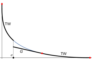
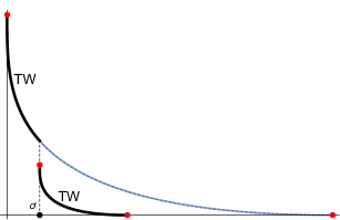
(c)	(d)

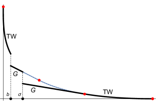
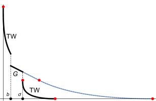
Figure 3. Examples of traffic jams obtained by inserting a roadblock at $\sigma$ (a,c) or a slowdown on $(\sigma,+\infty)$ (b,d). There is an additional roadblock at $b$ in pictures (c,d) generating a Gaussian phase before the jam at $\sigma$. The speed function ${\boldsymbol{\upxi}}(x)$ in all examples is piecewise constant. Dashed and solid curves are limit shapes before and after creating a traffic jam at $\sigma$, respectively. Tracy–Widom and Gaussian phases related to solid curves are also indicated. Solid red dots stand for points where a curved shape is tangent to a straight line.

While computer experiments suggest that the fluctuations on both sides of a traffic jam (of any of the two above types) are uncorrelated, the microscopic behavior of particles is expected to be very different depending on the type of the jam. Namely, if a jam at $\sigma$ is caused by a roadblock then there should be one very large stack of particles located precisely at $\sigma$. On the other hand, if a jam is caused by a slowdown then the buildup of particles should happen to the right of $\sigma$ (but very close to it), and locations of large stacks of particles there will be random. A more detailed study of the behavior of the model close to a traffic jam will be performed in a future publication.

2.6. Pre-limit Fredholm determinant

The starting point of our asymptotic analysis is the following Fredholm determinantal formula for the $q$-Laplace transform of the height function $\mathfrak{h}_{\mathbf{X}(t)}$ of the exponential jump model (before the ${\uplambda}\to+\infty$ limit):

Theorem 2.14.

Fix $t>0$ and $x\in\mathbb{R}_{>0}$. We have for any $\zeta\in\mathbb{C}\setminus\mathbb{R}_{\geq 0}$:

$$\mathop{\mathbb{E}}\frac{1}{\bigl{(}\zeta q^{\mathfrak{h}_{\mathbf{X}(t)}(x)};q\bigr{)}_{\infty}}=\det\bigl{(}1+K_{\zeta}\bigr{)}_{L^{2}(C_{a,\varphi})},$$ (2.14)

where the contour $C_{a,\varphi}$ is given in Definition 3.6 below with $0<a<\mathcal{W}_{x}$ and $\varphi\in(0,\pi/2)$. The kernel $K_{\zeta}$ in (2.14) is

$$K_{\zeta}(w,w^{\prime}):=\frac{1}{2\pi\mathbf{i}}\int_{D_{w}}\Gamma(-\mathsf{u})\Gamma(1+\mathsf{u})(-\zeta)^{\mathsf{u}}\frac{g(w)}{g(q^{\mathsf{u}}w)}\frac{d\mathsf{u}}{q^{\mathsf{u}}w-w^{\prime}},\qquad w,w^{\prime}\in C_{a,\varphi},$$ (2.15)

with the contour $D_{w}$ as in Definition 3.10 below, and

$$g(w):=\frac{1}{(w/{\boldsymbol{\upxi}}(0);q)_{\infty}}\prod_{b\in\mathbf{B},\,b<x}\frac{(w\mathbf{p}(b)/{\boldsymbol{\upxi}}(b);q)_{\infty}}{(w/{\boldsymbol{\upxi}}(b);q)_{\infty}}\exp\biggl{\{}-tw+{\uplambda}\int_{0}^{x}\phi_{0}\biggl{(}\frac{w}{{\boldsymbol{\upxi}}(y)}\biggr{)}dy\biggr{\}}.$$ (2.16)

We prove Theorem 2.14 in Section 3. The asymptotic analysis of the Fredholm determinantal formula (2.14) performed in Section 4 leads to our main result, Theorem 2.12.

3. From a vertex model to the exponential model

In this section we explain how the inhomogeneous exponential jump model defined in Section 2.1 arises as a degeneration of the stochastic higher spin six vertex model studied in [Bor17], [CP16], [BP16]. We also employ the $q$-moment formulas obtained in the latter paper to prove our main pre-limit Fredholm determinantal formula (Theorem 2.14).

3.1. Stochastic higher spin six vertex model

For future convenience we describe the stochastic higher spin six vertex model in the language of particle systems. Moreover, to avoid unnecessary parameters and limit transitions we only focus on the time-homogeneous model with the step Bernoulli boundary condition (about the name see Section 3.2 below). This model is a discrete time Markov chain $\{\mathbf{{X}}_{\mathrm{v}}(\mathfrak{t})\}_{\mathfrak{t}=0,1,\ldots}$ on the space of finite particle configurations $\mathrm{Conf}_{\bullet}(\mathbb{Z}_{\geq 1})$ depending on the parameters

$$q\in(0,1);\qquad u\in(0,+\infty);\qquad{\boldsymbol{\upxi}}(0)\in(0,+\infty);\qquad\upxi_{i}\in(0,+\infty),\quad\mathsf{s}_{i}\in(-1,0),\quad i\in\mathbb{Z}_{\geq 1},$$ (3.1)

such that $\upxi_{i}$ and $\mathsf{s}_{i}$ are uniformly bounded away from the endpoints of their corresponding intervals. The parameter ${\boldsymbol{\upxi}}(0)$ will eventually become the rate at which new particles are added in the inhomogeneous exponential jump model, so we can already use this notation here.

Definition 3.1 (Stochastic higher spin six vertex model).

Under $\mathbf{{X}}_{\mathrm{v}}(\mathfrak{t})$ during each step of the discrete time, the particle configuration $\eta=(\eta(1),\eta(2),\ldots)$ (where $\eta(i)\geq 0$ is the number of particles at location $i\in\mathbb{Z}_{\geq 1}$) is randomly updated to

$$\eta^{\prime}=(\eta^{\prime}(1),\eta^{\prime}(2),\eta^{\prime}(3),\ldots)=\left(\eta(1)-h(1)+h(0),\eta(2)-h(2)+h(1),\eta(3)-h(3)+h(2),\ldots\right),$$

where $h(0)\in\left\{0,1\right\}$ is the number of new particles entering the system, and $h(i)\in\left\{0,1\right\}$, $i\geq 1$, is the number of particles which moved from location $i$ to location $i+1$ during this time step (so particles move only to the right). The update propagates from left to right and is governed by the following probabilities (where $i=1,2,\ldots$):

$$\mathbb{P}\left(h(0)=k\right) =\frac{{\boldsymbol{\upxi}}(0)u}{1+{\boldsymbol{\upxi}}(0)u}\mathbf{1}_{k=1}+\frac{1}{1+{\boldsymbol{\upxi}}(0)u}\mathbf{1}_{k=0};$$ (3.2)

$$\mathbb{P}\left(h(i)=k\mid h(i-1)=0\right) =\frac{-\upxi_{i}\mathsf{s}_{i}u(1-q^{\eta(i)})}{1-\upxi_{i}\mathsf{s}_{i}u}\mathbf{1}_{k=1}+\frac{1-\upxi_{i}\mathsf{s}_{i}uq^{\eta(i)}}{1-\upxi_{i}\mathsf{s}_{i}u}\mathbf{1}_{k=0};$$ (3.3)

$$\mathbb{P}\left(h(i)=k\mid h(i-1)=1\right) =\frac{\mathsf{s}_{i}^{2}q^{\eta(i)}-\upxi_{i}\mathsf{s}_{i}u}{1-\upxi_{i}\mathsf{s}_{i}u}\mathbf{1}_{k=1}+\frac{1-\mathsf{s}_{i}^{2}q^{\eta(i)}}{1-\upxi_{i}\mathsf{s}_{i}u}\mathbf{1}_{k=0}.$$ (3.4)

Because the configurations are finite and all weights in (3.3)–(3.4) are uniformly bounded away from $0$ and $1$, almost surely there exists $M$ such that $h(j)=0$ for all $j>M$, which means that the random update $\eta\mapsto\eta^{\prime}$ eventually stops. See Figure 4.

probabilities	$\dfrac{1-\upxi_{i}\mathsf{s}_{i}uq^{\eta(i)}}{1-\upxi_{i}\mathsf{s}_{i}u}\rule{0.0pt}{22.0pt}$	$\dfrac{-\upxi_{i}\mathsf{s}_{i}u(1-q^{\eta(i)})}{1-\upxi_{i}\mathsf{s}_{i}u}$	$\dfrac{\mathsf{s}^{2}_{i}q^{\eta(i)}-\upxi_{i}\mathsf{s}_{i}u}{1-\upxi_{i}\mathsf{s}_{i}u}$	$\dfrac{1-\mathsf{s}^{2}_{i}q^{\eta(i)}}{1-\upxi_{i}\mathsf{s}_{i}u}$ —
moves in $\mathbf{{X}}_{\mathrm{v}}(\mathfrak{t})$
vertex configurations

Figure 4. Probabilities (3.3)–(3.4) of individual moves in the particle system $\mathbf{{X}}_{\mathrm{v}}(\mathfrak{t})$ and their interpretation in terms of vertex weights: vertical arrows correspond to particles and horizontal arrows — to their moves during one step of the discrete time.

Probabilities (3.3)–(3.4) have a very special property which justifies their definition: they satisfy (a version of) the Yang–Baxter equation. We do not reproduce it here and refer to [Man14], [Bor17], [CP16], [BP16a], [BP16] for details in the context of $U_{q}(\widehat{\mathfrak{sl}_{2}})$ vertex models, and to [Bax07] for a general background. The Yang–Baxter equation is a key tool used in [BP16] to compute averages of certain observables of the higher spin six vertex model in a contour integral form which we recall in Section 3.5 below.

Setting $\mathsf{s}_{i}^{2}\equiv 1/q$ turns $\mathbf{{X}}_{\mathrm{v}}(\mathfrak{t})$ into the stochastic six vertex model in which at most one particle per location $i\in\mathbb{Z}_{\geq 1}$ is allowed. If a new particle from $i-1$ decides to move on top of a particle already present at $i$, then the particle at $i$ gets displaced to the right (i.e., if $\eta(i)=1$ and $h(i-1)=1$, then $h(i)=1$ with probability $1$). This model was introduced in [GS92], and its asymptotic behavior was investigated in [BCG16], [AB16], [Agg16], [Bor16].

3.2. Remark. Boundary conditions

The step Bernoulli boundary condition for $\mathbf{{X}}_{\mathrm{v}}(\mathfrak{t})$ corresponds to particles entering the system at location $1$ independently at each time step with probability ${\boldsymbol{\upxi}}(0)u/(1+{\boldsymbol{\upxi}}(0)u)$, see (3.2). The term follows [AB16] where this type of boundary condition for the stochastic six vertex model was connected with the step Bernoulli (also sometimes called half stationary) initial configuration for the ASEP [TW09a]. Formulas for the $q$-moments are also available for the step boundary condition corresponding to $\mathbb{P}\left(h(0)=1\right)=1$ in (3.2) (i.e., a new particle enters at location $1$ at every time step), see [BP16] or [OP16].

The step boundary condition on $\mathbb{Z}_{\geq 1}$ can be degenerated to the step Bernoulli one on $\mathbb{Z}_{\geq 2}$ in two ways (related via the fusion procedure [KRS81], [CP16]). One way involves sending $\mathsf{s}_{1}\to 0$ and $\upxi_{1}\to+\infty$ such that $\alpha=-\upxi_{1}\mathsf{s}_{1}>0$ is fixed. In this limit we get the system with the step Bernoulli boundary condition on $\mathbb{Z}_{\geq 2}$, in which the role of ${\boldsymbol{\upxi}}(0)$ is played by $\alpha$.

Another way [BP16, Section 6.6] deals with time-homogeneous parameters $u_{1},u_{2},\ldots$ (with $u_{\mathfrak{t+1}}$ used during time step $\mathfrak{t}\to\mathfrak{t}+1$). Specializing the first $K$ of them into a geometric progression, formally putting $\upxi_{1}=\mathsf{s}_{1}$, and sending $K\to+\infty$ places infinitely many particles at location $1$. Probabilities (3.3)–(3.4) with $\eta(1)=+\infty$ reduce to (3.2) with the role of ${\boldsymbol{\upxi}}(0)$ played by $-\mathsf{s}_{1}^{2}$ (which is assumed positive), and this also leads to a system with the step Bernoulli boundary condition on $\mathbb{Z}_{\geq 2}$.

This second way suggests that in the process $\mathbf{{X}}_{\mathrm{v}}(\mathfrak{t})$ on $\mathbb{Z}_{\geq 1}$ described in Section 3.1 one can for convenience put an infinite stack of particles at location $0$, similarly to the exponential model (see Section 2.1).

3.3. Half-continuous vertex model

Let us take the limit as $u\searrow 0$ and $\mathfrak{t}\to+\infty$ so that $u\mathfrak{t}\to t\in\mathbb{R}_{\geq 0}$. Here $t$ is the rescaled continuous time. The expansions as $u\searrow 0$ of probabilities (3.2)–(3.4) are

$$\mathbb{P}\left(h(0)=k\right) =\left({\boldsymbol{\upxi}}(0)u+O(u^{2})\right)\mathbf{1}_{k=1}+\left(1+O(u)\right)\mathbf{1}_{k=0};$$ (3.5)

$$\mathbb{P}\left(h(i)=k\mid h(i-1)=0\right) =\left(-\upxi_{i}\mathsf{s}_{i}u(1-q^{\eta(i)})+O(u^{2})\right)\mathbf{1}_{k=1}+\left(1+O(u)\right)\mathbf{1}_{k=0};$$ (3.6)

$$\mathbb{P}\left(h(i)=k\mid h(i-1)=1\right) =\left(\mathsf{s}_{i}^{2}q^{\eta(i)}+O(u)\right)\mathbf{1}_{k=1}+\left(1-\mathsf{s}_{i}^{2}q^{\eta(i)}+O(u)\right)\mathbf{1}_{k=0}.$$ (3.7)

These expansions imply that the $u\searrow 0$ limit leads to the following system:

Definition 3.2 (Half-continuous vertex model).

The half-continuous stochastic higher spin six vertex model (or the half-continuous vertex model, for short) is a continuous time Markov process $\left\{\mathbf{X}_{\mathrm{hc}}(t)\right\}_{t\geq 0}$ on $\mathrm{Conf}_{\bullet}(\mathbb{Z}_{\geq 1})$ defined as follows. Initially all locations $i\in\mathbb{Z}_{\geq 1}$ are empty, and there is an infinite stack of particles at location $0$. Almost surely at most one particle can “wake up” and start moving in an instance of continuous time. Particles wake up by either leaving the infinite stack at $0$ at rate ${\boldsymbol{\upxi}}(0)$, or by leaving a stack of $\eta(i)$ particles at some location $i\in\mathbb{Z}_{\geq 1}$ at rate $\upxi_{i}(-\mathsf{s}_{i})(1-q^{\eta(i)})$. The wake up events at different locations are independent and have exponential waiting times.

Every particle which wakes up at some time moment $t\geq 0$ then instantaneously jumps to the right according to the following probability:

$$\mathbb{P}\bigl{(}\textnormal{the moving particle ends exactly at location $j>i$}\mid\textnormal{it started at $i\in\left\{0\right\}\cup\mathbb{Z}_{\geq 1}$}\bigr{)}\\ =\mathsf{s}_{i+1}^{2}\ldots\mathsf{s}_{j-1}^{2}q^{\eta_{\mathbf{X}_{\mathrm{hc}}(t)}(i+1)+\ldots+\eta_{\mathbf{X}_{\mathrm{hc}}(t)}(j-1)}\left(1-\mathsf{s}_{j}^{2}q^{\eta_{\mathbf{X}_{\mathrm{hc}}(t)}(j)}\right),$$ (3.8)

where $j>i$ is arbitrary and the quantities $\eta_{\mathbf{X}_{\mathrm{hc}}(t)}$ correspond to the configuration of particles before the moving particle started its jump. In words, to move past any location $k>i$ the moving particle flips a coin with probability of success $\mathsf{s}_{k}^{2}q^{\eta_{\mathbf{X}_{\mathrm{hc}}(t)}(k)}$. If the coin comes up a success, the particle continues to move, otherwise it stops at location $k$.

The process $\mathbf{X}_{\mathrm{hc}}(t)$ depends on $q$, ${\boldsymbol{\upxi}}(0)$, and the parameters $\upxi_{i}$, $\mathsf{s}_{i}$, where $i\geq 1$.

The fact that $\mathbf{X}_{\mathrm{hc}}(t)$ is a continuous time limit of $\mathbf{{X}}_{\mathrm{v}}(\mathfrak{t})$ follows by a standard application of a Poisson-type limit theorem, much like how a discrete time random walk on $\mathbb{Z}$ with jumps $\in\{0,1\}$ and with small probability of a jump by $1$ can be approximated in the continuous time limit by a Poisson jump process. Indeed, this is because up to any time $\mathfrak{t}=\lfloor tu^{-1}\rfloor$ the total number of particles in $\mathbf{{X}}_{\mathrm{v}}(\mathfrak{t})$ can be approximated by a Poisson random variable with parameter ${\boldsymbol{\upxi}}(0)t$, and conditioned on having a given number of particles the discrete time finite particle system is approximated by the corresponding continuous time finite particle system.

Remark 3.3.

A similar half-continuous limit of the stochastic six vertex model (the case $\mathsf{s}_{i}^{2}\equiv 1/q$) was considered recently in [BBW16], [Gho17], see also [BCG16].

3.4. Limit to continuous space

Consider the scaling limit of discrete to continuous space, $\mathbb{Z}_{\geq 1}\ni i\mapsto i\varepsilon\in\mathbb{R}_{>0}$ as $\varepsilon\searrow 0$. Let us show that under this limit the process $\mathbf{X}_{\mathrm{hc}}(t)$ becomes the inhomogeneous exponential jump model $\mathbf{X}(t)$ described in Section 2.1. Let us first describe the scaling of parameters of $\mathbf{X}_{\mathrm{hc}}(t)$ assuming that the parameters ${\uplambda}$, ${\boldsymbol{\upxi}}(x)$, $\mathbf{B}$, and $\mathbf{p}(b)$, $b\in\mathbf{B}$, of $\mathbf{X}(t)$ are given. Denote

$$\mathbf{B}^{\varepsilon}:=\left\{\lfloor\varepsilon^{-1}b\rfloor\colon b\in\mathbf{B}\right\}\subset\mathbb{Z}_{\geq 1},$$ (3.9)

and put

$$\begin{array}[]{lll}\mathsf{s}_{i}^{2}=e^{-\varepsilon{\uplambda}},&\qquad-\upxi_{i}\mathsf{s}_{i}={\boldsymbol{\upxi}}(i\varepsilon),&\qquad\textnormal{for}\quad i\in\mathbb{Z}_{\geq 1}\setminus\mathbf{B}^{\varepsilon};\\[3.0pt] \mathsf{s}_{i}^{2}=\mathbf{p}(b),&\qquad-\upxi_{i}\mathsf{s}_{i}={\boldsymbol{\upxi}}(b),&\qquad\textnormal{for}\quad i=\lfloor\varepsilon^{-1}b\rfloor\in\mathbf{B}^{\varepsilon}.\end{array}$$ (3.10)

Denote this $\varepsilon$-dependent process by $\mathbf{X}_{\mathrm{hc}}^{\varepsilon}(t)$. Because the rates at which new particles are added to both $\mathbf{X}_{\mathrm{hc}}^{\varepsilon}(t)$ and $\mathbf{X}(t)$ are the same, we can couple these processes so that they have the same Poisson number of particles at each time $t\geq 0$. This reduces the question of convergence of $\{\mathbf{X}_{\mathrm{hc}}^{\varepsilon}(t)\}_{t\geq 0}$ to $\{\mathbf{X}(t)\}_{t\geq 0}$ to finite particle systems. Because ${\boldsymbol{\upxi}}(x)$ is piecewise continuous with left and right limits, the rates at which particles decide to start moving in $\mathbf{X}_{\mathrm{hc}}^{\varepsilon}$ are close to those in $\mathbf{X}$. To conclude the convergence of $\{\mathbf{X}_{\mathrm{hc}}^{\varepsilon}(t)\}_{t\geq 0}$ to $\{\mathbf{X}(t)\}_{t\geq 0}$ it remains to observe that the limit as $\varepsilon\searrow 0$ of traveling probabilities (3.8) gives rise to (2.3), which is straightforward.

Let us summarize the development of Sections 3.1, 3.2, 3.3 and 3.4:

Proposition 3.4.

Under the sequence of limit transitions

$$\big{\{}\mathbf{{X}}_{\mathrm{v}}(\mathfrak{t})\big{\}}_{\mathfrak{t}=0,1,\ldots}\xrightarrow[\parbox{82.38885pt}{speed up time as $\mathfrak{t}=\lfloor tu^{-1}\rfloor$, $u\searrow 0$}]{}\big{\{}\mathbf{X}_{\mathrm{hc}}(t)\big{\}}_{t\geq 0}\xrightarrow[\parbox{147.4292pt}{rescale parameters $\upxi_{i}$, $\mathsf{s}_{i}$, $i\geq 1$, as in \eqref{scale_discrete_to_continuous_space1}--\eqref{scale_discrete_to_continuous_space2}, and rescale the space $\mathbb{Z}_{\geq 1}$ to $\mathbb{R}_{>0}$ }]{}\big{\{}\mathbf{X}(t)\big{\}}_{t\geq 0}$$

the stochastic higher spin six vertex model with the step Bernoulli boundary condition described in Section 3.1 converges to the inhomogeneous exponential jump model defined in Section 2.1.

3.5. $q$-moments for the half-continuous model

Here and in Sections 3.6, 3.7 and 3.8 below we prove Theorem 2.14. Except passing to the continuous space in the last step, the proof is quite similar to the treatment of $q$-moments and $q$-Laplace transforms performed in [BCF14], [FV15], [Bar15]. However, to make the present paper self-contained we discuss all the necessary steps, which are as follows:

1. First, in this subsection we recall a nested contour integral formula for the $q$-moments of the height function of the stochastic higher spin six vertex model, and take a (straightforward) limit to the $q$-moments in the half-continuous model.

2. In Section 3.6 we rewrite these $q$-moments for the half-continuous model in terms of contour integrals over certain infinite contours (which will be convenient for asymptotic analysis in Section 4).

3. In Section 3.7 we turn the $q$-moment formulas for the half-continuous model into a Fredholm determinantal formula for this model. This requires some technical work to justify choices of integration contours which will be optimal for asymptotics.

4. Finally, in Section 3.8 we pass to the limit to the continuous space, and obtain a Fredholm determinantal formula for the $q$-Laplace transform of the height function in the inhomogeneous exponential jump model.

Let the height function $\mathfrak{h}_{\mathbf{X}_{\mathrm{hc}}(t)}(k)$, $k\in\mathbb{Z}_{\geq 0}$, of the process on the discrete space be defined similarly to (2.1). We have $\mathfrak{h}_{\mathbf{X}_{\mathrm{hc}}(t)}(0)=+\infty$, and $\mathfrak{h}_{\mathbf{X}_{\mathrm{hc}}(t)}(M)=0$ for $M$ large enough. The next proposition is our first step towards Theorem 2.14.

Figure 5. A possible choice of nested integration contours in (3.12) for $\ell=3$. The contours $qw_{3}$ and $q^{2}w_{3}$ are shown dotted.

Proposition 3.5.

Assume that the parameters of the half-continuous model $\mathbf{X}_{\mathrm{hc}}(t)$ satisfy

$$\min\left({\boldsymbol{\upxi}}(0),\inf_{j\geq 1}\left\{-\upxi_{j}\mathsf{s}_{j}\right\}\right)>q\cdot\min\left({\boldsymbol{\upxi}}(0),\sup_{j\geq 1}\left\{-\upxi_{j}\mathsf{s}_{j}\right\}\right).$$ (3.11)

Then the $q$-moments of the height function of $\mathbf{X}_{\mathrm{hc}}(t)$ at any $k\in\mathbb{Z}_{\geq 1}$ are given by

$$\mathop{\mathbb{E}}q^{\ell\mathfrak{h}_{\mathbf{X}_{\mathrm{hc}}(t)}(k)}=(-1)^{\ell}q^{\frac{\ell(\ell-1)}{2}}\oint\frac{dw_{1}}{2\pi\mathbf{i}}\ldots\oint\frac{dw_{\ell}}{2\pi\mathbf{i}}\prod_{1\leq A<B\leq\ell}\frac{w_{A}-w_{B}}{w_{A}-qw_{B}}\\ \times\prod_{i=1}^{\ell}\left(\frac{e^{(q-1)tw_{i}}}{w_{i}(1-w_{i}/{\boldsymbol{\upxi}}(0))}\prod_{j=1}^{k-1}\frac{\upxi_{j}\mathsf{s}_{j}+\mathsf{s}_{j}^{2}w_{i}}{\upxi_{j}\mathsf{s}_{j}+w_{i}}\right),$$ (3.12)

where $\ell=1,2,\ldots$, the integration contours are positively oriented simple closed curves which encircle the poles ${\boldsymbol{\upxi}}(0)$ and $-\upxi_{j}\mathsf{s}_{j}$, $j=1,2,\ldots$, but not $0$, and the contour for $w_{A}$ contains the contour for $qw_{B}$ for all $A<B$ (see Figure 5).

Proof.

We start with the formula of [BP16, Corollary 10.3] which gives $q$-moments of the height function of the discrete time stochastic higher spin six vertex model with the step Bernoulli boundary condition on $\mathbb{Z}_{\geq 2}$. However, since our process $\mathbf{{X}}_{\mathrm{v}}(\mathfrak{t})$ lives on $\mathbb{Z}_{\geq 1}$, we need to shift the parameters by $1$. Thus, the formula yields for any $\ell\geq 1$ and $k\geq 0$:

$$\mathop{\mathbb{E}}q^{\ell\mathfrak{h}_{\mathbf{{X}}_{\mathrm{v}}(\mathfrak{t})}(k)}=(-1)^{\ell}q^{\frac{\ell(\ell-1)}{2}}\oint\frac{dw_{1}}{2\pi\mathbf{i}}\ldots\oint\frac{dw_{\ell}}{2\pi\mathbf{i}}\prod_{1\leq A<B\leq\ell}\frac{w_{A}-w_{B}}{w_{A}-qw_{B}}\\ \times\prod_{i=1}^{\ell}\left(\frac{1}{w_{i}(1-w_{i})}\prod_{j=0}^{k-1}\frac{\upxi_{j}-\mathsf{s}_{j}w_{i}}{\upxi_{j}-\mathsf{s}_{j}^{-1}w_{i}}\left(\frac{1-quw_{i}}{1-uw_{i}}\right)^{\mathfrak{t}}\right),$$ (3.13)

where $\upxi_{0}\equiv\mathsf{s}_{0}$ (and $-\mathsf{s}_{0}^{2}={\boldsymbol{\upxi}}(0)>0$), the integration contours are positively oriented and closed, encircle $\left\{\upxi_{i}\mathsf{s}_{i}\right\}_{i=0,1,\ldots}$, leave outside $0$, $1$ and $u^{-1}$, and the contour for $w_{A}$ contains the contour for $qw_{B}$ for all $A<B$. These contours exist thanks to (3.11). Formula (3.13) is obtained from a $q$-moment formula for the step boundary condition [BP16, Theorem 9.8] via the second of the limit transitions mentioned in Section 3.2.

Let us now assume that $k\geq 1$ since the case $k=0$ will not be needed for our asymptotic analysis. When $k\geq 1$ we get the following cancellation:

$$\frac{1}{1-w}\frac{\upxi_{0}-\mathsf{s}_{0}w}{\upxi_{0}-\mathsf{s}_{0}^{-1}w}=\frac{\mathsf{s}_{0}^{2}}{\mathsf{s}_{0}^{2}-w}=\frac{1}{1+w/{\boldsymbol{\upxi}}(0)}.$$

Let us change the variables as $w_{i}\to-w_{i}$. Then (3.13) turns into

$$\mathop{\mathbb{E}}q^{\ell\mathfrak{h}_{\mathbf{{X}}_{\mathrm{v}}(\mathfrak{t})}(k)}=(-1)^{\ell}q^{\frac{\ell(\ell-1)}{2}}\oint\frac{dw_{1}}{2\pi\mathbf{i}}\ldots\oint\frac{dw_{\ell}}{2\pi\mathbf{i}}\prod_{1\leq A<B\leq\ell}\frac{w_{A}-w_{B}}{w_{A}-qw_{B}}\\ \times\prod_{i=1}^{\ell}\left(\frac{1}{w_{i}(1-w_{i}/{\boldsymbol{\upxi}}(0))}\prod_{j=1}^{k-1}\frac{\upxi_{j}\mathsf{s}_{j}+\mathsf{s}_{j}^{2}w_{i}}{\upxi_{j}\mathsf{s}_{j}+w_{i}}\left(\frac{1+quw_{i}}{1+uw_{i}}\right)^{\mathfrak{t}}\right),$$

with the integration contours as in Figure 5. Putting $\mathfrak{t}=\lfloor tu^{-1}\rfloor$ and taking $u\searrow 0$ (note that this is allowed by the integration contours) leads to the desired formula for the $q$-moments of the height function of the half-continuous model $\mathbf{X}_{\mathrm{hc}}(t)$. ∎

3.6. Rewriting $q$-moment formulas

Let us introduce new integration contours:

Definition 3.6.

Let $C_{a,\varphi}$, $a\in(0,+\infty)$, $\varphi\in(0,\pi/2)$, be the contour including two rays at the angles $\pm\varphi$ with the real line which meet at the point $a$, and such that the imaginary part decreases along this contour. Namely,

$$C_{a,\varphi}:=\big{\{}a-\mathbf{i}ye^{\mathbf{i}\varphi\mathop{\mathrm{sgn}}(y)}\colon y\in\mathbb{R}\big{\}}.$$ (3.14)

See Figure 6 for an illustration.

Figure 6. A possible choice of contours $C_{a_{i},\varphi}$, $i=1,2,3$, in Proposition 3.7 for $\ell=3$. The contours $qC_{a_{3},\varphi}$ and $q^{2}C_{a_{3},\varphi}$ are shown dotted. The contour

Proposition 3.7.

If the parameters of the half-continuous vertex model satisfy (3.11), then the $q$-moments $\mathop{\mathbb{E}}q^{\ell\mathfrak{h}_{\mathbf{X}_{\mathrm{hc}}(t)}(k)}$, $k,\ell\geq 1$, $t>0$, are given by the same formula as in the right-hand side of (3.12), but with $w_{j}$ integrated over $C_{a_{j},\varphi}$, where $\varphi\in(0,\pi/2)$ and $a_{1},\ldots,a_{\ell}$ are such that

$$0<a_{j}<qa_{j+1},\quad j=1,\ldots,\ell-1;\qquad a_{\ell}<\min\left({\boldsymbol{\upxi}}(0),\inf_{j\geq 1}\left\{-\upxi_{j}\mathsf{s}_{j}\right\}\right).$$

Proof.

This statement is established in the same way as [BCF14, Lemma 4.10], by expanding the closed contours for $w_{1},\ldots,w_{\ell}$ in (3.12) one by one to the right, and using the fact that the exponent $e^{(q-1)t\sum_{i}w_{i}}$ in the integrand makes the integrals over the far right parts of the contours negligible. ∎

Proposition 3.8.

The $q$-moments $\mathop{\mathbb{E}}q^{\ell\mathfrak{h}_{\mathbf{X}_{\mathrm{hc}}(t)}(k)}$, $k,\ell\geq 1$, $t>0$, of the half-continuous vertex model can be rewritten in the following form with all integrals over one and the same contour $C_{a,\varphi}$ with $\varphi\in(0,\pi/2)$ and $0<a<\min\bigl{(}{\boldsymbol{\upxi}}(0),\inf_{j\geq 1}\left\{-\upxi_{j}\mathsf{s}_{j}\right\}\bigr{)}$:

$$\mathop{\mathbb{E}}q^{\ell\mathfrak{h}_{\mathbf{X}_{\mathrm{hc}}(t)}(k)}=(q;q)_{\ell}\sum_{\begin{subarray}{c}\mu\vdash\ell\\ \mu=1^{m_{1}}2^{m_{2}}\ldots\end{subarray}}\frac{1}{m_{1}!m_{2}!\cdots}\frac{1}{(2\pi\mathbf{i})^{l(\mu)}}\int\ldots\int\mathop{\mathrm{det}}\limits_{i,j=1}^{l(\mu)}\left[\frac{1}{w_{i}q^{\mu_{i}}-w_{j}}\right]\\ \times\prod_{j=1}^{l(\mu)}f^{\mathrm{hc}}(w_{j})f^{\mathrm{hc}}(qw_{j})\ldots f^{\mathrm{hc}}(q^{\mu_{j}-1}w_{j})dw_{j},$$ (3.15)

where the sum is over all partitions $\mu$ of $\ell$ (i.e., $\ell=\sum_{i}\mu_{i}$) having $m_{1}$ parts equal to $1$, $m_{2}$ parts equal to $2$, etc., $l(\mu)$ denotes the number of nonzero parts in $\mu$, and

$$f^{\mathrm{hc}}(w):=\frac{e^{(q-1)tw}}{1-w/{\boldsymbol{\upxi}}(0)}\prod_{j=1}^{k-1}\frac{\upxi_{j}\mathsf{s}_{j}+\mathsf{s}_{j}^{2}w}{\upxi_{j}\mathsf{s}_{j}+w}.$$ (3.16)

Proof.

This is [BC14, Proposition 3.2.1] or [BCPS15, Proposition 7.4]. ∎

The $q$-moment formula in Proposition 3.8 implies that we can drop condition (3.11) on the parameters ${\boldsymbol{\upxi}}(0)$, $\upxi_{j},\mathsf{s}_{j}$, $j\geq 1$ (which was present in contour integral formulas with bounded contours coming from [BP16]). From now on we only assume that ${\boldsymbol{\upxi}}(0)>0$, $\upxi_{j}>0$ are uniformly bounded away from $0$ and $+\infty$, and $\mathsf{s}_{j}\in(-1,0)$ are uniformly bounded away from $-1$ and $0$, and with these assumptions the $q$-moment formula (3.15) continues to hold.

3.7. Fredholm determinantal formulas for the half-continuous model

Our first Fredholm determinantal formula follows by taking a generating function of the $q$-moments given in Proposition 3.8:

Proposition 3.9.

Fix $t>0$ and $k\in\mathbb{Z}_{\geq 1}$. For any $0<a<\min\bigl{(}{\boldsymbol{\upxi}}(0),\inf_{j\geq 1}\left\{-\upxi_{j}\mathsf{s}_{j}\right\}\bigr{)}$, $\varphi\in(0,\pi/2)$, and $\zeta\in\mathbb{C}$ with sufficiently small $|\zeta|$ we have

$$\mathop{\mathbb{E}}\frac{1}{\bigl{(}\zeta q^{\mathfrak{h}_{\mathbf{X}_{\mathrm{hc}}(t)}(k)};q\bigr{)}_{\infty}}=\det\bigl{(}1+K_{\zeta}^{(1),\mathrm{hc}}\bigr{)}_{L^{2}(\mathbb{Z}_{>0}\times C_{a,\varphi})},$$ (3.17)

where the kernel $K_{\zeta}^{(1),\mathrm{hc}}$ is given by

$$K_{\zeta}^{(1),\mathrm{hc}}(n_{1},w_{1};n_{2},w_{2})=\frac{\zeta^{n_{1}}f^{\mathrm{hc}}(w_{1})f^{\mathrm{hc}}(qw_{1})\cdots f^{\mathrm{hc}}(q^{n_{1}-1}w_{1})}{q^{n_{1}}w_{1}-w_{2}},$$ (3.18)

with $f^{\mathrm{hc}}(w)$ defined in (3.16).

The Fredholm determinant of a kernel on $\mathbb{Z}_{>0}\times C_{a,\varphi}$ is defined similarly to (2.12), but along with integrating determinants of $K_{\zeta}^{(1),\mathrm{hc}}$ of sizes $M=1,2,\ldots$ in the continuous variables $w_{1},\ldots,w_{M}\in C_{a,\varphi}$ we also sum them over the discrete variables $n_{1},\ldots,n_{M}\in\mathbb{Z}_{>0}$. See also (3.26) below.

Proof.

We first use the $q$-binomial theorem [GR04, (1.3.2)] to write

$$\mathop{\mathbb{E}}\frac{1}{(\zeta q^{\mathfrak{h}_{\mathbf{X}_{\mathrm{hc}}(t)}(k)};q)_{\infty}}=\sum_{\ell=0}^{\infty}\frac{\zeta^{\ell}\mathop{\mathbb{E}}q^{\ell\mathfrak{h}_{\mathbf{X}_{\mathrm{hc}}(t)}(k)}}{(q;q)_{\ell}}.$$

Because $q^{\ell\mathfrak{h}_{\mathbf{X}_{\mathrm{hc}}(t)}(k)}\leq 1$, the series converges for small enough $|\zeta|$, which justifies the interchange of the summation and the expectation. Using the formula of Proposition 3.8 for $\mathop{\mathbb{E}}q^{\ell\mathfrak{h}_{\mathbf{X}_{\mathrm{hc}}(t)}(k)}$ we can reorganize the above summation (see [BC14, Proposition 3.2.8] for details) and write

$$\mathop{\mathbb{E}}\frac{1}{(\zeta q^{\mathfrak{h}_{\mathbf{X}_{\mathrm{hc}}(t)}(k)};q)_{\infty}}=\sum_{M=0}^{\infty}\frac{1}{M!}\sum_{n_{1},\ldots,n_{M}\in\mathbb{Z}_{>0}}\int_{C_{a,\varphi}}\ldots\int_{C_{a,\varphi}}\mathop{\mathrm{det}}\limits_{i,j=1}^{M}\left[\frac{1}{q^{n_{i}}w_{i}-w_{j}}\right]\\ \times\prod_{j=1}^{M}\zeta^{n_{j}}f^{\mathrm{hc}}(w_{j})f^{\mathrm{hc}}(qw_{j})\ldots f^{\mathrm{hc}}(q^{n_{j}-1}w_{j})\frac{dw_{j}}{2\pi\mathbf{i}}.$$ (3.19)

This coincides with the Fredholm expansion of $\det\bigl{(}1+K_{\zeta}^{(1),\mathrm{hc}}\bigr{)}_{L^{2}(\mathbb{Z}_{>0}\times C_{a,\varphi})}$ in the right-hand side of (3.17) with the kernel given by (3.18). To finish the proof and show that identity (3.17) holds numerically for small $|\zeta|$, we need to justify that the expansion in (3.19) converges absolutely. First, observe that $f^{\mathrm{hc}}(q^{n}w)$ given by (3.16) is bounded on the contour $C_{a,\varphi}$ uniformly in $n\geq 0$, and $f^{\mathrm{hc}}(w)$ decays exponentially as $|w|$ grows. This implies that

$$|f^{\mathrm{hc}}(w_{j})f^{\mathrm{hc}}(qw_{j})\ldots f^{\mathrm{hc}}(q^{n_{j}-1}w_{j})|\leq B_{1}^{n_{j}}e^{-c\mathop{\mathrm{Re}}(w_{j})}.$$ (3.20)

Next, observe that $\min_{w_{1},w_{2}\in C_{a,\varphi}}|q^{n}w_{1}-w_{2}|=(1-q^{n})a\sin\varphi\geq(1-q)a\sin\varphi$ for any $n\in\mathbb{Z}_{>0}$, and so by the Hadamard’s inequality we have

$$\left|\mathop{\mathrm{det}}\limits_{i,j=1}^{M}\left[\frac{1}{q^{n_{i}}w_{i}-w_{j}}\right]\right|\leq B_{2}^{M}M^{M/2}.$$

Therefore, the sum of integrals of the absolute values in the right-hand side of (3.19) can be estimated as

$$\sum_{M\geq 0}\frac{B_{2}^{M}M^{M/2}}{M!}\left(\sum_{n\geq 1}B_{1}^{n}\zeta^{n}B_{3}\right)^{M},$$

where $B_{3}$ arises from integrating the exponent in (3.20). The inside geometric series in $n$ converges for sufficiently small $|\zeta|$, and the series in $M$ converges thanks to the factorial in the denominator. This completes the proof. ∎

Following [BCF14], let us define another contour which will play a role in the next Fredholm determinantal formula.

Definition 3.10.

For $R,d>0$ let

$$D_{R,d}:=\bigl{(}R-\mathbf{i}\infty,R-\mathbf{i}d\bigr{]}\cup\bigl{(}R-\mathbf{i}d,\tfrac{1}{2}-\mathbf{i}d\bigr{]}\cup\bigl{(}\tfrac{1}{2}-\mathbf{i}d,\tfrac{1}{2}+\mathbf{i}d\bigr{]}\cup\bigl{(}\tfrac{1}{2}+\mathbf{i}d,R+\mathbf{i}d\bigr{]}\cup\bigl{(}R+\mathbf{i}d,R+\mathbf{i}\infty\bigr{)},$$ (3.21)

oriented so that the imaginary part does not decrease along $D_{R,d}$. Now, for every $w\in C_{a,\varphi}$, where $a>0$, $\varphi\in(0,\pi/2)$, let us choose $R(w),d(w)$ such that:

1. For any $\mathsf{u}\in D_{R(w),d(w)}$ we have $\arg(w(q^{\mathsf{u}}-1))\in(\pi/2+b,3\pi/2-b)$, where $b=\pi/4-\varphi/2$.

2. For any $\mathsf{u}\in D_{R(w),d(w)}$ the point $q^{\mathsf{u}}w$ stays to the left of the contour $C_{a,\varphi}$.

Denote the resulting contour $D_{R(w),d(w)}$ simply by $D_{w}$. By [BCF14, Remark 4.9], the contour $D_{w}$ exists, and for large $|w|$ it suffices to take $d(w)\sim B_{d}|w|^{-1}$ and $R(w)\sim B_{R}\log|w|$ for some constants $B_{d},B_{R}>0$. See Figure 7 for an illustration.

Figure 7. Left: the contour $D_{R,d}$. Right: the points $q^{\mathsf{u}}$ for $\mathsf{u}\in D_{R,d}$. The angle indicated in the picture should be less than $b=\pi/4-\varphi/2$ in order to satisfy the condition $\arg(w(q^{\mathsf{u}}-1))\in(\pi/2+b,3\pi/2-b)$.

Proposition 3.11.

Fix $t>0$ and $k\in\mathbb{Z}_{\geq 1}$. We have for any $\zeta\in\mathbb{C}\setminus\mathbb{R}_{\geq 0}$:

$$\mathop{\mathbb{E}}\frac{1}{\bigl{(}\zeta q^{\mathfrak{h}_{\mathbf{X}_{\mathrm{hc}}(t)}(k)};q\bigr{)}_{\infty}}=\det\bigl{(}1+K_{\zeta}^{(2),\mathrm{hc}}\bigr{)}_{L^{2}(C_{a,\varphi})},$$ (3.22)

where the contour $C_{a,\varphi}$ is given in Definition 3.6 with $0<a<\min\bigl{(}{\boldsymbol{\upxi}}(0),\inf_{j\geq 1}\left\{-\upxi_{j}\mathsf{s}_{j}\right\}\bigr{)}$ and $\varphi\in(0,\pi/2)$. The kernel in (3.22) is

$$K_{\zeta}^{(2),\mathrm{hc}}(w,w^{\prime})=\frac{1}{2\pi\mathbf{i}}\int_{D_{w}}\Gamma(-\mathsf{u})\Gamma(1+\mathsf{u})(-\zeta)^{\mathsf{u}}\frac{g^{\mathrm{hc}}(w)}{g^{\mathrm{hc}}(q^{\mathsf{u}}w)}\frac{d\mathsf{u}}{q^{\mathsf{u}}w-w^{\prime}},$$ (3.23)

with the contour $D_{w}$ as in Definition 3.10 and where $g^{\mathrm{hc}}(w)$ is expressed through $f^{\mathrm{hc}}(w)$ (3.16) via

$$g^{\mathrm{hc}}(w):=f^{\mathrm{hc}}(w)f^{\mathrm{hc}}(qw)\ldots=\frac{e^{-tw}}{(w/{\boldsymbol{\upxi}}(0);q)_{\infty}}\prod_{j=1}^{k-1}\frac{(-w\mathsf{s}_{j}\upxi_{j}^{-1};q)_{\infty}}{(-w\mathsf{s}_{j}^{-1}\upxi_{j}^{-1};q)_{\infty}}.$$ (3.24)

Proof.

Step 1. We first prove (3.22) for small $|\zeta|$ by rewriting the previous formula of Proposition 3.9, and then will analytically continue in $\zeta$ using the properties of the contour $C_{a,\varphi}$. To rewrite the sums coming from the $\mathbb{Z}_{>0}$ part of the Fredholm determinant in (3.17), we use the Mellin–Barnes summation formula (e.g., [BCF14, Lemma 7.1]) which follows from the fact that $\mathop{\mathrm{Res}}_{\mathsf{u}=n}\Gamma(-\mathsf{u})\Gamma(1+\mathsf{u})=(-1)^{n+1}$:

$$\sum_{n=1}^{\infty}F(q^{n})\zeta^{n}=\frac{1}{2\pi\mathbf{i}}\int_{C_{1,2,\ldots}}\Gamma(-\mathsf{u})\Gamma(1+\mathsf{u})(-\zeta)^{\mathsf{u}}F(q^{\mathsf{u}})d\mathsf{u},\qquad|\zeta|<1,\quad\zeta\notin\mathbb{R}_{\geq 0},$$ (3.25)

where the contour $C_{1,2,\ldots}$ encircles points $1,2,\ldots$ and winds around them in the negative direction, and encircles no other singularities of $F(q^{\mathsf{u}})$. For the above equality to hold, the series in the left-hand side must converge, and the integral in the right-hand side must be able to be approximated by integrals over a sequence of (negatively oriented) contours $C_{\mathsf{k}}$, $\mathsf{k}=1,2,\ldots$, such that:

1. Each contour $C_{\mathsf{k}}$ encircles $1,\ldots,\mathsf{k}$ and no other singularities of the integrand;

2. The contours $C_{\mathsf{k}}$ partly coincide with $C_{1,2,\ldots}$;

3. The integral over the symmetric difference of $C_{\mathsf{k}}$ and $C_{1,2,\ldots}$ goes to zero as $\mathsf{k}\to\infty$.

The Fredholm determinant in the right-hand side of (3.17) looks as

$$\det\bigl{(}1+K_{\zeta}^{(1),\mathrm{hc}}\bigr{)}_{L^{2}(\mathbb{Z}_{>0}\times C_{a,\varphi})}\\ =1+\sum_{M=1}^{\infty}\frac{1}{M!}\sum_{\sigma\in S(M)}(-1)^{\sigma}\prod_{j=1}^{M}\int_{C_{a,\varphi}}\frac{dw_{j}}{2\pi\mathbf{i}}\sum_{n_{j}=1}^{\infty}\frac{\zeta^{n_{j}}}{q^{n_{j}}w_{j}-w_{\sigma(j)}}\frac{g^{\mathrm{hc}}(w_{j})}{g^{\mathrm{hc}}(q^{n_{j}}w_{j})}.$$ (3.26)

We aim to apply (3.25) to each of the sums over $n_{j}$ above (which converge for sufficiently small $|\zeta|$, as follows from the proof of Proposition 3.9), that is, with

$$F(q^{\mathsf{u}})=F_{w,w^{\prime}}(q^{\mathsf{u}}):=\frac{g^{\mathrm{hc}}(w)}{(q^{\mathsf{u}}w-w^{\prime})g^{\mathrm{hc}}(q^{\mathsf{u}}w)},$$ (3.27)

where $w,w^{\prime}\in C_{a,\varphi}$ are fixed. For that we define $C_{\mathsf{k}}$ to be a closed contour which coincides with $D_{w}$ of Definition 3.10 inside the disc of radius $\mathsf{k}+\frac{1}{2}$ centered at $0$ and which is closed by an arc of the corresponding circle, see Figure 8. The contour $D_{w}$ will then serve as $C_{1,2,\ldots}$.

Figure 8. The contour $C_{\mathsf{k}}$ (solid) used in the proof of Proposition 3.11, and the parts $C_{\mathsf{k}}^{seg}$ and $C_{\mathsf{k}}^{arc}$ (dotted) of the symmetric difference between $C_{\mathsf{k}}$ and $D_{w}$.

Because of our definitions of $C_{a,\varphi}$ and $D_{w}$, the contours $C_{\mathsf{k}}$ and $D_{w}$ do not encircle any $\mathsf{u}$ singularities of the integrand $\Gamma(-\mathsf{u})\Gamma(1+\mathsf{u})(-\zeta)^{\mathsf{u}}F_{w,w^{\prime}}(q^{\mathsf{u}})$ except for the poles of $\Gamma(-\mathsf{u})$. Indeed, the part of the plane to the right of $D_{w}$ maps under $\mathsf{u}\mapsto q^{\mathsf{u}}$ to the union of the disc and the sector in Figure 7, right. Therefore, because $q^{\mathsf{u}}w$ lies to the left of $C_{a,\varphi}\ni w^{\prime}$, the denominator $q^{\mathsf{u}}w-w^{\prime}$ does not vanish for $\mathsf{u}$ to the right of $D_{w}$. Moreover, poles coming from $g^{\mathrm{hc}}(q^{\mathsf{u}}w)=0$ are $q^{\mathsf{u}}w=-\upxi_{j}\mathsf{s}_{j}^{-1}q^{-m}$, $m\in\mathbb{Z}_{\geq 0}$, and they also do not occur for $\mathsf{u}$ to the right of $D_{w}$ because $q^{\mathsf{u}}w$ is to the left of $C_{a,\varphi}$ while the points $-\upxi_{j}\mathsf{s}_{j}^{-1}q^{-m}$ are all to the right of $C_{a,\varphi}$.

Thus, to apply (3.25) to (3.26) it remains to show that the integrals over the symmetric difference of $D_{w}$ and $C_{\mathsf{k}}$ go to zero as $\mathsf{k}\to+\infty$. The symmetric difference contains two straight lines the union of which is denoted by $C_{\mathsf{k}}^{seg}$ and an arc denoted by $C_{\mathsf{k}}^{arc}$, see Figure 8. First, observe that for fixed $w,w^{\prime}\in C_{a,\varphi}$ the function $F_{w,w^{\prime}}(q^{\mathsf{u}})$ is uniformly bounded in $\mathsf{u}\in C_{\mathsf{k}}^{seg}\cup C_{\mathsf{k}}^{arc}$.

Consider $C_{\mathsf{k}}^{seg}$. We have $|(-\zeta)^{\mathsf{u}}|=r^{x}e^{-\sigma y}$ for $-\zeta=re^{\mathbf{i}\sigma}$, $r<1$, $\sigma\in(-\pi,\pi)$, and $\mathsf{u}=x+\mathbf{i}y$. Moreover, we have

$$\left|\Gamma(-\mathsf{u})\Gamma(1+\mathsf{u})\right|=\left|\frac{\pi}{\sin(-\pi\mathsf{u})}\right|\leq\frac{B}{e^{\pi|y|}},\qquad\mathsf{u}=x+\mathbf{i}y,\qquad\mathop{\mathrm{dist}}(\mathsf{u},\mathbb{Z})\geq\frac{1}{2}.$$

Therefore, on $C_{\mathsf{k}}^{seg}$ one has

$$\left|(-\zeta)^{\mathsf{u}}\Gamma(-\mathsf{u})\Gamma(1+\mathsf{u})\right|\leq Br^{R}e^{-y\sigma}e^{-\pi|y|},\qquad\mathsf{u}=x+\mathbf{i}y.$$

Because $|\sigma|<\pi$, the integral of the above expression over the infinite vertical contour converges, and so the integral over $C_{\mathsf{k}}^{seg}$ goes to zero as $\mathsf{k}\to+\infty$.

Now consider $C_{\mathsf{k}}^{arc}$. On this contour

$$\left|(-\zeta)^{\mathsf{u}}\Gamma(-\mathsf{u})\Gamma(1+\mathsf{u})\right|\leq Br^{x}e^{-y\sigma-\pi|y|}\leq B_{1}e^{-c(x+|y|)}.$$

Therefore, for $\mathsf{k}\to+\infty$ the integrand decays exponentially in $\mathsf{k}$, while the length of the contour grows only linearly in $\mathsf{k}$, and so the integrals over $C_{\mathsf{k}}^{arc}$ go to zero. Thus, we can apply the Mellin–Barnes summation which gives the desired Fredholm determinant (3.22) for small $|\zeta|$.

Step 2. Now that we have established (3.22) for sufficiently small $|\zeta|$, it remains to justify that this identity can be analytically continued to $\zeta\in\mathbb{C}\setminus\mathbb{R}_{\geq 0}$. The left-hand side is analytic because it can be represented as a series $\sum_{n=0}^{\infty}\mathbb{P}(\mathfrak{h}_{\mathbf{X}_{\mathrm{hc}}(t)}(k)=n)/(\zeta q^{n};q)_{\infty}$ with probabilities in the numerator bounded by $1$. To show that the Fredholm determinant $\det(1+K_{\zeta}^{(2),\mathrm{hc}})_{L^{2}(C_{a,\varphi})}$ in the right-hand side of (3.22) is analytic, we will show that its Fredholm expansion (as a sum over $M\geq 0$) is uniformly absolutely convergent in $\zeta$ belonging to any closed disc in $\mathbb{C}\setminus\mathbb{R}_{\geq 0}$.

We have

$$\det\bigl{(}1+K_{\zeta}^{(2),\mathrm{hc}}\bigr{)}_{L^{2}(C_{a,\varphi})}$$

$$\hskip 30.0pt=1+\sum_{M=1}^{\infty}\frac{1}{M!}\int_{C_{a,\varphi}}\frac{dw_{1}}{2\pi\mathbf{i}}\ldots\int_{C_{a,\varphi}}\frac{dw_{M}}{2\pi\mathbf{i}}\mathop{\mathrm{det}}\limits_{i,j=1}^{M}\Bigl{[}K_{\zeta}^{(2),\mathrm{hc}}(w_{i},w_{j})\Bigr{]}$$

$$\hskip 30.0pt=1+\sum_{M=1}^{\infty}\frac{1}{M!}\int_{C_{a,\varphi}}\frac{dw_{1}}{2\pi\mathbf{i}}\ldots\int_{C_{a,\varphi}}\frac{dw_{M}}{2\pi\mathbf{i}}\int_{D_{w_{1}}}\frac{d\mathsf{u}_{1}}{2\pi\mathbf{i}}\ldots\int_{D_{w_{M}}}\frac{d\mathsf{u}_{M}}{2\pi\mathbf{i}}\mathop{\mathrm{det}}\limits_{i,j=1}^{M}\biggl{[}\frac{1}{q^{\mathsf{u}_{i}}w_{i}-w_{j}}\biggr{]}$$

$$\hskip 260.0pt\times\prod_{j=1}^{M}\Gamma(-\mathsf{u}_{j})\Gamma(1+\mathsf{u}_{j})(-\zeta)^{\mathsf{u}_{j}}\frac{g^{\mathrm{hc}}(w_{j})}{g^{\mathrm{hc}}(q^{\mathsf{u}_{j}}w_{j})},$$ (3.28)

where $g^{\mathrm{hc}}(w)$ is given by (3.24). First let us estimate the product of the $q$-Pochhammer symbols coming from the product of $g^{\mathrm{hc}}(w_{j})/g^{\mathrm{hc}}(q^{\mathsf{u}_{j}}w_{j})$:

$$\prod_{j=1}^{M}\frac{(w_{j}q^{\mathsf{u}_{j}}/{\boldsymbol{\upxi}}(0);q)_{\infty}}{(w_{j}/{\boldsymbol{\upxi}}(0);q)_{\infty}}\prod_{i=1}^{k-1}\frac{(-w_{j}\mathsf{s}_{i}\upxi_{i}^{-1};q)_{\infty}}{(-w_{j}q^{\mathsf{u}_{j}}\mathsf{s}_{i}\upxi_{i}^{-1};q)_{\infty}}\frac{(-w_{j}q^{\mathsf{u}_{j}}\mathsf{s}_{i}^{-1}\upxi_{i}^{-1};q)_{\infty}}{(-w_{j}\mathsf{s}_{i}^{-1}\upxi_{i}^{-1};q)_{\infty}}.$$ (3.29)

The $q$-Pochhammer symbols are estimated as follows (where $z\in\mathbb{C}\setminus\left\{0\right\}$ is arbitrary):

$$\left|(z;q)_{\infty}\right|=\left|(z;q)_{r}(zq^{r};q)_{\infty}\right|\leq B_{1}\left|(z;q)_{r}\right|\leq B_{2}|z|^{c_{2}\log|z|},$$

where $r$ is such that $|zq^{r}|\leq 1$ and hence can be chosen to satisfy $r\leq c_{1}\log|z|$. Because $\mathop{\mathrm{Re}}\mathsf{u}_{j}>0$ for $\mathsf{u}_{j}\in D_{w_{j}}$, we have $|q^{\mathsf{u}_{j}}|<1$. Thus, we can write for all $w_{j}\in C_{a,\varphi}$:

$$\bigl{|}\eqref{product_of_q_Pochhammers_to_bound}\bigr{|}\leq B_{3}^{M}\prod_{j=1}^{M}|w_{j}|^{c_{3}\left(\log|w_{j}/{\boldsymbol{\upxi}}(0)|+\sum_{i=1}^{k-1}\log|w_{j}\mathsf{s}_{i}\upxi_{i}^{-1}|+\sum_{i=1}^{k-1}\log|w_{j}\mathsf{s}_{i}^{-1}\upxi_{i}^{-1}|\right)}\leq B_{4}^{M}\prod_{j=1}^{M}|w_{j}|^{c_{3}\log|w_{j}|+c_{4}}.$$ (3.30)

Indeed, $|w_{j}|$ is bounded from below along $C_{a,\varphi}$, and so the product of the inverses of the $q$-Pochhammer symbols in (3.29) can be bounded from above by a constant.

The product of $g^{\mathrm{hc}}(w_{j})/g^{\mathrm{hc}}(q^{\mathsf{u}_{j}}w_{j})$ also contains the following exponential terms:

$$\exp\Bigl{\{}t\sum_{j=1}^{M}w_{j}(q^{\mathsf{u}_{j}}-1)\Bigr{\}}.$$ (3.31)

From Definition 3.10 it follows that $\mathop{\mathrm{Re}}\left(w_{j}(q^{\mathsf{u}_{j}}-1)\right)\leq-c_{\varphi}|w_{j}|$ for all $w_{j}\in C_{a,\varphi}$ and $\mathsf{u}_{j}\in D_{w_{j}}$, where $c_{\varphi}>0$ is a constant depending on $\varphi\in(0,\pi/2)$. Therefore,

$$\bigl{|}\eqref{exponential_part_of_Fredholm_to_bound}\bigr{|}\leq\exp\Bigl{\{}-c_{\varphi}t\sum_{j=1}^{M}|w_{j}|\Bigr{\}}.$$

Moreover, the expression $|q^{\mathsf{u}_{i}}w_{i}-w_{j}|$ is bounded from below for $w_{i},w_{j}\in C_{a,\varphi}$ and $\mathsf{u}_{i}\in D_{w_{i}}$, and so Hadamard’s inequality allows to bound the determinant in the right-hand side of (3.28) by $B_{5}^{M}M^{M/2}$.

Therefore, one can bound the absolute value of the $M$-th term in the series in the right-hand side of (3.28) by

$$\frac{1}{M!}B_{4}^{M}B_{5}^{M}M^{M/2}\left(\int_{C_{a,\varphi}}|dw|\int_{D_{w}}|d\mathsf{u}|\,\bigl{|}\Gamma(-\mathsf{u})\Gamma(1+\mathsf{u})(-\zeta)^{\mathsf{u}}\bigr{|}\,|w|^{c_{3}\log|w|+c_{4}}e^{-c_{\varphi}t|w|}\right)^{M},$$ (3.32)

where $|dw|$ and $|d\mathsf{u}|$ stand for integration with respect to the arc length.

Fix a closed disc in $\mathbb{C}\setminus\mathbb{R}_{\geq 0}$ in which $\zeta$ lies, and let $\sup|\zeta|=\rho>0$ in that disc. The integral with respect to $|d\mathsf{u}|$ can be estimated as follows. For the part $(R-\mathbf{i}d,\tfrac{1}{2}-\mathbf{i}d]\cup(\tfrac{1}{2}-\mathbf{i}d,\tfrac{1}{2}+\mathbf{i}d]\cup(\tfrac{1}{2}+\mathbf{i}d,R+\mathbf{i}d]$ of the contour $D_{w}$ (recall that $R=R(w)\sim B_{R}\log|w|$ and $d=d(w)\sim B_{d}|w|^{-1}$) one can check that $|\sin\pi\mathsf{u}|\geq B_{6}d$, and so $|\Gamma(-\mathsf{u})\Gamma(1+\mathsf{u})|\leq B_{7}|w|$. This part of the integration contour has length of order $R$, and $|(-\zeta)^{\mathsf{u}}|$ is bounded by $\rho^{R}$. Therefore, the integral with respect to $|d\mathsf{u}|$ over this part of the contour is bounded by $B_{8}|w|\rho^{c_{5}\log|w|}\log|w|$. On the remaining part $(R-\mathbf{i}\infty,R-\mathbf{i}d]\cup(R+\mathbf{i}d,R+\mathbf{i}\infty)$ of the contour $D_{w}$ the integrand decays exponentially in $\mathsf{u}$ thanks to the presence of the gamma functions. Therefore, the integral over this part of the contour is estimated by $B_{9}\rho^{R}\sim B_{9}\rho^{c_{5}\log|w|}$.

Plugging these estimates into (3.32) we see that

$$\eqref{integral_with_respect_to_arc_length_in_proof_of_second_Fredholm}\leq\frac{B^{M}M^{M/2}}{M!}\left(\int_{C_{a,\varphi}}|dw||w|^{c\log|w|+c^{\prime}}\rho^{c^{\prime\prime}\log|w|}\log|w|e^{-c_{\varphi}t|w|}\right)^{M}.$$

Due to the exponential term the integral in $w$ converges, and thus the sum over $M$ in (3.28) is absolutely convergent, uniformly in $\zeta$ belonging to any fixed closed disc in $\mathbb{C}\setminus\mathbb{R}_{\geq 0}$. This completes the proof. ∎

3.8. Completing the proof of Theorem 2.14

Passing to the continuous space limit in the Fredholm determinantal formula of Proposition 3.11 for the half-continuous vertex model $\mathbf{X}_{\mathrm{hc}}(t)$ yields Theorem 2.14. Indeed, let the parameters $\upxi_{i}$ and $\mathsf{s}_{i}$ depend on $\varepsilon$ and on parameters (2.2) of the inhomogeneous exponential jump model $\mathbf{X}(t)$ as explained in Section 3.4. Let also $k$ in (3.22) depend on $\varepsilon$ as $k=\lfloor\varepsilon^{-1}x\rfloor$ with $x\in\mathbb{R}_{>0}$ fixed. The convergence of the $\varepsilon$-dependent half-continuous vertex model $\mathbf{X}_{\mathrm{hc}}^{\varepsilon}(t)$ to $\mathbf{X}(t)$ (Proposition 3.4) readily implies that

$$\lim_{\varepsilon\searrow 0}\mathop{\mathbb{E}}\frac{1}{\bigl{(}\zeta q^{\mathfrak{h}_{\mathbf{X}_{\mathrm{hc}}^{\varepsilon}(t)}(\lfloor\varepsilon^{-1}x\rfloor)};q\bigr{)}_{\infty}}=\mathop{\mathbb{E}}\frac{1}{\bigl{(}\zeta q^{\mathfrak{h}_{\mathbf{X}(t)}(x)};q\bigr{)}_{\infty}}.$$

Let us show the convergence of the corresponding Fredholm determinants. The integration contours $C_{a,\varphi}$ and $D_{w}$ in Proposition 3.11 can be chosen independent of $\varepsilon$ as long as we take $0<a<\mathcal{W}_{x}$ and $\varepsilon$ sufficiently small (recall the notation $\mathcal{W}_{x}$ from Definition 2.3). Observe that

$$g^{\mathrm{hc};\varepsilon}(w)=\frac{e^{-tw}}{(w/{\boldsymbol{\upxi}}(0);q)_{\infty}}\prod_{b\in\mathbf{B},\,b<x}\frac{(w\mathbf{p}(b)/{\boldsymbol{\upxi}}(b);q)_{\infty}}{(w/{\boldsymbol{\upxi}}(b);q)_{\infty}}\\ \times\exp\Biggl{\{}\sum_{\begin{subarray}{c}j=1\\ j\notin\mathbf{B}^{\varepsilon}\end{subarray}}^{\lfloor\varepsilon^{-1}x\rfloor-1}\sum_{i=0}^{\infty}\log\biggl{(}1+(1-e^{-{\uplambda}\varepsilon})\frac{q^{i}w/{\boldsymbol{\upxi}}(j\varepsilon)}{1-q^{i}w/{\boldsymbol{\upxi}}(j\varepsilon)}\biggl{)}\Biggr{\}}$$

(here we take the standard logarithm with cut along $\mathbb{R}_{\leq 0}$). We can expand for small $\varepsilon>0$:

$$\sum_{i=0}^{\infty}\log\biggl{(}1+(1-e^{-{\uplambda}\varepsilon})\frac{q^{i}w/{\boldsymbol{\upxi}}(j\varepsilon)}{1-q^{i}w/{\boldsymbol{\upxi}}(j\varepsilon)}\biggl{)}={\uplambda}\varepsilon\sum_{i=0}^{\infty}\frac{q^{i}w/{\boldsymbol{\upxi}}(j\varepsilon)}{1-q^{i}w/{\boldsymbol{\upxi}}(j\varepsilon)}+O(\varepsilon^{2})={\uplambda}\varepsilon\,\phi_{0}\biggl{(}\frac{w}{{\boldsymbol{\upxi}}(j\varepsilon)}\biggr{)}+O(\varepsilon^{2}),$$

where $O(\varepsilon^{2})$ is uniform in $j$ and $\phi_{0}$ is defined in Appendix A. Thus, the sum over $j$ in the exponent in $g^{\mathrm{hc};\varepsilon}(w)$ can be approximated by the integral ${\uplambda}\int_{0}^{x}\phi_{0}\bigl{(}w/{\boldsymbol{\upxi}}(y)\bigr{)}dy$, and so $\lim_{\varepsilon\searrow 0}g^{\mathrm{hc};\varepsilon}(w)=g(w)$, where $g(w)$ is given in (2.16). Moreover, for the integrand in the kernel $K^{(2),\mathrm{hc};\varepsilon}_{\zeta}$ (3.23) corresponding to the $\varepsilon$-dependent half-continuous model we have

$$\lim_{\varepsilon\searrow 0}\frac{\Gamma(-\mathsf{u})\Gamma(1+\mathsf{u})(-\zeta)^{\mathsf{u}}}{q^{\mathsf{u}}w-w^{\prime}}\frac{g^{\mathrm{hc};\varepsilon}(w)}{g^{\mathrm{hc};\varepsilon}(q^{\mathsf{u}}w)}=\frac{\Gamma(-\mathsf{u})\Gamma(1+\mathsf{u})(-\zeta)^{\mathsf{u}}}{q^{\mathsf{u}}w-w^{\prime}}\frac{g(w)}{g(q^{\mathsf{u}}w)},$$ (3.33)

where the convergence is uniform in $w,w^{\prime}\in C_{a,\varphi}$ and $\mathsf{u}\in D_{w}$ because of the rapid decay of the pre-limit and the limiting functions for large $|w|$ or $|\mathsf{u}|$. This decay follows from arguments similar to the proof of step 2 of Proposition 3.11. The only new estimate needed is

Lemma 3.12.

For $w\in C_{a,\varphi}$ and any $h>a$ we have the following estimate:

$$\mathop{\mathrm{Re}}\phi_{0}(w/h)<c\log|w|+c^{\prime},\qquad c,c^{\prime}>0.$$

Proof.

For simplicity let us assume that $h=1$ and $a<1$. Since $\phi_{0}(w)$ is continuous on $C_{a,\varphi}$, it suffices to obtain the estimate for large $|w|$. Using representation (A.6) for $\phi_{0}$, we have for $w=|w|e^{\mathbf{i}\theta}$, $\theta\in(0,\pi/2)$ (here $\theta\approx\varphi$ for large $|w|$; the case when $\mathop{\mathrm{Im}}w<0$ is symmetric):

$$\mathop{\mathrm{Re}}\phi_{0}(w)=\sum_{i=0}^{\infty}\frac{|w|q^{i}(\cos\theta-|w|q^{i})}{(1-|w|q^{i})^{2}+2|w|q^{i}(1-\cos\theta)}\leq\sum_{i=0}^{\infty}\frac{|w|q^{i}\cos\theta}{(1-|w|q^{i})^{2}+2|w|q^{i}(1-\cos\theta)}.$$

Let $m$ be the smallest integer such that $|w|q^{m}<\frac{1}{2}$ (thus, $m$ is of order $\log|w|$). When $i>m$, we can estimate each term above by $\frac{|w|q^{i}\cos\theta}{(1-|w|q^{i})^{2}}$, and the sum of these terms over $i>m$ is bounded from above by $\cos\theta\,\phi_{1}(|w|q^{m})\leq\cos\theta\,\phi_{1}(\frac{1}{2})$, which is a constant. Next, when $i\leq m$, we can write

$$\frac{|w|q^{i}\cos\theta}{(1-|w|q^{i})^{2}+2|w|q^{i}(1-\cos\theta)}\leq\frac{\cos\theta}{2(1-\cos\theta)},$$

which is a constant. Thus, the sum over $i\leq m$ is bounded by a constant times $\log|w|$. ∎

The uniform convergence in (3.33) plus the absolute convergence of the series in $M$ for the Fredholm determinant (3.22) uniformly in $\zeta$ belonging to closed discs in $\mathbb{C}\setminus\mathbb{R}_{\geq 0}$ (established in the proof of Proposition 3.11) implies that

$$\lim_{\varepsilon\searrow 0}\det\bigl{(}1+K_{\zeta}^{(2),\mathrm{hc};\varepsilon}\bigr{)}_{L^{2}(C_{a,\varphi})}=\det\bigl{(}1+K_{\zeta}\bigr{)}_{L^{2}(C_{a,\varphi})},$$

where $K_{\zeta}$ is given in (2.14). This completes the proof of Theorem 2.14.

Remark 3.13.

It seems likely that the continuity conditions on the speed function ${\boldsymbol{\upxi}}(x)$ in (2.2) can be relaxed, and Theorem 2.14 together with our asymptotic results of Section 4 would still hold. However, these conditions are relatively general, and are convenient for taking the limit of the half-continuous vertex model formulas because one avoids pathologies in approximating the exponential model by the $\varepsilon$-dependent half-continuous models in discrete space.

4. Asymptotic analysis

In this section we perform the asymptotic analysis of the inhomogeneous exponential jump model $\mathbf{X}(t)$ described in Section 2.1 in the regime ${\uplambda}\to+\infty$ and $t=\tau{\uplambda}$ (with $\tau>0$ fixed), and prove the main result of the paper, Theorem 2.12.

4.1. Setup of the asymptotic analysis

The starting point of our asymptotic analysis is the Fredholm determinantal formula

$$\mathop{\mathbb{E}}\bigl{(}\zeta q^{\mathfrak{h}_{\mathbf{X}(t)}(x)};q\bigr{)}_{\infty}^{-1}=\det\bigl{(}1+K_{\zeta}\bigr{)}_{L^{2}(C_{a,\varphi})}$$ (4.1)

of Theorem 2.14. Set

$$\zeta=\zeta({\uplambda}):=-q^{-{\uplambda}\mathscr{H}(\tau,x)+r{\uplambda}^{\beta}}.$$ (4.2)

The function $\mathscr{H}(\tau,x)$ will be chosen so that both sides of (4.1) have nontrivial limits, and will eventually coincide with the limit shape described in Section 2.3. The term $r{\uplambda}^{\beta}$ (with $r\in\mathbb{R}$) is a lower order correction capturing the distribution of fluctuations. The exponent $\beta$ is equal to $\frac{1}{3}$ or $\frac{1}{2}$ depending on the phase (Tracy–Widom or Gaussian, respectively, cf. Definition 2.10). With this choice of $\zeta$, the asymptotic behavior of the left-hand side of (4.1) is as follows:

Lemma 4.1.

With $\zeta({\uplambda})$ given by (4.2) we have

$$\lim_{{\uplambda}\to+\infty}\mathop{\mathbb{E}}\frac{1}{\bigl{(}\zeta({\uplambda})q^{\mathfrak{h}_{\mathbf{X}(\tau{\uplambda})}(x)};q\bigr{)}_{\infty}}=\lim_{{\uplambda}\to+\infty}\mathbb{P}\left(\frac{\mathfrak{h}_{\mathbf{X}(\tau{\uplambda})}(x)-{\uplambda}\mathscr{H}(\tau,x)}{{\uplambda}^{\beta}}\geq-r\right).$$ (4.3)

Equality (4.3) is understood in the sense that if one of the limits exists, then the other one also exists and they are equal to each other.

Proof.

See [BC14, Lemma 4.1.39] and [FV15, Lemmas 5.1 and 5.2]. ∎

Setting $t=\tau{\uplambda}$ and plugging $\zeta=\zeta({\uplambda})$ into the Fredholm determinant in the right-hand side of (4.1) we have in the integrand in $K_{\zeta}$ (2.15):

$$\begin{split}&(-\zeta)^{\mathsf{u}}\frac{g(w)}{g(q^{\mathsf{u}}w)}=\frac{(z/{\boldsymbol{\upxi}}(0);q)_{\infty}}{(w/{\boldsymbol{\upxi}}(0);q)_{\infty}}\prod_{b\in\mathbf{B},\,b<x}\frac{(z/{\boldsymbol{\upxi}}(b);q)_{\infty}}{(w/{\boldsymbol{\upxi}}(b);q)_{\infty}}\frac{(w\mathbf{p}(b)/{\boldsymbol{\upxi}}(b);q)_{\infty}}{(z\mathbf{p}(b)/{\boldsymbol{\upxi}}(b);q)_{\infty}}\\ &\hskip 7.0pt\times\exp\biggl{\{}\tau{\uplambda}(z-w)+({\uplambda}\mathscr{H}(\tau,x)-r{\uplambda}^{\beta})\log(w/z)+{\uplambda}\int_{0}^{x}\left(\phi_{0}\biggl{(}\frac{w}{{\boldsymbol{\upxi}}(y)}\biggr{)}-\phi_{0}\biggl{(}\frac{z}{{\boldsymbol{\upxi}}(y)}\biggr{)}\right)dy\biggr{\}},\end{split}$$ (4.4)

where we denoted $z=q^{\mathsf{u}}w$, and hence $\mathsf{u}=\log(z/w)/\log q$. In fact, the change of variables form $\mathsf{u}$ to $z$ is not one to one, and in Section 4.4 below we will take care of this issue. For now, observe that the terms above which may grow exponentially in ${\uplambda}$ have the form $\exp\bigl{(}{\uplambda}(G_{\tau,x}(w)-G_{\tau,x}(z))\bigr{)}$, where

$$G_{\tau,x}(w):=-\tau w+\mathscr{H}(\tau,x)\log w+\int_{0}^{x}\phi_{0}\biggl{(}\frac{w}{{\boldsymbol{\upxi}}(y)}\biggr{)}dy$$ (4.5)

(since $\beta=\frac{1}{3}$ or $\frac{1}{2}$, the terms containing $r$ grow slower). Note that replacing $\log(w/z)$ by $\log w-\log z$ may introduce additional imaginary terms, but they do not contribute to the exponential growth.

In Section 4.2 we investigate critical points of the function $G_{\tau,x}(w)$, and in Section 4.3 discuss steep descent or ascent contours for this function. Using these results, in Section 4.4 we will return to the analysis of the whole Fredholm determinant in the right-hand side of (4.1) by the steepest descent method.

4.2. Critical points of $G_{\tau,x}$ and limit shape formulas

Here we explain how formulas for the limit shape $\mathscr{H}(\tau,x)$ given in Definition 2.6 arise from (4.4)–(4.5). For shorter notation, denote

$$\Phi_{n}(w\mid x):=\int_{0}^{x}\phi_{n}\biggl{(}\frac{w}{{\boldsymbol{\upxi}}(y)}\biggr{)}dy,\qquad n=0,1,2,\ldots.$$ (4.6)

Observe that the derivatives of $G_{\tau,x}$ have the following form (using Proposition A.1):

$$G^{\prime}_{\tau,x}(w) =\frac{1}{w}\mathscr{H}(\tau,x)-\tau+\frac{1}{w}\Phi_{1}(w\mid x);$$

$$G^{\prime\prime}_{\tau,x}(w) =-\frac{1}{w^{2}}\mathscr{H}(\tau,x)+\frac{1}{w^{2}}\left(\Phi_{2}(w\mid x)-\Phi_{1}(w\mid x)\right);$$ (4.7)

$$G^{\prime\prime\prime}_{\tau,x}(w) =\frac{2}{w^{3}}\mathscr{H}(\tau,x)+\frac{1}{w^{3}}\left(\Phi_{3}(w\mid x)-3\Phi_{2}(w\mid x)+2\Phi_{1}(w\mid x)\right).$$

We first consider double critical points of $G_{\tau,x}$ which in the end will correspond to the Tracy–Widom phase. Equations $G^{\prime}_{\tau,x}(w)=G^{\prime\prime}_{\tau,x}(w)=0$ for double critical points can be equivalently written as

$$\tau w =\Phi_{2}(w\mid x);$$ (4.8)

$$\mathscr{H}(\tau,x) =\tau w-\Phi_{1}(w\mid x),$$ (4.9)

that is, we can separately find $w$ from the first equation (4.8) and then plug it into (4.9) to get the value of $\mathscr{H}(\tau,x)$ leading to a double critical point. Existence and uniqueness of a solution to (4.8) on $(0,\mathcal{W}^{\circ}_{x})$ (with $\mathcal{W}^{\circ}_{x}$ given in (2.7)) is afforded by Proposition 2.5 which we now prove.

Proof of Proposition 2.5.

Equation (4.8) (which is the same as (2.10)) can be rewritten as

$$\tau=\frac{\partial}{\partial w}\,\Phi_{1}(w\mid x).$$ (4.10)

We need to show that this equation has a unique solution $w=\upomega^{\circ}_{\tau,x}$ in $w\in(0,\mathcal{W}^{\circ}_{x})$. We will use properties of the functions $\phi_{n}(w)$ summarized in Proposition A.1. The functions $\Phi_{n}(w\mid x)$ are smooth on $(-\infty,\mathcal{W}^{\circ}_{x})$. Therefore, (4.10) is equivalent to finding a point in $(0,\mathcal{W}^{\circ}_{x})$ at which the tangent line to the graph of the function $\Phi_{1}(w\mid x)$ has slope $\tau$.

The function $\Phi_{1}(w\mid x)$ is positive, strictly increasing, and strictly convex on $(0,\mathcal{W}^{\circ}_{x})$. Indeed, the positivity and monotonicity follow from the facts that $\phi_{1}(w)$ and $\phi_{1}^{\prime}(w)=w^{-1}\phi_{2}(w)$ are positive on $(0,1)$. To get convexity, observe that $\phi_{1}^{\prime\prime}(w)=w^{-2}(\phi_{3}(w)-\phi_{2}(w))$, and

$$\phi_{3}(w)-\phi_{2}(w)=\sum_{k=0}^{\infty}\bigg{(}\frac{q^{k}w(1+4q^{k}w+q^{2k}w^{2})}{(1-q^{k}w)^{4}}-\frac{q^{k}w(1+q^{k}w)}{(1-q^{k}w)^{3}}\bigg{)}=\sum_{k=0}^{\infty}\frac{2q^{2k}w^{2}(2+q^{k}w)}{(1-q^{k}w)^{4}}>0$$ (4.11)

for $w\in(0,1)$. Thus, if a solution to (4.10) exists, it is unique.

At $\mathcal{W}^{\circ}_{x}$ the function $\Phi_{1}(w\mid x)$ and all its derivatives go to infinity. On the other hand, the slope of the tangent line to the graph of $\Phi_{1}(w\mid x)$ at $w=0$ is

$$\frac{\partial}{\partial w}\bigg{|}_{w=0}\int_{0}^{x}\phi_{1}\biggl{(}\frac{w}{{\boldsymbol{\upxi}}(y)}\biggr{)}dy=\int_{0}^{x}\frac{dy}{(1-q){\boldsymbol{\upxi}}(y)}=\tau_{e}(x)<\tau$$

because $x<x_{e}$ (recall Definition 2.4). Thus, $\tau$ is greater than the slope at $0$, so the solution $\upomega^{\circ}_{\tau,x}$ exists. All other claims in Proposition 2.5 are straightforward. ∎

Note that equation (4.8) can have other roots outside the interval $w\in(0,\mathcal{W}_{x}^{\circ})$.

If $\upomega^{\circ}_{\tau,x}$ is accessible by contour deformations (see Section 4.4 below for details), we say that the space-time point $(\tau,x)$ is in the Tracy–Widom phase. In this case $\mathscr{H}(\tau,x)$ should be chosen in such a way that $\upomega^{\circ}_{\tau,x}$ is a double critical point of $G_{\tau,x}$, i.e., equation (4.9) should also hold. This leads to the limit shape $\mathscr{H}(\tau,x)=\tau\upomega^{\circ}_{\tau,x}-\Phi_{1}(\upomega^{\circ}_{\tau,x}\mid x)$ in the Tracy–Widom phase.

On the other hand, the point $\upomega^{\circ}_{\tau,x}$ may be inaccessible by contour deformations due to the presence of denominators in (4.4). Then we say that the space-time point $(\tau,x)$ is in the Gaussian phase. The smallest of the poles in these denominators, $w=\mathcal{W}_{x}$ with $\mathcal{W}_{x}$ given in (2.6), is the first of the obstacles preventing the contour deformations (the obstacle exists if and only if $\mathcal{W}_{x}<\upomega^{\circ}_{\tau,x}$). Then we can choose $\mathscr{H}(\tau,x)$ so that $\mathcal{W}_{x}$ becomes a simple critical point (equation (4.9) is equivalent to $G^{\prime}_{\tau,x}(w)=0$). Therefore, $\mathscr{H}(\tau,x)=\tau\mathcal{W}_{x}-\Phi_{1}(\mathcal{W}_{x}\mid x)$ is the limit shape in the Gaussian phase. Thus, the function $\mathscr{H}(\tau,x)$ given in (2.11) serves in both Tracy–Widom and Gaussian phases.

We have now explained how Definitions 2.10 and 2.6 arise from looking at the integrand in the kernel in the Fredholm determinantal formula (4.1). Let us establish the monotonicity properties of $\mathscr{H}(\tau,x)$ (2.11) listed in Proposition 2.7:

Proof of Proposition 2.7.

The left continuity of $x\mapsto\mathscr{H}(\tau,x)$ follows from the left continuity in $x$ of $\mathcal{W}_{x}$ and $\Phi_{1,2}(w\mid x)$, which also implies that $\upomega^{\circ}_{\tau,x}$ is left continuous in $x$.

The claim that $\mathscr{H}(\tau,x_{e}(\tau))=0$ follows from the fact that $\upomega^{\circ}_{\tau,x_{e}(\tau)}=0$. Note that this implies that points $(\tau,x)$ in a neighborhood of the edge, i.e., for $x\in(x_{e}(\tau)-\delta,x_{e}(\tau))$, are always in the Tracy–Widom phase.

For the monotonicity of $\mathscr{H}(\tau,x)$ in $x$, observe that $x\mapsto\min(\upomega^{\circ}_{\tau,x},\mathcal{W}_{x})$ is decreasing: in the Gaussian phase is it piecewise constant and decreases, and in the Tracy–Widom phase it strictly decreases by Proposition 2.5. Denote

$$\upomega_{\mathsf{cr}}=\upomega_{\mathsf{cr}}(x):=\min(\upomega^{\circ}_{\tau,x},\mathcal{W}_{x})>0$$ (4.12)

for simpler notation, and observe that for any $0<x<x^{\prime}<x_{e}(\tau)$ we have

$$\mathscr{H}(\tau,x)-\mathscr{H}(\tau,x^{\prime})=\tau(\underbrace{\upomega_{\mathsf{cr}}(x)-\upomega_{\mathsf{cr}}(x^{\prime})}_{\geq 0})+\Phi_{1}(\upomega_{\mathsf{cr}}(x^{\prime})\mid x)-\Phi_{1}(\upomega_{\mathsf{cr}}(x)\mid x)+\int_{x}^{x^{\prime}}\phi_{1}\biggl{(}\frac{\upomega_{\mathsf{cr}}(x^{\prime})}{{\boldsymbol{\upxi}}(y)}\biggr{)}dy.$$

The last integral is positive. Since for fixed $x$ the function $w\mapsto\Phi_{1}(w\mid x)$ is differentiable, there exists $w_{0}$ between $\upomega_{\mathsf{cr}}(x)$ and $\upomega_{\mathsf{cr}}(x^{\prime})$ such that

$$\Phi_{1}(\upomega_{\mathsf{cr}}(x^{\prime})\mid x)-\Phi_{1}(\upomega_{\mathsf{cr}}(x)\mid x)=(\upomega_{\mathsf{cr}}(x^{\prime})-\upomega_{\mathsf{cr}}(x))\frac{\partial}{\partial w}\Big{|}_{w=w_{0}}\Phi_{1}(w\mid x).$$

To prove monotonicity it suffices to show that

$$\tau-\frac{\partial}{\partial w}\Big{|}_{w=w_{0}}\Phi_{1}(w\mid x)\geq 0.$$

But from Proposition 2.5 it follows that $\tau$ is equal to the same derivative of $\Phi_{1}$, but at $w=\upomega^{\circ}_{\tau,x}$. Since $w_{0}\leq\upomega_{\mathsf{cr}}(x)\leq\upomega^{\circ}_{\tau,x}$, the above inequality holds by the convexity of $\Phi_{1}$, which completes the proof. ∎

4.3. Steep descent and steep ascent contours

In this subsection we show that certain contours are steep descent or ascent for the function $\mathop{\mathrm{Re}}G_{\tau,x}(w)$ (4.5) in the sense that on these contours $\mathop{\mathrm{Re}}G_{\tau,x}(w)$ attains its only maximum or minimum, respectively, at a critical point of $G_{\tau,x}$. For shorter formulas in the rest of the section we will continue to use the notation $\upomega_{\mathsf{cr}}$ (4.12). Recall that $\upomega_{\mathsf{cr}}$ is a double critical point of $G_{\tau,x}$ in the Tracy–Widom phase or a simple critical point of $G_{\tau,x}$ in the Gaussian phase. Let also $\Gamma_{\mathsf{cr}}$ be the clockwise oriented circle centered at zero of radius $\upomega_{\mathsf{cr}}$.

4.3.1. Tracy–Widom phase

Recall the contour $C_{a,\varphi}$ of Definition 3.6.

Proposition 4.2.

If the space-time point $(\tau,x)$ is in the Tracy–Widom phase, then the contour $C_{\upomega^{\circ}_{\tau,x},\frac{\pi}{4}}$ is steep descent for the function $\mathop{\mathrm{Re}}G_{\tau,x}$ in the sense that

$$\mathop{\mathrm{Re}}G_{\tau,x}(w)<\mathop{\mathrm{Re}}G_{\tau,x}(\upomega^{\circ}_{\tau,x}),\qquad w\in C_{\upomega^{\circ}_{\tau,x},\frac{\pi}{4}}\setminus\left\{\upomega^{\circ}_{\tau,x}\right\}.$$

Proof.

We aim to write down the $v$-derivative of the real part of $G_{\tau,x}(\upomega^{\circ}_{\tau,x}+ve^{\mathbf{i}\varphi})$, where $v>0$ and $0<\varphi<\pi/2$ (the case of the negative imaginary part is symmetric), and show that it is negative for $\varphi=\frac{\pi}{4}$. We have for the first two terms in $G_{\tau,x}$ (4.5):

$$\frac{\partial}{\partial v}\mathop{\mathrm{Re}}\Bigl{(}-\tau(\upomega^{\circ}_{\tau,x}+ve^{\mathbf{i}\varphi})+\bigl{(}\underbrace{\tau\upomega^{\circ}_{\tau,x}-\Phi_{1}(\upomega^{\circ}_{\tau,x}\mid x)}_{\mathscr{H}(\tau,x)}\bigr{)}\log(\upomega^{\circ}_{\tau,x}+ve^{\mathbf{i}\varphi})\Bigr{)}$$

$$\hskip 20.0pt=-\tau\cos\varphi+\bigl{(}\tau\upomega^{\circ}_{\tau,x}-\Phi_{1}(\upomega^{\circ}_{\tau,x}\mid x)\bigr{)}\frac{v+\upomega^{\circ}_{\tau,x}\cos\varphi}{v^{2}+2v\upomega^{\circ}_{\tau,x}\cos\varphi+(\upomega^{\circ}_{\tau,x})^{2}}$$

$$\hskip 20.0pt=-v\,\frac{\Phi_{2}(\upomega^{\circ}_{\tau,x}\mid x)}{\upomega^{\circ}_{\tau,x}}\frac{v\cos\varphi+\upomega^{\circ}_{\tau,x}\cos(2\varphi)}{v^{2}+2v\upomega^{\circ}_{\tau,x}\cos\varphi+(\upomega^{\circ}_{\tau,x})^{2}}-\Phi_{1}(\upomega^{\circ}_{\tau,x}\mid x)\,\frac{v+\upomega^{\circ}_{\tau,x}\cos\varphi}{v^{2}+2v\upomega^{\circ}_{\tau,x}\cos\varphi+(\upomega^{\circ}_{\tau,x})^{2}}.$$

The advantage of expressing everything through the integrals $\Phi_{1,2}$ using (4.8)–(4.9) is that it then suffices to prove the desired negativity under the integral. For the term in (4.5) containing $\phi_{0}$ we have (using (A.6))

$$\frac{\partial}{\partial v}\mathop{\mathrm{Re}}\left(\sum_{j=0}^{\infty}\frac{(\upomega^{\circ}_{\tau,x}+ve^{\mathbf{i}\varphi})q^{j}}{{\boldsymbol{\upxi}}(y)-(\upomega^{\circ}_{\tau,x}+ve^{\mathbf{i}\varphi})q^{j}}\right)\\ =\sum_{j=0}^{\infty}\frac{q^{j}{\boldsymbol{\upxi}}(y)\left(q^{2j}\bigl{(}2v\upomega^{\circ}_{\tau,x}+(v^{2}+(\upomega^{\circ}_{\tau,x}))\cos\varphi\bigr{)}-2q^{j}{\boldsymbol{\upxi}}(y)(v+\upomega^{\circ}_{\tau,x}\cos\varphi)+{\boldsymbol{\upxi}}(y)^{2}\cos\varphi\right)}{\left(q^{2j}\bigl{(}v^{2}+(\upomega^{\circ}_{\tau,x})^{2}+2v\upomega^{\circ}_{\tau,x}\cos\varphi\bigr{)}-2q^{j}{\boldsymbol{\upxi}}(y)(\upomega^{\circ}_{\tau,x}+v\cos\varphi)+{\boldsymbol{\upxi}}(y)^{2}\right)^{2}}.$$ (4.13)

To shorten notation, let $D_{\ref{statement:TW_contour_C_is_steep_descent}}:=v^{2}+2v\upomega^{\circ}_{\tau,x}\cos\varphi+(\upomega^{\circ}_{\tau,x})^{2}$, and let $\tilde{D}_{\ref{statement:TW_contour_C_is_steep_descent}}$ stand for the denominator in (4.13). Clearly, both $D_{\ref{statement:TW_contour_C_is_steep_descent}}$ and $\tilde{D}_{\ref{statement:TW_contour_C_is_steep_descent}}$ are positive. Using Proposition A.1 and adding two previous expressions, we see that

$$\frac{\partial}{\partial v}\mathop{\mathrm{Re}}G_{\tau,x}(\upomega^{\circ}_{\tau,x}+ve^{\mathbf{i}\varphi})=\int_{0}^{x}\Bigg{(}\sum_{j=0}^{\infty}\underbrace{\frac{q^{2j}v^{2}{\boldsymbol{\upxi}}(y)}{D_{\ref{statement:TW_contour_C_is_steep_descent}}\tilde{D}_{\ref{statement:TW_contour_C_is_steep_descent}}\bigl{(}q^{j}\upomega^{\circ}_{\tau,x}-{\boldsymbol{\upxi}}(y)\bigr{)}^{3}}}_{\text{$<0$ because $\upomega^{\circ}_{\tau,x}<{\boldsymbol{\upxi}}(y)$}}P_{\ref{statement:TW_contour_C_is_steep_descent}}(q^{j},{\boldsymbol{\upxi}}(y),v,\upomega^{\circ}_{\tau,x},\varphi)\Biggr{)}dy,$$ (4.14)

where $P_{\ref{statement:TW_contour_C_is_steep_descent}}$ is an explicit polynomial in $q^{j}$, ${\boldsymbol{\upxi}}(y)$, $v$, and $\upomega^{\circ}_{\tau,x}$ also containing $\cos(k\varphi)$, $k=1,2,3,4$. Recall that $q^{j}\upomega^{\circ}_{\tau,x}-{\boldsymbol{\upxi}}(y)<0$ for all $j$. To incorporate this condition into the analysis of $P_{\ref{statement:TW_contour_C_is_steep_descent}}$, let us change variables as ${\boldsymbol{\upxi}}(y)=\Omega+q^{j}\upomega^{\circ}_{\tau,x}$, where $\Omega>0$. Then the polynomial $P_{\ref{statement:TW_contour_C_is_steep_descent}}$ takes the form

$$P_{\ref{statement:TW_contour_C_is_steep_descent}}(Q,\Omega+Q\upomega,v,\upomega,\varphi)=-(2\Omega+3Q\upomega)\Omega Q^{2}v^{3}$$

$$\hskip 90.0pt+Qv^{2}\left(4\Omega^{3}+4\Omega^{2}Q\upomega+\Omega Q^{2}v^{2}-3\Omega Q^{2}\upomega^{2}+2Q^{3}v^{2}\upomega\right)\cos\varphi$$

$$\hskip 90.0pt-v\left(2\Omega^{4}-\Omega^{3}Q\upomega+2\Omega^{2}Q^{2}v^{2}-6\Omega^{2}Q^{2}\upomega^{2}+3\Omega Q^{3}v^{2}\upomega-2Q^{4}v^{2}\upomega^{2}\right)\cos(2\varphi)$$

$$\hskip 90.0pt-\Omega\left(2\Omega^{3}\upomega-\Omega^{2}Qv^{2}+3\Omega^{2}Q\upomega^{2}+4Q^{3}v^{2}\upomega^{2}\right)\cos(3\varphi)$$

$$\hskip 90.0pt+\Omega^{2}Qv\upomega(\Omega+2Q\upomega)\cos(4\varphi).$$ (4.15)

Let us now substitute $\varphi=\pi/4$ and check that $P_{\ref{statement:TW_contour_C_is_steep_descent}}$ is always positive. First, one can readily verify that

$$\frac{\partial^{2}}{\partial v^{2}}P_{\ref{statement:TW_contour_C_is_steep_descent}}(Q,\Omega+Q\upomega,v,\upomega,\tfrac{\pi}{4})>0\qquad\textnormal{for all $v\in\mathbb{R}$}$$

(this derivative is a quadratic polynomial in $v$). Therefore, $P_{\ref{statement:TW_contour_C_is_steep_descent}}$ is strictly convex in $v$ and thus has a only minimum at $v=v_{\min}$. If $v_{\min}\leq 0$, then we are done, because

$$P_{\ref{statement:TW_contour_C_is_steep_descent}}(Q,\Omega+Q\upomega,0,\upomega,\tfrac{\pi}{4})=\frac{\Omega^{3}\upomega(2\Omega+3Q\upomega)}{\sqrt{2}}>0.$$

If $v_{\min}>0$, observe that

$$P_{\ref{statement:TW_contour_C_is_steep_descent}}(Q,\Omega+Q\upomega,v_{\min},0,\tfrac{\pi}{4})=\frac{1}{2}\Omega Qv_{\min}^{2}\bigl{(}3\sqrt{2}\Omega^{2}-4\Omega Qv_{\min}+\sqrt{2}Q^{2}v_{\min}^{2}\bigr{)}>0,$$

and

$$\frac{\partial}{\partial\upomega}P_{\ref{statement:TW_contour_C_is_steep_descent}}(Q,\Omega+Q\upomega,v_{\min},\upomega,\tfrac{\pi}{4})=\Omega Q\upomega\bigl{(}3\sqrt{2}\Omega^{2}-4\Omega Qv_{\min}+\sqrt{2}Q^{2}v_{\min}^{2}\bigr{)}\\ +\sqrt{2}\Omega^{4}-\Omega^{3}Qv_{\min}+2\sqrt{2}\Omega^{2}Q^{2}v_{\min}^{2}-3\Omega Q^{3}v_{\min}^{3}+\sqrt{2}Q^{4}v_{\min}^{4}.$$

The polynomials $3\sqrt{2}a^{2}-4a+\sqrt{2}$ and $\sqrt{2}a^{4}-a^{3}+2\sqrt{2}a^{2}-3a+\sqrt{2}$ have no real roots and hence are always positive, so the above $\upomega$-derivative is also always positive. This implies that $P_{\ref{statement:TW_contour_C_is_steep_descent}}(Q,\Omega+Q\upomega,v_{\min},\upomega,\tfrac{\pi}{4})>0$, which completes the proof of the proposition. ∎

Proposition 4.3.

If the space-time point $(\tau,x)$ is in the Tracy–Widom phase then the circle $\Gamma_{\mathsf{cr}}$ centered at the origin of radius $\upomega^{\circ}_{\tau,x}$ is steep ascent for $\mathop{\mathrm{Re}}G_{\tau,x}$ in the sense that

$$\mathop{\mathrm{Re}}G_{\tau,x}(w)>\mathop{\mathrm{Re}}G_{\tau,x}(\upomega^{\circ}_{\tau,x}),\qquad w\in\Gamma_{\mathsf{cr}}\setminus\left\{\upomega^{\circ}_{\tau,x}\right\}.$$

Proof.

Similarly to the proof of Proposition 4.2, let us show that the $\theta$-derivative of $\mathop{\mathrm{Re}}G_{\tau,x}(\upomega^{\circ}_{\tau,x}e^{\mathbf{i}\theta})$ is positive for $\theta\in(0,\pi)$ (the case of the negative imaginary part is symmetric). We have

$$\frac{\partial}{\partial\theta}\mathop{\mathrm{Re}}G_{\tau,x}(\upomega^{\circ}_{\tau,x}e^{\mathbf{i}\theta})=\int_{0}^{x}\sum_{j=0}^{\infty}\frac{P_{\ref{statement:TW_circle_steep_ascent}}(q^{j},{\boldsymbol{\upxi}}(y),\upomega^{\circ}_{\tau,x},\theta)}{D_{\ref{statement:TW_circle_steep_ascent}}(q^{j},{\boldsymbol{\upxi}}(y),\upomega^{\circ}_{\tau,x},\theta)}\,dy,$$

where (using $\xi>Q\upomega$)

$$D_{\ref{statement:TW_circle_steep_ascent}}(Q,\xi,\upomega,\theta) =(Q\upomega-\xi)^{3}\left(\xi^{2}+Q^{2}\upomega^{2}-2\xi Q\upomega\cos\theta\right)^{2}<0;$$

$$P_{\ref{statement:TW_circle_steep_ascent}}(Q,\xi,\upomega,\theta) =-16\xi^{2}Q^{2}\upomega^{2}(\xi+Q\upomega)\left(\xi^{2}+Q^{2}\upomega^{2}-\xi Q\upomega(1+\cos\theta)\right)\sin^{3}(\theta/2)\cos(\theta/2)<0,$$

which completes the proof. ∎

Remark 4.4.

In connection with Proposition 4.3 note that the real part $\mathop{\mathrm{Re}}G_{\tau,x}(w)$ is well-defined for negative real $w$ regardless of the branch of the logarithm.

4.3.2. Gaussian phase

Let us now turn to the Gaussian phase (we also include into the consideration the transition case when $\upomega^{\circ}_{\tau,x}=\mathcal{W}_{x}$). Then the limit shape is

$$\mathscr{H}(\tau,x)=\tau\mathcal{W}_{x}-\Phi_{1}(\mathcal{W}_{x}\mid x),$$

where $0<\mathcal{W}_{x}\leq\upomega^{\circ}_{\tau,x}$ can be arbitrary. Recall that by Proposition 2.5 the root $\upomega^{\circ}_{\tau,x}$ of (4.8) is defined regardless of which phase $(\tau,x)$ is in. Let us use this root and rewrite $G_{\tau,x}$ as

$$G_{\tau,x}(w)=\frac{\Phi_{2}(\upomega^{\circ}_{\tau,x}\mid x)}{\upomega^{\circ}_{\tau,x}}\bigl{(}\mathcal{W}_{x}\log w-w\bigr{)}-\Phi_{1}(\mathcal{W}_{x}\mid x)\log w+\Phi_{0}(w\mid x).$$ (4.16)

Proposition 4.5.

If the space-time point $(\tau,x)$ is in the Gaussian phase, then the contour $C_{\mathcal{W}_{x},\frac{\pi}{4}}$ is steep descent for $\mathop{\mathrm{Re}}G_{\tau,x}$ in the sense that on this contour the function $\mathop{\mathrm{Re}}G_{\tau,x}(w)$ attains its only maximum at $w=\mathcal{W}_{x}$.

Proof.

The function $w\mapsto w^{-1}\Phi_{2}(w\mid x)$ is strictly increasing in $w\in(0,\mathcal{W}^{\circ}_{x})$, so

$$\tau=\frac{\Phi_{2}(\upomega^{\circ}_{\tau,x}\mid x)}{\upomega^{\circ}_{\tau,x}}\geq\frac{\Phi_{2}(\mathcal{W}_{x}\mid x)}{\mathcal{W}_{x}}.$$ (4.17)

On the other hand, $\mathop{\mathrm{Re}}(\mathcal{W}_{x}\log w-w)$ on our contour attains its only maximum at $w=\mathcal{W}_{x}$. Indeed, we have for $v>0$:

$$\frac{\partial}{\partial v}\mathop{\mathrm{Re}}\left(\mathcal{W}_{x}\log(\mathcal{W}_{x}+ve^{\mathbf{i}\varphi})-(\mathcal{W}_{x}+ve^{\mathbf{i}\varphi})\right)=-\frac{v(v\cos\varphi+\mathcal{W}_{x}\cos(2\varphi))}{v^{2}+2v\mathcal{W}_{x}\cos\varphi+\mathcal{W}_{x}^{2}}<0$$

for $\varphi=\pi/4$. Therefore,

$$\biggl{(}\frac{\Phi_{2}(\upomega^{\circ}_{\tau,x}\mid x)}{\upomega^{\circ}_{\tau,x}}-\frac{\Phi_{2}(\mathcal{W}_{x}\mid x)}{\mathcal{W}_{x}}\biggr{)}\Bigl{(}\mathop{\mathrm{Re}}(\mathcal{W}_{x}\log w-w)-\mathop{\mathrm{Re}}(\mathcal{W}_{x}\log\mathcal{W}_{x}-\mathcal{W}_{x})\Bigr{)}\leq 0,$$

so it suffices to prove that the contour $C_{\mathcal{W}_{x},\frac{\pi}{4}}$ is steep descent for a modification $\tilde{G}_{\tau,x}$ of $G_{\tau,x}$ (4.16) obtained by replacing $\Phi_{2}(\upomega^{\circ}_{\tau,x}\mid x)/\upomega^{\circ}_{\tau,x}$ by $\Phi_{2}(\mathcal{W}_{x}\mid x)/\mathcal{W}_{x}$ in the first summand. Denote $\tilde{\tau}:=\Phi_{2}(\mathcal{W}_{x}\mid x)/\mathcal{W}_{x}$ and note that $\mathcal{W}_{x}=\upomega^{\circ}_{\tilde{\tau},x}$, so the modified function $\tilde{G}_{\tau,x}$ is simply the same as $G_{\tilde{\tau},x}$ corresponding to the Tracy–Widom phase. Therefore, the desired statement now follows from Proposition 4.2, and so we are done. ∎

Proposition 4.6.

If the point $(\tau,x)$ is in the Gaussian phase then the circle $\Gamma_{\mathsf{cr}}$ centered at the origin of radius $\mathcal{W}_{x}$ is steep ascent for $\mathop{\mathrm{Re}}G_{\tau,x}$ in the sense that on this contour the function $\mathop{\mathrm{Re}}G_{\tau,x}(w)$ attains its only minimum at $w=\mathcal{W}_{x}$.

Proof.

The function $\mathop{\mathrm{Re}}G_{\tau,x}$ is well-defined on all of $\Gamma_{\mathsf{cr}}$, cf. Remark 4.4. We have using (4.16):

$$\frac{\partial}{\partial\theta}G_{\tau,x}(\mathcal{W}_{x}e^{\mathbf{i}\theta})=\int_{0}^{x}\Bigg{(}\sum_{j=0}^{\infty}\frac{-q^{2j}{\boldsymbol{\upxi}}(y)\mathcal{W}_{x}\sin\theta}{D_{\ref{statement:Gaussian_steep_ascent_contour}}(q^{j},{\boldsymbol{\upxi}}(y),\upomega^{\circ}_{\tau,x},\mathcal{W}_{x},\theta)}\,P_{\ref{statement:Gaussian_steep_ascent_contour}}\bigl{(}q^{j},{\boldsymbol{\upxi}}(y),\upomega^{\circ}_{\tau,x},\mathcal{W}_{x},\theta\bigr{)}\Biggr{)}dy,$$

where $D_{\ref{statement:Gaussian_steep_ascent_contour}}(\cdots)<0$, and $P_{\ref{statement:Gaussian_steep_ascent_contour}}$ has the form

$$P_{\ref{statement:Gaussian_steep_ascent_contour}}(Q,\xi,\upomega,\mathcal{W},\theta)=-Q^{4}\upomega^{3}\mathcal{W}^{2}+Q^{4}\upomega\mathcal{W}^{4}+3\xi Q^{3}\upomega^{2}\mathcal{W}^{2}+\xi Q^{3}\mathcal{W}^{4}+\xi^{2}Q^{2}\upomega^{3}\\ +\xi^{2}Q^{2}\upomega\mathcal{W}^{2}-3\xi^{3}Q\upomega^{2}+5\xi^{3}Q\mathcal{W}^{2}+4\xi^{4}\upomega\\ -4\xi\mathcal{W}(\xi+Q\upomega)\left(\xi^{2}+Q^{2}\mathcal{W}^{2}\right)\cos\theta+2\xi^{2}Q\mathcal{W}^{2}(\xi+Q\upomega)\cos(2\theta).$$

It suffices to show that $P_{\ref{statement:Gaussian_steep_ascent_contour}}$ is positive for all $\theta$ (due to the factor $\sin\theta$ in front of $P_{\ref{statement:Gaussian_steep_ascent_contour}}$ which changes sign in the lower half plane). Viewing $P_{\ref{statement:Gaussian_steep_ascent_contour}}$ as a quadratic polynomial $\mathsf{a}U^{2}+\mathsf{b}U+\mathsf{c}$ in $U=\cos\theta$, one can check that $\mathsf{a}>0$, that the polynomial is positive for $U=1$ and $U=-1$ (here one should use $\xi>Q\upomega>Q\mathcal{W}$), and that the half-sum of its roots is $-\frac{\mathsf{b}}{2\mathsf{a}}=\frac{Q\mathcal{W}}{2\xi}+\frac{\xi}{2Q\mathcal{W}}\geq 1$. This implies that the polynomial is positive for $U\in[-1,1]$, and completes the proof. ∎

4.4. Contour deformations and extra residues

Figure 9. The contour $C_{a,\frac{\pi}{4}}\ni w$ and the contour $\Gamma_{w}$ which is the image of $D_{w}^{(0)}\ni\mathsf{u}$ under the change of variables $z=q^{\mathsf{u}}w$. The red dots inside $\Gamma_{w}$ are $qw$ and $q^{2}w$. The blue dot on $\Gamma_{w}$ corresponds to the branch cut of $\log(z/w)$.

Our next goal is to understand the asymptotic behavior of the whole kernel $K_{\zeta}(w,w^{\prime})$ (2.15) with $\zeta$ given by (4.2). To this end, let us split the integration contour $D_{w}$ (described in Definition 3.10) into parts

$$D^{(k)}_{w}:=\left\{\mathsf{u}\in D_{w}\colon\frac{\pi}{\log q^{-1}}(2k-1)\leq\mathop{\mathrm{Im}}\mathsf{u}<\frac{\pi}{\log q^{-1}}(2k+1)\right\},\qquad k\in\mathbb{Z}.$$

By taking $d=d(w)$ in $D_{w}$ smaller if needed we can make sure that $\mathop{\mathrm{Re}}\mathsf{u}=R(w)$ for $k\neq 0$ and all $\mathsf{u}\in D_{w}^{(k)}$. (While in Definition 3.10 the parameters $R(w)$ and $d(w)$ in $D_{w}$ depend on $w$, the upper bound on $d(w)$ required for the latter condition $\mathop{\mathrm{Re}}\mathsf{u}=R(w)$ can be taken independent of $w$.) Later we will see that only the contribution from the part $D_{w}^{(0)}$ matters in the ${\uplambda}\to+\infty$ limit.

On each $D_{w}^{(k)}$ the map $\mathsf{u}\mapsto q^{\mathsf{u}}$ is one to one, so we can change the variables as $z=q^{\mathsf{u}}w$, or

$$\mathsf{u}=\frac{\log(z/w)}{\log q}+\frac{2\pi\mathbf{i}k}{\log q},$$

where $\log(z/w)$ is the standard branch of the logarithm with argument $\in(-\pi,\pi)$, so thus defined $\mathsf{u}$ belongs to $D_{w}^{(k)}$. The variable $z$ is integrated over a circle of radius $q^{R(w)}|w|$ for $k\neq 0$ or, for $k=0$, over a more complicated contour which we denote by $\Gamma_{w}$, see Figure 9.

With this splitting of the $\mathsf{u}$ contour and under the above change of variables the kernel $K_{\zeta}(w,w^{\prime})$, $w,w^{\prime}\in C_{a,\frac{\pi}{4}}$ (with $0<a<\mathcal{W}_{x}$), becomes

$$K_{\zeta({\uplambda})}(w,w^{\prime})=-\frac{1}{2\mathbf{i}}\int_{\Gamma_{w}}\frac{e^{(-{\uplambda}\mathscr{H}(\tau,x)+r{\uplambda}^{\beta})\log(z/w)}}{\sin\bigl{(}\pi\log(z/w)/\log q\bigr{)}}\frac{g(w)}{g(z)}\frac{dz}{(z-w^{\prime})z\log q}\\ -\sum_{k\in\mathbb{Z}\setminus\left\{0\right\}}\frac{1}{2\mathbf{i}}\int_{|z|=q^{R(w)}|w|}\frac{e^{(-{\uplambda}\mathscr{H}(\tau,x)+r{\uplambda}^{\beta})(\log(z/w)+2\pi\mathbf{i}k)}}{\sin\left(\pi\left(\frac{\log(z/w)}{\log q}+\frac{2\pi\mathbf{i}k}{\log q}\right)\right)}\frac{g(w)}{g(z)}\frac{dz}{(z-w^{\prime})z\log q},$$ (4.18)

where $(-\zeta)^{\mathsf{u}}g(w)/g(z)=e^{(-{\uplambda}\mathscr{H}(\tau,x)+r{\uplambda}^{\beta})\log(z/w)}g(w)/g(z)$ is given by (4.4).

Take $a=\upomega_{\mathsf{cr}}$ (4.12) in the contour $C_{a,\frac{\pi}{4}}\ni w,w^{\prime}$. Then by Propositions 4.2 and 4.5 this contour is a steep descent one. In the Gaussian phase or at the transition point (when $\upomega_{\mathsf{cr}}=\mathcal{W}_{x}$) we need to modify the contour in a small neighborhood of $\mathcal{W}_{x}$ to avoid the pole at this point (i.e., the contour will pass slightly to the left of $\mathcal{W}_{x}$, see Sections 4.6 and 4.7 below for details on local structure of contours). Let us keep the same notation $C_{\upomega_{\mathsf{cr}},\frac{\pi}{4}}$ for this modified contour. This choice of the steep descent contour does not change $\det(1+K_{\zeta})_{L^{2}(C_{\upomega_{\mathsf{cr}},\frac{\pi}{4}})}$.

Next, we aim to deform the contour $\Gamma_{w}$ for $z$ to the steep ascent contour $\Gamma_{\mathsf{cr}}$ (again, we need to locally modify the latter contour in a small neighborhood of the critical point to avoid the intersection with $C_{\upomega_{\mathsf{cr}},\frac{\pi}{4}}$, see Sections 4.5, 4.6 and 4.7 below). When $k\neq 0$ in (4.18), this deformation does not encounter any poles. However, for $k=0$ such a deformation may pass through a pole coming from the sine in the denominator. These poles have the form $z=q^{n}w$, $n\in\mathbb{Z}$, but for fixed $w$ one can encounter only a finite (logarithmic in $|w|$) number of poles corresponding to $n=1,2,\ldots N_{w}$ (for some $N_{w}\in\mathbb{Z}_{\geq 0}$; if $N_{w}=0$ then it means that the deformation encounters no poles). Taking the residue at $z=q^{n}w$ makes the terms under the integral which may grow exponentially in ${\uplambda}$ look as $\exp\bigl{(}{\uplambda}(G_{\tau,x}(w)-G_{\tau,x}(q^{n}w))\bigr{)}$. Comparing $\mathop{\mathrm{Re}}G_{\tau,x}(w)$ and $\mathop{\mathrm{Re}}G_{\tau,x}(q^{n}w)$ by moving along the contours similarly to [Bar15] we will show that these extra residues are asymptotically negligible:

Proposition 4.7.

For all $w\in C_{\upomega_{\mathsf{cr}},\frac{\pi}{4}}$ and $n=1,\ldots,N_{w}$ we have

$$\mathop{\mathrm{Re}}(G_{\tau,x}(w)-G_{\tau,x}(q^{n}w))<-\delta_{1}|w|-\delta_{2},$$ (4.19)

where $\delta_{1},\delta_{2}>0$ do not depend on $w$ and ${\uplambda}$.

Proposition 4.7 will imply that the deformations of the contours explained above do not affect the asymptotics of the Fredholm determinant (a detailed statement is Proposition 4.11 below). The proof of Proposition 4.7 is based on Lemmas 4.9 and 4.8 which we establish first. Before discussing these lemmas, observe that it suffices to consider only the case $\mathop{\mathrm{Im}}w>0$. Indeed, the case $\mathop{\mathrm{Im}}w<0$ is symmetric, and $\mathop{\mathrm{Im}}w=0$ corresponds to $w=\upomega_{\mathsf{cr}}$, in which case all points of the form $q^{n}\upomega_{\mathsf{cr}}$, $n\in\mathbb{Z}_{\geq 1}$, are inside $\Gamma_{\mathsf{cr}}$ and thus are not encountered by our contour deformation.

Figure 10. For any $w\in C_{\upomega_{\mathsf{cr}},\frac{\pi}{4}}$ and any $\tilde{w}$ belonging to the (closed) shaded region we have $\mathop{\mathrm{Re}}G_{\tau,x}(w)<\mathop{\mathrm{Re}}G_{\tau,x}(\tilde{w})$. Indeed, any such $\tilde{w}$ can be reached from $w$ by moving along a combination of contours $V_{1}$ (part of $C_{\upomega_{\mathsf{cr}},\frac{\pi}{4}}$), $V_{2}$ (part of a line passing through the origin in the half plane $\mathop{\mathrm{Re}}\tilde{w}>\mathop{\mathrm{Re}}\upomega_{\mathsf{cr}}$), and $V_{3}$ (arc of a circle centered at the origin in the half plane $\mathop{\mathrm{Re}}\tilde{w}<\mathop{\mathrm{Re}}\upomega_{\mathsf{cr}}$). The increase of $\mathop{\mathrm{Re}}G_{\tau,x}$ in the direction from $w$ to $\tilde{w}$ along these contours follows from Propositions 4.2 and 4.5 (for $V_{1}$), Lemma 4.9 (for $V_{2}$), and Lemma 4.8 (for $V_{3}$). The dashed arc centered at the origin is a part of the steep ascent contour $\Gamma_{\mathsf{cr}}$.

Lemma 4.8.

On any contour of the form $w=(\upomega_{\mathsf{cr}}+\mathbf{i}v)e^{\mathbf{i}\theta}$, where $v\in(0,\upomega_{\mathsf{cr}})$ is fixed and $\theta$ increases from $0$ to $\frac{\pi}{4}$ the function $w\mapsto\mathop{\mathrm{Re}}G_{\tau,x}(w)$ is increasing in $\theta$.

See the contour $V_{3}$ in Figure 10; note that $V_{3}$ is a part of the larger contour corresponding to $\theta\in(0,\frac{\pi}{4})$ considered in Lemma 4.8.

Proof of Lemma 4.8.

Conditions $v<\upomega_{\mathsf{cr}}$ and $0<\theta<\frac{\pi}{4}$ reflect the geometry of the contour.

In the Tracy–Widom phase (where $\upomega_{\mathsf{cr}}=\upomega^{\circ}_{\tau,x}$) we have

$$\frac{\partial}{\partial\theta}\mathop{\mathrm{Re}}G_{\tau,x}\bigl{(}(\upomega^{\circ}_{\tau,x}+\mathbf{i}v)e^{\mathbf{i}\theta}\bigr{)}=\int_{0}^{x}\Bigg{(}\sum_{j=0}^{\infty}\frac{-q^{2j}{\boldsymbol{\upxi}}(y)(v\cos\theta+\upomega^{\circ}_{\tau,x}\sin\theta)}{D_{\ref{statement:circle_part}}(q^{j},{\boldsymbol{\upxi}}(y),\upomega^{\circ}_{\tau,x},v,\theta)}\,P_{\ref{statement:circle_part}}(q^{j},{\boldsymbol{\upxi}}(y),\upomega^{\circ}_{\tau,x},v,\theta)\Biggr{)}dy,$$

where $D_{\ref{statement:circle_part}}(\cdots)<0$, and we want to show that the polynomial $P_{\ref{statement:circle_part}}$ is positive. It has the form

$$P_{\ref{statement:circle_part}}(Q,\xi,\upomega,v,\theta)=R_{0}+R_{1}\cos\theta+R_{2}\cos(2\theta)+R_{3}\sin\theta+R_{4}\sin(2\theta),$$

where $R_{i}=R_{i}(Q,\xi,\upomega,v)$ are the following polynomials:

$$R_{0} =Q^{4}v^{2}\upomega\left(v^{2}+\upomega^{2}\right)+\xi Q^{3}\left(v^{4}+5v^{2}\upomega^{2}+4\upomega^{4}\right)$$

$$\hskip 130.0pt+\xi^{2}Q^{2}\upomega\left(v^{2}+2\upomega^{2}\right)+\xi^{3}Q\left(5v^{2}+2\upomega^{2}\right)+4\xi^{4}\upomega,$$

$$R_{1} =-4\xi\upomega(\xi+Q\upomega)\left(\xi^{2}+Q^{2}v^{2}+Q^{2}\upomega^{2}\right),$$

$$R_{2} =-2\xi^{2}Q\left(v^{2}-\upomega^{2}\right)(\xi+Q\upomega),$$

$$R_{3} =4\xi v(\xi+Q\upomega)\left(\xi^{2}+Q^{2}v^{2}+Q^{2}\upomega^{2}\right),$$

$$R_{4} =-4\xi^{2}Qv\upomega(\xi+Q\upomega).$$

One can readily check that these polynomials satisfy (for our range of parameters)

$$R_{0}>0,\qquad R_{1}<0,\qquad R_{2}>0,\qquad R_{3}>0,\qquad R_{4}<0,$$

and

$$R_{3}+2R_{4}=4\xi v(\xi+Q\upomega)\left(\xi^{2}+Q^{2}\left(v^{2}+\upomega^{2}\right)-2\xi Q\upomega\right)>0,$$

which implies that

$$R_{3}\sin\theta+R_{4}\sin(2\theta)=\left(R_{3}+2R_{4}\cos\theta\right)\sin\theta>0.$$

Moreover, after substituting $\xi=\Omega+Q\upomega$ with $\Omega>0$ (since $Q\upomega<\xi$), we have

$$7R_{0}+5R_{1}=8\Omega^{4}\upomega+35\Omega^{3}Qv^{2}+26\Omega^{3}Q\upomega^{2}+92\Omega^{2}Q^{2}v^{2}\upomega+24\Omega^{2}Q^{2}\upomega^{3}+7\Omega Q^{3}v^{4}\\ +94\Omega Q^{3}v^{2}\upomega^{2}+10\Omega Q^{3}\upomega^{4}+14Q^{4}v^{4}\upomega+44Q^{4}v^{2}\upomega^{3}+4Q^{4}\upomega^{5}>0,$$

so

$$7(R_{0}+R_{1}\cos\theta)\geq 7R_{0}+\frac{7}{\sqrt{2}}R_{1}>\left(-5+\frac{7}{\sqrt{2}}\right)R_{1}>0,$$

which establishes the claim in the Tracy–Widom phase.

The proof in the Gaussian phase (when $\upomega_{\mathsf{cr}}=\mathcal{W}_{x}\leq\upomega^{\circ}_{\tau,x}$) is similar to how Proposition 4.5 was reduced to Proposition 4.2. Namely, the function $w\mapsto\mathop{\mathrm{Re}}(\mathcal{W}_{x}\log w-w)$ for $w=(\mathcal{W}_{x}+\mathbf{i}v)e^{\mathbf{i}\theta}$ is increasing in $\theta$, and so to show that the function $G_{\tau,x}$ (4.16) is increasing on the desired contour is suffices to replace $\upomega^{\circ}_{\tau,x}$ by $\mathcal{W}_{x}$ in the first summand in (4.16) due to (4.17). The statement for the modified function $\tilde{G}_{\tau,x}$ (i.e., with $\upomega^{\circ}_{\tau,x}$ replaced by $\mathcal{W}_{x}$) is the same as for the Tracy–Widom phase with a different time $\tilde{\tau}=\Phi_{2}(\mathcal{W}_{x}\mid x)/\mathcal{W}_{x}$. This completes the proof. ∎

Lemma 4.9.

On any contour of the form $w=se^{\mathbf{i}\theta}$, where $\theta\in(0,\frac{\pi}{4})$ is fixed and $s$ increases from $\frac{\upomega_{\mathsf{cr}}}{\cos\theta}$ to $\frac{\upomega_{\mathsf{cr}}}{\cos\theta-\sin\theta}$, the function $w\mapsto\mathop{\mathrm{Re}}G_{\tau,x}(w)$ is decreasing in $s$.

The contour in Lemma 4.9 is exactly the contour $V_{2}$ in Figure 10, where $\theta$ corresponds to the angle between $V_{2}$ and the real line.

Proof of Lemma 4.9.

Again, conditions $0<\theta<\frac{\pi}{4}$ and $\frac{\upomega_{\mathsf{cr}}}{\cos\theta}<s<\frac{\upomega_{\mathsf{cr}}}{\cos\theta-\sin\theta}$ reflect the geometry of the contour.

Consider the Tracy–Widom phase, so $\upomega_{\mathsf{cr}}=\upomega^{\circ}_{\tau,x}$. We have

$$\frac{\partial}{\partial s}\mathop{\mathrm{Re}}G_{\tau,x}(se^{\mathbf{i}\theta})=\int_{0}^{x}\Bigg{(}\sum_{j=0}^{\infty}\frac{q^{2j}{\boldsymbol{\upxi}}(y)}{D_{\ref{statement:linear_part}}(q^{j},{\boldsymbol{\upxi}}(y),\upomega^{\circ}_{\tau,x},s,\theta)}\,P_{\ref{statement:linear_part}}(q^{j},{\boldsymbol{\upxi}}(y),\upomega^{\circ}_{\tau,x},s,\theta)\Biggr{)}dy,$$

where $D_{\ref{statement:linear_part}}(\cdots)<0$ and we would like to show that the polynomial $P_{\ref{statement:linear_part}}(Q,\xi,\upomega,s,\theta)$ is positive for our range of parameters. To see this, change the variables as

$$s=\frac{\upomega}{\cos\theta(1-V\tan\theta)},\qquad 0<V<1,$$

and let $\theta=\arctan U$ with $0<U<1$. With these substitutions we have

$$\begin{split}&\frac{(1-UV)^{5}}{U^{2}\upomega^{2}\xi^{4}}\,P_{\ref{statement:linear_part}}(Q,\xi,\upomega,s(U,V),\theta(U))\\ &\hskip 40.0pt=Q^{4}\upomega^{4}\xi^{-4}\left(U^{2}+1\right)(2UV+V^{2}-1)+Q^{3}\upomega^{3}\xi^{-3}(1+U^{2})(2UV^{3}-V^{2}+1)\\ &\hskip 60.0pt+Q^{2}\upomega^{2}\xi^{-2}\left(-2U^{3}V^{3}+U^{2}(V^{2}+11)V^{2}+2U(V^{2}-6)V-3V^{2}+3\right)\\ &\hskip 60.0pt+Q\upomega\xi^{-1}(1-UV)^{2}(6UV+5V^{2}-5)+2(1-V^{2})(1-UV)^{3}.\end{split}$$ (4.20)

Denote $T:=Q\upomega/\xi$, and observe that $0<T<1$. The right-hand side of (4.20) becomes a polynomial in $T,U,V\in(0,1)$, denote it by $\mathscr{P}(T,U,V)$. One can see that $\mathscr{P}$ is cubic in $U$. Its discriminant in $U$ is

$$-4(1-T)^{6}T^{6}(1+V^{2})^{3}\Big{(}T^{4}(1+V^{2})+2T^{3}(1+9V^{2})\\ +T^{2}(11V^{2}+59)V^{2}+24T(3+V^{2})V^{2}-V^{6}+10V^{4}+27V^{2}\Big{)}<0,$$

hence $\mathscr{P}$ has one real root in $U$. We have

$$\mathscr{P}(T,0,V)=(1-T)^{3}(T+2)(1-V^{2})>0,$$

Thus, it suffices to show that $\mathscr{P}(T,1,V)>0$. We have

$$\mathscr{P}(T,1,1-V)=4T^{3}(T+1)-8T^{2}(T^{2}+T+1)V+2T(T+1)^{2}(T+3)V^{2}\\ -4T(T^{2}+T+4)V^{3}+(T+1)(T+4)V^{4}-2V^{5}.$$ (4.21)

Let us minimize (4.21) in $(T,V)\in[0,1]^{2}$ and show that the minimum is positive. Solving $\frac{\partial}{\partial T}\mathscr{P}(T,1,1-V)=\frac{\partial}{\partial V}\mathscr{P}(T,1,1-V)=0$ numerically, we see that the only critical points of (4.21) on $[0,1]^{2}$ are $(T,V)=(0,0)$ and $(T,V)\approx(0.646,0.829)$, and the values of $\mathscr{P}(T,1,1-V)$ at both points are nonnegative. The critical point inside $(0,1)^{2}$ is a saddle, so the polynomial attains its minimum on the boundary. Further looking at the univariate polynomials on the boundary one can readily check that the minimum of (4.21) on $[0,1]^{2}$ is $\mathscr{P}(0,1,1)=0$, which shows that $P_{\ref{statement:linear_part}}$ is positive, as desired.

Now assume that the space-time point $(\tau,x)$ is in the Gaussian phase. Observe that the function $w\mapsto\mathop{\mathrm{Re}}(\mathcal{W}_{x}\log w-w)$ decreases along the contour $\{se^{\mathbf{i}\theta}\colon s>\frac{\mathcal{W}_{x}}{\cos\theta}\}$ (with $0<\theta<\frac{\pi}{4}$ fixed). Thus, it suffices to replace $\upomega^{\circ}_{\tau,x}$ by $\mathcal{W}_{x}$ in the first summand in (4.16) due to (4.17), and prove the statement for the resulting modified function $\tilde{G}_{\tau,x}$. Taking $\tilde{\tau}=\Phi_{2}(\mathcal{W}_{x}\mid x)/\mathcal{W}_{x}$ we have $\tilde{G}_{\tau,x}=G_{\tilde{\tau},x}$, and for the latter function the desired statement follows from the Tracy–Widom case just established. This completes the proof. ∎

Proof of Proposition 4.7.

We need to show that $\mathop{\mathrm{Re}}(G_{\tau,x}(w)-G_{\tau,x}(q^{n}w))<-\delta_{1}|w|-\delta_{2}$ for all $w\in C_{\upomega_{\mathsf{cr}},\frac{\pi}{4}}$ and $n=1,\ldots,N_{w}$. First, observe that the distance from $w$ to every $q^{n}w$, $n=1,\ldots,N_{w}$, along the contours $V_{1},V_{2}$, and $V_{3}$ as in Figure 10 is bounded from below uniformly in $|w|$ because $N_{w}=0$ for $w$ close to $\upomega_{\mathsf{cr}}$. For $|w|$ bounded from above by a constant independent of ${\uplambda}$ the bounds on the derivative of $\mathop{\mathrm{Re}}G_{\tau,x}$ along the contours $V_{i}$ in Lemmas 4.8 and 4.9 can be made uniform in $|w|$, which leads to (4.19) without $\delta_{1}|w|$. However, if $|w|$ is bounded from above then this implies the full desired estimate (4.19).

For large $|w|$ the path as in Figure 10 from $w$ to any of the points $q^{n}w$, $n=1,\ldots,N_{w}$ has length of order $|w|$. One can readily check that both derivatives

$$\frac{\partial}{\partial s}\mathop{\mathrm{Re}}G_{\tau,x}(\upomega_{\mathsf{cr}}+se^{\mathbf{i}\frac{\pi}{4}})\qquad\textnormal{and}\qquad\frac{\partial}{\partial s}\mathop{\mathrm{Re}}G_{\tau,x}(se^{\mathbf{i}\theta})$$

along contours $V_{1}$ and $V_{2}$, respectively, have strictly negative limits as $s\to\infty$. Together with Lemmas 4.9 and 4.8 this implies (4.19) for large $|w|$, and thus completes the proof. ∎

We need one more definition to formulate the main result of this subsection:

Definition 4.10.

Let $K_{\zeta}^{\mathrm{steep}}(w,w^{\prime})$ stand for the kernel as in (4.18) but with the $z$ integration contours replaced by $\Gamma_{\mathsf{cr}}$ for all $k\in\mathbb{Z}$ (recall that the latter is the clockwise oriented circle centered at $0$ with radius $\upomega_{\mathsf{cr}}$ modified in a neighborhood of $\upomega_{\mathsf{cr}}$ to avoid poles, see Sections 4.5, 4.6 and 4.7 below for details).

Proposition 4.11.

With the above notation and with $\zeta=\zeta({\uplambda})$ given by (4.2) we have

$$\lim_{{\uplambda}\to+\infty}\det\bigl{(}1+K_{\zeta({\uplambda})}\bigr{)}_{L^{2}(C_{\upomega_{\mathsf{cr}},\frac{\pi}{4}})}=\lim_{{\uplambda}\to+\infty}\det\bigl{(}1+K^{\mathrm{steep}}_{\zeta({\uplambda})}\bigr{)}_{L^{2}(C_{\upomega_{\mathsf{cr}},\frac{\pi}{4}})}$$

The above equality is understood in the sense that if one of the limits exists, then the other one also exists and they are equal to each other.

Proof.

We have

$$K_{\zeta({\uplambda})}(w,w^{\prime})=K_{\zeta({\uplambda})}^{\mathrm{steep}}(w,w^{\prime})+R(w,w^{\prime}),$$

where $R(w,w^{\prime})$ is the sum of residues corresponding to the first integral in (4.18) at $z=q^{n}w$, $n=1,\ldots,N_{w}$ (recall that $N_{w}$ is of order $\log|w|$). As will follow from the analysis in a small neighborhood of $\upomega_{\mathsf{cr}}$ in Sections 4.5, 4.6 and 4.7 below, the terms corresponding to $\frac{1}{q^{\mathsf{u}}w-w^{\prime}}$ under the integral in the kernel can be bounded from above by a power of ${\uplambda}$, uniformly in $q^{\mathsf{u}}w$ and $w^{\prime}$. Indeed, this is because the steep descent and ascent integration contours $C_{\upomega_{\mathsf{cr}},\frac{\pi}{4}}$ and $\Gamma_{\mathsf{cr}}$, respectively, are going to be separated by a distance of order ${\uplambda}^{-\delta}$ for some $\delta>0$. Thus, to get the desired claim it suffices to show that $\Bigl{|}\int_{C_{\upomega_{\mathsf{cr}},\frac{\pi}{4}}}R(w,w^{\prime})dw\Bigr{|}$ decays exponentially in ${\uplambda}$. Having estimate (4.19) of Proposition 4.7, we can write

$$\biggl{|}\int_{C_{\upomega_{\mathsf{cr}},\frac{\pi}{4}}}R(w,w^{\prime})dw\biggr{|}\leq{\uplambda}^{c_{1}}\int_{w\in C_{\upomega_{\mathsf{cr}},\frac{\pi}{4}},\;|\mathop{\mathrm{Im}}w|>c_{2}}e^{-{\uplambda}\delta_{1}|w|}\log|w|dw$$

for some $c_{1},c_{2}>0$ independent of ${\uplambda}$. Here the condition $|\mathop{\mathrm{Im}}w|>c_{2}$ arises from the fact that for $w$ close to $\upomega_{\mathsf{cr}}$ (up to distance which depends on $q,{\boldsymbol{\upxi}},\tau,x$ but not on ${\uplambda}$) we have $N_{w}=0$ and so no residues are picked during the contour deformation. Thus, the integral of $R$ decays exponentially in ${\uplambda}$, which yields the statement. ∎

Proposition 4.11 and results of Section 4.3 on contours $C_{\upomega_{\mathsf{cr}},\frac{\pi}{4}}$ and $\Gamma_{\mathsf{cr}}$ being steep descent and steep ascent, respectively, imply that the asymptotic behavior of the Fredholm determinant $\det(1+K_{\zeta({\uplambda})})_{L^{2}(C_{\upomega_{\mathsf{cr}},\frac{\pi}{4}})}$ as ${\uplambda}\to+\infty$ is governed by the contribution coming from a small neighborhood of the critical point $\upomega_{\mathsf{cr}}$. Therefore, to finish the proof of our main results (Theorem 2.12) it remains to compute the contributions from a small neighborhood of $\upomega_{\mathsf{cr}}$ in each of the phases. This is performed in Sections 4.5, 4.6 and 4.7 below.

4.5. Contribution in the Tracy–Widom phase

In the Tracy–Widom phase ($\upomega_{\mathsf{cr}}=\upomega^{\circ}_{\tau,x}<\mathcal{W}_{x}$) we take the power in (4.2) to be $\beta=\frac{1}{3}$. Then $w=\upomega^{\circ}_{\tau,x}$ is a double critical point of the function $G_{\tau,x}(w)$.

Lemma 4.12.

We have $G_{\tau,x}^{\prime\prime\prime}(\upomega^{\circ}_{\tau,x})>0$.

Proof.

From (4.7) and (4.8)–(4.9) we have

$$(\upomega^{\circ}_{\tau,x})^{3}G_{\tau,x}^{\prime\prime\prime}(\upomega^{\circ}_{\tau,x})=\Phi_{3}(\upomega^{\circ}_{\tau,x}\mid x)-\Phi_{2}(\upomega^{\circ}_{\tau,x}\mid x),$$

which is positive by (4.11). ∎

This implies that locally in a neighborhood of $\upomega^{\circ}_{\tau,x}$ the regions where $\mathop{\mathrm{Re}}G_{\tau,x}(w)-\mathop{\mathrm{Re}}G_{\tau,x}(\upomega^{\circ}_{\tau,x})$ has constant sign look as in Figure 11. Deform the $z$ and $w$ contours in the kernel $K_{\zeta({\uplambda})}(w,w^{\prime})$ (4.18) to $\Gamma_{\mathsf{cr}}$ and $C_{\upomega^{\circ}_{\tau,x},\frac{\pi}{4}}$, respectively, to get the kernel $K_{\zeta({\uplambda})}^{\mathrm{steep}}(w,w^{\prime})$ of Definition 4.10. Here $\Gamma_{\mathsf{cr}}$ is a circle centered at zero with radius $\upomega^{\circ}_{\tau,x}$ modified in a small neighborhood of $\upomega^{\circ}_{\tau,x}$ to look as the left contour in Figure 11. Define (recall notation (4.6))

$$d^{\mathrm{TW}}_{\tau,x}:=\sqrt[3]{\frac{G_{\tau,x}^{\prime\prime\prime}(\upomega^{\circ}_{\tau,x})}{2}}=\frac{2^{-\frac{1}{3}}}{\upomega^{\circ}_{\tau,x}}\left(\Phi_{3}(\upomega^{\circ}_{\tau,x}\mid x)-\Phi_{2}(\upomega^{\circ}_{\tau,x}\mid x)\right)^{\frac{1}{3}}>0$$ (4.22)

and make a change of variables

$$w=\upomega^{\circ}_{\tau,x}+{\uplambda}^{-\frac{1}{3}}(d^{\mathrm{TW}}_{\tau,x})^{-1}\tilde{w},\qquad w^{\prime}=\upomega^{\circ}_{\tau,x}+{\uplambda}^{-\frac{1}{3}}(d^{\mathrm{TW}}_{\tau,x})^{-1}\tilde{w}^{\prime},\qquad z=\upomega^{\circ}_{\tau,x}+{\uplambda}^{-\frac{1}{3}}(d^{\mathrm{TW}}_{\tau,x})^{-1}\tilde{z},$$ (4.23)

where $\tilde{z}\in\gamma_{z}^{\mathrm{Ai}}$ and $\tilde{w},\tilde{w}^{\prime}\in\gamma_{w}^{\mathrm{Ai}}$ (these contours are made out of straight half lines depicted in Figure 11). Let us work in the neighborhood of $\upomega^{\circ}_{\tau,x}$ of size ${\uplambda}^{-\frac{1}{6}}$, so that $|\tilde{w}|$, $|\tilde{w}^{\prime}|$, and $|\tilde{z}|$ are $O({\uplambda}^{\frac{1}{6}})$. In this neighborhood the Taylor expansion of $G_{\tau,x}$ has the form

$$G_{\tau,x}(w)=G_{\tau,x}(\upomega^{\circ}_{\tau,x})+\frac{\tilde{w}^{3}}{3{\uplambda}}+o({\uplambda}^{-1}).$$

Figure 11. Behavior in a neighborhood of the double critical point $\upomega^{\circ}_{\tau,x}$ of $G_{\tau,x}$. Shaded are regions where $\mathop{\mathrm{Re}}G_{\tau,x}(z)<\mathop{\mathrm{Re}}G_{\tau,x}(\upomega^{\circ}_{\tau,x})$. The $z$ and $w$ contours in a neighborhood of $\upomega^{\circ}_{\tau,x}$ are also shown. The contour $\gamma^{\mathrm{Ai}}_{z}$ is shifted in order to avoid the pole at $z=w^{\prime}$ coming from the denominator in (4.18).

Thus, from (4.18) and (4.4) we obtain the following scaled kernel which now contains $r\in\mathbb{R}$ as a parameter:

$$K_{\zeta({\uplambda})}^{\mathrm{steep}}(w,w^{\prime})\sqrt{dw\,dw^{\prime}}$$

$$\hskip 10.0pt=-\frac{1}{2\mathbf{i}}\sum_{k\in\mathbb{Z}}\int_{\Gamma_{\mathsf{cr}}}\frac{e^{(-{\uplambda}\mathscr{H}(\tau,x)+r{\uplambda}^{\frac{1}{3}})(\log(z/w)+2\pi\mathbf{i}k)}}{\sin\left(\pi\left(\frac{\log(z/w)}{\log q}+\frac{2\pi\mathbf{i}k}{\log q}\right)\right)}\frac{g(w)}{g(z)}\frac{dz}{(z-w^{\prime})z\log q}\sqrt{dw\,dw^{\prime}}$$

$$\hskip 10.0pt=-\frac{{\uplambda}^{-\frac{1}{3}}(d^{\mathrm{TW}}_{\tau,x})^{-1}}{2\mathbf{i}}\sum_{k\in\mathbb{Z}}\int_{\tilde{\Gamma}_{\mathsf{cr}}}\frac{e^{2\pi\mathbf{i}k(-{\uplambda}\mathscr{H}(\tau,x)+r{\uplambda}^{\frac{1}{3}})}}{\sin\left(\pi\left(\frac{\tilde{z}-\tilde{w}}{\upomega^{\circ}_{\tau,x}d^{\mathrm{TW}}_{\tau,x}\log q}{\uplambda}^{-\frac{1}{3}}(1+o(1))+\frac{2\pi\mathbf{i}k}{\log q}\right)\right)}$$ (4.24)

$$\hskip 35.0pt\times\exp\left\{\frac{\tilde{w}^{3}}{3}-\frac{\tilde{z}^{3}}{3}+\frac{r}{\upomega^{\circ}_{\tau,x}d^{\mathrm{TW}}_{\tau,x}}(\tilde{z}-\tilde{w})+o(1)\right\}\frac{\bigl{(}1+o(1)\bigr{)}d\tilde{z}}{(\tilde{z}-\tilde{w}^{\prime})(\upomega^{\circ}_{\tau,x}+o(1))\log q}\sqrt{d\tilde{w}\,d\tilde{w}^{\prime}}$$

$$\hskip 10.0pt=:\tilde{K}^{\mathrm{Ai}}_{r}(\tilde{w},\tilde{w}^{\prime})\sqrt{d\tilde{w}\,d\tilde{w}^{\prime}},$$

where $\tilde{\Gamma}_{\mathsf{cr}}$ is the contour $\Gamma_{\mathsf{cr}}$ under the above change of variables $z\to\tilde{z}$. Here we used the fact that in the Tracy–Widom phase the non-exponential prefactor in (4.4) is regular in $w$ and thus behaves as $1+o(1)$ as ${\uplambda}\to+\infty$. When $k\neq 0$, the sine in the denominator is regular:

$$\sin\left(\pi\left(\frac{\tilde{z}-\tilde{w}}{\upomega^{\circ}_{\tau,x}d^{\mathrm{TW}}_{\tau,x}\log q}{\uplambda}^{-\frac{1}{3}}(1+o(1))+\frac{2\pi\mathbf{i}k}{\log q}\right)\right)=\sin\left(\frac{2\pi^{2}\mathbf{i}k}{\log q}\right)\left(1+o(1)\right)\neq 0,$$ (4.25)

and so all summands in (4.24) with $k\neq 0$ vanish as ${\uplambda}\to+\infty$ due to the prefactor ${\uplambda}^{-\frac{1}{3}}$. On the other hand, for $k=0$ the sine behaves as

$$\sin\left(\pi\,\frac{\tilde{z}-\tilde{w}}{\upomega^{\circ}_{\tau,x}d^{\mathrm{TW}}_{\tau,x}\log q}{\uplambda}^{-\frac{1}{3}}(1+o(1))\right)=\pi\,\frac{\tilde{z}-\tilde{w}}{\upomega^{\circ}_{\tau,x}d^{\mathrm{TW}}_{\tau,x}\log q}{\uplambda}^{-\frac{1}{3}}(1+o(1)).$$

Therefore,

$$\lim_{{\uplambda}\to+\infty}\tilde{K}^{\mathrm{Ai}}_{r}(\tilde{w},\tilde{w}^{\prime})=-\frac{1}{2\pi\mathbf{i}}\int_{\gamma_{z}^{\mathrm{Ai}}}\exp\left\{\frac{\tilde{w}^{3}}{3}-\frac{\tilde{z}^{3}}{3}+\frac{r}{\upomega^{\circ}_{\tau,x}d^{\mathrm{TW}}_{\tau,x}}(\tilde{z}-\tilde{w})\right\}\frac{d\tilde{z}}{(\tilde{z}-\tilde{w})(\tilde{z}-\tilde{w}^{\prime})},$$

where $\gamma_{z}^{\mathrm{Ai}}$ is the left contour in Figure 11. Denote the kernel in the right-hand side above by $K_{r}^{\mathrm{Ai}}(\tilde{w},\tilde{w}^{\prime})$, where $\tilde{w},\tilde{w}^{\prime}$ belong to $\gamma_{w}^{\mathrm{Ai}}$, the right contour in Figure 11.

Combining the above computation in a neighborhood of $\upomega^{\circ}_{\tau,x}$ with the results of Sections 4.3 and 4.4, we conclude that

$$\lim_{{\uplambda}\to\infty}\det\left(1+K_{\zeta({\uplambda})}\right)_{L^{2}(C_{\upomega^{\circ}_{\tau,x},\frac{\pi}{4}})}=\det\left(1+K_{r}^{\mathrm{Ai}}\right)_{L^{2}(\gamma_{w}^{\mathrm{Ai}})}.$$

The Fredholm determinant in the right-hand side is readily identified with a Fredholm determinant of the Airy kernel, producing the GUE Tracy–Widom distribution function of Definition 2.9 (cf. [TW09], [BCF14, Lemma C.1]):

$$\det\left(1+K_{r}^{\mathrm{Ai}}\right)_{L^{2}(\gamma_{w}^{\mathrm{Ai}})}=F_{2}\left(\frac{r}{\upomega^{\circ}_{\tau,x}d^{\mathrm{TW}}_{\tau,x}}\right),$$

which completes the proof of the first part of Theorem 2.12.

4.6. Contribution in the Gaussian phase

In the Gaussian phase $(\upomega_{\mathsf{cr}}=\mathcal{W}_{x}<\upomega^{\circ}_{\tau,x})$ the function $G_{\tau,x}$ has a simple critical point at $\mathcal{W}_{x}$, and we take the power $\beta=\frac{1}{2}$. Define

$$m_{x}:=\#\Bigl{\{}y\in\left\{0\right\}\cup\left\{b\in\mathbf{B}\colon 0<b<x\right\}\colon{\boldsymbol{\upxi}}(y)=\mathcal{W}_{x}\Bigr{\}}$$ (4.26)

(cf. (2.6)), this is the multiplicity of the pole at $w=\mathcal{W}_{x}$ in (4.4).

Lemma 4.13.

We have $G_{\tau,x}^{\prime\prime}(\mathcal{W}_{x})<0$.

Proof.

We have from (4.9)

$$\mathcal{W}_{x}G_{\tau,x}^{\prime\prime}(\mathcal{W}_{x})=-\tau+\frac{1}{\mathcal{W}_{x}}\Phi_{2}(\mathcal{W}_{x}\mid x),$$

which is nonpositive by (4.17) and cannot be zero because $\mathcal{W}_{x}>\upomega^{\circ}_{\tau,x}$. ∎

Thus, locally in a neighborhood of $\mathcal{W}_{x}$ the regions where $\mathop{\mathrm{Re}}G_{\tau,x}(w)-\mathop{\mathrm{Re}}G_{\tau,x}(\mathcal{W}_{x})$ has constant sign look as in Figure 12. Deform the $z$ and $w$ contours in the kernel $K_{\zeta({\uplambda})}(w,w^{\prime})$ (4.18) to $\Gamma_{\mathsf{cr}}$ and $C_{\mathcal{W}_{x},\frac{\pi}{4}}$, respectively, modified in a small neighborhood of $\mathcal{W}_{x}$ to look as in Figure 12. Define (recall notation (4.6))

$$d^{\mathrm{G}}_{\tau,x}:=\sqrt{-G_{\tau,x}^{\prime\prime}(\mathcal{W}_{x})}=\mathcal{W}_{x}^{-1}\sqrt{\tau\mathcal{W}_{x}-\Phi_{2}(\mathcal{W}_{x}\mid x)}>0,$$ (4.27)

and make a change of variables

$$w=\mathcal{W}_{x}+{\uplambda}^{-\frac{1}{2}}(d^{\mathrm{G}}_{\tau,x})^{-1}\tilde{w},\qquad w^{\prime}=\mathcal{W}_{x}+{\uplambda}^{-\frac{1}{2}}(d^{\mathrm{G}}_{\tau,x})^{-1}\tilde{w}^{\prime},\qquad z=\mathcal{W}_{x}+{\uplambda}^{-\frac{1}{2}}(d^{\mathrm{G}}_{\tau,x})^{-1}\tilde{z},$$

where $\tilde{z}\in\gamma_{z}^{\mathrm{G}}$ and $\tilde{w},\tilde{w}^{\prime}\in\gamma_{w}^{\mathrm{G}}$ (these contours are made out of straight half lines, see Figure 12). Let us work in the neighborhood of $\mathcal{W}_{x}$ of size ${\uplambda}^{-\frac{1}{3}}$, so that $|\tilde{w}|$, $|\tilde{w}^{\prime}|$, and $|\tilde{z}|$ are $O({\uplambda}^{\frac{1}{6}})$. In this neighborhood the Taylor expansion of of $G_{\tau,x}$ looks as

$$G_{\tau,x}(w)=G_{\tau,x}(\mathcal{W}_{x})-\frac{\tilde{w}^{2}}{2{\uplambda}}+o({\uplambda}^{-1}).$$

Figure 12. Behavior in a neighborhood of the simple critical point $\mathcal{W}_{x}$ of $G_{\tau,x}$. Shaded are regions where $\mathop{\mathrm{Re}}G_{\tau,x}(z)<\mathop{\mathrm{Re}}G_{\tau,x}(\mathcal{W}_{x})$. The $z$ and $w$ contours in a neighborhood of $\mathcal{W}_{x}$ are also shown, modified in this neighborhood to avoid the pole in the kernel.

Thus, we obtain the following scaled kernel (which contains $r\in\mathbb{R}$ as a parameter):

$$K_{\zeta({\uplambda})}^{\mathrm{steep}}(w,w^{\prime})\sqrt{dw\,dw^{\prime}}$$

$$\hskip 20.0pt=-\frac{1}{2\mathbf{i}}\sum_{k\in\mathbb{Z}}\int_{\Gamma_{\mathsf{cr}}}\frac{e^{(-{\uplambda}\mathscr{H}(\tau,x)+r{\uplambda}^{\frac{1}{2}})(\log(z/w)+2\pi\mathbf{i}k)}}{\sin\left(\pi\left(\frac{\log(z/w)}{\log q}+\frac{2\pi\mathbf{i}k}{\log q}\right)\right)}\frac{g(w)}{g(z)}\frac{dz}{(z-w^{\prime})z\log q}\sqrt{dw\,dw^{\prime}}$$

$$\hskip 20.0pt=-\frac{{\uplambda}^{-\frac{1}{2}}(d_{\tau,x}^{\mathrm{G}})^{-1}}{2\mathbf{i}}\sum_{k\in\mathbb{Z}}\int_{\tilde{\Gamma}_{\mathsf{cr}}}\frac{e^{2\pi\mathbf{i}k(-{\uplambda}\mathscr{H}(\tau,x)+r{\uplambda}^{\frac{1}{2}})}}{\sin\left(\pi\left(\frac{\tilde{z}-\tilde{w}}{\mathcal{W}_{x}d_{\tau,x}^{\mathrm{G}}\log q}{\uplambda}^{-\frac{1}{2}}(1+o(1))+\frac{2\pi\mathbf{i}k}{\log q}\right)\right)}\frac{\bigl{(}1+\frac{\tilde{z}}{\mathcal{W}_{x}d_{\tau,x}^{\mathrm{G}}}{\uplambda}^{-\frac{1}{2}};q\bigr{)}_{\infty}^{m_{x}}}{\bigl{(}1+\frac{\tilde{w}}{\mathcal{W}_{x}d_{\tau,x}^{\mathrm{G}}}{\uplambda}^{-\frac{1}{2}};q\bigr{)}_{\infty}^{m_{x}}}$$

$$\hskip 40.0pt\times\exp\left\{-\frac{\tilde{w}^{2}}{2}+\frac{\tilde{z}^{2}}{2}+\frac{r}{\mathcal{W}_{x}d_{\tau,x}^{\mathrm{G}}}(\tilde{z}-\tilde{w})+o(1)\right\}\frac{\bigl{(}1+o(1)\bigr{)}d\tilde{z}}{(\tilde{z}-\tilde{w}^{\prime})(\mathcal{W}_{x}+o(1))\log q}\sqrt{d\tilde{w}\,d\tilde{w}^{\prime}}$$

$$\hskip 20.0pt=:\tilde{K}^{\mathrm{G}}_{r,m_{x}}(\tilde{w},\tilde{w}^{\prime})\sqrt{d\tilde{w}\,d\tilde{w}^{\prime}},$$ (4.28)

where $\tilde{\Gamma}_{\mathsf{cr}}$ is the image of $\Gamma_{\mathsf{cr}}$ under the change of variables $z\to\tilde{z}$. Here we used the fact that among the factors in (4.4) corresponding to ${\boldsymbol{\upxi}}(0)$ or the roadblocks, exactly $m_{x}$ contain a simple pole at $w=\mathcal{W}_{x}$, while other factors are regular and thus behave as $1+o(1)$ as ${\uplambda}\to+\infty$. We have for one such factor with a pole:

$$\frac{\bigl{(}1+\frac{\tilde{z}}{\mathcal{W}_{x}d_{\tau,x}^{\mathrm{G}}}{\uplambda}^{-\frac{1}{2}};q\bigr{)}_{\infty}}{\bigl{(}1+\frac{\tilde{w}}{\mathcal{W}_{x}d_{\tau,x}^{\mathrm{G}}}{\uplambda}^{-\frac{1}{2}};q\bigr{)}_{\infty}}=\frac{\tilde{z}}{\tilde{w}}\bigl{(}1+o(1)\bigr{)}.$$

Similarly to Section 4.5 one sees that the terms in (4.28) corresponding to $k\neq 0$ vanish in the limit, and so

$$\lim_{{\uplambda}\to+\infty}\tilde{K}_{r,m_{x}}^{\mathrm{G}}(\tilde{w},\tilde{w}^{\prime})=-\frac{1}{2\pi\mathbf{i}}\int_{\gamma_{z}^{\mathrm{G}}}\exp\left\{-\frac{\tilde{w}^{2}}{2}+\frac{\tilde{z}^{2}}{2}+\frac{r}{\mathcal{W}_{x}d_{\tau,x}^{\mathrm{G}}}(\tilde{z}-\tilde{w})\right\}\left(\frac{\tilde{z}}{\tilde{w}}\right)^{m_{x}}\frac{d\tilde{z}}{(\tilde{z}-\tilde{w})(\tilde{z}-\tilde{w}^{\prime})},$$

where $\gamma_{z}^{\mathrm{G}}$ is the left contour in Figure 12. Denote the kernel in the right-hand side above by $K^{\mathrm{G}}_{r,m_{x}}(\tilde{w},\tilde{w}^{\prime})$, where $\tilde{w},\tilde{w}^{\prime}$ belong to $\gamma_{w}^{\mathrm{G}}$, the right contour in Figure 12.

Combining the above computation in a neighborhood of $\mathcal{W}_{x}$ with the results of Sections 4.3 and 4.4, we conclude that

$$\lim_{{\uplambda}\to\infty}\det\left(1+K_{\zeta({\uplambda})}\right)_{L^{2}(C_{\mathcal{W}_{x},\frac{\pi}{4}})}=\det\left(1+K_{r,m_{x}}^{\mathrm{G}}\right)_{L^{2}(\gamma_{w}^{\mathrm{G}})}.$$

The Fredholm determinant in the right-hand side can be identified with the distribution function of the largest eigenvalue of an $m_{x}\times m_{x}$ GUE random matrix (cf. [Bar15]):

$$\det\left(1+K_{r,m_{x}}^{\mathrm{G}}\right)_{L^{2}(\gamma_{w}^{\mathrm{G}})}=G_{m_{x}}\left(\frac{r}{\mathcal{W}_{x}d_{\tau,x}^{\mathrm{G}}}\right),$$

which completes the proof of the third part of Theorem 2.12.

4.7. Contribution at a transition point

Finally, we consider the case when the double critical point coming from the function $G_{\tau,x}$ coincides with a pole outside the exponent in (4.4), that is, $\upomega_{\mathsf{cr}}=\mathcal{W}_{x}=\upomega^{\circ}_{\tau,x}$. We use the notation $m_{x}$ (4.26) for the multiplicity of this pole. Take the power $\beta=\frac{1}{3}$, consider the same change of variables (4.23) as in the Tracy–Widom phase, where $\tilde{z}\in\gamma_{z}^{\mathrm{BBP}}$ and $\tilde{w},\tilde{w}^{\prime}\in\gamma_{w}^{\mathrm{BBP}}$. The only difference between the contours $\gamma_{z,w}^{\mathrm{BBP}}$ and $\gamma_{z,w}^{\mathrm{Ai}}$ in Figure 11 is that the former contours should pass to the left of $\upomega^{\circ}_{\tau,x}$ to avoid the pole (in particular, $\gamma_{z}^{\mathrm{BBP}}$ is the same as $\gamma_{z}^{\mathrm{Ai}}$). The regions where $\mathop{\mathrm{Re}}G_{\tau,x}(w)-\mathop{\mathrm{Re}}G_{\tau,x}(\upomega^{\circ}_{\tau,x})$ has constant sign in a neighborhood of $\upomega^{\circ}_{\tau,x}$ look exactly the same as in Figure 11. Thus, arguing similarly to Sections 4.5 and 4.6, we see that

$$\lim_{{\uplambda}\to+\infty}\det\left(1+K_{\zeta({\uplambda})}\right)_{L^{2}(C_{\upomega^{\circ}_{\tau,x},\frac{\pi}{4}})}=\det\left(1+K^{\mathrm{BBP}}_{r,m_{x}}\right)_{L^{2}(\gamma_{w}^{\mathrm{BBP}})},$$ (4.29)

where the latter kernel has the form

$$K^{\mathrm{BBP}}_{r,m_{x}}(\tilde{w},\tilde{w}^{\prime})=-\frac{1}{2\pi\mathbf{i}}\int_{\gamma_{z}^{\mathrm{BBP}}}\exp\left\{\frac{\tilde{w}^{3}}{3}-\frac{\tilde{z}^{3}}{3}+\frac{r}{\upomega^{\circ}_{\tau,x}d^{\mathrm{TW}}_{\tau,x}}(\tilde{z}-\tilde{w})\right\}\left(\frac{\tilde{z}}{\tilde{w}}\right)^{m_{x}}\frac{d\tilde{z}}{(\tilde{z}-\tilde{w})(\tilde{z}-\tilde{w}^{\prime})}.$$

The Fredholm determinant in the right-hand side of (4.29) can be identified with the BBP distribution function of Definition 2.9 (cf. [BCF14, Lemma C.2]):

$$\det\left(1+K^{\mathrm{BBP}}_{r,m_{x}}\right)_{L^{2}(\gamma_{w}^{\mathrm{BBP}})}=F_{\mathrm{BBP},m_{x},\mathbf{b}}\left(\frac{r}{\upomega^{\circ}_{\tau,x}d^{\mathrm{TW}}_{\tau,x}}\right).$$

The particular distribution we obtain in this limit regime has order $m_{x}$ and $\mathbf{b}=(0,0,\ldots,0)$. This completes the proof of the second part of Theorem 2.12.

Appendix A $q$-polygamma functions

Here we list a number of formulas related to the $q$-gamma and $q$-polygamma functions which are used throughout the paper. The $q$-gamma function is defined by (we always assume $q\in(0,1)$)

$$\Gamma_{q}(z):=(1-q)^{1-z}\frac{(q;q)_{\infty}}{(q^{z};q)_{\infty}}.$$

We have $\lim_{q\nearrow 1}\Gamma_{q}(z)=\Gamma(z)$. The log-derivative of $\Gamma_{q}(z)$ (the $q$-digamma function) is denoted by

$$\psi_{q}(z):=\frac{1}{\Gamma_{q}(z)}\frac{\partial\Gamma_{q}(z)}{\partial z}.$$

It is straightforward that

$$\psi_{q}(z)=-\log(1-q)+\log q\sum_{k=0}^{\infty}\frac{q^{k+z}}{1-q^{k+z}},$$ (A.1)

which is a meromorphic function in $z$ having poles when $q^{z+k}=1$ (and the series converges for any $z$ except these poles thanks to the factors $q^{k}$).

The following formula is an alternative series representation for derivatives of $\psi_{q}(z)$ (the so-called $q$-polygamma functions):

$$\psi_{q}^{(n)}(z)=(\log q)^{n+1}\sum_{k=1}^{\infty}\frac{k^{n}q^{kz}}{1-q^{k}},\qquad n\geq 1,$$ (A.2)

e.g., see [BC16, Lemma 2.1] for the computation. In contrast with (A.1), this series converges only when $|q^{z}|<1$, i.e., when $\mathop{\mathrm{Re}}z>0$.

It is convenient to replace $q^{z}$ by $w$, and define for any $n\geq 0$:

$$\phi_{n}(w):=\sum_{k=1}^{\infty}\frac{k^{n}w^{k}}{1-q^{k}},\qquad|w|<1.$$ (A.3)

We thus have

$$\phi_{n}(w)=\frac{\log(1-q)}{\log q}\,\mathbf{1}_{n=0}+\frac{1}{(\log q)^{n+1}}\psi_{q}^{(n)}(\log_{q}w),\qquad n\geq 0.$$ (A.4)

The latter formula gives an analytic continuation of the series (A.3) to a meromorphic function of $w\in\mathbb{C}$ having poles of order $n+1$ at $w=q^{-k}$, $k\in\mathbb{Z}_{\geq 0}$.

Several useful properties of the functions $\phi_{n}$ are summarized below:

Proposition A.1.

We have

$$\frac{\partial}{\partial w}\phi_{n}(w)=\frac{1}{w}\phi_{n+1}(w),\qquad n\geq 0.$$ (A.5)

The functions $\phi_{0}(w)$ and $\phi_{1}(w)$ are negative for negative real $w$, and $\phi_{1}(w)$ and $\phi_{3}(w)$ are positive for positive real $w\notin q^{\mathbb{Z}_{\leq 0}}$, while $\phi_{2}(w)$ is positive for $w\in(0,1)$. Moreover, $\phi_{n}(0)=0$ for all $n$.

Proof.

The claim about the derivatives is straightforward from either (A.3) or (A.4). To check the signs of the $\phi_{n}$’s, let us use the series (A.1) and its derivatives to get formulas for $\phi_{n}(w)$ valid for all $w$. We have

$$\phi_{0}(w) =\sum_{k=0}^{\infty}\frac{q^{k}w}{1-q^{k}w},\qquad\phi_{1}(w)=\sum_{k=0}^{\infty}\frac{q^{k}w}{(1-q^{k}w)^{2}},$$ (A.6)

$$\phi_{2}(w) =\sum_{k=0}^{\infty}\frac{q^{k}w(1+q^{k}w)}{(1-q^{k}w)^{3}},\qquad\phi_{3}(w)=\sum_{k=0}^{\infty}\frac{q^{k}w(1+4q^{k}w+q^{2k}w^{2})}{(1-q^{k}w)^{4}}.$$ (A.7)

This immediately implies all the remaining claims. ∎

Appendix B Translation invariant stationary distributions

B.1. Preliminaries

Here we perform computations related to translation invariant stationary distributions of homogeneous versions of our particle systems on the whole (discrete or continuous) line. Classification of translation invariant stationary distributions for rather general zero range processes (in the sense of [Spi70]) on $\mathbb{Z}$ is well-known, e.g., see [And82]. In particular, under mild conditions on the process every translation invariant stationary distribution is a mixture of product measures. Here by a product measure we mean assigning random independent identically distributed numbers of particles at each location in $\mathbb{Z}$ (such a random configuration is clearly translation invariant).

While neither the half-continuous stochastic higher spin six vertex model nor the exponential jump model are zero range, the existence (for suitable initial configurations) of these processes on $\mathbb{Z}$ and $\mathbb{R}$, respectively, can be established similarly to [Lig73], [And82]. The main observation is that our process on $\mathbb{Z}$ (denote it by $\mathbf{X}_{\mathrm{hc}}^{\mathbb{Z}}(t)$) is “slower” than the zero range process (with the geometric jumping distribution) obtained by dropping the interaction of the flying particles with the sitting ones. In the case of the continuous space, our process (denote it by $\mathbf{X}^{\mathbb{R}}(t)$) is “slower” than simply the process of independent particles each of which jumps to the right by an exponentially distributed random distance after exponentially distributed time intervals. Therefore, to show the existence of both $\mathbf{X}_{\mathrm{hc}}^{\mathbb{Z}}$ and $\mathbf{X}^{\mathbb{R}}$ one can essentially repeat the estimates of [Lig73] or [And82] (with suitable modifications in the case of the continuous space). This also implies that product measures on $\mathbb{Z}$ or their analogues on $\mathbb{R}$, marked Poisson processes (see Definition B.2 below), can serve as (random) initial configurations for $\mathbf{X}_{\mathrm{hc}}^{\mathbb{Z}}$ and $\mathbf{X}^{\mathbb{R}}$, respectively, provided that the random number of points at a single location has, say, two finite first moments.

Here we do not attempt to classify all translation invariant stationary distributions of $\mathbf{X}_{\mathrm{hc}}^{\mathbb{Z}}$ and $\mathbf{X}^{\mathbb{R}}$, but instead show that certain specific product measures or marked Poisson processes are indeed stationary under our systems. We also obtain formulas for particle density and particle current (sometimes also called particle flux) for these measures which (in the case of $\mathbf{X}^{\mathbb{R}}$) are employed in the heuristic derivation of the macroscopic limit shape for the height function in Section 2.2 (based on the assumption that these measures describe local behavior of the inhomogeneous exponential jump model).

B.2. Stationary distributions for half-continuous vertex model

Let $\mathbf{X}_{\mathrm{hc}}^{\mathbb{Z}}(t)$ be the homogeneous version of the half-continuous stochastic higher spin six vertex model (described in Section 3.3) which is well-defined on a suitable subset of $\mathrm{Conf}_{\bullet}^{\sim}(\mathbb{Z})$, the space of possibly countably infinite particle configurations in $\mathbb{Z}$ with multiple (but finitely many) particles per location allowed. This process depends on parameters $\upxi_{i}\equiv\upxi>0$ and $\mathsf{s}_{i}\equiv\mathsf{s}\in(-1,0)$.

For any $c\geq 0$, let ${\boldsymbol{\upvarphi}}^{\mathrm{hc}}_{c,\mathsf{s}^{2}}$ be the probability distribution on $\left\{0,1,2,\ldots\right\}$ defined as

$${\boldsymbol{\upvarphi}}^{\mathrm{hc}}_{c,\mathsf{s}^{2}}(j):=c^{j}\frac{(\mathsf{s}^{2};q)_{j}}{(q;q)_{j}}\frac{(c;q)_{\infty}}{(c\mathsf{s}^{2};q)_{\infty}},\qquad j\geq 0.$$ (B.1)

The fact that these quantities sum to one follows from the $q$-binomial theorem [GR04, (1.3.2)]. When $\mathsf{s}=0$, ${\boldsymbol{\upvarphi}}^{\mathrm{hc}}_{c,\mathsf{s}^{2}}$ turns into the distribution $(c;q)_{\infty}c^{j}/(q;q)_{j}$ which is often called the $q$-geometric distribution. The latter in turn becomes the usual geometric distribution $(1-c)c^{j}$ when $q=0$.

Let ${\mathfrak{m}}^{\mathrm{hc}}_{c,\mathsf{s}^{2}}=({\boldsymbol{\upvarphi}}^{\mathrm{hc}}_{c,\mathsf{s}^{2}})^{\otimes\mathbb{Z}}$ be the product probability measure on $\left\{0,1,2,\ldots\right\}^{\mathbb{Z}}$ corresponding to the number of particles at each location distributed as ${\boldsymbol{\upvarphi}}^{\mathrm{hc}}_{c,\mathsf{s}^{2}}$, all of them being independent.

Proposition B.1.

For any $c\geq 0$, the measure ${\mathfrak{m}}^{\mathrm{hc}}_{c,\mathsf{s}^{2}}$ on $\mathrm{Conf}_{\bullet}^{\sim}(\mathbb{Z})$ is stationary under the process $\mathbf{X}_{\mathrm{hc}}^{\mathbb{Z}}(t)$ with the matching parameter $\mathsf{s}$ and arbitrary $\upxi$.

Proof.

It suffices to consider the evolution of the distribution of the number of particles at a given location in $\mathbb{Z}$. If there are $k\geq 0$ particles at this location, then one particle leaves it at rate

$$\mathop{\mathrm{Rate}}(k\to k-1)=-\upxi\mathsf{s}(1-q^{k}).$$

Let us compute $\mathop{\mathrm{Rate}}(k\to k+1)$. Let $Y^{\mathrm{hc}},Y_{1}^{\mathrm{hc}},Y_{2}^{\mathrm{hc}},\ldots$ be independent random variables distributed as ${\boldsymbol{\upvarphi}}^{\mathrm{hc}}_{c,\mathsf{s}^{2}}$. The rate at which a particle joins a stack of $k$ particles has the following form:

$$\mathop{\mathrm{Rate}}(k\to k+1)=\mathop{\mathbb{E}}\Bigg{(}\sum_{n=0}^{\infty}\;\underbrace{-\upxi\mathsf{s}(1-q^{Y^{\mathrm{hc}}})}_{{\parbox{73.7146pt}{{\scriptsize{}rate at which a particle leaves a stack $n+1$ positions to the left}}}}\ \cdot\ \underbrace{q^{{Y}^{\mathrm{hc}}_{1}}\ldots q^{{Y}^{\mathrm{hc}}_{n}}(\mathsf{s}^{2})^{n}}_{{\parbox{73.7146pt}{{\scriptsize{}probability that the flying particle travels distance $n$}}}}\ \cdot\ \underbrace{(1-\mathsf{s}^{2}q^{k})}_{{\parbox{73.7146pt}{{\scriptsize{}probability that the flying particle stops at our location having $k$ sitting particles}}}}\;\Bigg{)}.$$ (B.2)

One readily sees that

$$\mathop{\mathbb{E}}q^{Y^{\mathrm{hc}}}=\sum_{j=0}^{\infty}(cq)^{j}\frac{(q;q)_{j}}{(\mathsf{s^{2}};q)_{j}}\frac{(c;q)_{\infty}}{(c\mathsf{s}^{2};q)_{\infty}}=\frac{(cq\mathsf{s}^{2};q)_{\infty}}{(cq;q)_{\infty}}\frac{(c;q)_{\infty}}{(c\mathsf{s}^{2};q)_{\infty}}=\frac{1-c}{1-c\mathsf{s}^{2}},$$

and thus the sum in (B.2) simplifies to

$$\mathop{\mathrm{Rate}}(k\to k+1)=-\upxi\mathsf{s}c(1-\mathsf{s}^{2}q^{k}).$$

The desired stationarity now follows from the identity which can be readily verified:

$$\left({\boldsymbol{\upvarphi}}^{\mathrm{hc}}_{c,\mathsf{s}^{2}}(k-1)-{\boldsymbol{\upvarphi}}^{\mathrm{hc}}_{c,\mathsf{s}^{2}}(k)\right)\mathop{\mathrm{Rate}}(k-1\to k)+\left({\boldsymbol{\upvarphi}}^{\mathrm{hc}}_{c,\mathsf{s}^{2}}(k+1)-{\boldsymbol{\upvarphi}}^{\mathrm{hc}}_{c,\mathsf{s}^{2}}(k)\right)\mathop{\mathrm{Rate}}(k+1\to k)=0$$

(if $k=0$, then by agreement $\mathop{\mathrm{Rate}}(0\to-1)=\mathop{\mathrm{Rate}}(-1\to 0)=0$). ∎

Let us now compute the particle density ${\rho}^{\mathrm{hc}}(c)$ and the particle current ${\jmath}^{\mathrm{hc}}(c)$ associated with the product measure ${\mathfrak{m}}^{\mathrm{hc}}_{c,\mathsf{s}^{2}}$ (a similar computation appears in [Vet15]). The particle current is the average number of particles jumping over any given location per unit time. This quantity is given by the sum in the right-hand side of (B.2) without the last factor $(1-\mathsf{s}^{2}q^{k})$, and hence

$${\jmath}^{\mathrm{hc}}(c)=-\upxi\mathsf{s}c.$$

The particle density is the average number of particles per location, it is equal to

$${\rho}^{\mathrm{hc}}(c)=\mathbb{E}\,({Y^{\mathrm{hc}}})=\sum_{j=0}^{\infty}jc^{j}\frac{(\mathsf{s}^{2};q)_{j}}{(q;q)_{j}}\frac{(c;q)_{\infty}}{(c\mathsf{s}^{2};q)_{\infty}}=\frac{(c;q)_{\infty}}{(c\mathsf{s}^{2};q)_{\infty}}\,c\frac{\partial}{\partial c}\left(\frac{(c\mathsf{s}^{2};q)_{\infty}}{(c;q)_{\infty}}\right)\\ =\frac{c\frac{\partial}{\partial c}(c\mathsf{s}^{2};q)_{\infty}}{(c\mathsf{s}^{2};q)_{\infty}}-\frac{c\frac{\partial}{\partial c}(c;q)_{\infty}}{(c;q)_{\infty}}=\sum_{i=0}^{\infty}\frac{-c\mathsf{s}^{2}q^{i}}{1-c\mathsf{s}^{2}q^{i}}+\sum_{i=0}^{\infty}\frac{cq^{i}}{1-cq^{i}}=\phi_{0}(c)-\phi_{0}(c\mathsf{s}^{2}),$$

where in the last equality we used (A.6). We will not further pursue formulas for the discrete model, and instead in the next two subsections turn to the exponential jump model as it is the main object of the present paper.

B.3. Stationary distributions for the exponential jump model

The homogeneous exponential jump model $\mathbf{X}^{\mathbb{R}}(t)$ on the whole line depends on parameters ${\boldsymbol{\upxi}}(x)\equiv{\boldsymbol{\upxi}}>0$ and ${\uplambda}>0$, and we assume that there are no roadblocks. We will use the following analogue of product measures on the continuous line:

Definition B.2.

A marked Poisson process with marks following a probability distribution ${\boldsymbol{\upvarphi}}$ on $\mathbb{Z}_{\geq 1}$ is a probability measure on $\mathrm{Conf}_{\bullet}^{\sim}(\mathbb{R})$ (i.e., a random particle configuration in $\mathbb{R}$) obtained as follows. Take a (homogeneous) Poisson process on $\mathbb{R}$ with some rate $\mu>0$, and at each point of this Poisson process put a random number of particles according to the distribution ${\boldsymbol{\upvarphi}}$ on $\mathbb{Z}_{\geq 1}$, independently for each point of the Poisson process.

As explained in Section 3.4, the exponential jump model arises from the half-continuous vertex model as $\mathsf{s}^{2}=e^{-{\uplambda}\varepsilon}\to 1$, $-\upxi\mathsf{s}={\boldsymbol{\upxi}}$ is fixed, and the discrete space is rescaled by $\varepsilon$ to become continuous. In this limit regime the distribution ${\boldsymbol{\upvarphi}}^{\mathrm{hc}}_{c,\mathsf{s}^{2}}$ (B.1) behaves as follows:

$${\boldsymbol{\upvarphi}}^{\mathrm{hc}}_{c,\mathsf{s}^{2}}(0)=\frac{(c;q)_{\infty}}{(ce^{-{\uplambda}\varepsilon};q)_{\infty}}=\exp\biggl{\{}\sum_{i=0}^{\infty}(-\varepsilon{\uplambda})\frac{cq^{i}}{1-cq^{i}}+O(\varepsilon^{2})\biggr{\}}=1-\varepsilon{\uplambda}\phi_{0}(c)+O(\varepsilon^{2}),$$

and for any $j\geq 1$ we have

$${\boldsymbol{\upvarphi}}^{\mathrm{hc}}_{c,\mathsf{s}^{2}}\bigl{(}j\mid j\geq 1\bigr{)}=c^{j}\frac{(e^{-{\uplambda}\varepsilon};q)_{j}}{(q;q)_{j}}\frac{1}{\frac{(ce^{-{\uplambda}\varepsilon};q)_{\infty}}{(c;q)_{\infty}}-1}=c^{j}\frac{(1-e^{-{\uplambda}\varepsilon})}{\varepsilon{\uplambda}\phi_{0}(c)+O(\varepsilon^{2})}\frac{(qe^{-{\uplambda}\varepsilon};q)_{j-1}}{(q;q)_{j}}\to\frac{1}{\phi_{0}(c)}\frac{c^{j}}{1-q^{j}}.$$

In other words, the product measure ${\mathfrak{m}}^{\mathrm{hc}}_{c,\mathsf{s}^{2}}$ from Section B.2 turns into a marked Poisson process with rate ${\uplambda}\phi_{0}(c)$ and marking distribution

$${\boldsymbol{\upvarphi}}_{c}(j):=\frac{1}{\phi_{0}(c)}\frac{c^{j}}{1-q^{j}},\qquad j\geq 1.$$ (B.3)

Denote this marked Poisson process by $\mathfrak{m}_{c,{\uplambda}}$.

Proposition B.3.

For any $c\geq 0$ the measure $\mathfrak{m}_{c,{\uplambda}}$ on $\mathrm{Conf}_{\bullet}^{\sim}(\mathbb{R})$ is stationary under the process $\mathbf{X}^{\mathbb{R}}(t)$ with the matching parameter ${\uplambda}$ and arbitrary parameter ${\boldsymbol{\upxi}}$.

Proof.

The proof is a continuous space modification of the one of Proposition B.1. However, as the continuous space computations are somewhat more involved, let us give some details. Fix $x\in\mathbb{R}$, and consider the evolution of the distribution of the number of particles in $(x,x+dx)$. First, if there are $k\geq 1$ particles there, then the rate at which one particle leaves is

$$\mathop{\mathrm{Rate}}(k\to k-1)=(1-q^{k}){\boldsymbol{\upxi}}.$$

Let $Y,Y_{1},Y_{2},\ldots$ be independent random variables distributed as ${\boldsymbol{\upvarphi}}_{c}$, and also let $x>p_{1}>p_{2}>\ldots$ be all points of the Poisson process of rate ${\uplambda}\phi_{0}(c)$ to the left of our $x$. We have, similarly to (B.2):

$$\mathop{\mathrm{Rate}}(k\to k+1)=\mathop{\mathbb{E}}\Bigg{(}\sum_{i=1}^{\infty}\ \underbrace{(1-q^{Y}){\boldsymbol{\upxi}}}_{{\parbox{73.7146pt}{{\scriptsize{}rate at which a particle wakes up at the stack at $p_{i}$}}}}\cdot\ \underbrace{q^{Y_{1}}\ldots q^{Y_{i-1}}e^{-{\uplambda}(x-p_{i})}}_{{\parbox{73.7146pt}{{\scriptsize{}probability that the flying particle travels past location $x$}}}}\ \cdot\underbrace{(1-q^{k}e^{-{\uplambda}dx})}_{{\parbox{78.04842pt}{{\scriptsize{}probability that the flying particle stops in $(x,x+dx)$, see below}}}}\Bigg{)}.$$ (B.4)

The last factor $1-q^{k}e^{-{\uplambda}dx}$ serves two cases: for $k=0$, the probability that the flying particle stops in $(x,x+dx)$ is ${\uplambda}dx+O(dx^{2})$ (which is small), while for $k\geq 1$ it is $1-q^{k}+O(dx)$. We have

$$\mathop{\mathbb{E}}q^{Y}=\frac{1}{\phi_{0}(c)}\sum_{j=1}^{\infty}\frac{(cq)^{j}}{1-q^{j}}=\frac{\phi_{0}(cq)}{\phi_{0}(c)}=1-\frac{c}{(1-c)\phi_{0}(c)},$$

where in the last equality we used (A.6). Next, observe that $x-p_{i}$ is a sum of $i$ independent exponential random variables with parameter ${\uplambda}\phi_{0}(c)$ (denote one such variable by $Y^{\prime}$), and so

$$\mathop{\mathbb{E}}e^{-{\uplambda}(x-p_{i})}=\left(\mathop{\mathbb{E}}e^{-{\uplambda}Y^{\prime}}\right)^{i}=\left(\frac{\phi_{0}(c)}{1+\phi_{0}(c)}\right)^{i}.$$

Thus, (B.4) turns into

$$\mathop{\mathrm{Rate}}(k\to k+1)={\boldsymbol{\upxi}}\frac{c(1-q^{k}e^{-{\uplambda}dx})}{(1-c)\phi_{0}(c)}\sum_{i=1}^{\infty}\left(\frac{\phi_{0}(c)}{1+\phi_{0}(c)}\right)^{i}\left(1-\frac{c}{(1-c)\phi_{0}(c)}\right)^{i-1}={\boldsymbol{\upxi}}c(1-q^{k}e^{-{\uplambda}dx}).$$

The desired stationarity follows from the identities

$$k=0:\qquad \displaystyle-e^{-{\uplambda}\phi_{0}(c)dx}{\boldsymbol{\upxi}}c(1-e^{-{\uplambda}dx})+(1-e^{-{\uplambda}\phi_{0}(c)dx})\frac{c}{(1-q)\phi_{0}(c)}(1-q){\boldsymbol{\upxi}}=O(dx^{2});$$

$$k=1:\qquad \displaystyle-(1-e^{-{\uplambda}\phi_{0}(c)dx})\frac{c}{(1-q)\phi_{0}(c)}\bigl{[}{\boldsymbol{\upxi}}c(1-qe^{-{\uplambda}dx})+(1-q){\boldsymbol{\upxi}}\bigr{]}$$

$$\displaystyle\hskip 40.0pt+(1-e^{-{\uplambda}\phi_{0}(c)dx})\frac{c^{2}}{(1-q^{2})\phi_{0}(c)}(1-q^{2}){\boldsymbol{\upxi}}$$

$$\displaystyle\hskip 80.0pt+e^{-{\uplambda}\phi_{0}(c)dx}{\boldsymbol{\upxi}}c(1-e^{-{\uplambda}dx})=O(dx^{2});$$

$$k\geq 2:\qquad \displaystyle-(1-e^{-{\uplambda}\phi_{0}(c)dx})\frac{c^{k}}{(1-q^{k})\phi_{0}(c)}\bigl{[}{\boldsymbol{\upxi}}c(1-q^{k}e^{-{\uplambda}dx})+(1-q^{k}){\boldsymbol{\upxi}}\bigr{]}$$

$$\displaystyle\hskip 40.0pt+(1-e^{-{\uplambda}\phi_{0}(c)dx})\frac{c^{k+1}}{(1-q^{k+1})\phi_{0}(c)}(1-q^{k+1}){\boldsymbol{\upxi}}$$

$$\displaystyle\hskip 80.0pt+(1-e^{-{\uplambda}\phi_{0}(c)dx})\frac{c^{k-1}}{(1-q^{k-1})\phi_{0}(c)}{\boldsymbol{\upxi}}c(1-q^{k-1}e^{-{\uplambda}dx})=O(dx^{2}),$$

which are readily verified. ∎

Let us now write down the particle density $\rho(c)$ and the particle current $j(c)$ under the measure $\mathfrak{m}_{c,{\uplambda}}$. We have

$$\rho(c)={\uplambda}\phi_{0}(c)\,{\mathbb{E}}\,(Y)={\uplambda}\sum_{j=1}^{\infty}\frac{jc^{j}}{1-q^{j}}={\uplambda}c\frac{\partial}{\partial c}\phi_{0}(c)={\uplambda}\phi_{1}(c),$$ (B.5)

where we employed (A.5). The particle current is given by the sum in the right-hand side of (B.4) without the last factor $1-q^{k}e^{-{\uplambda}dx}$, and so is equal to

$$j(c)={\boldsymbol{\upxi}}c.$$ (B.6)

From Proposition A.1 it readily follows that $\phi_{1}\colon[0,1]\to[0,+\infty]$ is one to one and increasing. Let $\phi_{1}^{-1}$ denote the inverse. From (B.5) and (B.6) we see that the dependence of the current on the density is

$$j(\rho)={\boldsymbol{\upxi}}\phi_{1}^{-1}(\rho/{\uplambda}).$$ (B.7)

B.4. Verification of the macroscopic limit shape

Recall the inhomogeneous exponential jump model on $\mathbb{R}_{>0}$ defined in Section 2.1 depending on the speed function ${\boldsymbol{\upxi}}(x)$ and the jump distance parameter ${\uplambda}>0$. Let us assume that there are no roadblocks, and, moreover, that ${\boldsymbol{\upxi}}(x)$ is continuous at $x=0$. Let us take a slightly more general model in which ${\uplambda}$ also depends on the location $x\in\mathbb{R}_{>0}$ as $\tilde{\uplambda}(x)L$, where $L$ is a large parameter and $\tilde{\uplambda}(x)$ is a positive continuous function bounded away from zero and infinity. We also rescale the continuous time as $t=\tau L$.

Assume that in the limit as $L\to+\infty$ there is a limiting density of particles $\rho(\tau,x)\in[0,+\infty]$. Moreover, assume that locally at each $x\in\mathbb{R}_{>0}$ where $\rho(\tau,x)<+\infty$ the behavior of the particle system is described by the translation invariant stationary distribution $\mathfrak{m}_{c,\tilde{\uplambda}(x)}$ defined in Section B.3. Under these assumptions and using (B.7), one naturally expects (following the hydrodynamic treatment of driven interacting particle systems in, e.g., [AK84], [Rez91], [Lan96], [GKS10]) that the limiting density satisfies the following partial differential equation:

$$\frac{\partial}{\partial\tau}\rho(\tau,x)+\frac{\partial}{\partial x}\Bigl{[}{\boldsymbol{\upxi}}(x)\phi_{1}^{-1}\bigl{(}\rho(\tau,x)/\tilde{\uplambda}(x)\bigr{)}\Bigr{]}=0,$$ (B.8)

with the initial condition $\rho(0,x)=0$ ($x>0$) and the boundary condition $\rho(\tau,0)=+\infty$ ($\tau\geq 0$).

Remark B.4.

The case $\tilde{\uplambda}(x)\equiv 1$ considered in the main part of the paper does not restrict the generality. Indeed, let $\Lambda(x):=\int_{0}^{x}{\uplambda}(u)du$. This is a strictly increasing function, and let $\Lambda^{-1}$ denote its inverse. If $\rho(\tau,x)$ satisfies (B.8) then a straightforward computation shows that

$$\check{\rho}(\tau,y):=\frac{\rho(\tau,\Lambda^{-1}(y))}{{\uplambda}(\Lambda^{-1}(y))}$$

satisfies the same equation (B.8) in the variables $(\tau,y)$, with $\tilde{\uplambda}$ replaced by $1$, and with the modified speed function $\check{\boldsymbol{\upxi}}(y):={\boldsymbol{\upxi}}(\Lambda^{-1}(y))$.

By virtue of Remark B.4, we assume that $\tilde{\uplambda}(x)\equiv 1$, and consider the following equation for the density:

$$\frac{\partial}{\partial\tau}\rho(\tau,x)+\frac{\partial}{\partial x}\Bigl{[}{\boldsymbol{\upxi}}(x)\phi_{1}^{-1}\bigl{(}\rho(\tau,x)\bigr{)}\Bigr{]}=0,$$ (B.9)

with initial condition $\rho(0,x)=0$ ($x>0$) and boundary condition $\rho(\tau,0)=+\infty$ ($\tau\geq 0$).

Let us verify that the limiting density coming from the asymptotic analysis of the Fredholm determinant in Section 4 satisfies (B.9). Recall that in the absence of roadblocks the macroscopic limit shape $\mathscr{H}(\tau,x)$ for the height function is given as follows. First, let $x_{e}=x_{e}(\tau)\geq 0$ be the edge point, i.e., the unique solution to $\tau=\int_{0}^{x_{e}}\frac{dy}{(1-q){\boldsymbol{\upxi}}(y)}$. Let also $w=\upomega^{\circ}_{\tau,x}$ for $0<x<x_{e}$ be the root of $\tau w=\int_{0}^{x}\phi_{2}\bigl{(}w/{\boldsymbol{\upxi}}(y)\bigr{)}dy$ on the segment $\bigl{(}0,\mathop{\mathrm{ess\,inf}}_{y\in[0,x)}{\boldsymbol{\upxi}}(y)\bigr{)}$ (by Proposition 2.5 this root exists and is unique). The limit shape is

$$\mathscr{H}(\tau,x)=\begin{cases}\displaystyle\tau\upomega^{\circ}_{\tau,x}-\int_{0}^{x}\phi_{1}\bigl{(}\upomega^{\circ}_{\tau,x}/{\boldsymbol{\upxi}}(y)\bigr{)}dy,&0<x<x_{e};\\ 0,&x\geq x_{e}.\end{cases}$$

Proposition B.5.

The density defined as $\rho(\tau,x):=-\frac{\partial}{\partial x}\mathscr{H}(\tau,x)$ satisfies equation (B.9) (whenever all derivatives involved make sense).

Proof.

Assume that $0<x<x_{e}(\tau)$, otherwise the density is zero and thus trivially satisfies the equation. Differentiating $\mathscr{H}(\tau,x)$ in $\tau$ and $x$ and using Proposition A.1 together with the definition of $\upomega^{\circ}_{\tau,x}$, we obtain

$$\frac{\partial}{\partial\tau}\mathscr{H}(\tau,x) =\upomega^{\circ}_{\tau,x}+\tau\frac{\partial\upomega^{\circ}_{\tau,x}}{\partial\tau}-\frac{1}{\upomega^{\circ}_{\tau,x}}\frac{\partial\upomega^{\circ}_{\tau,x}}{\partial\tau}\int_{0}^{x}\phi_{2}\bigl{(}\upomega^{\circ}_{\tau,x}/{\boldsymbol{\upxi}}(y)\bigr{)}dy=\upomega^{\circ}_{\tau,x};$$

$$\frac{\partial}{\partial x}\mathscr{H}(\tau,x) =\tau\frac{\partial\upomega^{\circ}_{\tau,x}}{\partial x}-\phi_{1}\bigl{(}\upomega^{\circ}_{\tau,x}/{\boldsymbol{\upxi}}(x)\bigr{)}-\frac{1}{\upomega^{\circ}_{\tau,x}}\frac{\partial\upomega^{\circ}_{\tau,x}}{\partial x}\int_{0}^{x}\phi_{2}\bigl{(}\upomega^{\circ}_{\tau,x}/{\boldsymbol{\upxi}}(y)\bigr{)}dy=-\phi_{1}\bigl{(}\upomega^{\circ}_{\tau,x}/{\boldsymbol{\upxi}}(x)\bigr{)}.$$

Therefore, we can write

$$\rho(\tau,x)=-\frac{\partial\mathscr{H}(\tau,x)}{\partial x}=\phi_{1}(\upomega^{\circ}_{\tau,x}/{\boldsymbol{\upxi}}(x))=\phi_{1}\left(\frac{1}{{\boldsymbol{\upxi}}(x)}\frac{\partial\mathscr{H}(\tau,x)}{\partial\tau}\right),$$

or, inverting $\phi_{1}$:

$$\frac{\partial\mathscr{H}(\tau,x)}{\partial\tau}={\boldsymbol{\upxi}}(x)\phi_{1}^{-1}\bigl{(}\rho(\tau,x)\bigr{)}.$$

Differentiating the last equality in $x$ we arrive at equation (B.9) for $\rho(\tau,x)$. ∎

References

- [Agg16] A. Aggarwal “Current Fluctuations of the Stationary ASEP and Six-Vertex Model” arXiv:1608.04726 [math.PR] In arXiv preprint, 2016
- [AB16] A. Aggarwal and A. Borodin “Phase Transitions in the ASEP and Stochastic Six-Vertex Model” arXiv:1607.08684 [math.PR] In arXiv preprint, 2016
- [And82] E. Andjel “Invariant measures for the zero range process” In Ann. Probab. 10.3, 1982, pp. 525–547
- [AK84] E. Andjel and C. Kipnis “Derivation of the hydrodynamical equation for the zero-range interaction process” In Ann. Probab. 12.2 Institute of Mathematical Statistics, 1984, pp. 325–334
- [Bai06] J. Baik “Painlevé formulas of the limiting distributions for nonnull complex sample covariance matrices” arXiv:math/0504606 [math.PR] In Duke Math J. 133.2, 2006, pp. 205–235
- [BBP05] J. Baik, G. Ben Arous and S. Péché “Phase transition of the largest eigenvalue for nonnull complex sample covariance matrices” arXiv:math/0403022 [math.PR] In Ann. Probab. 33.5, 2005, pp. 1643–1697
- [Bar15] G. Barraquand “A phase transition for q-TASEP with a few slower particles” arXiv:1404.7409 [math.PR] In Stochastic Processes and their Applications 125.7, 2015, pp. 2674–2699
- [BC16] G. Barraquand and I. Corwin “The -Hahn asymmetric exclusion process” arXiv:1501.03445 [math.PR] In Annals of Applied Probability 26.4, 2016, pp. 2304–2356
- [BSS14] R. Basu, V. Sidoravicius and A. Sly “Last Passage Percolation with a Defect Line and the Solution of the Slow Bond Problem” arXiv:1408.3464 [math.PR] In arXiv preprint, 2014
- [Bax07] R. Baxter “Exactly solved models in statistical mechanics” Courier Dover Publications, 2007
- [Ben+99] M. Bengrine, A. Benyoussef, H. Ez-Zahraouy, J. Krug, M. Loulidi and F. Mhirech “A simulation study of an asymmetric exclusion model with disorder” In MJ Condensed Matter 2.1, 1999, pp. 117–126
- [Bla11] M. Blank “Exclusion-type spatially heterogeneous processes in continua” arXiv:1105.4232 [math.DS] In Jour. Stat. Mech. 2011.06, 2011, pp. P06016
- [Bla12] M. Blank “Discrete Time TASEP in Heterogeneous Continuum” In Markov Processes and Related Fields 18.3, 2012, pp. 531–552
- [Bor10] Folkmar Bornemann “On the numerical evaluation of Fredholm determinants” arXiv:0804.2543 [math.NA] In Math. Comp. 79.270, 2010, pp. 871–915
- [Bor16] A. Borodin “Stochastic higher spin six vertex model and Madconald measures” arXiv:1608.01553 [math-ph] In arXiv preprint, 2016
- [Bor17] A. Borodin “On a family of symmetric rational functions” arXiv:1410.0976 [math.CO] In Advances in Mathematics 306, 2017, pp. 973–1018
- [BBW16] A. Borodin, A. Bufetov and M. Wheeler “Between the stochastic six vertex model and Hall-Littlewood processes” arXiv:1611.09486 [math.PR] In arXiv preprint, 2016
- [BC14] A. Borodin and I. Corwin “Macdonald processes” arXiv:1111.4408 [math.PR] In Prob. Theory Rel. Fields 158, 2014, pp. 225–400
- [BCF14] A. Borodin, I. Corwin and P. Ferrari “Free energy fluctuations for directed polymers in random media in 1+ 1 dimension” arXiv:1204.1024 [math.PR] In Comm. Pure Appl. Math. 67.7, 2014, pp. 1129–1214
- [BCG16] A. Borodin, I. Corwin and V. Gorin “Stochastic six-vertex model” arXiv:1407.6729 [math.PR] In Duke J. Math. 165.3, 2016, pp. 563–624
- [BCPS15] A. Borodin, I. Corwin, L. Petrov and T. Sasamoto “Spectral theory for the q-Boson particle system” arXiv:1308.3475 [math-ph] In Compositio Mathematica 151.1, 2015, pp. 1–67
- [BF14] A. Borodin and P. Ferrari “Anisotropic growth of random surfaces in 2+1 dimensions” arXiv:0804.3035 [math-ph] In Comm. Math. Phys. 325, 2014, pp. 603–684
- [BFS09] A. Borodin, P. Ferrari and T. Sasamoto “Two speed TASEP” arXiv:0904.4655 [math-ph] In Journal of Statistical Physics 137.5, 2009, pp. 936–977
- [BP16] A. Borodin and L. Petrov “Higher spin six vertex model and symmetric rational functions” arXiv:1601.05770 [math.PR], doi:10.1007/s00029-016-0301-7. To appear in Selecta Mathematica, New Series In arXiv preprint, 2016
- [BP16a] A. Borodin and L. Petrov “Lectures on Integrable probability: Stochastic vertex models and symmetric functions” arXiv:1605.01349 [math.PR] In arXiv preprint, 2016
- [Cor12] I. Corwin “The Kardar-Parisi-Zhang equation and universality class” arXiv:1106.1596 [math.PR] In Random Matrices Theory Appl. 1, 2012
- [CP16] I. Corwin and L. Petrov “Stochastic higher spin vertex models on the line” arXiv:1502.07374 [math.PR] In Comm. Math. Phys. 343.2, 2016, pp. 651–700
- [CLST13] O. Costin, J. Lebowitz, E. Speer and A. Troiani “The blockage problem” arXiv:1207.6555 [math-ph] In Bull. Inst. Math. Acad. Sinica (New Series) 8.1, 2013, pp. 47–72
- [DZS08] J. Dong, R. Zia and B. Schmittmann “Understanding the edge effect in TASEP with mean-field theoretic approaches” arXiv:0809.1974 [cond-mat.stat-mech] In Journal of Physics A 42.1, 2008, pp. 015002
- [Dui13] M. Duits “The Gaussian free field in an interlacing particle system with two jump rates” arXiv:1105.4656 [math-ph] In Comm. Pure Appl. Math. 66.4, 2013, pp. 600–643
- [FS11] P. Ferrari and H. Spohn “Random Growth Models” arXiv:1003.0881 [math.PR] In Oxford Handbook of Random Matrix Theory Oxford University Press, 2011
- [FV15] P. Ferrari and B. Veto “Tracy-Widom asymptotics for q-TASEP” arXiv:1310.2515 [math.PR] In Ann. Inst. H. Poincaré, Probabilités et Statistiques 51.4, 2015, pp. 1465–1485
- [GR04] G. Gasper and M. Rahman “Basic hypergeometric series” Cambridge University Press, 2004
- [GKS10] N. Georgiou, R. Kumar and T. Seppäläinen “TASEP with discontinuous jump rates” arXiv:1003.3218 [math.PR] In ALEA Lat. Am. J. Probab. Math. Stat. 7, 2010, pp. 293–318
- [Gho17] P. Ghosal “Hall-Littlewood-PushTASEP and its KPZ limit” arXiv:1701.07308 [math.PR] In arXiv preprint, 2017
- [GS92] L.-H. Gwa and H. Spohn “Six-vertex model, roughened surfaces, and an asymmetric spin Hamiltonian” In Phys. Rev. Lett. 68.6, 1992, pp. 725–728
- [Hel01] D. Helbing “Traffic and related self-driven many-particle systems” arXiv:cond-mat/0012229 [cond-mat.stat-mech] In Reviews of modern physics 73.4 APS, 2001, pp. 1067–1141
- [Joh00] K. Johansson “Shape fluctuations and random matrices” arXiv:math/9903134 [math.CO] In Comm. Math. Phys. 209.2 Springer, 2000, pp. 437–476
- [KP17] A. Knizel and L. Petrov In preparation, 2017
- [Kru00] J. Krug “Phase separation in disordered exclusion models” arXiv:cond-mat/9912411 [cond-mat.stat-mech] In Brazilian Journal of Physics 30.1, 2000, pp. 97–104
- [KF96] J. Krug and P.A. Ferrari “Phase transitions in driven diffusive systems with random rates” In Journal of Physics A: Mathematical and General 29.18, 1996, pp. L465
- [KRS81] P. Kulish, N. Reshetikhin and E. Sklyanin “Yang-Baxter equation and representation theory: I” In Letters in Mathematical Physics 5.5 Springer, 1981, pp. 393–403
- [Lan96] C. Landim “Hydrodynamical limit for space inhomogeneous one-dimensional totally asymmetric zero-range processes” In Ann. Probab., 1996, pp. 599–638
- [Lig73] T. Liggett “An infinite particle system with zero range interactions” In Ann. Probab. 1.2, 1973, pp. 240–253
- [Lig05] T. Liggett “Interacting Particle Systems” Berlin: Springer-Verlag, 2005
- [MGP68] C. MacDonald, J. Gibbs and A. Pipkin “Kinetics of biopolymerization on nucleic acid templates” In Biopolymers 6.1, 1968, pp. 1–25
- [Man14] V. Mangazeev “On the Yang–Baxter equation for the six-vertex model” arXiv:1401.6494 [math-ph] In Nuclear Physics B 882, 2014, pp. 70–96
- [MQR17] K. Matetski, J. Quastel and D. Remenik “The KPZ fixed point” arXiv:1701.00018 [math.PR] In arXiv preprint, 2017
- [Oko01] A. Okounkov “Infinite wedge and random partitions” arXiv:math/9907127 [math.RT] In Selecta Mathematica, New Series 7.1 Springer, 2001, pp. 57–81
- [OR03] A. Okounkov and N. Reshetikhin “Correlation function of Schur process with application to local geometry of a random 3-dimensional Young diagram” arXiv:math/0107056 [math.CO] In Journal of the American Mathematical Society 16.3 American Mathematical Society, 2003, pp. 581–603
- [OP16] D. Orr and L. Petrov “Stochastic Higher Spin Six Vertex Model and -TASEPs” arXiv:1610.10080 [math.PR] In arXiv preprint, 2016
- [QS15] J. Quastel and H. Spohn “The one-dimensional KPZ equation and its universality class” arXiv:1503.06185 [math-ph] In Journal of Statistical Physics 160.4, 2015, pp. 965–984
- [Rez91] F. Rezakhanlou “Hydrodynamic limit for attractive particle systems on ” In Comm. Math. Phys. 140.3 Springer, 1991, pp. 417–448
- [Sep99] T. Seppäläinen “Existence of hydrodynamics for the totally asymmetric simple K-exclusion process” In Ann. Probab. 27.1, 1999, pp. 361–415
- [Sep01] T. Seppäläinen “Hydrodynamic profiles for the totally asymmetric exclusion process with a slow bond” arXiv:math/0003049 [math.PR] In Jour. Stat. Phys. 102.1-2, 2001, pp. 69–96
- [Spi70] F. Spitzer “Interaction of Markov processes” In Adv. Math. 5.2, 1970, pp. 246–290
- [Spo91] H. Spohn “Large scale dynamics of interacting particles” Springer, 1991
- [TW94] C. Tracy and H. Widom “Level-spacing distributions and the Airy kernel” arXiv:hep-th/9211141 In Comm. Math. Phys. 159.1 Springer, 1994, pp. 151–174
- [TW09] C. Tracy and H. Widom “Asymptotics in ASEP with step initial condition” arXiv:0807.1713 [math.PR] In Comm. Math. Phys. 290, 2009, pp. 129–154
- [TW09a] C. Tracy and H. Widom “On ASEP with step Bernoulli initial condition” arXiv:0907.5192 [math.PR] In J. Stat. Phys. 137, 2009, pp. 825–838
- [Vet15] B. Veto “Tracy–Widom limit of q-Hahn TASEP” arXiv:1407.2787 [math.PR] In Electronic Journal of Probability 20.102, 2015, pp. 22