Emergence of Multi-Scaling in a Random-Force Stirred Fluid.

Abstract

We consider transition to strong turbulence in an infinite fluid stirred by a gaussian random force. The transition is defined as a first appearance of anomalous scaling of normalized moments of velocity derivatives (dissipation rates) emerging from the low-Reynolds-number Gaussian background. It is shown that due to multi-scaling, strongly intermittent rare events can be quantitatively described in terms of an infinite number of different “Reynolds numbers” reflecting multitude of anomalous scaling exponents. The theoretically predicted transition disappears at $R_{\lambda}\leq 3$. The developed theory, is in a quantitative agreement with the outcome of large-scale numerical simulations.

PACS numbers 47.27

Introduction. If an infinite fluid is stirred by a gaussian random force supported in a narrow interval of the wave-numbers $k\approx 2\pi/L$, then a very weak forcing leads to generation of a random, close-to-gaussian, velocity field. In this flow the mean velocity $\overline{\bf u}=0$ and one can introduce the large-scale Reynolds number $Re=u_{rms}L/\nu$ where the root-mean-square velocity $u_{rms}=\sqrt{\overline{u^{2}}}$. Increasing the forcing amplitude or decrease of viscosity result in a strongly non-gaussian random flow with moments of velocity derivatives obeying the so-called anomalous scaling. This means that the moments $\overline{(\partial_{x}u_{x})^{2n}}/(\overline{\partial_{x}u_{x})^{2}}^{n}\propto Re^{\rho_{2n}}$ where the exponents $\rho_{n}$ are, on the first glance, unrelated “strange” numbers. In this paper we investigate the transition between these two different random/chaotic flow regimes. First, we discuss some general aspects of the traditional problem of hydrodynamic stability and transition to turbulence.

Fluid flow can be described by the Navier-Stokes equations subject to boundary and initial conditions (the density is taken $\rho=1$ without loss of generality):

$$\partial_{t}{\bf u}+{\bf u\cdot\nabla u}=-\nabla p+\nu\nabla^{2}{\bf u}+{\bf f}$$ (1)

and ${\bf\nabla\cdot u}=0$. The characteristic velocity and length scales $u$ and $L$, used for making the Navier-Stokes equations dimensionless, are somewhat arbitrary. In the problem of a flow past cylinder it is natural to choose $f=0$, $u=U$, and $L=D$ where $U$ and $D$ are free-stream velocity and cylinder diameter, respectively. In a pipe/channel flow $u=U=\frac{1}{H}\int_{0}^{H}u(y)dy\propto u_{centerline}$ is the mean velocity averaged over cross-section and $L=H$ is a half-width of the channel. In a fully turbulent flow in an infinite fluid one typically takes $u=v_{rms}=\sqrt{\overline{v^{2}}}$ and $L$ equal to the integral scale of turbulence. Some other definitions will be discussed below.
Depending on a setup, a flow can be generated by pressure/temperature gradients, gravity, rotation, electro-magnetic fields etc represented as forcing functions on the right side of (1). If viscosity $\nu\geq\nu_{tr}$ and the corresponding Reynolds number $Re=\frac{uL}{\nu}\leq Re_{tr}=\frac{uL}{\nu_{tr}}$, the solution to (1) driven by the regular (not random) forcing ${\bf f}$ is laminar and regular. As examples, we may recall parabolic velocity profile $u(y)$ in pipe/channel flows with prescribed pressure difference between inlet and outlet. In this case the no-slip boundary conditions are responsible for generation of the rate-of-strain $S_{ij}=(\partial_{i}u_{j}+\partial_{j}u_{i})/2$. Another important example is the so called Kolmogorov flow in an infinite fluid driven by the forcing function ${\bf f}=U(0,0,\cos kx)$. In Benard convection the relevant regular patterns are rolls appearing as a result of instability of solution to the conductivity equation. Thus, the remarkably successful science of transition to turbulence deals mainly with various aspects of non-equilibrium order-disorder or laminar-to-turbulent transition.

In this paper we consider a completely different class of flows. In general, the unforced NS equations, being a very important and interesting object, do not fully describe the physical reality which includes Brownian motion, light scattering, random wall roughness, uncertain inlet conditions, stirring by “random swimmers” in biofluids etc. For example, a fluid in thermodynamic equilibrium satisfies the fluctuation-dissipation theorem stating that there exist an exact relation between viscosity $\nu$ in (1) and a random noise ${\bf f}$ which is a Gaussian force defined by the correlation function [1]:

$$\overline{f_{i}({\bf k},\omega)f_{j}({\bf k^{\prime}},\omega^{\prime})}=(2\pi)^{d+1}D_{0}d(k)P_{ij}({\bf k})\delta(\omega+\omega^{\prime})\delta({\bf k+k^{\prime}})$$ (2)

where the projection operator is: $P_{ij}({\bf k})=\delta_{ij}-\frac{k_{i}k_{j}}{k^{2}}$. In an equilibrium fluid thermal fluctuations, responsible for Brownian motion are generated by the forcing (2) with $D_{0}d(k)=\frac{k_{B}T\nu}{\rho}k^{2}\equiv D_{0}k^{2}$. It is clear that, in general, the function $d(k)$ in (2) depends on the physics of a flow.

The random-force-driven NS equation can be written in the Fourier space:

$$u_{l}({\bf k},\omega)=G^{0}f_{l}({\bf k,\omega})-\frac{i}{2}G^{0}{\cal P}_{lmn}\int u_{m}(q,\Omega)u_{n}(k-q,\omega-\Omega)d{\bf k}d\Omega$$ (3)

where $G^{0}=(-i\omega+\nu k^{2})^{-1}$, ${\cal P}_{lmn}({\bf k})=k_{n}P_{lm}({\bf k})+k_{m}P_{ln}({\bf k})$ and, introducing the zero-order solution ${\bf u}_{0}=G^{0}{\bf f}\propto\sqrt{D_{0}}$, so that ${\bf u}=G^{0}{\bf f}+{\bf v}$, one derives the equation for perturbation ${\bf v}$:

$$v_{l}(\hat{k})=-\frac{i}{2}G^{0}(\hat{k}){\cal P}_{lmn}({\bf k})\int v_{m}(\hat{q})v_{n}(\hat{k}-\hat{q})d\hat{q}$$

$$-\frac{i}{2}G^{0}(\hat{k}){\cal P}_{lmn}({\bf k})\int[v_{m}(\hat{q})G^{0}(\hat{k}-\hat{q})f_{n}(\hat{k}-\hat{q})+G^{0}(\hat{q})f_{m}(\hat{q})v_{n}(\hat{k}-\hat{q})]d\hat{q}$$

$$-\frac{i}{2}G^{0}(\hat{k}){\cal P}_{lmn}({\bf k})\int G^{0}(\hat{q}f_{m}(\hat{q})G^{0}(\hat{k}-\hat{q})f_{n}(\hat{k}-\hat{q})d\hat{q}$$ (4)

where the 4-vector $\hat{k}=({\bf k},\omega)$. If the equation (3)-(4) is driven by a regular force or boundary and/or initial conditions, then at low-Reynolds number ($Re$) it typically describes a regular (laminar) flow field ${\bf u}_{0}$ with ${\bf v}=0$. With increase of the Reynolds number $Re\geq Re_{inst}$, this zero-order solution can become unstable, meaning that initially-introduced small perturbations $\bf v$ grow in time. Further increase of Re leads first to weak interactions between the modes describing the “gas” of these perturbations and, eventually, when $\frac{Re-Re_{inst}}{Re_{inst}}\gg 1$ mode coupling described by equation (4) becomes very strong. This regime we call “fully developed” or strong turbulence. The problem of hydrodynamic stability is notoriously difficult and we know very little about structure of solution for perturbations in the non-universal range $Re\approx Re_{inst}$.

Here we are interested in a simplified problem of a flow generated by a gaussian random force (2) with a well -understood zero-order solution ${\bf u_{0}}=G^{0}{\bf f}$ which is not a result of an instability of a regular laminar flow but is prescribed by a choice of a random force (2). The advantages of this formulation are clear from (4) describing the dynamics of perturbation ${\bf v}$ driven by an induced forcing given by the $O(f^{2})\propto D_{0}$ last term in (4). It is easy to see [1],[9] that dimensionless expansion parameter, related to a Reynolds number (see below), is $\Gamma^{2}_{0}=\frac{D_{0}L^{4}}{\nu^{3}}\Delta$ where $\Delta=\int d(k)d{\bf k}$. and, since we keep $L=O(1)$, $\nu=O(1)$ and $\Delta=O(1)$, the variable forcing amplitude $D_{0}$ can be treated as a dimensionless expansion parameter. Thus, as $D_{0}\rightarrow 0$, all contributions to the right side of (4) can be neglected and, if ${\bf f}$ stands for the gaussian random function, then the lowest-order solution ${\bf u}_{0}$ is a gaussian field.. However, there always exist low-probability rare events with $|{\bf v}|\geq|{\bf u}_{0}|$ responsible for the strongly non-gaussian tails of the PDF. Thus, in this flow gaussian velocity fluctuations coexist with the low-probability powerful events where substantial fraction of kinetic energy is dissipated. At even higher Reynolds numbers (see below) the non-linearity in (4) dominates the entire field. This complicated dynamics has been observed in experiments on a channel flow with rough (“noisy”) walls [2].

This regime is characterized by the generation of velocity fluctuations ${\bf v}({\bf k,t})$ in the wave-number range $k>2\pi/L$ where the “bare” forcing ${\bf f}({\bf k})=0$, which is the hallmark of turbulence. The above example shows that at least in some range of the Reynolds number low and high-order moments may describe very different physical phenomena. The transition between these two chaotic/random states of a fluid is a topic we are interested in this paper.

Two cases are of a special interest. In the low Reynolds number regime (below transition), when $R_{\lambda}=\sqrt{\frac{5}{3{\cal E}\nu}}u_{rms}^{2}<R^{tr}_{\lambda}$, the integral ($L$), dissipation ($\eta$) and Taylor ($\lambda$) length scales are of the same order. Therefore, $(\partial_{x}u_{x})_{rms}=(u(x+\eta)-u(x))_{rms}/\eta\approx(u(x+L)-u(x))_{rms}/L$ and, since we are interested in instability of a gaussian flow, the moments

$$M_{n}^{<}=\frac{{\overline{(\partial_{x}v_{x})^{2n}}}}{\overline{(\partial_{x}v_{x})^{2}}^{n}}=(2n-1)!!$$

independent on the Reynolds number. In this case, since the $2n^{th}$-order moment can be expressed in powers of the variance, this means that $(\partial_{x}v_{x})_{rms}$ is a single parameter (derivative scale) representing statistical properties the flow in this regime. This is not always the case. The rms velocity derivative in high Reynolds number turbulent flows, $(\partial_{x}v_{x})_{rms}=\sqrt{\overline{(\partial_{x}v_{x})^{2}}}$ is only one of an infinite number of independent parameters needed to describe the field and in the vicinity of transition $Re\geq Re^{tr}$ :

$$M^{>}_{n}=\frac{{\overline{(\partial_{x}v_{x})^{2n}}}}{\overline{(\partial_{x}v_{x})^{2}}^{n}}=(2n-1)!!C_{n}Re^{\rho_{n}}\approx(2n-1)!!R_{\lambda}^{\rho_{n}}$$

where $R_{\lambda}>R^{tr}_{\lambda}$ and the proportionality coefficients $C_{n}=O(1)$ [3], [4].

Below, this anomalous state of a fluid we call strong turbulence as opposed to the close-to-gaussian low Reynolds number flow field, considered above. In a transitional, low Reynolds number, flow we are interested in here, the forcing, Taylor and dissipation scales are of the same order $L\approx\eta\approx\lambda$. The Reynolds number based on the Taylor length-scale is thus:

$$R_{\lambda}\equiv R_{\lambda,1}=\sqrt{\frac{5}{3{\cal E}\nu}}v_{rms}^{2}\approx\sqrt{\frac{5L^{4}}{3{\cal E}\nu}}\overline{({\partial_{x}v_{x})^{2}}}$$ (5)

The physical meaning of this parameter can be seen readily: multiply and divide (5) by $\nu$ and by the dissipation scale $\eta^{2}$. This gives

$$R_{\lambda}\propto\frac{L^{2}}{\eta^{2}}\times\eta^{2}\sqrt{\frac{\overline{{\cal E}}}{\nu^{3}}}\approx\frac{L^{2}}{\eta^{2}}$$

where $\eta^{4}\overline{{\cal E}}/\nu^{3}=O(1)$. The effective Reynolds number $O(L^{2}/\eta^{2})$, which is the measure of the spread of the inertial range in $k$-space, is a coupling constant, familiar from dynamic renormalization group applications to randomly stirred fluids. To describe strong turbulence, one must introduce an infinite number of “Reynolds” numbers

$$R_{\lambda,n}=\sqrt{\frac{5L^{4}}{3{\cal E}\nu}}\overline{(\partial_{x}v_{x}))^{2n}}^{\frac{1}{n}}\propto R_{\lambda}^{\frac{\rho_{2n}}{n}}\propto\frac{L^{2}}{\eta^{2}}\frac{\overline{{\cal E}^{n}}^{\frac{1}{n}}}{\overline{{\cal E}}}$$ (6)

where close to transition points where $\eta\approx L$ we set $R_{\lambda}\equiv R_{\lambda,1}\approx Re$. The expressions for exponents $\rho_{2n}$

$$\rho_{2n}=2n+\frac{\xi_{4n}}{\xi_{4n}-\xi_{4n+1}-1};\hskip 56.9055pt\xi_{n}=\frac{0.383n}{1+\frac{n}{20}}$$ (7)

derived in the “mean-field approximation” in [4]-[5], agree extremely well with all available experimental and numerical data (see Refs.[5]-[8]). Theoretical predictions of anomalous exponents in a random-force-stirred fluid are compared with the results of numerical simulations [6] on a top panel of Figure 1. Note that normalized moments of dissipation rate $M_{n}({\cal E})$ are simply $M_{2n}$ in the present formulation. The same exponents have been observed in a channel flow [7] and Benard convection [8], indicating universality of small-scale features in turbulent flows.

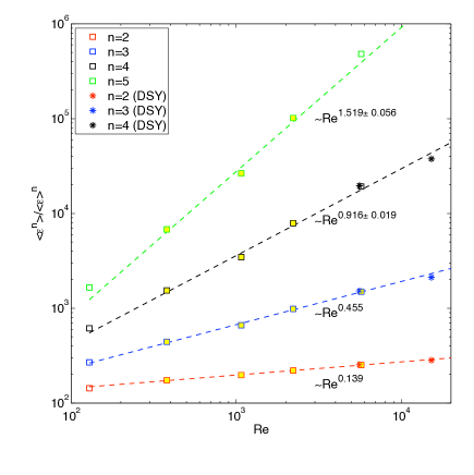
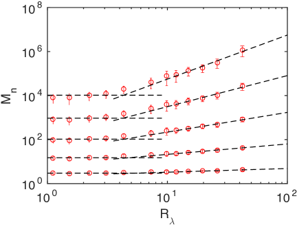
Figure 1: Top panel: Normalized moments $M^{{\cal E}}_{n}=\overline{{\cal E}^{n}}/\overline{{\cal E}}^{n}$ as a function of Reynolds number. Dashed lines: theoretical predictions and numerical simulations of Refs.[4]-[5]; Squares are from Ref.[5] and asterisks from our large DNS data base (see Ref. [6] ); Bottom panel: Transition. The same moments in the low-Re transitional range (present work)

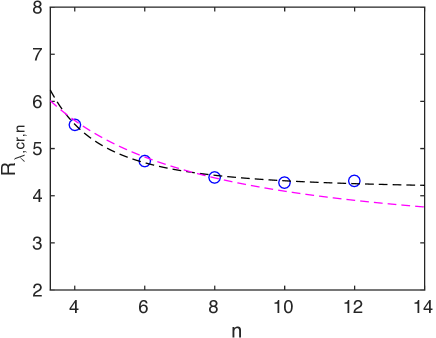
Figure 2: Transitional Reynolds number $R_{\lambda,1}(n)$ of the $n^{th}$ moment of velocity derivative. Blue: numerical simulations of present work. Red: Theoretical prediction with $R^{tr}_{\lambda,n.}=const=8.5$.

Transition between gaussian and anomalous flows. In this paper transition to turbulence is identified with first appearance of non-gaussian anomalous fluctuations of velocity derivatives. The concept is illustrated on the bottom panel of Fig.1, where moments of velocity derivatives from well resolved numerical simulations (described below) are plotted against Reynolds numbers $R_{\lambda}\equiv R_{\lambda,1}\geq 2.$. We can see that transition points of different moments, expressed in terms of $R_{\lambda}\equiv R_{\lambda,1}$, are different and below we denote them $R^{tr}_{\lambda,1}(n)$. It is important that transition point for the lowest order moment $M_{n}$ with $n\approx 1$ has been found at $R_{\lambda}\equiv R_{\lambda,1}\approx 9$ first discovered in Ref.[5] and analytically derived in [9]-[10]. This result can be explained as follows.

In accord with the widely accepted methodology, consider the $R_{\lambda,1}\equiv R_{\lambda}$-dependence of the normalized $n^{th}$ derivative moment $M_{n}$ in a flow driven by a relatively weak force $f$ and large viscosity $\nu$. Then, gradually decreasing viscosity, one reaches the critical magnitude $\nu=\nu_{tr}$ corresponding to $R_{\lambda}^{tr}(n)=R^{-}_{\lambda}(n)$ which is the upper limit for gaussianity of the $n^{th}$ moment. Then, consider the same flow but at a very large Reynolds number (small viscosity). In this, strongly turbulent case, the large-scale low-order moment, $M_{4}$ for example, are dominated by a huge turbulent viscosity $\nu_{T}\propto{\cal E}^{\frac{1}{3}}L^{\frac{4}{3}}$, the largest effective viscosity , accounting for velocity fluctuations at the scales $r<L$ [1]. The effective Reynolds number, corresponding to the integral scale $L$, is $R_{\lambda}^{+}\propto\sqrt{L^{4}/({\cal E}\nu_{T}(L))}(\partial_{x}u)_{rms}^{2}$. This way one reaches the smallest possible Reynolds number $R_{\lambda}\approx 9$ of strongly turbulent (anomalous) flow (see Fig.1). If, in accord with experimental and numerical data, we assume that transition is smooth and at a transition point the Reynolds number is a continuous function meaning that $R_{\lambda}^{-}=R_{\lambda}^{+}$, where $R_{\lambda}^{\pm}$ stand for the magnitudes just above and below transition, we can write:

$$R_{\lambda}^{tr}(4)=\sqrt{\frac{5}{3{\cal E}\nu_{tr}}}v_{rms}^{2}=\sqrt{\frac{5}{3{\cal E}\nu_{T}(L)}}v_{rms}^{2}$$

where effective viscosity of turbulence at the largest (integral) scale calculated in Refs. [9]-[11], is given by

$$\nu_{T}\equiv\nu(L)\approx 0.084\frac{{\cal K}^{2}}{{\cal E}};$$ (8)

where ${\cal K}=v_{rms}^{2}/2$ stands for kinetic energy of velocity fluctuations. Substituting this into the previous relation gives:

$$R_{\lambda}^{tr}(4)=\sqrt{\frac{5}{3{\cal E}\nu}}v_{rms}^{2}=\sqrt{20/(3\times 0.084)}=8.98\approx 9.$$ (9)

extremely close to the outcome of numerical simulations. The coefficient $C_{\mu}=0.084$, derived in [9]-[11] is to be compared with $C_{\mu}=0.09$ widely used in engineering turbulent modeling for half a century [12]. It follows from the relations (5)-(6):

$$R^{tr}_{\lambda}(n)\equiv R^{tr}_{\lambda,1}(n)=(R^{tr}_{\lambda,n})^{\frac{n}{\rho_{2n}}}$$ (10)

The Reynolds number dependence of normalized moments of velocity derivative is shown on Fig.1. The data in the bottom panel of Fig.1 was generated from a new set of simulations at very low Reynolds numbers. As in [6], numerical solutions to Navier-Stokes equations are obtained from Fourier pseudo-spectral calculations with second-order Runge- Kutta integration in time. The turbulence is forced numerically at the large scales, using a combination of independent Ornstein- Uhlenbeck processes with Gaussian statistics and finite-time correlation. Only low wavenumbers modes within a sphere of radius $k_{F}\approx 2$ in wavenumber space are forced. In order to obtain different Reynolds numbers, viscosity is changed accordingly while the forcing at large scales remains constant. In this approach, thus, large scales, and thus the energy flux, remain statistically similar. Resolution is at least $k_{max}\eta\approx 3$ at the highest Reynolds number which was found to produce converged results at the Reynolds numbers investigated here.

Velocity fields are saved at regular time intervals that are sufficiently far apart (of the order of an eddy-turnover time) to ensure statistical independence between them. For each field velocity gradients moments are computed and averaged over space. Ensemble average is computed across these snapshots in time and are used to compute confidence intervals also shown in Fig.1.

The intersection points of curves describing gaussian moments (horizontal dashed lines) and those corresponding to the fully- turbulent anomalous scaling give transitional $R_{\lambda}^{tr}(n)$ for each moment. These are compared to the theoretical prediction of Eq.(10) with $R_{\lambda,n}^{tr}\approx 8.5$ in Fig.2. This result can be understood as follows: in accord with theoretical predictions the transitional Reynolds number $R^{tr}_{\lambda,n}\approx const\approx 9$ in each statistical realization. If $R_{\lambda,1}<R^{tr}_{\lambda}\approx 9$, the transition is triggered by the low -probability violent velocity fluctuations $\overline{(\partial_{x}v_{x})^{n}}^{\frac{1}{n}}>(\partial_{x}x_{x})_{rms}$ coming from the tails of probability density.

It is also interesting to evaluate the limiting, smallest, transitional Reynolds number following (10) in the limit $n\rightarrow\infty$. The relations (5)-(6),(10) give $R_{\lambda}=R^{tr}_{\lambda,1}\rightarrow 2.92$. Evaluated on a popular model $\xi_{n}=\frac{n}{9}+2(1-(\frac{2}{3})^{\frac{n}{3}})$ [13], one readily derives $R^{tr}_{\lambda,1}\rightarrow 3.81$. According to both models, in a flow with $R_{\lambda}\leq 3$, no transition to strong turbulence defined by anomalous scaling of moments of velocity derivatives exist.

Summary and conclusion. In this paper a problem of transition between two different random states has been studied both analytically and numerically. It has been shown that while the gaussian state can be described in terms of the Reynolds number based on the variance of probability density, the description of the intermittent state of strong turbulence requires an infinite number of ”Reynolds numbers” $R_{\lambda,n}$ reflecting the multitude of anomalous scaling exponents of different-order moments ($n$) of velocity derivatives. This novel concept enables one to account for both typical and violent extreme events responsible for emergence of anomalous scaling in the “sub-critical” state when the widely used Reynolds number $R_{\lambda,1}<R^{tr}_{\lambda}$ is small. It has also been demonstrated that, in accord with the theory, the critical $R^{tr}_{\lambda,n}\approx 9$ is independent of $n$. The proposed theory is in a good quantitative agreement with the results of large-scale direct numerical simulations presented above. The role of turbulent bursts in low Reynolds number flows in various physico-chemical processes and the problem of universality will be discussed in future communications.

- (1) 2. C.Lissandrello, K.L.Ekinci & V.Yakhot, J. Fluid Mech, 778, R3 (2015);
- (2) 3. T. Gotoh & T. Nakano , J. Stat Phys. 113, 855 (2003) ;
- (3) 4. V.Yakhot, J.Fluid Mech. 495, 135 (2003);
- (4) 5. J.Schumacher, K.R. Sreenivasan & V. Yakhot, New J. of Phys. 9, 89 (2007);
- (5) 6. D.A. Donzis, P.K. Yeung & K.R. Sreenivasan, Phys.Fluids 20, 045108 (2008);
- (6) 7. P.E. Hamlington, D. Krasnov, T. Boeck & J. Schumacher, J. Fluid. Mech. 701, 419-429 (2012);
- (7) 8. J. Schumacher, J. D. Scheel, D. Krasnov, D. A. Donzis, V. Yakhot & K. R. Sreenivasan, Proc. Natl. Acad. Sci. USA 111, 10961-10965 (2014)
- (8) [9]. V. Yakhot & L. Smith, J. Sci.Comp. 7, 35 (1992);
- (9) 10. V.Yakhot,, Phys.Rev.E, 90, 043019 (2014);
- (10) 11 . V. Yakhot, S.A. Orszag, T. Gatski, S. Thangam & C.Speciale, Phys. Fluids A4, 1510 (1992);
- (11) 12. B.E. Launder,and D.B. Spalding. Mathematical Models of Turbulence, Academic Press, New York (1972); B.E. Launder and D.B. Spaulding, Computer Methods in Applied Mechanics and engineering, 3, 269 (1974).
- (12) 13. Z.S.She & E. Leveque, Phys.Rev.Lett. 72, 336 (1994).