Entanglement phases as holographic duals of anyon condensates

Abstract

Anyon condensation forms a mechanism which allows to relate different topological phases. We study anyon condensation in the framework of Projected Entangled Pair States (PEPS) where topological order is characterized through local symmetries of the entanglement. We show that anyon condensation is in one-to-one correspondence to the behavior of the virtual entanglement state at the boundary (i.e., the entanglement spectrum) under those symmetries, which encompasses both symmetry breaking and symmetry protected (SPT) order, and we use this to characterize all anyon condensations for abelian double models through the structure of their entanglement spectrum. We illustrate our findings with the $\mathbb{Z}_{4}$ double model, which can give rise to both Toric Code and Doubled Semion order through condensation, distinguished by the SPT structure of their entanglement. Using the ability of our framework to directly measure order parameters for condensation and deconfinement, we numerically study the phase diagram of the model, including direct phase transitions between the Doubled Semion and the Toric Code phase which are not described by anyon condensation.

I Introduction

The study of topologically ordered phases, their relation, and the transitions between them has received steadily growing attention in the last decade. Their lack of local order parameters, the dependence of the ground space structure on their topology, and the exotic nature of their anyonic excitations puts them outside the Landau framework of symmetry breaking and local order parameters, and thus asks for novel ways of characterizing and relating different phases, for instance the structure of their ground space or the nature of their non-trivial excitations (anyons), and the way in which those are related throughout different phases.

Anyon condensation has been proposed as a mechanism for relating topological phases bais:anyon-condensation . The main idea is that some mechanism drives a species $a$ of bosonic anyons to condense into the vacuum. This, in turn, forces any anyon $b$ which has non-trivial statistics with $a$ to become confined, as a deconfined $b$ anyon would have non-trivial statistics with the new vacuum, and moreover leads to the identification of anyons which differ by fusion with $a$. At the same time, the relation between anyon types and ground space of a theory suggests that this condensation is accompanied by a change in the ground space structure. The formalism of anyon condensation allows to construct “simpler” anyon models from more rich ones, and suggests to think of the “condensate fraction” of the condensed anyon as an order parameter for a Landau-like description of the phase transition. Yet, it is a priori not clear how such an order parameter should be measured, and existing approaches describe anyon condensation as a breaking of the global symmetry of the quantum group or tensor category underlying the model bais:quantum-sym-breaking ; bais:hopf-symmetry-breaking-jhep ; kitaev:gapped-boundaries ; kong:anyon-condensation-tensor-categories .

Projected Entangled Pair States (PEPS) verstraete:mbc-peps form a natural framework for the local modelling of topologically ordered phases buerschaper:stringnet-peps ; gu:stringnet-peps . They associate to any lattice site a tensor which describes both the physical system at that site, and the way in which it is correlated to the adjacent sites through entanglement degrees of freedom. It has been shown that in PEPS, topological order emerges from a local symmetry constraint on the entanglement degrees of freedom, characterized by a group action (for so-called double models of groups) schuch:peps-sym or more generally by Matrix Product Operators for twisted doubles buerschaper:twisted-injectivity and string-net models sahinoglu:mpo-injectivity ; bultinck:mpo-anyons . In all cases, both ground states and excitations can be modelled from the very same symmetries which characterize the local tensors: Group actions and irreducible representations (irreps) in the former and Matrix Product Operators with suitable endpoints in the latter case schuch:peps-sym ; buerschaper:twisted-injectivity ; sahinoglu:mpo-injectivity ; bultinck:mpo-anyons . Yet, it has been observed that the entanglement symmetry of the tensors is not in one-to-one correspondence with the topological order in the system: By adding a suitable deformation to the fixed point wavefunction, the system can be driven into a phase transition which is consistent with a description in terms of anyon condensation schuch:topo-top ; haegeman:shadows ; marien:fibonacci-condensation ; fernandez:symmetrized-tcode . This raises the question: What is the exact relation between topological phase transitions in tensor networks and anyon condensation, and can we explain this transition “miscroscopically” using the local symmetries in the tensor network description?

In this paper, we derive a comprehensive framework for the explanation, classification, and study of anyon condensation in PEPS. Our framework explains and classifies anyon condensation in terms of the different “entanglement phases” emerging at the boundary under the action of the local entanglement symmetry of the tensor, and provides us with the tools to explicitly study the behavior of order parameters measuring condensation and confimement of anyons. More specifically, we show that the symmetry constraint in the entanglement degrees of freedom of the tensor gives rise to a corresponding “doubled” symmetry in the fixed point of the transfer operator, this is, in the entanglement spectrum at the boundary. Anyon condensation can then be understood in terms of the different phases at the boundary, this is, the symmetry breaking pattern together with a possibly symmetry-protected phase of the residual unbroken symmetry. We give necessary and sufficient conditions for the condensation of anyons in abelian double models in terms of the symmetry at the boundary, and show that this completely classifies all condensation patterns in double models of cyclic groups, giving rise to all twisted $\mathbb{Z}_{N}$ double models. We also show that these conditions allow to independently derive the anyon condensation rules described above, providing a tensor network derivation of these conditions. The central idea is to relate anyon condensation and confinement to the behavior of string order parameters, which in turn can be related to symmetry breaking and symmetry-protected order, and combine this with the constraints arising from the positivity of the boundary state.

We illustrate our framework by discussing all possible phases which can be obtained by condensation from a $\mathbb{Z}_{4}$ double model, which can give rise to Toric Code, Doubled Semion, and trivial phases. Specifically, we show that the Toric Code and Double Semion can exhibit the same symmetry breaking pattern at the boundary, yet are distinguished by different SPT orders, corresponding to the condensation of a charge or a dyon (a combined charge-flux particle), respectively, and thus a different string order parameter. Finally, we apply our framework to numerically study topological phases and the transitions between them along a range of different interpolations. Specifically, the interpretation of condensation and confinement in terms of string order parameters allows us to directly measure order parameters for the different topological phases, namely condensate fractions and order parameters for deconfinement, which allow us to study the nature and order of the phase transitions. Our framework also allows us to set up interpolations between the Toric Code and Double Semion phase, which are a priori not related by anyon condensation, and we find that depending on the nature of the interpolation, we can either find a second-order simultaneous confinement-deconfinement transition, or a first-order transition not characterized by anyon condensation.

The paper is structured as follows: In Sec. II, we introduce PEPS, explain how topological order and topological excitations are modelled within this framework, and define condensation and confinement in PEPS models. Sec. III contains the classification of anyon condensation and confinement through the behavior of the boundary: We start by giving the intuition and the main technical assumption, then derive the conditions imposed by the symmetry structure and positivity of the boundary state, and finally show that this classification gives rise to the well-known anyon condensation rules. In Sec. IV, we apply this classification to the case of $\mathbb{Z}_{N}$ quantum doubles and show that it precisely gives rise to all twisted $\mathbb{Z}_{M}$ double models. Finally, in Sec. V, we illustrate our framework with a detailed discussion of the condensation from a $\mathbb{Z}_{4}$ double, and study the corresponding family of models and the transitions between them numerically.

II Symmetries in PEPS and anyons

In this section, we will first introduce the general PEPS framework. We will then explain how certain symmetries in PEPS naturally lead to objects defined on the entanglement degrees of freedom which behave like anyonic excitations. The natural question is then to understand the conditions under which these objects describe observable anyons, or whether they fail to do so by either leaving the state invariant (condensation) or by evaluating to zero (confinement) in the thermodynamic limit.

We will focus our discussion to the case of abelian groups; however, several of our arguments in fact apply to general groups, and even beyond that for so-called MPO-injective PEPS; we will discuss these aspects in Sec. VI.

II.1 PEPS, parent Hamiltonians, and excitations

Let us start by introducing Projected Entangled Pair States (PEPS). We focus on a translational invariant system on a square lattice with periodic boundary conditions, where we take the system size to infinity. PEPS are constructed from a local tensor $A^{i}_{\alpha\beta\gamma\delta}$, where $i=1,\dots,d$ is the physical index and $\alpha,\beta,\gamma,\delta=1,\dots,D$ are the virtual indices, and $D$ is called the bond dimension. Graphically, they are depicted as a sphere with five legs, one for each index, cf. Fig. LABEL:fig:peps-defa; equivalently, we can consider $A=\sum A^{i}_{\alpha\beta\gamma\delta}|i\rangle\langle\alpha,\beta,\gamma,\delta|$ as a linear map from virtual to physical system. The tensor $A$ is then arranged on a square lattice, Fig. LABEL:fig:peps-defb, and adjacent virtual indices are contracted (i.e., identified and summed over), which is graphically depicted by connecting the corresponding legs. We thus finally obtain a tensor $c_{i_{1}\dots i_{N}}$ which only has physical indices, and thus describes a quantum many-body state $|\Psi\rangle=\sum c_{i_{1}\dots i_{N}}|i_{1},\dots,i_{N}\rangle$. A useful property of PEPS is the possibility to block sites – we can take the tensors on some $k_{1}\times k_{2}$ patch and define them as a new tensor $A^{\prime}$ with correspondingly larger $D$. This allows us to restrict statements about properties of localized regions to fixed-size (e.g., single-site or overlapping $2\times 2$) patches.

To any PEPS, one can naturally associate a family of parent Hamiltonians which have this PEPS as their exact zero-energy ground state perez-garcia:parent-ham-2d ; schuch:peps-sym . Such a Hamiltonian is a sum of local terms $h$, each of which ensures that the state “looks locally correct” on a small patch, i.e., as if it had been built from the tensor $A$ on that patch. This is accomplished by choosing $h\geq 0$ such that $h$ is zero on the physical subspace spanned by the tensors on that patch (for arbitrary virtual boundary conditions) and positive otherwise; note that by choosing a sufficiently large patch, it is always possible to find a non-trivial such Hamiltonian (the dimension of the allowed physical subspace scales with the boundary, while the available degrees of freedom scale with the volume).

Clearly, the global PEPS wavefunction is a zero-energy state and thus a ground state of the parent Hamiltonian $H=\sum h\geq 0$. At the same time, conditions on $A$ are known under which this ground state is unique (in a finite volume) perez-garcia:parent-ham-2d : Specifically, it is sufficient if the map from the virtual to the physical system described by $A$ (possibly after blocking) is injective; equivalently, this means that the full auxiliary space can be accessed by acting on the physical space only, i.e., that one can apply a linear map which “cuts out” a tensor and gives direct access to the auxiliary indices.

Parent Hamiltonians naturally give rise to the notion of localized excitations, this is, states whose energy differs from the ground state only in some local regions. To this end, one replaces some tensors by “excitation tensors” $B$, while keeping the original tensor $A$ everywhere else, cf. Fig. 2a. For injective PEPS, these are in fact the only possible localized excitations, since due to the one-to-one correspondence between virtual and physical system any tensor $B\neq A$ will yield an increased energy w.r.t. the parent Hamiltonian perez-garcia:parent-ham-2d .

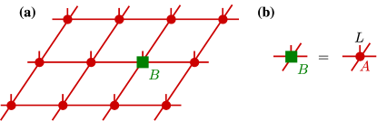
Figure 2: (a) Replacing one tensor by a different tensor $B$ results in a localized excitation, i.e., which is not detected by the parent Hamiltonian anywhere else. (b) An excitation is topologically trivial if $B$ can be obtained from $A$ by acting with a map $L$ on the physical system.

A key question in the context of this work is when an excitation is topologically non-trivial. We will use the following definition: An excitation is topologically trivial exactly if it can be created (with some non-zero probability) by acting locally on the system, i.e., if there exists a linear (not necessarily unitary) map $L$ on the physical system which will create that excitation on top of the ground state, this is, which transforms $A$ to $B$. It is now straightforward to see that for an injective PEPS, all localized excitations (Fig. 2a) are topologically trivial: Injectivity implies that $A$ (as a map from virtual to physical system) has a left-inverse $A^{-1}$, and thus $L:=BA^{-1}$ will act as $LA=B$, i.e., create the desired excitation locally, as shown in Fig. 2b.

II.2 G-injective PEPS and anyonic excitations

Let us now turn towards PEPS which can support topologically non-trivial excitations. To this end, we consider PEPS which are no longer injective, but enjoy a virtual symmetry under some group action,

$$A=A(\bar{U}_{g}\otimes\bar{U}_{g}\otimes U_{g}\otimes U_{g})$$ (1)

with $U_{g}$ a unitary representation of some finite group $G\ni g$; we will denote such tensors as $G$-invariant. Graphically, this is expressed as

$$\raisebox{-20.00003pt}{\includegraphics[scale={0.70}]{figs/ginv-tensor}}\quad,$$ (2)

where we use the convention that matrices act on the indices from left to right and down to up, such that $\bar{U}_{g}$ in Eq. (1) turns into $U_{g}^{\dagger}$. An important property of $G$-invariance is its stability under concatenation: When grouping together several $G$-invariant tensors, the resulting block is still $G$-invariant, as the $U_{g}$ and $U_{g}^{\dagger}$ on the contracted indices exactly cancel out. In the following, we will focus on abelian groups (though various parts of the discussion generalize to the non-abelian case), and denote the neutral element by $e\in G$.

If $G$-invariance is the only symmetry of the tensor $A$, i.e., if $A$ is injective on the subspace left invariant by the symmetry, we call $A$ $G$-injective. The parent Hamiltonians of $G$-injective PEPS have a topological ground space degeneracy and can support anyonic excitations schuch:peps-sym , as we will also discuss in the following. We will generally assume that the tensors are $G$-injective, since otherwise we might be missing a symmetry, likely rendering the discussion incomplete.

II.2.1 Electric excitations

In order to understand how these excitations look like, let us consider again the possible localized excitations w.r.t. the parent Hamiltonian. As we have seen earlier, any state where one tensor has been replaced by a different tensor $B$ is by construction a localized excitation. In the injective case, any such $B$ could be obtained by acting locally on the physical degrees of freedom, rendering the excitation topologically trivial. However, it is easy to see that this is no longer the case for $G$-invariant tensors: Local operations (Fig. 2b) can only produce tensors $B$ which are again $G$-invariant, i.e., transform trivially under the action of the symmetry group, since it is exactly the invariant virtual subspace which is accessible by acting on the physical indices. In contrast, $B$’s which transform non-trivially can no longer be created locally, and thus are topologically non-trivial excitations. It is natural to label these excitations by irreducible representations $\alpha(g)\in\mathbb{C}$ of the abelian symmetry group $G$, this is, we can write

$$B=\sum_{\alpha}B_{\alpha}\ ,$$ (3)

where

This is, any such excitation can be understood as a superposition of excitations with fixed $\alpha$, and we will focus on excitations with a fixed $\alpha$ in the following. These excitations will be denoted as electric excitations with charge $\alpha$. (For non-abelian groups, we would require instead that each $B_{\alpha}$ is supported on the irrep $\alpha$ of the group action.)

It is straightforward to see that for $G$-injective PEPS, the topological part of the excitation is fully characterized by $\alpha$: In case $B_{\alpha}$ itself is injective on the irrep $\alpha$, this is immediate since it can be transformed into any other $B_{\alpha}^{\prime}$ by locally acting on the physical index; in case $B_{\alpha}$ is not injective, the same can be done by acting on a $3\times 3$ block centered around $\alpha$ (due to $G$-injectivity, this allows to access all degrees of freedom at the boundary in the irrep $\alpha$).

In the following, we will focus our attention on electric excitations of the form

(4)

where $R_{\alpha}$ (the yellow diamond) transforms as $R_{\alpha}U_{g}=\alpha(g)U_{g}R_{\alpha}$; the general case will be discussed in Appendix B.

An important point to note about electric excitations is that for any system with periodic boundaries, they must come in pairs (or groups) which together transform trivially under the symmetry action, i.e., have total trivial charge, since otherwise the state would vanish.

II.2.2 Magnetic excitations

For injective PEPS, locally changing tensors was the only way to obtain localized excitations, due to the one-to-one correspondence of physical and virtual system perez-garcia:parent-ham-2d . For $G$-injective PEPS, however, there exist ways to non-locally change the tensor network without creating an excitation, or only creating a localized excitation schuch:peps-sym . To this end, note that Eq. (2) can be reformulated as

  and   (5)

and rotated versions thereof. This has the natural interpretation of the $U_{g}$ and $U_{g}^{\dagger}$ forming strings (symbolized by the dashed blue lines above), which can be freely moved through the lattice (“pulling though condition”). (Whether $U_{g}$ or $U_{g}^{\dagger}$ has to be used depends on the orientation of the string relative to the lattice schuch:peps-sym .) Thus, any string of $U_{g}$’s is naturally invisible to the parent Hamiltonian, as it can be moved away from any patch the parent Hamiltonian acts on. Indeed, if $G$-injectivity holds, one can use the equivalence of physical and virtual system on the invariant subspace to prove that such strings are the only non-local objects which cannot be detected by the parent Hamiltonian schuch:peps-sym . This yields a natural way to build localized excitations by placing a string of $U_{g}$’s with open ends on the lattice, as illustrated in Fig. LABEL:fig:excitation-string-pair: Any such string can only be detected at its endpoints, thereby forming a localized excitation. These excitations are topological by construction, since by acting on the endpoints alone, we are not able to create such a string. At the same time, using $G$-injectivity one can prove that the endpoints can always be detected in a finite system. Thus, we arrive at a second type of topological non-trivial excitations, namely strings of $U_{g}$’s with an endpoint,

$$\includegraphics[scale={0.65}]{figs/dressed-flux-excitation}\quad.$$

(We have followed the notation introduced in Fig. LABEL:fig:excitation-string-pair, where blue dots denote $U_{g}$ or $U_{g}^{\dagger}$, and the dashed blue line highlights the string formed.) Again, $C$ is an arbitrary $G$-invariant tensor which can be used to dress the endpoint with an arbitrary topologically trivial excitation; under blocking, it can always be assumed to only sit on a single site as shown. Again, given periodic boundaries any such string must end in a second anyon (or more generally the strings emerging from several anyons can fuse as long as the corresponding group elements multiply to the identity).

We will denote these excitations as magnetic excitations with flux $g$.

II.2.3 Dyonic excitations

Beyond electric and magnetic excitations, it is also possible to combine the two into a so-called dyon which is of the form

(6)

Note that we have made the choice that the irrep $R_{\alpha}$ sits on the same leg at which the $U_{g}$-string ends. While this choice is arbitrary, it is related to any other endpoint, e.g. one where the string ends on the leg before $R_{\alpha}$, by a local $U_{g}$-string, i.e., a pair of magnetic excitations, which can be created locally and can thus be accounted for by an appropriate choice of $C$, or even incorporated in $R_{\alpha}$.

A general anyonic excitation is thus up to local modifications labeled by a tuple $g$ and $\alpha$; we denote the anyon by ${\llbracket g;\alpha\rrbracket}$, and an anyon string with the two conjugate anyons ${\llbracket g;\alpha\rrbracket}$ and ${\llbracket g;\bar{\alpha}\rrbracket}$ at its endpoints by $S_{{\llbracket g;\bar{\alpha}\rrbracket}-{\llbracket g;\alpha\rrbracket}}$.

II.2.4 Braiding statistics

Let us briefly comment on the braiding statistics of these excitations; we refer to Ref. schuch:peps-sym for details. Any physical procedure for moving anyons will result in the $U_{g}$-string being pulled along the path. Thus, a half-exchange of two identical anyons transforms

(where for simplicity we have set $C=A$, as it transforms trivially). Straightening the string by pulling it through the right excitation requires to commute $g$ with $R_{\alpha}$, which gives rise to a phase $\alpha(g)$; since the resulting two crossing strings are identical to two non-crossing strings, we thus obtain a overall phase of $\alpha(g)$ due to the half exchange.

Similarly, full exchange of two different anyons ${\llbracket g;\alpha\rrbracket}$ and ${\llbracket h;\beta\rrbracket}$ gives rise to two such exchanges, and thus to a mutual statistics $\alpha(h)\beta(g)$ for a full exchange.

We therefore see that the strings defined this way indeed exhibit the same statistics as $D(G)$, the quantum double model of $G$ kitaev:toriccode ; schuch:peps-sym .

II.3 Virtual level vs. observable excitations: Condensation and confinement

II.3.1 Anyon condensation and confinement

It is suggestive to assume that this is the complete picture, and $G$-injective PEPS always exhibit an anyon theory given by the quantum double $D(G)$. However, it has by now been understood that this is not the case schuch:topo-top : By adding a physical deformation $\Lambda$ to the tensor, $A\rightarrow\Lambda A$, one can drive the system towards a product state, eventually crossing a phase transition. E.g., in the toric code this induces string tension (or more precisely loop fugacity), which eventually leads to the breakdown of topological order castelnovo:tc-tension-topoentropy .

This is directly related to the question as to whether the objects which we have just identified as anyonic excitations on the virtual level actually describe observable anyons in the thermodynamic limit, and in the limit of large separation between the individual anyons. While, as we have argued, one can prove schuch:peps-sym that the endpoints of a virtual string $S_{{\llbracket g;\bar{\alpha}\rrbracket}-{\llbracket g;\alpha\rrbracket}}$ correspond to observable excitations, this only applies in a finite volume. However, it is perfectly possible that—depending on the choice of $A$—new behavior emerges in the thermodynamic limit, which is reflected in a non-trivial environment imposed on a virtual anyon string $S_{{\llbracket g;\bar{\alpha}\rrbracket}{{-}\smash{\raisebox{1.959pt}{\!\!\!{$\scriptstyle\ell$}\,}}}{\llbracket g;\alpha\rrbracket}}$ (with $\ell$ the separation between the endpoints) which can prevent it from describing an observable anyonic excitation as $\ell\rightarrow\infty$. This can happen in at least two distinct ways: Either the environment transforms trivially under $S_{{\llbracket g;\bar{\alpha}\rrbracket}{{-}\smash{\raisebox{1.959pt}{\!\!\!{$\scriptstyle\ell$}\,}}}{\llbracket g;\alpha\rrbracket}}$, in which case the PEPS with $S_{{\llbracket g;\bar{\alpha}\rrbracket}{{-}\smash{\raisebox{1.959pt}{\!\!\!{$\scriptstyle\ell$}\,}}}{\llbracket g;\alpha\rrbracket}}$ still describes the ground state, or the environment is orthogonal to $S_{{\llbracket g;\bar{\alpha}\rrbracket}{{-}\smash{\raisebox{1.959pt}{\!\!\!{$\scriptstyle\ell$}\,}}}{\llbracket g;\alpha\rrbracket}}$, in which case the state has norm zero and is thus unphysical.

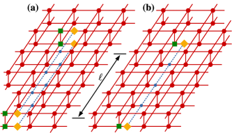
Figure 4: Tensor networks for detecing (a) confinement (the network for the norm of the state evaluates to zero) and (b) condensation (the network for the overlap with the ground state evaluates to non-zero, both as $\ell\rightarrow\infty$) for a general anyon pair of the form Eq. (6).

We will thus distinguish two different ways in which non-trivial virtual excitations $S_{\llbracket g;\alpha\rrbracket}$ might fail to describe observable anyonic excitations:
1. Confinement: The state $|\psi[S_{{\llbracket g;\bar{\alpha}\rrbracket}{{-}\smash{\raisebox{1.959pt}{\!\!\!{$\scriptstyle\ell$}\,}}}{\llbracket g;\alpha\rrbracket}}]\rangle$ of the system with an anyon string does not describe a properly normalizable quantum state, i.e.,

$$\langle\psi[S_{{\llbracket g;\bar{\alpha}\rrbracket}{{-}\smash{\raisebox{1.959pt}{\!\!\!{$\scriptstyle\ell$}\,}}}{\llbracket g;\alpha\rrbracket}}]|\psi[S_{{\llbracket g;\bar{\alpha}\rrbracket}{{-}\smash{\raisebox{1.959pt}{\!\!\!{$\scriptstyle\ell$}\,}}}{\llbracket g;\alpha\rrbracket}}]\rangle\rightarrow 0\mbox{\ as\ }N,\ell\rightarrow\infty\$$ (7)

where first the system size $N$ and then the separation $\ell$ is taken to infinity. The expectation value in Eq. (7) corresponds to the tensor network in Fig. 4a, this is, the expectation value of the string operator $\bar{S}_{{\llbracket g;\bar{\alpha}\rrbracket}{{-}\smash{\raisebox{1.959pt}{\!\!\!{$\scriptstyle\ell$}\,}}}{\llbracket g;\alpha\rrbracket}}\otimes S_{{\llbracket g;\bar{\alpha}\rrbracket}{{-}\smash{\raisebox{1.959pt}{\!\!\!{$\scriptstyle\ell$}\,}}}{\llbracket g;\alpha\rrbracket}}$ in the double layer ket+bra tensor network.
2. Condensation: $|\psi[S_{{\llbracket g;\bar{\alpha}\rrbracket}{{-}\smash{\raisebox{1.959pt}{\!\!\!{$\scriptstyle\ell$}\,}}}{\llbracket g;\alpha\rrbracket}}]\rangle$ is not orthogonal to the ground state $|\psi\rangle$ in the thermodynamic limit,

$$\langle\psi|\psi[S_{{\llbracket g;\bar{\alpha}\rrbracket}{{-}\smash{\raisebox{1.959pt}{\!\!\!{$\scriptstyle\ell$}\,}}}{\llbracket g;\alpha\rrbracket}}]\rangle\neq 0\quad\mbox{as}\quad N,\ell\rightarrow\infty\ ,$$ (8)

i.e., the individual endpoints are not distinguished any more from the ground state by a topological symmetry, and thus differ from it at most in local properties. The corresponding tensor network is shown in Fig. 4b and corresponds to the expectation value of the string operator $\openone\otimes S_{{\llbracket g;\bar{\alpha}\rrbracket}{{-}\smash{\raisebox{1.959pt}{\!\!\!{$\scriptstyle\ell$}\,}}}{\llbracket g;\alpha\rrbracket}}$.

In the remainder of this paper, we will explore the conditions under which condensation and confinement occurs in PEPS models, and provide a classification of the possibly ways in which this can happen.

II.3.2 Condensation, confinement, and string order parameters

In order to understand condensation and confinement of anyons in PEPS models, we need to assess the behavior of overlaps $\langle\psi[\bar{S}_{{\llbracket g^{\prime};\bar{\alpha}^{\prime}\rrbracket}{{-}\smash{\raisebox{1.959pt}{\!\!\!{$\scriptstyle\ell$}\,}}}{\llbracket g^{\prime};\alpha^{\prime}\rrbracket}}]|\psi[S_{{\llbracket g;\bar{\alpha}\rrbracket}{{-}\smash{\raisebox{1.959pt}{\!\!\!{$\scriptstyle\ell$}\,}}}{\llbracket g;\alpha\rrbracket}}]\rangle$, corresponding to string operators $S_{{\llbracket g;\bar{\alpha}\rrbracket}{{-}\smash{\raisebox{1.959pt}{\!\!\!{$\scriptstyle\ell$}\,}}}{\llbracket g;\alpha\rrbracket}}\otimes\bar{S}_{{\llbracket g^{\prime};\bar{\alpha}^{\prime}\rrbracket}{{-}\smash{\raisebox{1.959pt}{\!\!\!{$\scriptstyle\ell$}\,}}}{\llbracket g^{\prime};\alpha^{\prime}\rrbracket}}$ on the virtual level, cf. Fig. 4, in the thermodynamic limit and as $\ell\rightarrow\infty$. In what follows, we will assume $C=C^{\prime}=A$ for simplicity; we discuss how to adapt the arguments to the general case in Appendix B.

It is instrumental to introduce the transfer operator

$$\mathbb{T}:=\raisebox{-50.00008pt}{\includegraphics[scale={0.6}]{figs/transfer-op}}$$

which is a completely positive map (from left to right) acting on a one-dimensional chain of $D$-level systems; if we disregard complete positivity, we can equally think of $\mathbb{T}$ as a map on a 1D chain of $\mathbb{C}^{D}\otimes\mathbb{C}^{D}$ systems. In the following, we will restrict to the case of hermitian $\mathbb{T}$ (corresponding e.g. to a system with combined reflection and time-reversal symmetry), which in particular implies that the left and right fixed points of $\mathbb{T}$ are equal.

Let us now see how the symmetry of the tensor $A$ is reflected in the transfer operator. $G$-invariance of the $A$ is inherited by $\mathbb{T}$, which thus enjoys the symmetries $[\mathbb{T},U^{\otimes N}\otimes\openone]=[\mathbb{T},\openone\otimes\bar{U}^{\otimes N}]=0$ (with $N\rightarrow\infty$ the system size); this is, $\mathbb{T}$ carries an on-site $\bm{G}:=G\times G$ symmetry with representation ${\bm{U}}_{\bm{g}}=U_{g}\otimes U_{g^{\prime}}$, with $\bm{g}\equiv(g,g^{\prime})\in\bm{G}$. The irreps of $\bm{G}$ are given by ${\bm{\alpha}}((h,h^{\prime}))={\bm{\alpha}}((h,e)){\bm{\alpha}}((e,h^{\prime}))\equiv\alpha(h)\bar{\alpha}^{\prime}(h^{\prime})$, where $\alpha(\cdot):={\bm{\alpha}}((\cdot,e))$ and $\alpha^{\prime}(\cdot):={\bar{\bm{\alpha}}}((e,\cdot))$ are irreps of $G$; there is thus a correpondence between irreps of $\bm{G}$ and pairs of irreps of $G$, and we will write $\bm{\alpha}=(\alpha,\alpha^{\prime})$. The trivial irrep will be denoted by $1$. Finally, we define $\bm{S}_{{\llbracket\bm{g};\bar{\bm{\alpha}}\rrbracket}{{-}\smash{\raisebox{1.959pt}{\!\!\!{$\scriptstyle\ell$}\,}}}{\llbracket\bm{g};\bm{\alpha}\rrbracket}}:=S_{{\llbracket g;\bar{\alpha}\rrbracket}{{-}\smash{\raisebox{1.959pt}{\!\!\!{$\scriptstyle\ell$}\,}}}{\llbracket g;\alpha\rrbracket}}\otimes\bar{S}_{{\llbracket g^{\prime};\bar{\alpha}^{\prime}\rrbracket}{{-}\smash{\raisebox{1.959pt}{\!\!\!{$\scriptstyle\ell$}\,}}}{\llbracket g^{\prime};\alpha^{\prime}\rrbracket}}$. Generally, we will stick to the convention that we use boldface letters for objects living on ket+bra.

In terms of the transfer operator, we can now re-express our quantities of interest for condensation and confinement as expectation values of $\bm{S}_{{\llbracket\bm{g};\bar{\bm{\alpha}}\rrbracket}{{-}\smash{\raisebox{1.959pt}{\!\!\!{$\scriptstyle\ell$}\,}}}{\llbracket\bm{g};\bm{\alpha}\rrbracket}}$ in some left and right fixed points $(\rho_{L}|$ and $|\rho_{R})$ of $\mathbb{T}$

$$\langle\psi[S_{{\llbracket g^{\prime};\bar{\alpha}^{\prime}\rrbracket}{{-}\smash{\raisebox{1.959pt}{\!\!\!{$\scriptstyle\ell$}\,}}}{\llbracket g^{\prime};\alpha^{\prime}\rrbracket}}]|\psi[S_{{\llbracket g;\bar{\alpha}\rrbracket}{{-}\smash{\raisebox{1.959pt}{\!\!\!{$\scriptstyle\ell$}\,}}}{\llbracket g;\alpha\rrbracket}}]\rangle=(\rho_{L}|\bm{S}_{{\llbracket\bm{g};\bar{\bm{\alpha}}\rrbracket}{{-}\smash{\raisebox{1.959pt}{\!\!\!{$\scriptstyle\ell$}\,}}}{\llbracket\bm{g};\bm{\alpha}\rrbracket}}|\rho_{R})\;,$$

where we assume $(\rho_{L}|\rho_{R})=1$. [We use round brackets $|\cdot)$ to denote vectors on the joint ket+bra virtual level.] The $|\rho_{\bullet})$ can also be understood as operators acting between ket and bra level, in which case we will denote them by $\rho_{\bullet}$. Specifically, $\rho_{L}\rho_{R}$ has been shown to exactly reproduce the entanglement spectrum of a bipartition of the system cirac:peps-boundaries , and thus any statement about the $\rho_{\bullet}$ translates into a property of the entanglement spectrum. Note that $\bm{S}_{{\llbracket\bm{g};\bar{\bm{\alpha}}\rrbracket}{{-}\smash{\raisebox{1.959pt}{\!\!\!{$\scriptstyle\ell$}\,}}}{\llbracket\bm{g};\bm{\alpha}\rrbracket}}$ is formed exactly by a string of symmetry operations and terminated by irreps of the doubled symmetry group $\bm{G}\equiv G\times G$, i.e., a string order parameter, and it is thus suggestive to understand the condensation and confinement of anyons by studying the possible behavior of string order parameters for the group $\bm{G}$.

III Classification of string order parameters and condensation

The following section presents the core result of the paper: We classify all different behaviors which the string operators $\bm{S}_{{\llbracket\bm{g};\bar{\bm{\alpha}}\rrbracket}{{-}\smash{\raisebox{1.959pt}{\!\!\!{$\scriptstyle\ell$}\,}}}{\llbracket\bm{g};\bm{\alpha}\rrbracket}}$ in a $G$-invariant PEPS can exhibit by relating them to the classification of symmetry-protected (SPT) phases in one dimension, as given by the fixed point of the transfer operator. We start in Sec. III.1 by explaining the intuition why the classification of anyon behaviors should be related to the classification of 1D phases. In Sec. III.2 we explicitly state the technical assumptions made (specifically, the form of the fixed point space). Secs. III.3–III.6 contain the classification: In Sec. III.3, we study the structure of symmetry breaking of the fixed point space and show that the endpoints $\bm{S}_{{\llbracket\bm{g};\bar{\bm{\alpha}}\rrbracket}{{-}\smash{\raisebox{1.959pt}{\!\!\!{$\scriptstyle\ell$}\,}}}{\llbracket\bm{g};\bm{\alpha}\rrbracket}}$ decouple as $\ell\rightarrow\infty$, allowing us to restrict to semi-infinite strings in the following; in Sec. III.4, we derive the constraints imposed by the symmetry breaking on the anyons and show how it allows to decouple anyon pairs; in Sec. III.5, we make the connection between the behavior of anyons and the SPT structure of the fixed points, and in Sec. III.6, we show that there exists an additional non-trivial restriction on the SPTs which can appear as fixed points of $\mathbb{T}$, and thus to the possible anyon behavior, arising from the (complete) positivity of $\mathbb{T}$. Finally, in Sec. III.7, we show that the conditions derived in the preceding sections precisely give rise to the known anyon condensation rules.

III.1 Intuition

Let us first present the intuition behind this classification. To this end, we use that we are interested in gapped phases and thus the system is short-range correlated: This suggests that the fixed point of the transfer operator $\mathbb{T}$ is short range correlated as well, and thus has the same structure as the ground state of a local Hamiltonian with the identical symmetry $[\mathbb{T},{\bm{U}}_{\bm{g}}^{\otimes N}]=0$.

Let us now consider the different phases of such a Hamiltonian. We first restrict to the the regime of Landau theory, where phases are classified by order parameters, i.e., irreps of the symmetry group. Depending on the phase, different irreps will have zero or non-zero expectation values, which implies condensation [for a non-zero expectation value of an irrep $(\alpha,e)$ with $\alpha\neq e$] and confinement [for a vanishing expectation value of an irrep $(\alpha,\alpha)$] of charges, corresponding to broken diagonal or unbroken non-diagonal symmetries, respectively. On the other hand, assuming a mean-field ansatz (which is exact in a long-wavelength limit), we find that strings of group actions either create a domain wall (for a broken symmetry) or act trivially (for an unbroken symmetry), relating the symmetry breaking patterns also to the condensation and confinement of magnons. We thus see that the condensation and confinement of electric and magnetic excitations corresponds to Landau-type symmetry breaking in the fixed point of the transfer operator, as observed in Ref. haegeman:shadows . As we will see in the following, this picture becomes more rich when we go beyond Landau theory and allow for SPT phases: These phases are not captured by mean-field theory and are rather characterized by the behavior or string order parameters, i.e., strings of group actions terminated by order parameters, which give rise to condensation and confinement of dyonic excitations.

III.2 The assumption: Matrix Product fixed points

We start by stating our main technical assumption: The fixed point space of $\mathbb{T}$ (possibly after blocking) is spanned by a set of injective Matrix Product States (MPS), which are related by the action of the symmetry group.

Let us be more specific. Let ${\bm{i}}=(i,i^{\prime})$ denote a joint ket+bra index of the blocked transfer operator. Then, we assume there exists a set of matrices $M^{\bm{i},\bm{c}}$ which describe distinct MPS

$$|\rho_{\bm{c}})=\raisebox{-7.5pt}{\includegraphics[scale={.9}]{figs/Ac_mps}}$$

on a finite chain with periodic boundary conditions. We require that these MPS fulfill the following conditions:

1. The $|\rho_{\bm{c}})$ span the full fixed point space of $\mathbb{T}$. (This is, evaluating any quantity of interest either in the fixed point space of $\mathbb{T}$ or in $\mathrm{span}\{|\rho_{\bm{c}})\}$ yields the same result in the thermodynamic limit.)

2. The $|\rho_{\bm{c}})$ are injective, i.e., $\mathbb{E}_{\bm{c}}^{\bm{c}}$ has a unique eigenvalue with maximal magnitude, where $\mathbb{E}_{\bm{c}}^{\bm{c}^{\prime}}:=\sum_{\bm{i}}M^{{\bm{i}},\bm{c}}\bar{M}^{{\bm{i}},\bm{c}^{\prime}}$ is the mixed transfer operator of the MPS. W.l.o.g., we choose to normalize $M^{{\bm{i}},\bm{c}}$ such that $\lambda_{\mathrm{max}}(\mathbb{E}_{\bm{c}}^{\bm{c}})=1$.

3. For each $\bm{c}$ and $\bm{g}$, there is a $\bm{c}^{\prime}$ such that $\bm{U_{g}}|\rho_{\bm{c}}\rangle=|\rho_{\bm{c}^{\prime}}\rangle$, and for each pair $\bm{c}$, $\bm{c}^{\prime}$, there is a corresponding $\bm{g}$. (Here and in the following, we use $\bm{U_{g}}$ as a shorthand for the global symmetry action ${\bm{U}}_{\bm{g}}^{\otimes N}$ whenever the meaning is clear from the context.)

Note that we make no assumption that the $\rho_{\bm{c}}$ are positive, and in fact in many cases the fixed point space cannot be spanned by positive and injective MPS.

Assumption 1 is the main technical assumption here. Note that to some extent a similar assumption underlies the classification of phases of 1D Hamiltonians chen:1d-phases-rg ; schuch:mps-phases , where the ground space is approximated by MPS as well: While this is motivated by the known result that MPS can approximate ground states of finite systems efficiently hastings:arealaw ; verstraete:faithfully ; schuch:mps-entropies , also in that scenario it is yet unproven whether this rigorously implies that MPS are sufficiently general to classify phases in the thermodynamic limit.

Assumptions 2 and 3 can be replaced by the weaker assumption that the fixed point space is spanned by some MPS, together with the assumption that we are not missing any symmetries. Specifically, given an MPS with periodic boundary conditions, it can be brought into a standard form (possibly involving blocking of sites) where it can be understood as a superposition of distinct injective MPS $|\rho_{\bm{c}})$ (possibly with size-dependent amplitudes) perez-garcia:mps-reps ; cirac:mpdo-rgfp . While the $|\rho_{\bm{c}})$ are not necessarily fixed points of the transfer operator themselves, such as in the case of an antiferromagnet where the transfer operator acts by permuting the $|\rho_{\bm{c}})$, they will be fixed points of the transfer operator obtained after suitable blocking. Since, as we will see in a moment, cross-terms between different $|\rho_{\bm{c}})$ vanish when computing physical quantities of interest, we can instead work with a fixed point space spanned by the $|\rho_{\bm{c}})$ , corresponding to Assumption 2.

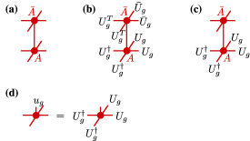
Figure 5: Possible symmetries in the single-site tensor of the transfer operator. (a) Joint ket+bra single-site tensor. (b) Single-layer symmetry, related to topological order, Eq. (1). (c) Double-layer symmetry. (d) Local encoding of a global physical symmetry $u_{g}$ related to the symmetry (c). Degeneracy of the transfer operator under such a joint symmetry implies breaking of the physical symmetry rispler:peps-symmetrybreaking .

Assumption 3 can be justified by requiring that any degeneracy is due to some symmetry of the transfer operator—otherwise, it would be an accidental degeneracy and thus not stable against perturbations. Since the transfer operator has itself a Matrix Product structure, any symmetry of the transfer operator must be encoded locally, i.e., it will show up as a symmetry of the single-site ket+bra object shown in Fig. 5a perez-garcia:inj-peps-syms . There can be two distinct types of such symmetries: Those which act identically on ket and bra layer, shown in Fig. 5b for on-site symmetries, and those which only act on one layer, shown in Fig. 5c. (Symmetries which act on the two layers in distinct ways can be split into a product of the former two symmetries, cf. the argument at the beginning of Sec. III.3.) Symmetries which only act on one layer correspond to topological symmetries of the PEPS tensor, such as those of Eq. (1), and thus need to be incorporated into the description from the very beginning. Symmetries acting identically on ket and bra layer, on the other hand, give rise to a non-trivial physical symmetry action through the identity in Fig. 5d and thus correspond to a global physical symmetry of the system; since their corresponding symmetry sectors are degenerate in the transfer operator, they are susceptible to physical perturbations which lead to symmetry breaking rispler:peps-symmetrybreaking , and we can therefore assume that the system is in one of the symmetry-broken sectors, in which all fixed points are related by the action of the topological symmetry. This in particular includes breaking of translational symmetry, which warrants that we can obtain injective tensors by blocking sites. Note that it is conceivable that different symmetry-broken sectors are described by a different condensation scheme (a simple example can be obtained by coupling different deformations of the system to an Ising model).

III.3 Symmetry breaking structure

In this section, we clarify the symmetry breaking structure of the fixed point space, and show that the relevant expecation values do not depend on which vector in the fixed point space we choose.

To this end, consider the set of $|\rho_{\bm{c}})$ satisfying the three assumptions just laid out. For each $\bm{c}$, let $\bm{H}_{\bm{c}}:=\{\bm{h}\in\bm{G}\,:\;\bm{U}_{\bm{h}}|\rho_{\bm{c}})=|\rho_{\bm{c}})\}$. It is clear that $\bm{H}_{\bm{c}}\subset\bm{G}$ is a subgroup of $\bm{G}$; furthermore, for $G$ abelian $\bm{H}_{\bm{c}}$ is independent of $\bm{c}$, since for any $\bm{h}\in\bm{H}_{\bm{c}}$ and $\bm{g}\in\bm{G}$ s.th. $\bm{U}_{\bm{g}}|\rho_{\bm{c}}\rangle=|\rho_{\bm{c}^{\prime}}\rangle$,

$$|\rho_{\bm{c}^{\prime}}\rangle=\bm{U}_{\bm{g}}|\rho_{\bm{c}}\rangle=\bm{U}_{\bm{g}}\bm{U}_{\bm{h}}|\rho_{\bm{c}}\rangle=\bm{U}_{\bm{h}}\bm{U}_{\bm{g}}|\rho_{\bm{c}}\rangle=\bm{U}_{\bm{h}}|\rho_{\bm{c}^{\prime}}\rangle\ ,$$

and we write $\bm{H}\equiv\bm{H}_{\bm{c}}$.

What is the structure of $\bm{H}$? To this end, consider arbitrary $\gamma_{\bm{c}}$ s.th. $\rho:=\sum\gamma_{\bm{c}}\rho_{\bm{c}}\geq 0$. For any $\bm{h}=(h,h^{\prime})\in\bm{H}$, we have that $\rho=U_{h}\rho U_{h^{\prime}}^{\dagger}$, and thus

$$\rho^{2}=\rho\rho^{\dagger}=(U_{h}\rho U_{h^{\prime}}^{\dagger})(U_{h^{\prime}}\rho U_{h}^{\dagger})=U_{h}\rho^{2}U_{h}^{\dagger}\ ,$$

and thus $[\rho^{2},U_{h}]=0$. Since $\rho\geq 0$, this implies that $[\rho,U_{h}]=0$ as well, or

$$\rho=U_{h}\rho U_{h}^{\dagger}\ ,$$ (9)

and similarly $\rho=U_{h^{\prime}}\rho U_{h^{\prime}}^{\dagger}$. Now choose $\gamma_{\bm{c}}$ s.th. $\rho=\sum\gamma_{\bm{c}}\rho_{\bm{c}}=\mathbb{T^{\infty}}(\openone)$, the fixed point of $\mathbb{T}$ obtained when starting from $\openone$, and pick some $\bm{c}_{0}$. Then, for sufficiently small $\epsilon\geq 0$, $\sigma^{\prime}:=\openone+\epsilon(\rho_{\bm{c}_{0}}+\rho_{\bm{c}_{0}}^{\dagger})\geq 0$ and $\sigma^{\prime\prime}:=\openone+i\epsilon(\rho_{\bm{c}_{0}}-\rho_{\bm{c}_{0}}^{\dagger})\geq 0$, and thus $\rho^{\prime}:=\mathbb{T}^{\infty}(\sigma^{\prime})$ and $\rho^{\prime\prime}:=\mathbb{T}^{\infty}(\sigma^{\prime\prime})$ are both positive fixed points and therefore satisfy Eq. (9), which implies that also $\rho_{\bm{c}_{0}}=\tfrac{1}{2\epsilon}[(\rho^{\prime}-\rho)-i(\rho^{\prime\prime}-\rho)]$ satisfies $\rho_{\bm{c}_{0}}=U_{h}\rho_{\bm{c}_{0}}U_{h}^{\dagger}$. We thus find that whenever $(h,h^{\prime})\in\bm{H}$, we must also have that $(h,h)\in\bm{H}$ and $(h^{\prime},h^{\prime})\in\bm{H}$.

Now consider a general element $(k\ell,k)\in\bm{H}$. Then, $(k,k)\in\bm{H}$, and thus $(\ell,e)=(k\ell,k)\cdot(k,k)^{-1}\in\bm{H}$. It follows that $K\ni k$ and $L\ni\ell$ form groups, and since $(\ell,e)\in\bm{H}\,\Rightarrow(\ell,\ell)\in\bm{H}$, $L\subset K$.

Condition 1

The conserved symmetry $\bm{H}$ is isomorphic to a direct product $K\times L$ with $L\subset K$, where $K$ labels the the diagonal and $L$ the off-diagonal symmetry, i.e., $H\ni\bm{h}=(k\ell,k)$ with $k\in K$ and $\ell\in L$.

To distinguish it from the ket/bra product, we will denote the diagonal/off-diagonal product by $\bm{H}=K\boxtimes L$.

Let us now consider the evaluation of a anyonic string order parameter $\bm{S}_{{\llbracket\bm{g};\bar{\bm{\alpha}}\rrbracket}{{-}\smash{\raisebox{1.959pt}{\!\!\!{$\scriptstyle\ell$}\,}}}{\llbracket\bm{g};\bm{\alpha}\rrbracket}}$ inside general left and right boundary conditions $\sum\lambda_{\bm{c}}^{l/r}|\rho_{\bm{c}})$. This results in a sum over terms of the form

$$O_{\bm{c}}^{\bm{c}^{\prime}}:=\raisebox{-28.00006pt}{\includegraphics[scale={0.6}]{figs/sop_pair_mixed}}\ ,$$ (10)

where we supress the dependency of $O_{\bm{c}}^{\bm{c}^{\prime}}$ on $\bm{\alpha}$ and $\bm{g}$. In case $\bm{c}\neq\bm{c}^{\prime}$, the largest eigenvalue of the mixed transfer operator $\mathbb{E}_{\bm{c}}^{\bm{c}^{\prime}}$ is strictly smaller than one (a straightforward application of Cauchy-Schwarz, see e.g. Lemma 8 of Ref. fernandez-gonzalez:uncle-long ), and thus, $O_{\bm{c}}^{\bm{c}^{\prime}}\rightarrow 0$ exponentially as $N\rightarrow\infty$, i.e., only terms with $\bm{c}=\bm{c}^{\prime}$ survive in the thermodynamic limit. In case $\bm{c}=\bm{c}^{\prime}$, we use that $|\rho_{\bm{c}})=\bm{U}_{\bm{h}}|\rho_{{\bm{c}}_{0}})$ for some fiducial ${\bm{c}}_{0}$ with $\bm{h}\in\bm{G}$, and thus

$$O_{\bm{c}}^{\bm{c}}=\raisebox{-36.0001pt}{\includegraphics[scale={0.6}]{figs/sop_pair_mixed_Uh}}$$ (11)

and since $\bm{U}_{\bm{g}}$ and $\bm{U}_{\bm{h}}$ commute, and the phases from commuting $\bm{U}_{\bm{h}}{\bm{R}_{\bm{\alpha}}}=\bm{\alpha}(\bm{h}){\bm{R}_{\bm{\alpha}}}\bm{U}_{\bm{h}}$ and $\bm{U}_{\bm{h}}{\bm{R}_{\bar{\bm{\alpha}}}}=\bar{\bm{\alpha}}(\bm{h}){\bm{R}_{\bar{\bm{\alpha}}}}\bm{U}_{\bm{h}}$ cancel out, we find that $O_{\bm{c}}^{\bm{c}}=O_{\bm{c}_{0}}^{\bm{c}_{0}}$. We thus find that the expectation value for any string is the same regardless of the boundary conditions, and we will therefore omit the subscript $\bm{c}_{0}$ from now on and write $\rho\equiv\rho_{\bm{c}_{0}}$ and $M\equiv M^{c_{0}}$ (in fact, we will most of the time also omit the label $M$ of the tensor).

After these considerations, we are left with the following question: Given a symmetry $\bm{H}\subset\bm{G}$, $\bm{H}=K\boxtimes L$, and an invariant fixed point $|\rho)$ given by an injective MPS with tensor $M$, what are the the different possible ways in which strings describing the behavior of anyons can behave regarding condensation and confinement.

III.4 Behavior of string order parameters I: Symmetry breaking and decoupling

Let us now consider what happens when we separate the two ends of a string $\bm{S}_{{\llbracket\bm{g};\bar{\bm{\alpha}}\rrbracket}{{-}\smash{\raisebox{1.959pt}{\!\!\!{$\scriptstyle\ell$}\,}}}{\llbracket\bm{g};\bm{\alpha}\rrbracket}}$. Evaluated in the fixed point MPS $|\rho)\equiv|\rho_{\bm{c}_{0}})$, this corresponds to

$$\begin{array}[]{l}(\rho|\bm{S}_{{\llbracket\bm{g};\bar{\bm{\alpha}}\rrbracket}{{-}\smash{\raisebox{1.959pt}{\!\!\!{$\scriptstyle\ell$}\,}}}{\llbracket\bm{g};\bm{\alpha}\rrbracket}}|\rho)=\\[6.00006pt] \hskip 14.22636pt\raisebox{-11.99998pt}{\includegraphics[scale={0.6}]{figs/sop_pair_sep}}\quad.\end{array}\vspace*{1em}$$ (12)

We now distinguish two cases: If $\bm{g}\notin\bm{H}$, then $\bm{U_{g}}^{\otimes N}|\rho_{\bm{c}_{0}}\rangle=|\rho_{\bm{c}^{\prime}}\rangle$ with $\bm{c}^{\prime}\neq\bm{c}_{0}$, and since different representations of an injective MPS are related by a local gauge transformation perez-garcia:mps-reps ; cirac:mpdo-rgfp , it holds that

$$\raisebox{-8.00003pt}{\includegraphics[scale={0.7}]{figs/mps_Ug_Ac0_Acp}}\quad.$$

and thus

$$\raisebox{-32.00002pt}{\includegraphics[scale={0.7}]{figs/mps_top_sym_crossterm}}\quad,$$

and since $\lambda_{\max}(\mathbb{E}^{\bm{c}^{\prime}}_{\bm{c}_{0}})<1$, $(\rho|\bm{S}_{{\llbracket\bm{g};\bar{\bm{\alpha}}\rrbracket}{{-}\smash{\raisebox{1.959pt}{\!\!\!{$\scriptstyle\ell$}\,}}}{\llbracket\bm{g};\bm{\alpha}\rrbracket}}|\rho)\rightarrow 0$ as $\ell\to\infty$. We thus obtain

Condition 2

$(\rho|\bm{S}_{{\llbracket\bm{g};\bar{\bm{\alpha}}\rrbracket}{{-}\smash{\raisebox{1.959pt}{\!\!\!{$\scriptstyle\ell$}\,}}}{\llbracket\bm{g};\bm{\alpha}\rrbracket}}|\rho)\rightarrow 0$ unless $\bm{g}\in\bm{H}$. In particular, all anyons ${\llbracket g;\alpha\rrbracket}$ with $g\not\in K$ are confined.

On the other hand, if $\bm{g}\in\bm{H}$, $\bm{U_{g}}^{\otimes N}|\rho_{\bm{c}_{0}}\rangle=|\rho_{\bm{c}_{0}}\rangle$ and thus there exist $\bm{V}_{\bm{g}}$ such that

$$\raisebox{-10.00002pt}{\includegraphics[scale={0.7}]{figs/mps_Ug_Vg}}\quad,$$ (13)

where $\bm{V}_{\bm{g}}$ forms a projective representation of $\bm{H}$ which can be chosen unitary by a suitable gauge of the MPS sanz:mps-syms . Injectivity of the MPS further implies that its transfer operator $\mathbb{E}\equiv\mathbb{E}_{\bm{c}_{0}}^{\bm{c}_{0}}$ has a unique fixed point

$$\mathbb{E}^{N-\ell-2}=\ \raisebox{-11.99998pt}{\includegraphics[scale={0.6}]{figs/mps_top_fpt}}$$

(w.l.o.g., we choose $\sigma_{R},\sigma_{L}\geq 0$, and normalization implies $\mathrm{tr}[\sigma_{L}\sigma_{R}]=1$), and using Eq. (13), this implies that

$$\raisebox{-11.99998pt}{\includegraphics[scale={0.6}]{figs/mps_top_fpt_sym}}\quad.$$

Also, since $[\mathbb{E},\bm{V}_{\bm{g}}\otimes\bar{\bm{V}}_{\bm{g}}]=0$, uniqueness of the fixed point of $\mathbb{E}$ implies that $\bm{V_{g}}\sigma_{\bullet}\bm{V_{g}}^{\dagger}=\sigma_{\bullet}$, where $\bullet=L,R$, and the ordering of the indices of $\sigma_{\bullet}$ is chosen accordingly. With this, we can rewrite Eq. (12) as

$$(\rho|\bm{S}_{{\llbracket\bm{g};\bar{\bm{\alpha}}\rrbracket}{{-}\smash{\raisebox{1.959pt}{\!\!\!{$\scriptstyle\ell$}\,}}}{\llbracket\bm{g};\bm{\alpha}\rrbracket}}|\rho)\rightarrow\langle\bm{S}_{\llbracket\bm{g};\bm{\bar{\alpha}}\rrbracket}^{*}\rangle\langle\bm{S}_{\llbracket\bm{g};\bm{\alpha}\rrbracket}\rangle$$ (14)

where

$$\langle\bm{S}_{\llbracket\bm{g};\bm{\alpha}\rrbracket}\rangle:=\ \raisebox{-11.99998pt}{\includegraphics[scale={0.6}]{figs/mps_sop_fptring}}\quad,$$ (15)

and correspondingly $\langle\bm{S}_{\llbracket\bm{g};\bm{\bar{\alpha}}\rrbracket}^{*}\rangle$. This implies that the expectation value of any string order parameter decouples into a product of two expectation values corresponding to semi-infinite strings, and in order to study condensation and confinement, it is thus sufficient to to consider the behavior of $\langle\bm{S}_{\llbracket\bm{g};\bm{\alpha}\rrbracket}\rangle$, Eq. (15). In order to highlight the role played by the two layers, we will sometimes also write $\langle S_{\llbracket g;\alpha\rrbracket}\otimes\bar{S}_{\llbracket g^{\prime};\alpha^{\prime}\rrbracket}\rangle:=\langle\bm{S}_{\llbracket\bm{g};\bm{\alpha}\rrbracket}\rangle$, with $\bm{g}=(g,g^{\prime})$, $\bm{\alpha}=(\alpha,\alpha^{\prime})$.

III.5 Behavior of string order parameters II: Symmetry protected phases and group cohomology

We will now study the behavior of string order parameters $\langle\bm{S}_{\llbracket\bm{g};\bm{\alpha}\rrbracket}\rangle$, Eq. (15), with $\bm{g}\in\bm{H}$ more closely and show that they are directly related to the classification of symmetry-protected phases through group cohomology. The crucial point here is that, following Eq. (13), a physical symmetry action $\bm{U}_{\bm{g}}$ can be replaced by a virtual symmetry action $\bm{V}_{\bm{g}}$, where the $V_{\bm{k}}$ form a projective representation of the symmetry group, i.e., $\bm{V}_{\bm{g}}\bm{V}_{\bm{h}}=\omega(\bm{g},\bm{h})\bm{V}_{\bm{gh}}$, where $\omega:\bm{H}\times\bm{H}\rightarrow\mathrm{U}(1)$ is a so-called $2$-cocycle – i.e., it satisfies $\omega(\bm{g},\bm{hk})\omega(\bm{h},\bm{k})=\omega(\bm{g},\bm{h})\omega(\bm{gh},\bm{k})$ due to associativity – which, up to gauge choices $V_{\bm{g}}\sim e^{i\phi_{\bm{g}}}V_{\bm{g}}$ is classified by the second cohomology group $\mathrm{H}^{2}(\bm{H},\mathrm{U}(1))$; this discrete classification of the $\bm{V}_{\bm{g}}$ is what is underlying the classification of symmetry-protected phases in one dimensions pollmann:symprot-1d ; chen:spt-order-and-cohomology ; schuch:mps-phases .

The $2$-cocycle $\omega$ also encodes what happens when we commute $\bm{V}_{\bm{g}}$ and $\bm{V}_{\bm{h}}$:

$$\bm{V}_{\bm{g}}\bm{V}_{\bm{h}}=\omega(\bm{g},\bm{h})\bm{V}_{\bm{gh}}=\omega(\bm{g},\bm{h})\bm{V}_{\bm{hg}}=\frac{\omega(\bm{g},\bm{h})}{\omega(\bm{h},\bm{g})}\bm{V}_{\bm{h}}\bm{V}_{\bm{g}}\ .$$

Here, $\tfrac{\omega(\bm{g},\bm{h})}{\omega(\bm{h},\bm{g})}=:\nu_{\bm{h}}(\bm{g})$ is called the slant product propitius:phd-thesis of $\omega$ with $\bm{h}$; for abelian groups, it forms a one-dimensional representation of $\bm{H}$, $\nu_{\bm{h}}(\bm{g}_{1})\nu_{\bm{h}}(\bm{g}_{2})=\nu_{\bm{h}}(\bm{g}_{1}\bm{g}_{2})$ . Note that we can always construct (non-unique) representations $\gamma$ and $\gamma^{\prime}$ of $G$ such that $\gamma(g)\overline{\gamma^{\prime}(g^{\prime})}=\nu_{\bm{h}}((g,g^{\prime}))$ for $(g,g^{\prime})\in\bm{H}$: To this end, let $\gamma(g):=\nu_{\bm{h}}((g,e))$ for $g\in L$, extend $\gamma$ to a representation of $g\in K$ (formally, this corresponds to an induced representation), and define $\gamma^{\prime}(g):=\overline{\nu_{\bm{h}}((g,g)/\gamma(g)}$; finally, both $\gamma$ and $\gamma^{\prime}$ can be extended independently to representations of $G$.

We will now derive conditions on $\bm{g}$ and $\bm{\alpha}$ under which $\langle\bm{S}_{\llbracket\bm{g};\bm{\alpha}\rrbracket}\rangle$ must be zero and demonstrate how in the remaining cases, it can be made non-zero by an appropriate choice of $\bm{R_{\alpha}}$, and we find that this is in one-to-one correspondence to the inequivalent $2$-cocycles, i.e., elements of $\mathrm{H}^{2}(\bm{H},\mathrm{U}(1))$; the no-go part part of this discussion has been first given in Ref. pollmann:spt-detection-1d in the context of string order parameters for SPT phases. To this end, let us consider an MPS with a specific projective representation $\bm{V}_{\bm{g}}$ with corresponding $\omega(\bm{g},\bm{h})$, and consider a string order parameter $\bm{S}_{\llbracket\bm{g};\bm{\alpha}\rrbracket}$ evaluated in that MPS,

$$\langle\bm{S}_{\llbracket\bm{g};\bm{\alpha}\rrbracket}\rangle=\ \raisebox{-11.99998pt}{\includegraphics[scale={0.6}]{figs/mps_sop_fptring}}\quad.$$ (16)

We now insert a resolution of the identity $\bm{U_{h}}\bm{U_{h}}^{\dagger}$ before $\bm{R_{\alpha}}$ and use $\bm{R_{\alpha}}\bm{U_{h}}={\bm{\alpha}}({\bm{h}})\bm{U_{h}}\bm{R_{\alpha}}$, which gives

We thus find that for $\langle\bm{S}_{\llbracket\bm{g};\bm{\alpha}\rrbracket}\rangle$ to be non-zero, it must hold that $\bm{\alpha}=\nu_{\bm{g}}$, the irreducible representation obtained as the slant product of the $2$-cocycle $\omega$. Conversely, by choosing $\bm{R_{\alpha}}$ such that

(17)

– which is always possible due to the injectivity of $M$ – we have that

i.e., $\bm{R_{\alpha}}$ transforms as ${\bm{\alpha}}\equiv\nu_{\bm{g}}$ on $\bm{H}$ as required, and

$$\langle\bm{S}_{\llbracket\bm{g};\bm{\alpha}\rrbracket}\rangle\!=\raisebox{-11.99998pt}{\includegraphics[scale={0.6}]{figs/Reta_choice_nonzero}}\ =1\,.$$

It remains to see how $\bm{R}_{\alpha}$ transforms under the action of the full symmetry group $\bm{G}$, and more specifically that the construction can be generalized to any irrep $\bm{\alpha}$ of $\bm{G}$ with restriction $\bm{\alpha}|_{\bm{H}}\equiv\nu_{\bm{g}}$; this, together with how to separate $\bm{R}_{\alpha}$ into independent ket and bra actions, is discussed in Appendix A.

We thus see that the behavior of string order parameters is in one-to-one correspondence with the different SPT phases appearing in the fixed point of the transfer matrix: For a given SPT phase, a string order parameter $\langle\bm{S}_{\llbracket\bm{g};\bm{\alpha}\rrbracket}\rangle$ can only be non-zero if $\alpha=\nu_{g}$, and at the same time, it is always possible to set up the endpoint ${\bm{R}}_{\bm{\alpha}}$ of the string order parameter such that $\langle\bm{S}_{\llbracket\bm{g};\bm{\alpha}\rrbracket}\rangle$ actually is non-zero.

Condition 3

A string operator $\bm{S}_{\llbracket\bm{g};\bm{\alpha}\rrbracket}$ with $\langle\bm{S}_{\llbracket\bm{g};\bm{\alpha}\rrbracket}\rangle\neq 0$ exists if and only if $\bm{\alpha}(\bm{h})=\nu_{\bm{g}}(\bm{h})$ for all $\bm{h}\in\bm{H}$, with $\bm{\alpha}((h,h^{\prime}))=\alpha(h)\bar{\alpha}^{\prime}(h^{\prime})$, $\bm{g}=(g,g^{\prime})$, and $\nu_{\bm{g}}(\bm{h})=\omega(\bm{h},\bm{g})/\omega(\bm{g},\bm{h})$, where $\omega$ is the $2$-cocycle classifying the fixed point of the transfer operator.

Clearly, the same derivation for the other endpoint of the string, $\langle\bm{S}_{\llbracket\bm{g};\bm{\bar{\alpha}}\rrbracket}^{*}\rangle$, yields exactly the same condition.

Note that Conditions 2 and 3 together show that the “amount of topological order” – this is, the number of anyons – is related to “symmetry breaking gap” between ket and bra, $|K|/|L|$, where $\bm{H}=K\boxtimes L$: Deconfined anyons ${\llbracket g;\alpha\rrbracket}$ satisfy $(g,g)\in\bm{H}$, i.e., $g\in K$, and $(\alpha,\alpha)=\nu_{(g,g)}$, which fixes $\alpha$ on $L$ and thus leaves $|G|/|L|$ possibilities to extend it to $G$, yielding a total of $|K||G|/|L|$ deconfined anyons. Out of those, pairs ${\llbracket g;\alpha\rrbracket}$ and ${\llbracket gk;\alpha\beta\rrbracket}$ are indistinguishable if $(gk,g)\in\bm{H}$, i.e., $k\in L$, and $(\alpha\beta,\alpha)=\nu_{(gk,g)}$, which fixes $\beta$ on $K$, leaving $|G|/|K|$ possible extensions; the size of each set of indistinguishable anyons is thus $|L||G|/|K|$. The total number of anyons – the ratio of these numbers – is thus $(|K|/|L|)^{2}$, and the total quantum dimension is $|K|/|L|$, the “symmetry breaking gap” between ket and bra.

III.6 Constraints from positivity

The condition that $\langle\bm{S}_{\llbracket\bm{g};\bm{\alpha}\rrbracket}\rangle\neq 0$ iff $\bm{\alpha}=\nu_{\bm{g}}$ (Condition 3) has been derived for a general fixed point of MPO form. However, as we have seen in Sec. III.3, we can w.l.o.g. take the fixed point to be positive semidefinite, which gave rise to the structure of the unbroken symmetry subgroup $\bm{H}$ (Condition 1). As we will see now, positivity induces yet another constraint, namely on the $2$-cocycles realizable in the fixed point.

To this end, consider a positive fixed point $\rho\geq 0$ with an SPT characterized by some $2$-cocycle $\omega:\bm{H}\times\bm{H}\rightarrow\mathbb{C}$, and consider some $g^{\prime}$, $\alpha$, and $\alpha^{\prime}$ such that $\langle\bm{S}_{\llbracket{(e,g^{\prime})};{(\alpha,\alpha^{\prime})}\rrbracket}\rangle\neq 0$. Then, also for the other endpoint $\langle\bm{S}_{\llbracket{(e,g^{\prime})};{(\alpha,\alpha^{\prime})}\rrbracket}^{*}\rangle\neq 0$, and thus [following Eq. (14)]

$$0 <\big{|}(\rho|\bm{S}_{{\llbracket(e,g^{\prime});\overline{(\alpha,\alpha^{\prime})}\rrbracket}{{-}\smash{\raisebox{1.959pt}{\!\!\!{$\scriptstyle\ell$}\,}}}{\llbracket\bm{(}e,g^{\prime});\bm{(}\alpha,\alpha^{\prime})\rrbracket}}|\rho)\big{|}^{2}$$

$$=\big{|}\mathrm{tr}[S_{{\llbracket e;\bar{\alpha}\rrbracket}{{-}\smash{\raisebox{1.959pt}{\!\!\!{$\scriptstyle\ell$}\,}}}{\llbracket e;\alpha\rrbracket}}\rho\bar{S}_{{\llbracket g^{\prime};\bar{\alpha}^{\prime}\rrbracket}{{-}\smash{\raisebox{1.959pt}{\!\!\!{$\scriptstyle\ell$}\,}}}{\llbracket g^{\prime};\alpha^{\prime}\rrbracket}}\rho]\big{|}^{2}$$

$$=\big{|}\mathrm{tr}[(\sqrt{\rho}S_{{\llbracket e;\bar{\alpha}\rrbracket}{{-}\smash{\raisebox{1.959pt}{\!\!\!{$\scriptstyle\ell$}\,}}}{\llbracket e;\alpha\rrbracket}}\sqrt{\rho})\,(\sqrt{\rho}\bar{S}_{{\llbracket g^{\prime};\bar{\alpha}^{\prime}\rrbracket}{{-}\smash{\raisebox{1.959pt}{\!\!\!{$\scriptstyle\ell$}\,}}}{\llbracket g^{\prime};\alpha^{\prime}\rrbracket}}\sqrt{\rho})]\big{|}^{2}$$

$$\stackrel{{\scriptstyle(*)}}{{\leq}}\mathrm{tr}[(\sqrt{\rho}S_{{\llbracket e;\bar{\alpha}\rrbracket}{{-}\smash{\raisebox{1.959pt}{\!\!\!{$\scriptstyle\ell$}\,}}}{\llbracket e;\alpha\rrbracket}}\sqrt{\rho})(\ldots)^{\dagger}]$$

$$\hskip 60.00009pt\times\mathrm{tr}[(\sqrt{\rho}\bar{S}_{{\llbracket g^{\prime};\bar{\alpha}^{\prime}\rrbracket}{{-}\smash{\raisebox{1.959pt}{\!\!\!{$\scriptstyle\ell$}\,}}}{\llbracket g^{\prime};\alpha^{\prime}\rrbracket}}\sqrt{\rho})(\ldots)^{\dagger}]$$

$$=(\rho|\bm{S}_{{\llbracket(e,e);\overline{(\alpha,\alpha)}\rrbracket}{{-}\smash{\raisebox{1.959pt}{\!\!\!{$\scriptstyle\ell$}\,}}}{\llbracket\bm{(}e,e);\bm{(}\alpha,\alpha)\rrbracket}}|\rho)$$

$$\hskip 60.00009pt\times(\rho|\bm{S}_{{\llbracket(g^{\prime},g^{\prime});\overline{(\alpha^{\prime},\alpha^{\prime})}\rrbracket}{{-}\smash{\raisebox{1.959pt}{\!\!\!{$\scriptstyle\ell$}\,}}}{\llbracket\bm{(}g^{\prime},g^{\prime});\bm{(}\alpha^{\prime},\alpha^{\prime})\rrbracket}}|\rho)\ ,$$

where we have used Cauchy-Schwarz in $(*)$ [here, $(\ldots)$ denotes the preceding term]. Following Eq. (14), this implies $\langle\bm{S}_{\llbracket{(e,e)};{(\alpha,\alpha)}\rrbracket}\rangle\neq 0$, and thus (from Condition 3) $\alpha(h)=\alpha(h)\bar{\alpha}(e)=\nu_{(e,e)}((h,e))\equiv 1$ for $(h,e)\in\bm{H}$. At the same time, $\langle\bm{S}_{\llbracket{(e,g^{\prime})};{(\alpha,\alpha^{\prime})}\rrbracket}\rangle\neq 0$ implies that $\alpha(h)=\alpha(h)\bar{\alpha}^{\prime}(e)=\nu_{(e,g^{\prime})}((h,e))$, and thus

$$1=\nu_{(e,g^{\prime})}((h,e))=\frac{\omega((h,e),(e,g^{\prime}))}{\omega((e,g^{\prime}),(h,e))}\ ,$$

i.e.:

Condition 4

The projective representations of ket and bra symmetry actions must commute,

$$\bm{V}_{(g,e)}\bm{V}_{(e,g^{\prime})}=\bm{V}_{(e,g^{\prime})}\bm{V}_{(g,e)}\ ,$$ (18)

or $\nu_{(g,e)}((e,g^{\prime}))=1$, where $(g,e),(e,g^{\prime})\in\bm{H}$.

III.7 Anyon condensation rules

Let us now show that the Conditions 1–4 exactly give rise to the anyon condensation rules mentioned in the introduction:

1. Only self-bosons can condense.

2. Anyons become confined if and only if they have mutual non-bosonic statistics with some condensed anyon.

3. Non-confined anyons which differ by a condensed anyon become indistinguishable.

III.7.1 Only self-bosons can condense.

Consider a condensed anyon ${\llbracket g;\alpha\rrbracket}$, $\langle\bm{S}_{\llbracket{(g,e)};{(\alpha,1)}\rrbracket}\rangle\neq 0$. This requires $(g,e)\in\bm{H}=K\boxtimes L$, i.e., $g\in L$, and moreover $\alpha(h)=\nu_{(g,e)}((h,h^{\prime}))\ \forall\,(h,h^{\prime})\in\bm{H}$, and thus $\alpha(g)=\nu_{(g,e)}((g,e))=1$, i.e., ${\llbracket g;\alpha\rrbracket}$ is a self-boson.

III.7.2 Anyons become confined if and only if they have mutual non-bosonic statistics with some condensed anyon.

Let us first show that an unconfined anyon ${\llbracket k;\beta\rrbracket}$, $\langle\bm{S}_{\llbracket{(k,k)};{(\beta,\beta)}\rrbracket}\rangle\neq 0$, must have mutual bosonic statistics with all condensed anyons ${\llbracket g;\alpha\rrbracket}$, $\langle\bm{S}_{\llbracket{(g,e)};{(\alpha,1)}\rrbracket}\rangle\neq 0$. $\langle\bm{S}_{\llbracket{(k,k)};{(\beta,\beta)}\rrbracket}\rangle\neq 0$ implies $k\in K$ and $\beta(h)\overline{\beta(h^{\prime})}=\nu_{(k,k)}((h,h^{\prime}))$ for $(h,h^{\prime})\in\bm{H}$, i.e., $\beta(h)=\nu_{(k,k)}((h,e))$ for $h\in L$. On the other hand, $\langle\bm{S}_{\llbracket{(g,e)};{(\alpha,1)}\rrbracket}\rangle\neq 0$ implies $(g,e)\in\bm{H}$, i.e., $g\in L$, and $\alpha(h)=\nu_{(g,e)}((h,h))$ for $h\in K$. We thus have that

$$\alpha(k)\beta(g)=\nu_{(g,e)}((k,k))\nu_{(k,k)}((g,e))=1\ ,$$

since $\nu_{\bm{g}}(\bm{h})\nu_{\bm{h}}(\bm{g})=1$.

Conversely, consider a confined anyon ${\llbracket k;\beta\rrbracket}$, $\langle\bm{S}_{\llbracket{(k,k)};{(\beta,\beta)}\rrbracket}\rangle=0$: we will show that this implies the existence of a condensed anyon ${\llbracket g;\alpha\rrbracket}$, $\langle\bm{S}_{\llbracket{(g,e)};{(\alpha,1)}\rrbracket}\rangle\neq 0$, which has mutual non-bosonic statistics, $\alpha(k)\beta(g)\neq 1$, by explicitly constructing such an anyon ${\llbracket g;\alpha\rrbracket}$. $\langle\bm{S}_{\llbracket{(k,k)};{(\beta,\beta)}\rrbracket}\rangle=0$ implies that either (i) $k\notin K$ or (ii) there exists $(h,h^{\prime})\in\bm{H}$ s.th. $\beta(h)\overline{\beta(h^{\prime})}\neq\nu_{(k,k)}((h,h^{\prime}))$.

Let us first consider case (i), $k\notin K$. Let $g=e$ [thus $(g,e)\in\bm{H}$], and choose an irrep $\alpha$ of $G$ s.th. $\alpha(h):=\nu_{(g,e)}((h,h^{\prime}))=\nu_{(e,e)}((h,h^{\prime}))\equiv 1$ for $(h,h^{\prime})\in\bm{H}$ – this is, ${\llbracket g;\alpha\rrbracket}$ is condensed. On the other hand, since $k\notin K$ we can always choose $\alpha$ s.th. $\alpha(k)\neq 1$ (as the extension of the irrep from $K$ to $G$ is non-unique), and thus, $\alpha(k)\beta(g)\neq 1$, i.e., the anyons have mutual non-bosonic statistics.

Now consider case (ii): $k\in K$, but there exists some $(h_{0},h_{0}^{\prime})\in\bm{H}$ s.th. $\beta(h_{0})\overline{\beta(h_{0}^{\prime})}\neq\nu_{(k,k)}((h_{0},h_{0}^{\prime}))$. Define $g:=h_{0}h_{0}^{\prime-1}\in L$. Since hermiticity implies $\nu_{(k,k)}((h,e))=\overline{\nu_{(k,k)}((e,h))}$ (as can be shown by relating $\nu_{(k,k)}$ to the behavior of string order parameters) and thus $\nu_{(k,k)}((h,h))=\nu_{(k,k)}((h,e))\nu_{(k,k)}((e,h))=1$, we have that

$$\beta(g) =\beta(g)\beta(h_{0}^{\prime})\overline{\beta(h_{0}^{\prime})}=\beta(h_{0})\overline{\beta(h_{0}^{\prime})}$$

$$\neq\nu_{(k,k)}((h_{0},h_{0}^{\prime}))=\nu_{(k,k)}((g,e))\nu_{(k,k)}((h_{0}^{\prime},h_{0}^{\prime}))$$

$$=\nu_{(k,k)}((g,e))\ .$$

Further, let $\overline{\alpha^{\prime}(h^{\prime})}:=\nu_{(g,e)}((e,h^{\prime}))\equiv 1$ for $h\in L$, and extend it to the trivial irrep $\alpha^{\prime}\equiv 1$ of $G$. Then, $\alpha(h):=\nu_{(g,e)}((h,h))/\overline{\alpha^{\prime}(h)}$, $h\in K$, can be extended to an irrep $\alpha$ of $G$ s.th. $\alpha(h)=\alpha(h)\overline{\alpha^{\prime}(h^{\prime})}=\nu_{(g,e)}((h,h^{\prime}))$ for all $(h,h^{\prime})\in\bm{H}$, i.e., ${\llbracket g;\alpha\rrbracket}$ is condensed. Finally, $\alpha(k)\beta(g)\neq\nu_{(g,e)}((k,k))\nu_{(k,k)}((g,e))=1$, i.e., ${\llbracket g;\alpha\rrbracket}$ and ${\llbracket k;\beta\rrbracket}$ have mutual non-bosonic statistics.

III.7.3 Non-confined anyons which differ by a condensed anyon become indistinguishable.

Let ${\llbracket g;\alpha\rrbracket}$ be condensed, i.e., $g\in L$ and $\alpha(h)=\nu_{(g,e)}((h,h^{\prime}))\ \forall(h,h^{\prime})\in\bm{H}$, and ${\llbracket k;\beta\rrbracket}$ unconfined, $k\in K$ and $\beta(h)\overline{\beta(h^{\prime})}=\nu_{(k,k)}((h,h^{\prime}))\ \forall(h,h^{\prime})\in\bm{H}$. Then, $(gk,k)\in\bm{H}$, and

$$\alpha(h)\beta(h)\overline{\beta(h^{\prime})} =\nu_{(g,e)}((h,h^{\prime}))\nu_{(k,k)}((h,h^{\prime}))$$

$$=\overline{\nu_{(h,h^{\prime})}((g,e))}\overline{\nu_{(h,h^{\prime})}((k,k))}$$

$$=\overline{\nu_{(h,h^{\prime})}((gk,k))}=\nu_{(gk,k)}((h,h^{\prime}))\ ,$$

i.e., the anyons ${\llbracket k;\beta\rrbracket}$ and ${\llbracket gk;\alpha\beta\rrbracket}$ become indistinguishable.

IV Anyon condensation in $D(\mathbb{Z}_{N})$ and twisted double models

We will now show that in the case of cyclic groups, $G=\mathbb{Z}_{N}$, this allows for a full classification of all condensation patterns, and that these condensation patterns give rise exactly to all twisted quantum doubles $D^{\omega_{3}}(\mathbb{Z}_{M})$, where the twist $\omega_{3}$ is given by a $3$-cocycle of $\mathbb{Z}_{M}$ . In what follows, we will write the groups additively with neutral element zero, and addition is understood modulo the order of the group.

IV.1 Allowed phases at the boundary

Let us first study the effect of the above conditions on the possible SPT phases at the boundary, and thus the possible condensation patterns. As we have seen, the symmetry $\bm{G}=\mathbb{Z}_{N}\times\mathbb{Z}_{N}$ of the transfer operator is broken down to a symmetry $\bm{H}=\mathbb{Z}_{qt}\boxtimes\mathbb{Z}_{q}=\{(g,g+th)\,:\,g=0,\dots,qt-1,\,h=0,\dots,q-1\}$. Let us now consider the restriction imposed by Eq. (18) on the second cohomology classification of the projective representations of $\bm{H}$, $\mathrm{H}^{2}(\bm{H},\mathrm{U}(1))=\mathbb{Z}_{q}$ propitius:phd-thesis . To this end, given an element $n\in\mathrm{H}^{2}(\bm{H},\mathrm{U}(1))$, $n=0,\dots,q-1$, we choose a projective representation

$$\bm{V}_{(g,g)}=X^{g}\mbox{\ and\ }\bm{V}_{(ht,0)}=Z^{hn}\ ,$$ (19)

of $\bm{H}$, $g=0,\dots,qt-1$, $h=0,\dots,q-1$, where $X$ and $Z$ are such that $ZX=\mu XZ$, $\mu=\exp(2\pi i/q)$ (e.g. $X$ a cyclic shift and $Z$ a diagonal $q\times q$ matrix), and where $V_{(g+ht,g)}:=V_{(g,g)}V_{(ht,0)}$. It is straightforward to check that these yield $q$ inequivalent (and thus all) projective representation, e.g. by comparing the gauge-invariant commutator $\omega((t,0),(1,1))/\omega((1,1),(t,0))=\mu^{n}$. We now have that $V_{(0,h^{\prime}t)}=V_{(h^{\prime}t,h^{\prime}t)}V_{((q-h^{\prime})t,0)}$ and thus Eq. (18) reads

$$V_{(ht,0)}\,V_{(h^{\prime}t,h^{\prime}t)}V_{((q-h^{\prime})t,0)}=V_{(h^{\prime}t,h^{\prime}t)}V_{((q-h^{\prime})t,0)}\,V_{(ht,0)}$$

which using Eq. (19) is equivalent to $\mu^{hn\cdot h^{\prime}t}=1$, or (since $h$ and $h^{\prime}$ are arbitrary) $\mu^{nt}=1$. This is the case whenever $nt$ is a multiple of $q$, i.e., $n=k\tfrac{q}{\mathrm{gcd}(t,q)}$. Since at the same time, $0\leq n<q$, we find that $k=0,1,\dots,\mathrm{gcd}(t,q)-1$. This is, out of the $q$ different SPT phases under the symmetry group $\bm{H}$, only $\mathrm{gcd}(t,q)$ are allowed due to positivity constraints.

IV.2 Explicit construction of all twisted $\mathbb{Z}_{t}$ doubles and completeness of classification for $\mathbb{Z}_{N}$

We will now show that for cyclic groups, this classification is complete. To this end, we will first show how to obtain all twisted quantum doubles of $\mathbb{Z}_{t}$ by anyon condensation from a $\mathbb{Z}_{N}$ double, and subsequently use this construction to derive explicit PEPS models for all cases consistent with Conditions 1–4.

IV.2.1 Twisted doubles of $\mathbb{Z}_{t}$ from anyon condensation

In the following, we will describe how to construct all so-called twisted quantum doubles $D^{\omega_{r}}(\mathbb{Z}_{t})$ of $\mathbb{Z}_{t}$ by anyon condensation from a quantum double of some $\mathbb{Z}_{N}$, and derive the structure of the SPT at the boundary. Here, $\omega_{r}\equiv\omega_{r}(g,h,\ell)$ is a so-called $3$-cocycle, labelled by an element $r$ of third cohomology group $\mathrm{H}^{3}(\mathbb{Z}_{t},\mathrm{U}(1))=\mathbb{Z}_{t}$, $r=0,\dots,t-1$. We will just state the corresponding results in the main text and postpone the proofs to Appendix C; for more details on twisted double models and $3$-cocycles, we refer the reader to the appendix or Ref. propitius:phd-thesis .

Let $r=0,\dots,t-1$ label an element of $\mathrm{H}^{3}(\mathbb{Z}_{t},\mathrm{U}(1))=\mathbb{Z}_{t}$, set $q=t/\text{gcd}(t,r)$, and let $N:=qt$. We now define tensors with non-zero elements

$$M(a):=\sqrt{\frac{q}{t}} \begin{split}\includegraphics{figs/plaatjes2mod}\end{split}\ \omega(a,g,h-g_{0})\ \ ,$$ (20)

$$N(a):=\sqrt{\frac{q}{t}} \begin{split}\includegraphics{figs/plaatjes3mod}\end{split}\ \overline{\omega(a,g,h-g_{0})}$$ (21)

for $a=0,\dots,t-1$. Here, the range of the thick vertical indices is $0,\dots,t-1$ and that of the thin (horizontal and vertical) indices is $0,\dots,q-1$, and $h=0,\dots,q-1$, $g=0,\dots,t-1$, and $g_{0}=g\,\mathrm{mod}\,q$. Depending on the index, variables are understood modulo $t$ or $q$. The $3$-cocycle $\omega\equiv\omega_{r}$ is defined by

$$\omega(a,g,d)=\exp\left[\frac{2\pi ird}{t^{2}}(a+g-(a+g)\,\mathrm{mod}\,t)\right]\ ,$$

where there is no modular arithmetics in the exponential except for the $\mathrm{mod}\>t$. Eqs. (20,21) determine the amplitude of all non-zero elements of $M(a)$ and $N(a)$, respectively, while all tensor elements inconsistent with the labels of the indices are zero.

The PEPS tensor for the model is now defined as

$$A=\frac{t}{q^{2}}\sum_{a}\ \raisebox{-30.00005pt}{\includegraphics[scale={0.8}]{figs/plaatjes4-crop}}\quad,$$

where the inner legs correspond to the physical and the outer legs to the virtual indices. As we show in Appendix C.1, the PEPS defined by this model describes a twisted $\mathbb{Z}_{t}$ double model with twist $\omega$. As also shown in the appendix, $A$ satisfies $A^{\dagger}=A=A^{2}$, which implies that $AA^{\dagger}=A$ and thus the transfer operator is of the form

$$\begin{split}\includegraphics{figs/plaatjes16-crop}\end{split}\ \ ,$$ (22)

where the second equality holds since

$$\begin{split}\includegraphics{figs/plaatjes19-crop}\end{split}\ \delta_{ab}\ \ .$$

We thus find that the left and right fixed points of the transfer operator are again described by the same tensor. As it turns out, for any fixed $a$ they describe an injective MPS, and thus, the boundary exhibits $t$ symmetry broken sectors labelled by $a=0,\dots,t-1$.

The tensor $A$ has a $\mathbb{Z}_{qt}$ symmetry with generator $S_{(i_{1},i_{2}),(j_{1},j_{2})}=\delta_{i_{1}+1,j_{1}}\delta_{i_{2}+1,j_{2}}\omega(1,i_{1},i_{2}-i_{1})$ (with $i_{1}$, $j_{1}$ $\mathrm{mod}\,t$ and $i_{2}$, $j_{2}$ $\mathrm{mod}\,q$), which follows from the local condition

$$\raisebox{-3.00003pt}{\includegraphics{figs/plaatjes18-crop}}\quad,$$ (23)

where $U_{ij}\equiv U(a)_{ij}=\delta_{ij}\overline{\omega(1,a,i)}$. Together with its “twin” equation

$$\raisebox{-18.00005pt}{\includegraphics{figs/plaatjes17-crop}}\quad,$$ (24)

$V_{ij}\equiv V(a)_{ij}=e^{i\phi_{a}}\omega(1,a-1,i)\delta_{i,j-1}$, Eq. (23) allows us to verify that the symmetry $\mathbb{Z}_{qt}\times\mathbb{Z}_{qt}$ in the fixed point [Eq. (22)] is broken to $\mathbb{Z}_{qt}\boxtimes\mathbb{Z}_{q}$, with generators $G_{1}=S\otimes S^{\dagger}$ and $G_{2}=S^{t}\otimes\openone$. The element $n\in\mathrm{H}^{2}(\mathbb{Z}_{qt}\boxtimes\mathbb{Z}_{q},\mathrm{U}(1))=\mathbb{Z}_{q}$ labelling the virtual symmetry action – determined by the commutation relation of the virtual representations $P_{1}(a)=U(a)V(a+1)$ and $P_{2}(a)=\prod_{i=a}^{a+t-1}U(i)$ of $G_{1}$ and $G_{2}$ – is given by $n=\tfrac{rq}{t}$.

Overall, given $t$ and $r=0,\dots,t-1$, and $q=t/\mathrm{gcd}(t,r)$, we thus have constructed a PEPS with bond dimension $qt$ and virtual $\mathbb{Z}_{qt}$ symmetry which describes a twisted $\mathbb{Z}_{t}$ quantum double with twist $r\in\mathrm{H}^{3}(\mathbb{Z}_{t},\mathrm{U}(1))=\mathbb{Z}_{t}$. In the fixed point of the transfer operator, the symmetry is broken down to $\mathbb{Z}_{qt}\boxtimes\mathbb{Z}_{q}$, and the cocycle $n\in\mathrm{H}^{2}(\mathbb{Z}_{qt}\boxtimes\mathbb{Z}_{q},\mathrm{U}(1))=\mathbb{Z}_{q}$ characterizing the virtual symmetry action in the fixed point is given by $n=\tfrac{rq}{t}$.

IV.2.2 Completeness of the Conditions 1–4

Let us now show that this construction allows us to obtain PEPS models for cyclic $G$ for any case compatible with Conditions 1–4. Concretely, those conditions imply that given a virtual symmetry $\mathbb{Z}_{N}$ in the tensor, it can be broken down to any $\mathbb{Z}_{qt}\boxtimes\mathbb{Z}_{q}$ symmetry where $qt|N$ (“$|$” denotes “divides”), and furthermore, the label $n$ of the cocycle characterizing the fixed points must be a multiple of $\tfrac{q}{\mathrm{gcd}(q,t)}$, $n=k\tfrac{q}{\mathrm{gcd}(q,t)}$.

To this end, define $q^{\prime}:=\mathrm{gcd}(q,t)$, and let $\alpha=q/q^{\prime}$, $n^{\prime}=n/\alpha=k\tfrac{q/\alpha}{\mathrm{gcd}(q,t)}=k=0,\dots,q^{\prime}-1$. Next, let $\beta=\mathrm{gcd}(n^{\prime},q^{\prime})$, and define $n^{\prime\prime}=n^{\prime}/\beta$ and $q^{\prime\prime}=q^{\prime}/\beta$. With $\gamma=\alpha\beta$, we then have that $q=\gamma q^{\prime\prime}$ and $n=\gamma n^{\prime\prime}$. Since $q^{\prime\prime}|q^{\prime}$ and $q^{\prime}|t$, $x:=t/q^{\prime\prime}$ is integer. Then, the construction for the twisted double with $\tilde{t}=t=xq^{\prime\prime}$ and twist $\tilde{r}=xn^{\prime\prime}$ described in the preceding section yields

$$\tilde{q}=\frac{t}{\mathrm{gcd}(\tilde{r},t)}=\frac{xq^{\prime\prime}}{\mathrm{gcd}(xn^{\prime\prime},xq^{\prime\prime})}=\frac{q^{\prime\prime}}{\mathrm{gcd}(n^{\prime\prime},q^{\prime\prime})}=q^{\prime\prime}\ ,$$

and the $2$-cocycle of the fixed point is characterized by $\tilde{n}=\tfrac{\tilde{r}\tilde{q}}{t}=\tfrac{xn^{\prime\prime}q^{\prime\prime}}{xq^{\prime\prime}}=n^{\prime\prime}$.

We thus know how to create a model with parameters $t$, $q^{\prime\prime}=q/\gamma$, and $n^{\prime\prime}=n/\gamma$; let us denote its tensor by $A^{i}_{k_{1},k_{2},k_{3},k_{4}}$, with $k_{s}=0,\dots,q^{\prime\prime}t-1$, and the generator of the $\mathbb{Z}_{q^{\prime\prime}t}$ symmetry by $S$; w.l.o.g., we choose a basis $|k_{s})$ such that $S=\sum|k+1)(k|$. We will now show how from this model, we can create a PEPS with parameters $t$, $q$, and $n$, and overall symmetry $\mathbb{Z}_{M}$ with $M=qt$. (In a second step, we will then generalize this to any $\mathbb{Z}_{N}$ with $qt|N$.) To this end, we extend the bond space to a $M=\gamma(q^{\prime\prime}t)$-dimensional space, $k_{s}\leadsto(\ell_{s},k_{s})$, $\ell_{s}=0,\dots,\gamma-1$, and construct the new tensor $\tilde{A}$ by tensoring each virtual index of $A$ independently with an equal weight superposition of all $|\ell_{s})$, i.e.,

$$\tilde{A}^{i}_{(\ell_{1},k_{1}),(\ell_{2},k_{2}),(\ell_{3},k_{3}),(\ell_{4},k_{4})}=A^{i}_{k_{1},k_{2},k_{3},k_{4}}\ \mbox{for all $\ell_{s}$\ .}$$

As the generator of the $\mathbb{Z}_{M}$ symmetry we choose the regular representation in $\mathbb{Z}_{M}$ with basis $|\ell q^{\prime\prime}t+k)$, i.e., $\tilde{S}:|\ell,k)\mapsto|\ell+\lfloor k/q^{\prime\prime}t\rfloor,k+1)$; since each $\ell_{s}$ index is in a uniform superposition $\sum|\ell_{s})$, $\tilde{S}$ acts exactly as $S$ on the non-trivial degrees of freedom $k_{s}$ of $\tilde{A}$, while leaving $\sum|\ell_{s})$ invariant. The resulting tensor has thus a $\mathbb{Z}_{M}$ symmetry which is broken to $\mathbb{Z}_{\gamma q^{\prime\prime}t}\boxtimes\mathbb{Z}_{\gamma q^{\prime\prime}}=\mathbb{Z}_{qt}\boxtimes\mathbb{Z}_{q}$ in the fixed point, with $q:=\gamma q^{\prime\prime}$. The element $n\in\mathrm{H}^{2}(\mathbb{Z}_{\gamma q^{\prime\prime}t}\boxtimes\mathbb{Z}_{\gamma q^{\prime\prime}},\mathrm{U}(1))=\mathbb{Z}_{\gamma q^{\prime\prime}}$ is determined by the commutation phase of the virtual representations of the two generators $\tilde{S}\otimes\bar{\tilde{S}}$ and $\tilde{S}\otimes\openone$ in the fixed point MPS, which equal those of $S\otimes\bar{S}$ and $S\otimes\openone$, and which is thus $\exp[2\pi i\tfrac{n}{\gamma q^{\prime\prime}}]=\exp[2\pi i\tfrac{n^{\prime\prime}}{q^{\prime\prime}}]$; we therefore have $n\equiv\gamma n^{\prime\prime}$, as claimed.

To obtain the most general case, we still need to show how to go from a $\mathbb{Z}_{M}$ to a $\mathbb{Z}_{N}$ symmetry (with $M|N$) which in the fixed point is broken down to at least $\mathbb{Z}_{N}\times\mathbb{Z}_{N}$, and possibly further. To this end, let $\sigma:=N/M$, denote the original tensor again by $A^{i}_{k_{1},k_{2},k_{3},k_{4}}$ with $k_{s}=0,\dots,M-1$, extend the indices as $(k_{s},\ell_{s})$ with $\ell_{s}=0,\dots,\sigma-1$, and define the new tensor

$$\tilde{A}^{i}_{(k_{1},\ell_{1}),(k_{2},\ell_{2}),(k_{3},\ell_{3}),(k_{4},\ell_{4})}=A^{i}_{k_{1},k_{2},k_{3},k_{4}}\delta_{\ell_{1}=\ell_{2}=\ell_{3}=\ell 4}\ ,$$

where $\delta_{\ell_{1}=\ell_{2}=\ell_{3}=\ell 4}=1$ if all $\ell_{s}$ are equal, and zero otherwise. Further, define $\tilde{S}=S^{1/\sigma}\otimes\sum_{\ell=0}^{\sigma-1}|\ell+1\rangle\langle\ell|$ (with addition modulo $\sigma$). Clearly, $\tilde{S}$ generates a representation of $\mathbb{Z}_{M}$ (which is faithful if $S$ was faithful). Further, the additional degrees of freedom labelled by $\ell$ yield two independent GHZ states (i.e., correlated block-diagonal structures) in ket and bra level in the fixed point, which are cyclicly permuted by the action of $\tilde{S}$: The $\mathbb{Z}_{N}\times\mathbb{Z}_{N}$ symmetry is thus at least broken to $\mathbb{Z}_{M}\times\mathbb{Z}_{M}$, with the model in each symmetry broken sector described by the original PEPS, and the $\mathbb{Z}_{M}$ symmetry action generated by $\tilde{S}^{\sigma}=S\otimes\openone$.

Together, this concludes the construction of an explicit example for all cases consistent with Conditions 1–4.

V Example: Condensation of $D(\mathbb{Z}_{4})$ and the double semion model

In the following, we will discuss some examples for anyon condensation in doubles $D(\mathbb{Z}_{N})$. As a warm-up, we will start with the Toric Code model $D(\mathbb{Z}_{2})$, and then discuss in detail the possible condensations in $D(\mathbb{Z}_{4})$, where we will see how condensing a dyon – corresponding to a non-trivial SPT at the boundary – can give rise to the doubled semion model which cannot be described as a double model of a group.

Given the double $D(\mathbb{Z}_{N})$, its excitations ${\llbracket g;\alpha\rrbracket}$ are labelled by group elements $g=0,\dots,N-1$ and irreps $\alpha=\exp(2\pi ik/N$)$,k=0,\dots,N-1$, where $\alpha(g)\equiv\alpha^{g}$. (We will again write the group additively with neutral element $0$.) The self-statistics for a half-exchange of two ${\llbracket g;\alpha\rrbracket}$ particles is $\alpha^{g}$, and the phase acquired through the full exchange of ${\llbracket g;\alpha\rrbracket}$ and ${\llbracket h;\beta\rrbracket}$ is given by $\alpha^{h}\beta^{g}$. Fusing particles ${\llbracket g;\alpha\rrbracket}$ and ${\llbracket h;\beta\rrbracket}$ results in ${\llbracket g+h;\alpha\beta\rrbracket}$.

As derived in Sec. III.7, in order for a particle ${\llbracket g;\alpha\rrbracket}$ to condense, it must be have bosonic self-statistics, i.e., $\alpha^{g}=1$. This leads to the identification of ${\llbracket g;\alpha\rrbracket}$ with the vacuum ${\llbracket 0;1\rrbracket}$, and subsequently to the identification all pairs ${\llbracket h;\beta\rrbracket}$ and ${\llbracket h+g;\beta\alpha\rrbracket}$. Moreover, all particles ${\llbracket h;\beta\rrbracket}$ which braid non-trivially with ${\llbracket g;\alpha\rrbracket}$, $\alpha^{h}\beta^{g}\neq 1$, become confined.

V.1 Warm-up: Condensation of the Toric Code

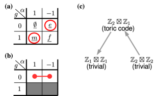
Figure 6: (a) Anyon table for the toric code. $\underline{e}$ and $\underline{m}$ are self-bosons and can condense. (b) Condensation of $\underline{e}$ results in confinement of particles ${\llbracket 1;*\rrbracket}$ (gray) and thus yields a trivial model. (c) Condensation scheme for the Toric Code. The diagram lists the preserved symmetry $\bm{H}$ and the corresponding phases. Note that the two trivial phases correspond to condensing either $\underline{e}$ (left) or $\underline{m}$ (right).

Let us start by considering the Toric Code model $\mathbb{D}(\mathbb{Z}_{2})$. It has four particles: The vacuum $\underline{\emptyset}={\llbracket 0;1\rrbracket}$, the magnetic particle $\underline{m}={\llbracket 1;1\rrbracket}$, the electric particle $\underline{e}={\llbracket 0;-1\rrbracket}$, and the fermion $\underline{f}\equiv\underline{e}\times\underline{m}={\llbracket 1;-1\rrbracket}$; they can be visualized in a two-dimensional grid with $g$ and $\alpha$ as row and column labels, respectively, Fig. 6a. $\underline{e}$ and $\underline{m}$ (marked red) have bosonic self-statistics $\alpha^{g}$ and can therefore condense. Fig. 6b illustrates the condensation of the $\underline{e}$ particle: $\underline{e}$ is identified with the vacuum (indicated by connected dots), and since both $\underline{m}$ and $\underline{f}$ have non-trivial mutual statistics $\alpha^{h}\beta^{g}$ with $\underline{e}$ (as $\alpha=-1$, $g=0$ for $\underline{e}$ and $h=1$ for $\underline{m}$, $\underline{f}$), they become confined (indicated by grayed out boxes).

Let us now study the condensation in terms of the symmetry of the transfer operator. We have $\bm{G}=\mathbb{Z}_{2}\times\mathbb{Z}_{2}$. The possible symmetry breaking patterns $\bm{H}=K\boxtimes L$ are given by $\bm{H}=\mathbb{Z}_{2}\boxtimes\mathbb{Z}_{2}$, $\bm{H}=\mathbb{Z}_{2}\boxtimes\mathbb{Z}_{1}$, and $\bm{H}=\mathbb{Z}_{1}\boxtimes\mathbb{Z}_{1}$, respectively. This is shown in Fig. 6c, where the horizontal layers are arranged according to their “ket-bra symmetry breaking gap” $|K|/|L|$ corresponding to the number of anyons in the model, and the arrows point in the direction of decreased symmetry.

Let us now consider the three possibilities case by case.

1. $\bm{H}=\mathbb{Z}_{2}\boxtimes\mathbb{Z}_{1}$: This is the topological case. On the one hand, we have following Cond. 3 that $\langle S_{\llbracket g;\alpha\rrbracket}\otimes\bar{S}_{\llbracket g;\alpha\rrbracket}\rangle\neq 0$ for all $g$ and $\alpha$, since $(g,g)\in\bm{H}$ and the restriction of $(\alpha,\alpha)$ to $\bm{H}$ is $(\alpha,\alpha)((h,h))=\alpha(h)\bar{\alpha}(h)=1=\nu_{(h,h)}$ [as $\mathrm{H}^{2}(\bm{H},\mathrm{U}(1))$ is trivial]; this is, all particles ${\llbracket g;\alpha\rrbracket}$ are unconfined. On the other hand, $\langle S_{\llbracket g;\alpha\rrbracket}\otimes\bar{S}_{\llbracket g^{\prime};\alpha^{\prime}\rrbracket}\rangle=0$ whenever either $g\neq g^{\prime}$ [as $(g,g^{\prime})\notin\bm{H}$] or $\alpha\neq\alpha^{\prime}$ [as then $(\alpha,\alpha^{\prime})((h,h))\not\equiv 1$]; this is, no particles are condensed.

2. $\bm{H}=\mathbb{Z}_{1}\boxtimes\mathbb{Z}_{1}$: This is the trivial phase in which $\underline{e}={\llbracket 0;-1\rrbracket}$ is condensed (and thus $\underline{m}={\llbracket 1;1\rrbracket}$ is confined). Firstly, since all symmetries are broken, $\langle S_{\llbracket g;\alpha\rrbracket}\otimes\bar{S}_{\llbracket g^{\prime};\alpha^{\prime}\rrbracket}\rangle=0$ whenever $g\neq 0$ or $g^{\prime}\neq 0$, which implies that $\underline{m}$ and $\underline{f}=\underline{e}\times\underline{m}={\llbracket 1;-1\rrbracket}$ are confined. On the other hand, $\langle S_{\llbracket 0;\alpha\rrbracket}\otimes\bar{S}_{\llbracket 0;\alpha^{\prime}\rrbracket}\rangle\neq 0$, since $(0,0)\in\bm{H}$ and $(\alpha,\alpha^{\prime})$ restricted to $\bm{H}$ is trivially the identity, and thus equals $\nu_{(0,0)}$.

3. $\bm{H}=\mathbb{Z}_{2}\boxtimes\mathbb{Z}_{2}$: This is another trivial phase, in which $\underline{m}={\llbracket 1;1\rrbracket}$ is condensed and $\underline{e}={\llbracket 0;-1\rrbracket}$ is confined. Firstly, note that while $\mathrm{H}^{2}(\mathbb{Z}_{2}\boxtimes\mathbb{Z}_{2},\mathrm{U}(1))=\mathbb{Z}_{2}$, we have that $qt=q=2$ and $\mathrm{gcd}(t,q)=1$, i.e., only the trivial cocycle is allowed due to positivity. We have that $\langle S_{\llbracket g;1\rrbracket}\otimes\bar{S}_{\llbracket g^{\prime};1\rrbracket}\rangle\neq 0$ since $(g,g^{\prime})\in\bm{H}$ and $(1,1)=\nu_{(g,g^{\prime})}$, implying that $\underline{m}$ is condensed. On the other hand, $\langle S_{\llbracket g;\alpha\rrbracket}\otimes\bar{S}_{\llbracket g^{\prime};\alpha^{\prime}\rrbracket}\rangle=0$ whenever $\alpha\neq 1$ or $\alpha^{\prime}\neq 1$, since $(\alpha,\alpha^{\prime})((g,g^{\prime}))=\alpha(g)\overline{\alpha^{\prime}}(g^{\prime})\not\equiv 1$ for some $(g,g^{\prime})\in\bm{H}$, i.e., $\underline{e}$ and $\underline{f}$ are confined.

V.2 Condensation of $D(\mathbb{Z}_{4})$

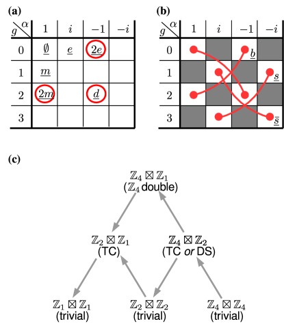
Figure 7: (a) Anyon table for the $D(\mathbb{Z}_{4})$ quantum double model. The first row, first column, and the dyon $\underline{d}$ have bosonic self-statistics and can be condensed. (b) Effective anyon model obtained by condensing $\underline{d}$: The gray anyons become confined, while the remaining ones become identified as indicated. The resulting anyon theory is a doubled semion model with semions $\underline{s}$ and $\underline{\bar{s}}$ with self-statistics $i$. (c) Full condensation scheme for $D(\mathbb{Z}_{4})$. The diagram lists the preserved symmetry $\bm{H}$ and the corresponding phase (TC=toric code, DS=double semion). The case $\bm{H}=\mathbb{Z}_{4}\boxtimes\mathbb{Z}_{2}$ can describe two different topogical phases (TC and DS), depending on the SPT phase of the fixed point.

Let us now turn to our second example, the double $D(\mathbb{Z}_{4})$. The anyon table is given in Fig. 7a; here, we find three bosons (marked red), namely $\underline{2e}$, $\underline{2m}$, and the dyon $\underline{d}=\underline{2e}\times\underline{2m}$. It is straighforward to work out the particle tables obtained by condensation: While condensing $\underline{2e}$ or $\underline{2m}$ leads to two inequivalent toric codes, condensing $\underline{d}$ – as shown in Fig. 7b – leads to the so-called double semion model, with particles $\underline{s}$ and $\underline{\bar{s}}$, which have (anti-)semionic self-statistics $g^{\alpha}=\pm i$, and which fuse with themselves to the vacuum and with each other to the non-trivial boson $\underline{b}={\llbracket 0;-1\rrbracket}\equiv{\llbracket 2;1\rrbracket}$. The double semion model is not a regular double model but can be obtained by twisting $D(\mathbb{Z}_{2})$ with a non-trivial $3$-cocycle of $\mathbb{Z}_{2}$, and is thus the simplest example of a twisted model obtained by condensing a regular double.

Let us now study the possible symmetry breaking pattern $\bm{H}$ of $D(\mathbb{Z}_{4})$, shown in Fig. 7c. We find six possibilities.

1. $\bm{H}=\mathbb{Z}_{4}\boxtimes\mathbb{Z}_{1}$. This is the $D(\mathbb{Z}_{4})$ phase; the discussion is analogous to the case 1 for the Toric Code in Sec. V.1 above.

2. $\bm{H}=\mathbb{Z}_{2}\boxtimes\mathbb{Z}_{1}$. This is a toric code phase in which the $\underline{2e}$ particle has been condensed. We have that $\langle S_{\llbracket g;\alpha\rrbracket}\otimes\bar{S}_{\llbracket g^{\prime};\alpha^{\prime}\rrbracket}\rangle=0$ unless $(g,g^{\prime})\in\bm{H}$, i.e., $g=g^{\prime}=0$ or $g=g^{\prime}=2$, which implies that ${\llbracket 1;*\rrbracket}$ and ${\llbracket 3;*\rrbracket}$ are all confined, and ${\llbracket 2;*\rrbracket}$ is uncondensed. On the other hand, $\langle S_{\llbracket g;\alpha\rrbracket}\otimes\bar{S}_{\llbracket g;\alpha^{\prime}\rrbracket}\rangle\neq 0$ iff $\alpha(g)\overline{\alpha^{\prime}}(g)=1$ (as there is only a trivial cocycle), and thus ${\llbracket 1;-1\rrbracket}$ is condensed, and ${\llbracket 0;i\rrbracket}\equiv{\llbracket 0;-i\rrbracket}$ and ${\llbracket 2;1\rrbracket}\equiv{\llbracket 2;-1\rrbracket}$ form the electric and magnetic particle of the Toric Code, respectively.

3. $\bm{H}=\mathbb{Z}_{4}\boxtimes\mathbb{Z}_{2}$. This is the first case with non-trivial $\mathrm{H}^{2}(\bm{H},\mathrm{U}(1))=\mathbb{Z}_{2}$, and thus exhibits two distinct condensed phases with identical symmetry breaking pattern.
   The phase with trivial cocycle corresponds to a Toric Code phase in which the $\underline{2m}$ particle has been condensed. First, $\langle S_{\llbracket g;\alpha\rrbracket}\otimes\bar{S}_{\llbracket g^{\prime};\alpha^{\prime}\rrbracket}\rangle=0$ whenever $\alpha^{h}\overline{\alpha^{\prime}}{}^{h^{\prime}}\not\equiv 1$ for some $(h,h^{\prime})\in\bm{H}$, i.e. unless $\alpha=\alpha^{\prime}=\pm 1$, and thus ${\llbracket*;\pm i\rrbracket}$ are confined, while ${\llbracket*;-1\rrbracket}$ is not condensed. On the other hand, $\langle S_{\llbracket g;\pm 1\rrbracket}\otimes\bar{S}_{\llbracket g^{\prime};\pm 1\rrbracket}\rangle\neq 0$ iff $(g,g^{\prime})\in\bm{H}$: Thus, ${\llbracket 2;1\rrbracket}$ condenses, and ${\llbracket 1;1\rrbracket}\equiv{\llbracket 3;1\rrbracket}$ and ${\llbracket 0;-1\rrbracket}\equiv{\llbracket 2;-1\rrbracket}$ form the new magnetic and electric particles, respectively.

   Let us now turn towards the phase with non-trivial cocycle. As we will see, it corresponds to a double semion model with the condensation pattern indicated in Fig. 7. It is straightforward to check that for the non-trivial cocycle of $\mathrm{H}^{2}(\bm{H},\mathrm{U}(1))=\mathbb{Z}_{2}$, $\nu_{(g,g^{\prime})}((h,h^{\prime}))=i^{gh}(-i)^{g^{\prime}h^{\prime}}$ (e.g., by checking it on the generators). Then, $\langle S_{\llbracket g;\alpha\rrbracket}\otimes\bar{S}_{\llbracket g^{\prime};\alpha^{\prime}\rrbracket}\rangle=0$ whenever $\alpha^{h}\overline{\alpha^{\prime}}{}^{h^{\prime}}\not\equiv\nu_{(g,g^{\prime})}((h,h^{\prime}))$ for some $(h,h^{\prime})\in\bm{H}$, i.e. unless $\alpha=\pm i^{g}$ and $\alpha^{\prime}=\pm i^{g^{\prime}}$ (with the identical choice of $\pm$). This implies that all ${\llbracket g;\pm i^{g+1}\rrbracket}$ are confined, and only anyons ${\llbracket g;i^{g}\rrbracket}$ can condense. Since $\langle S_{\llbracket g;\alpha\rrbracket}\otimes\bar{S}_{\llbracket 0;1\rrbracket}\rangle\neq 0$ in addition requires $(g,0)\in\bm{H}$, we find that it is ${\llbracket 2;-1\rrbracket}$ which condenses.

4. $\bm{H}=\mathbb{Z}_{1}\boxtimes\mathbb{Z}_{1}$. This is a trivial phase where all $\underline{e}$ particles have been condensed; it is fully analogous to case 2 for the Toric Code in Sec. V.1.

5. $\bm{H}=\mathbb{Z}_{2}\boxtimes\mathbb{Z}_{2}$. This is a trivial phase where $\underline{2e}$ and $\underline{2m}$ have been condensed. We have that $\langle S_{\llbracket g;\alpha\rrbracket}\otimes\bar{S}_{\llbracket g^{\prime};\alpha^{\prime}\rrbracket}\rangle=0$ unless $g,g^{\prime}\in\{0,2\}$, i.e., ${\llbracket 1;*\rrbracket}$ and ${\llbracket 3;*\rrbracket}$ have been confined. It is also zero unless $\alpha^{g}\overline{\alpha^{\prime}}{}^{g^{\prime}}=1$ for all $g,g^{\prime}\in\{0,2\}$ (there is only the trivial cocycle), and thus, ${\llbracket*;\pm i\rrbracket}$ is confined as well. For all remaining cases, $\langle S_{\llbracket g;\alpha\rrbracket}\otimes\bar{S}_{\llbracket g^{\prime};\alpha^{\prime}\rrbracket}\rangle\neq 0$, and thus, all other particles are condensed.

6. $\bm{H}=\mathbb{Z}_{4}\boxtimes\mathbb{Z}_{4}$. This is a trivial phase where all $\underline{m}$ particles have been condensed; it is fully analogous to case 3 for the Toric Code in Sec. V.1. Note that there is again only the trivial cocycle.

V.3 Numerical study

In the following, we provide numerical results on different topological phases which can be obtained through condensation from a $D(\mathbb{Z}_{4})$ double model, and the transitions between them. To this end, we have constructed a three-parameter family interpolating between different fixed point models, including the $D(\mathbb{Z}_{4})$ phase, both Toric Code phases, the double semion phase, and a trivial phase. Here, we will limit ourselves to a brief overview of the results; an in-depth discussion of the specific wavefunction family considered as well as the numerical methods used, together with additional results, will be presented elsewhere iqbal:preparation .

Let us start by introducing the family of tensors used:

$$A\left(\theta_{\mathrm{DS}},\theta_{\mathrm{TC},\mathbb{Z}_{2}},\theta_{\mathrm{TC}}\right)=\vbox{\hbox{\includegraphics[width=43.36464pt]{figs/z4phdiag_1}}}\ .$$ (25)

Here, the four outside legs correspond to the virtual indices, while the four inside legs are the physical indices. The rings (and the green dots) describe MPOs all of which mutually commute:

• The outermost black ring is the MPO of the $D(\mathbb{Z}_{4})$ quantum double, $\sum_{g}U_{g}^{\otimes 4}$, $U_{g}=X^{g}$, with $X$ the generator of the regular representation of $\mathbb{Z}_{4}$.

• The red ring describes a deformation towards the MPO projector for the $\mathbb{Z}_{4}\boxtimes\mathbb{Z}_{2}$ double semion model, where

  $$\vbox{\hbox{\includegraphics[width=26.01613pt]{figs/ds_protensor_2}}}=(X^{2})^{i}(Z^{2})^{i+j},\quad i,j=0,1\ ,$$

  with $Z$ the generator of the diagonal representation of $\mathbb{Z}_{4}$, and $\vbox{\hbox{\includegraphics[width=26.01613pt]{figs/z4qd_ds_1}}}=\mathrm{diag}(\cosh\tfrac{\theta_{\mathrm{DS}}}{2},\sinh\tfrac{\theta_{\mathrm{DS}}}{2})$. For $\theta_{\mathrm{DS}}=\infty$ (and $\theta_{\mathrm{TC},\mathbb{Z}_{2}}=\theta_{\mathrm{TC}}=0$), this gives the double semion MPO, while for $\theta_{\mathrm{DS}}=0$, it acts trivially.

• The blue ring describes a deformation towards the $\bm{H}=\mathbb{Z}_{2}\boxtimes\mathbb{Z}_{1}$ Toric Code, where

  $$\raisebox{-11.99998pt}{\includegraphics[width=30.00005pt]{figs/z4qd_ds_3_0}}=\delta_{ij}\exp((-1)^{i}\theta_{\mathrm{TC},\mathbb{Z}_{2}}Z^{2}),\ i,j=0,1\ .$$

  For $\theta_{\mathrm{TC},\mathbb{Z}_{2}}=\infty$, this projects the $D(\mathbb{Z}_{4})$ MPO onto a $\mathbb{Z}_{2}$ subgroup and thus yields the Toric Code, while for $\theta_{\mathrm{TC},\mathbb{Z}_{2}}=0$, it acts trivially.

• Green circles $\vbox{\hbox{\includegraphics[width=30.00005pt]{figs/z4qd_ds_2}}}=\exp\left(\theta_{TC}X^{2}\right)$ describe a deformation towards a $\bm{H}=\mathbb{Z}_{4}\boxtimes\mathbb{Z}_{2}$ Toric Code phase: For $\theta_{\mathrm{TC}}=\infty$, this enhances the symmetry of the $D(\mathbb{Z}_{4})$ MPO to $\bm{H}=\mathbb{Z}_{4}\boxtimes Z_{2}$, while for $\theta_{\mathrm{TC}}=0$, it once again acts trivially.

The two Toric Code constructions correspond to the two ways of embedding a “normal” $\mathbb{Z}_{2}\boxtimes\mathbb{Z}_{1}\subset\mathbb{Z}_{2}\times\mathbb{Z}_{2}$ Toric Code into a $\mathbb{Z}_{4}\times\mathbb{Z}_{4}$ symmetry described in Sec. IV.2.2. Note that since all projectors commute with each other, their order does not matter.

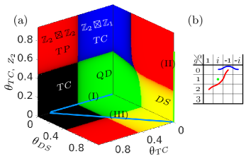
Figure 8: Three surfaces in the $3$-parameter phase diagram described in Sec. V.3. The RGB values of each point give the expectation value of the string order parameters indicated in panel (b), cf. also Fig. 9: Red $=\langle S_{\llbracket 2;1\rrbracket}\otimes\bar{S}_{\llbracket 0;-1\rrbracket}\rangle$, Green $=\langle S_{\llbracket 1;i\rrbracket}\otimes\bar{S}_{\llbracket 1;i\rrbracket}\rangle$, Blue $=\langle S_{\llbracket 0;i\rrbracket}\otimes\bar{S}_{\llbracket 0;-i\rrbracket}\rangle$, the three of which jointly allow to discriminate all the phases observed. QD, TC, DS, and TP denote the $D(\mathbb{Z}_{4})$ double model, toric code, double semion, and trivial phase, respectively. Note that the phase diagram exhibits two distinct toric code phases ($\mathbb{Z}_{2}\boxtimes\mathbb{Z}_{1}$, blue, and $\mathbb{Z}_{4}\boxtimes\mathbb{Z}_{2}$, black), while all three trivial phases have symmetry $\mathbb{Z}_{2}\boxtimes\mathbb{Z}_{2}$.

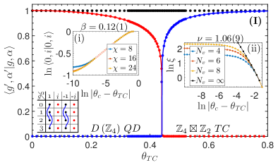
Figure 9: String order parameters for condensation and deconfinement for the interpolation (I) in Fig. 8a, describing a $D(\mathbb{Z}_{4})$ to Toric Code transition, obtained by approximating the fixed point of $\mathbb{T}$ with an iMPS of bond dimension $\chi=24$. The type of string order parameters is encoded by the color, as indicated in the anyon table in the lower left corner: Dots correspond to the deconfinement parameter $\langle S_{\llbracket g;\alpha\rrbracket}\otimes\bar{S}_{\llbracket g;\alpha\rrbracket}\rangle\equiv\langle g,\alpha|g,\alpha\rangle$, while lines correspond to condensate fractions $\langle S_{\llbracket g;\alpha\rrbracket}\otimes\bar{S}_{\llbracket g^{\prime};\alpha^{\prime}\rrbracket}\rangle\equiv\langle g,\alpha|g^{\prime},\alpha^{\prime}\rangle$ for the pairs they connect; order parameters with the same color are (numerically) identical. Specifically, the blue line gives the condensate fraction of the $\underline{2m}={\llbracket 2;1\rrbracket}$ magnetic particle, and the red line measures the deconfinement of the $\underline{e}={\llbracket 0;i\rrbracket}$ particle, which becomes confined if $\underline{2m}$ condenses. The solid line is the analytical result from the mapping to the 2D Ising model, showing excellent agreement. The upper left inset (i) shows the scaling of the deconfinement parameter $\langle S_{\llbracket 0;i\rrbracket}\otimes\bar{S}_{\llbracket 0;i\rrbracket}\rangle$ in the vicinity of critical point, with critical exponent $\beta=0.12(1)$. The right insets (ii) give the correlation length around the critical point and the corresponding critical exponent $\nu=1.06(9)$, extracted from exact diagonalization of the transfer operator on cylinders of diameter $N_{v}$; the extrapolation $N_{v}=\infty$ has been obtained by fitting with $a\exp\left(-bN_{v}\right)+C_{\infty}$. We find that the critical exponents are the same on both sides of the phase transition.

We have studied the phase diagram of this family using infinite Matrix Product States (iMPS) to approximate the fixed point of the transfer operator, by iteratively applying the transfer operator and truncating the bond dimension to some given $\chi$, keeping translational symmetry. From the resulting fixed point iMPS, we can then [using Eq. (15)] immediately compute the order parameters for condensation, $\langle S_{\llbracket g;\alpha\rrbracket}\otimes\bar{S}_{\llbracket 0;1\rrbracket}\rangle$, and deconfinement, $\langle S_{\llbracket g;\alpha\rrbracket}\otimes\bar{S}_{\llbracket g;\alpha\rrbracket}\rangle$, respectively, allowing us to distinguish the different topological phases and map out the phase diagram. The condensation and deconfinement order parameters also allow us to study the nature of the phase transitions. Notably, this gives us non-zero order parameters, and thus critical exponents $\beta$, for both sides of a condensation-driven phase transition: in the uncondensed phase, the deconfinement order parameter is non-zero, while in the condensed phase, the condensate fraction is non-zero. Note that we use the string operator corresponding to excitations in the fixed point wavefunction to measure the order parameter throughout the phase diagram; this is in exact analogy to the use of order parameters in conventional phase transitions. In addition to that, we can further characterize the phase transition by looking at the scaling of the correlation length $\xi$, which we can extract either from the fixed point iMPS, or from the finite-size transfer operator and a finite size scaling (note though that this length does need not be equal to the physical correlation length, as it includes e.g. certain anyon-anyon correlation functions).

In order to understand the structure of our three-parameter family, Eq. (25), we have computed the different condensation and deconfinement order parameters along the three hyperplanes for which one $\theta_{\bullet}=0$; the resulting phase diagram is shown in Fig. 8. We find that the system exhibits all phases encoded by the three MPOs in Eq. (25), as well as a trivial phase with $\bm{H}=\mathbb{Z}_{2}\boxtimes\mathbb{Z}_{2}$, which can be understood analytically in the limit where two of the $\theta_{\bullet}$ are taken to infinity. As expected, the family thus exhibits phase transitions related to the condensation of anyons from $D(\mathbb{Z}_{4})$ to Toric Code and Double Semion, and from either to the trivial phase; more notably, though, the family also exhibits direct phase transitions between the Toric Code and the Double Semion model, which are not related by anyon condensation.

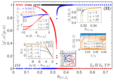
Figure 10: Phase transition between double semion model ($\mathbb{Z}_{4}\boxtimes Z_{2}$ symmetry) and trivial phase ($\mathbb{Z}_{2}\boxtimes\mathbb{Z}_{2}$ symmetry) along line (II) in Fig. 8. The plot shows the deconfinement/condensate order parameters (color coded as indicated by the dots/lines in the anyon table in the inset) vs. the interpolation parameter $\theta_{\mathrm{TC},\mathbb{Z}_{2}}$; see Fig. 9 for details. Insets (i) and (ii) are the same as in Fig. 9, giving fits for the critical exponents $\beta_{\pm}$ and $\nu$, respectively. Inset (iii) shows the behavior condensate fraction $\langle S_{\llbracket 2;1\rrbracket}\otimes\bar{S}_{\llbracket 0;1\rrbracket}\rangle\equiv\langle 2,1|0,1\rangle$ (blue in the main plot) close to the phase transition for different iMPS bond dimensions $\chi$, demonstrating convergence to a smooth (albeit steep) curve. In inset (iv), the same data is plotted against $1/\chi$ for different $\theta_{TC,\mathbb{Z}_{2}}$, reconfirming the second-order nature of the transition [compare with inset (ii) of Fig. 11b!], and allowing us to accurately localize the phase transition.

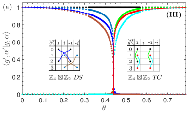
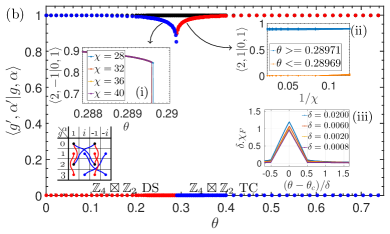
Figure 11: Condensation and deconfinement order parameters for two phase transitions between the Double Semion model (left) and the $\mathbb{Z}_{4}\boxtimes\mathbb{Z}_{2}$ Toric Code (right), corresponding to an SPT transition at the boundary, cf. Fig. 9. (a) Interpolation along the line (III) in Fig. 8a, cf. inset for the color coding. The order parameters for condensation of the dyon $\underline{d}={\llbracket 2;-1\rrbracket}$ (blue) and deconfinement of the magnon $\underline{m}={\llbracket 1;1\rrbracket}$ (red) can be mapped to the magnetization of the 2D Ising model (solid lines). (b) Interpolation obtained by interpolating the per-site transfer operator, cf. text, showing clear signs of a first-order phase transition. This is further supported by the analysis in the insets: (i) gives the behavior of the condensate fraction of the dyon $\underline{d}={\llbracket 2;-1\rrbracket}$ (blue) in the vicinity of the phase transition for different $\chi$, showing convergence to a discontinuous curve. (ii) gives the same data as a function of $1/\chi$ for different $\theta$, and we observe a sharp change of the behavior at $\theta\approx 0.28970$. [(i) and (ii) should be contrasted with insets (iii) and (iv) of Fig. 10.] Finally, inset (iii) gives the fidelity susceptibility $\chi_{F}$, measuring the rate of change of the normalized wave function $|\hat{\psi}(\theta)\rangle$ with $\theta$, $|\langle\hat{\psi}(\theta)|\hat{\psi}(\theta+\mathrm{d}\theta)\rangle|=1-\tfrac{1}{2}\chi_{F}N^{2}(\mathrm{d}\theta)^{2}$, for different step sizes $\mathrm{d}\theta=\delta\rightarrow 0$, which approaches a delta peak as expected for a first-order transition zanardi:overlap-curvature ; gu:fidelity-phasetransitions .

We have studied a number of these phase transitions in more detail; in the following, we illustrate our findings through a few examples, and refer the reader for a more detailed analysis to Ref. iqbal:preparation . First, we have studied the phase transitions in the $\theta_{\mathrm{TC},\mathbb{Z}_{2}}=0$ plane. Fig. 9 shows the order parameters along line (I) in Fig. 8, which describes a $D(\mathbb{Z}_{4})$ to Toric Code transition. Since we have an analytical mapping to the 2D Ising model for this line, it can serve as a benchmark, and we find indeed very good agreement with the analytic predictions. Further study suggests the existence of an analytical mapping for the entire $\theta_{\mathrm{TC},\mathbb{Z}_{2}}=0$ plane; for the $\theta_{\mathrm{DS}}=0$ plane, the critical exponents still match those of the 2D Ising model, though the existence of an exact mapping is unclear. On the other hand, the transitions in the $\theta_{\mathrm{TC}}=0$ plane seem to belong to a different universality class. As an example, Fig. 10 shows the transition along the line (II) in Fig. 8, for which we find critical exponents $\nu=1.05(7)$ for the correlations in the fixed point of the transfer operator, and $\beta_{+}=0.04(1)$ and $\beta_{-}=0.23(4)$ for the anyon condensation and deconfinement order parameters, respectively; notably, the critical exponent $\beta$ is different on the two sides of the transition. We observe that the critical exponents $\beta_{\pm}$ change continously as we move along the transition line in the $\theta_{\mathrm{DS}}=1$ plane towards the $\theta_{\mathrm{TC},\mathbb{Z}_{2}}$ plane, ultimately reaching $\beta_{\pm}=1/8$; a detailed discussion will be given elsewhere iqbal:preparation .

Finally, let us turn towards the direct Toric Code – Double Semion transition, previously only studied with exact diagonalization and on quasi-1D systems morampudi:z2-phase-transition , whose nature is yet to be resolved. As one would assume that interactions generally give rise to condensation of excitations, one expects that an interpolation between the two models would typically drive the Toric Code through some condensation transition, either into a trivial or a more complex phase [such as the $D(\mathbb{Z}_{4})$ model], and from there through another condensation-driven transition to the Double Semion model, and a direct transition would at least require some fine-tuning of interactions.

We can identify one such fine-tuned transition between the ($\bm{H}=\mathbb{Z}_{4}\boxtimes\mathbb{Z}_{2}$) Toric Code and Double Semion phase in our phase diagram in the $\theta_{\mathrm{TC},\mathbb{Z}_{2}}=0$ plane at $\left(\theta_{\mathrm{DS}}^{c},\theta^{c}_{\mathrm{TC}}\right)=\left(\tfrac{1}{2}\ln(1+\sqrt{2}),\ \tfrac{1}{2}\ln(1+\sqrt{2})\right)$; this is a multi-critical point adjacent to all four phases which goes away as one perturbs away from $\theta_{\mathrm{TC},\mathbb{Z}_{2}}=0$, separating the Toric Code from the Double Semion phase. Fig. 11a shows the transition through this point along line (III) in Fig. 8, and we find that it is a second order phase transition, driven by two “counterpropagating” condensation and de-condensation transitions, thus preserving the total number of anyons; like all transitions in that plane, it is again in the 2D Ising universality class. Note however that this is a phase transition between two phases with an identical $\bm{H}=\mathbb{Z}_{4}\boxtimes\mathbb{Z}_{2}$ symmetry at the boundary, and therefore corresponds to an SPT phase transition at the boundary in the absence of symmetry breaking, and can therefore only be detected by string order parameters rather than conventional local order parameters. Note however that it has been shown that in certain cases string order parameters can be mapped to local order parameters through a duality mapping duivenvoorden:stringorder-symbreaking .

As it turns out, there is another way of obtaining a direct phase transition between the $\bm{H}=\mathbb{Z}_{4}\boxtimes\mathbb{Z}_{2}$ Toric Code and Double Semion phase, namely by interpolating between the on-site transfer operators $A^{\dagger}A$ of the two fixed point models, rather than the tensors $A$ themselves. Since such an interpolation $\mathbb{E}(\theta)=\theta A_{0}^{\dagger}A_{0}+(1-\theta)A_{1}^{\dagger}A_{1}$ yields a positive semidefinite $\mathbb{E}(\theta)\geq 0$, we can construct a continuous path $A(\theta)$ of PEPS tensors by decomposing $\mathbb{E}(\theta)=A(\theta)^{\dagger}A(\theta)$. This interpolation yields again a direct transition between the two phases, and a thorough analysis of the order parameters, shown in Fig. 11b, gives compelling evidence that the phase transition is first order. Thus, in order to understand the nature of a generic Toric Code – Double Semion phase transition (given it can even be realized in a robust way) requires further study. In this context, it is an interesting question whether imposing specific symmetries on the system allows one to generically obtain a direct transition between these two phases, rather than requiring fine-tuning of the interactions.

VI Conclusions and outlook

In this paper, we have studied anyon condensation in Projected Entangled Pair State models, and have derived conditions governing the condensation and confinement of anyons. In order to do so, we have related the behavior of anyons to string order parameters and thus symmetry protected order in the fixed point of the transfer operator, this is, the entanglement spectrum of the system. We have derived four conditions: Two characterize the possible symmetry breaking and SPT phases consistent with positivity of the entanglement spectrum, while the other two related these symmetry breaking and SPT patterns to the condensation and confinement of anyons. Specifically, we found that there are topological phases which cannot be distinguished through their symmetry breaking pattern, but solely through the SPT structure of their entanglement spectrum, and which describe phases not related by anyon condensation. For the case of cyclic groups, this classification allowed to construct all twisted doubles by condensing non-twisted double models.

We have exemplified our discussion with the $\mathbb{Z}_{4}$ quantum double, which can give rise to both Toric Code and Double Semion phases which form an example of phases with identical symmetry breaking pattern but inequivalent SPT order in the entanglement spectrum. We have also provided numerical results for the phase diagram and the phase transitions of the model. To this end, we have used that the concepts developed in this paper allow us to measure order parameters for condensation and deconfinement and thus extract critical exponents for the order parameter. In particular, we found that this model can realize direct phase transitions between the Toric Code and Doubled Semion models which are not related by anyon condensation, and for which we found both first and second order transitions.

A natural question is the interpretation of symmetry broken and SPT phases in the fixed point of the transfer operator in terms of physical properties of the entanglement spectrum and/or edge physics yang:peps-edgetheories : Symmetries $U_{g}\rho U_{g}^{\dagger}=\rho$ imply that the entanglement spectrum $\rho$ is block-diagonal, i.e., it originates from a symmetric Hamiltonian. An additional single-layer symmetry $U_{g}\rho=\rho$ implies that the density operator must live in the trivial irrep sector, while a broken symmetry and the resulting dependence on distant boundary conditions implies the existence of a non-local anomalous term in the entanglement Hamiltonian which depends on distant boundaries and encodes a topological superselection rule schuch:topo-top . The implications of SPT order on the entanglement spectrum, on the other hand, are much less clear, and it would be very interesting to identify the features of the entanglement spectrum which would allow to distinguish e.g. Toric Code and Doubled Semion order.

It is likely that our results generalize to the case of non-abelian groups, and beyond that to general Matrix Product Operator symmetries bultinck:mpo-anyons . An obstacle is that the one-to-one correspondence between string order parameters and SPTs breaks down pollmann:spt-detection-1d : While it is known that non-abelian SPTs are still characterized by group cohomology, we have used SPT phases to classify the behavior of string order parameters rather than the other way around, and are thus looking for a classification of the behavior of non-abelian string order parameters instead. Let us note, however, that a major simplification might come from the fact that for non-abelian double models, the irrep at the end of a string must be an irrep of its normalizer, so it might well be possible that the problem can be abelianized to an extent which allows to yet again relate it to SPT order. A related question is the generalization of our results to the case of non-hermitian transfer operators, or even PEPS which encode a corresponding global symmetry in a non-trivial way. In that case, string order parameters are evaluated between non-identical left and right fixed points, and the analogy to expectation values in physical states, and thus the correspondence of string order parameters with SPT phases, breaks down; for instance, it is not even clear whether the projective symmetry representation for pairs of left and right fixed points must be equal.

Finally, the maybe most important question, which goes far beyond the scope of this work, is a rigorous justification of our main technical assumption, namely that the structure of the fixed point space of a transfer operator for a PEPS in a gapped phase is well described by Matrix Product Operators. While this is well motivated due to the short-range nature of the correlations in the system, and is well-tested numerically through numerous PEPS simulations using contraction schemes which model the boundary as an MPO, it has withstood rigorous assessment up to now. A better understanding of this question would lead to a number of important insights regarding the structure of gapped phases, the nature of the entanglement spectrum, or the convergence of numerical methods, just to name a few.

Appendix A Construction of explicit endpoints

In this appendix, we provide an explicit construction for all anyons ${\llbracket g;\alpha\rrbracket}$ which are either condensed or deconfined following Condition 3, i.e. $\bm{\alpha}|_{\bm{H}}=\nu_{\bm{g}}$. To this end, we proceed in two steps: First, we generalize the construction of Eq. (17) to obtain $\bm{R}_{\bm{\alpha}}$ which transform as irreps $\bm{\alpha}$ of $\bm{G}$ rather than only $\bm{H}$. Second, we show that for the case of condensation, $\bm{g}=(g,e)$ and $\bm{\alpha}=(\alpha,1)$, and for the case of deconfinement, $\bm{g}=(g,g)$ and $\bm{\alpha}=(\alpha,\alpha)$, these $\bm{R}_{\bm{\alpha}}$ allow to construct actual anyons, i.e., single-layer endpoints, for which $\langle\bm{S}_{\llbracket\bm{g};\bm{\alpha}\rrbracket}\rangle\neq 0$; this is exactly what is also required in Section III.7, where we derive the anyon condensation rules from Conditions 1–4.

A.1 Construction of $\bm{R}_{\bm{\alpha}}$ for irreps of $\bm{G}$

Let $\bm{g}\in\bm{H}$, and $\bm{\alpha}$ an irrep of $\bm{G}$ such that $\bm{\alpha}|_{\bm{H}}=\nu_{\bm{g}}$. The idea of Eq. (17) was to use injectivity of the MPS tensor $M$ to define $\bm{R}_{\bm{\alpha}}$ such that

$$\raisebox{-30.00005pt}{\includegraphics[scale={0.7}]{figs/app1_ralpha_olddef}}\quad.$$

The tensor $M$ describes one symmetry-broken sector (with residual symmetry group $\bm{H}$) only. In order to construct some $\bm{R}_{\bm{\alpha}}$ which transforms as an irrep of $\bm{G}$, we therefore first need to construct an MPS which does not break the symmetry. To this end, choose representants $\bm{f}_{\mathfrak{a}}\in\bm{G}$ of every symmetry-broken sector $\mathfrak{a}\in\bm{G}/\bm{H}$, such that

$$\bm{G}=\bigoplus_{\mathfrak{a}\in\bm{G}/\bm{H}}\bm{f}_{\mathfrak{a}}\bm{H}\ ;$$

by starting from the generators of the quotient group $\bm{G}/\bm{H}$, it is possible to pick $\bm{f}_{\mathfrak{a}}$ such that $\bm{f}_{\mathfrak{ab}}=\bm{f}_{\mathfrak{a}}\bm{f}_{\mathfrak{b}}$. Now define

and $\mathcal{M}^{i}=\bigoplus_{\mathfrak{a}}M^{i}_{\mathfrak{a}}$; clearly, $\mathcal{M}^{i}$ is block-injective (i.e., injective on the space of block-diagonal matrices). Given $\bm{k}\in\bm{G}$, there is a unique decomposition $\bm{k}=\bm{f}_{\mathfrak{a}}\bm{h}$, $\bm{h}\in\bm{H}$, and thus

$$\raisebox{-26.00009pt}{\includegraphics[scale={0.7}]{figs/app1_Ug_virt_action}}\quad;$$

this is, the virtual action of $\bm{U}_{\bm{k}}$ is

$$\mathcal{V}_{\bm{k}}:=\left(\bigoplus\bm{V}_{\bm{h}}\right)\Pi_{\mathfrak{a}}\ ,$$

where $\Pi_{\mathfrak{a}}$ permutes the blocks by virtue of $\mathfrak{b}\mapsto\mathfrak{a}^{-1}\mathfrak{b}$; note that $\mathcal{V}_{\bm{k}}$ forms a projective representation of $\bm{G}$ (the trivial induced projective representation induced by $\bm{V}_{\bm{h}}$). Now define

$$\mathcal{W}:=\bigoplus_{\mathfrak{b}}{\bm{\alpha}(\bm{f}_{\mathfrak{b}})}\bm{V}_{\bm{g}}\ ,$$

and choose $\bm{R}_{\bm{\alpha}}$ such that

– this is always possible since $\mathcal{W}$ is block-diagonal and $\mathcal{M}$ is block-injective. (We use a thick line to indicate the larger “direct sum” virtual space.) We now have that

$$\mathcal{V}_{\bm{k}}\mathcal{W}\mathcal{V}_{\bm{k}}^{\dagger} =\left[\Big{(}\bigoplus\bm{V}_{\bm{h}}\Big{)}\Pi_{\mathfrak{a}}\right]\Big{[}\bigoplus_{\mathfrak{b}}{\bm{\alpha}(\bm{f}_{\mathfrak{b}})}\bm{V}_{\bm{g}}\Big{]}\left[\Pi_{\mathfrak{a}}^{\dagger}\Big{(}\bigoplus\bm{V}^{\dagger}_{\bm{h}}\Big{)}\right]$$

$$=\left[\Big{(}\bigoplus\bm{V}_{\bm{h}}\Big{)}\right]\Big{[}\bigoplus_{\mathfrak{b}^{\prime}}{\bm{\alpha}(\bm{f}_{\mathfrak{a}\mathfrak{b}^{\prime}})}\bm{V}_{\bm{g}}\Big{]}\left[\Big{(}\bigoplus\bm{V}_{\bm{h}}^{\dagger}\Big{)}\right]$$

$$=\nu_{\bm{g}}(\bm{h})\Big{[}\bigoplus_{\mathfrak{b}^{\prime}}{\bm{\alpha}(\bm{f}_{\mathfrak{a}\mathfrak{b}^{\prime}})}\bm{V}_{\bm{g}}\Big{]}=\nu_{\bm{g}}(\bm{h})\bm{\alpha}(\bm{f}_{\mathfrak{a}})\mathcal{W}$$

$$=\bm{\alpha}(\bm{k})\mathcal{W}\ ,$$

where we have used $\nu_{\bm{g}}(\bm{h})=\bm{\alpha}(\bm{h})$. It immediately follows that

i.e., $\bm{R}_{\bm{\alpha}}$ indeed transforms as the irrep $\bm{\alpha}$ of $\bm{G}$.

A.2 Explicit construction of condensed anyons

Let us now show that we can explicitly construct condensed anyons ${\llbracket g;\alpha\rrbracket}$: Given a $\bm{R}_{(\alpha,1)}$ for which $\langle\bm{S}_{\llbracket{(g,e)};{(\alpha,1)}\rrbracket}\rangle\neq 0$, we show how to construct a single-layer anyon (i.e., an endpoint to a string of $g$’s transforming like $\alpha$) with non-zero expectation value $\langle S_{\llbracket g;\alpha\rrbracket}\otimes\bar{S}_{\llbracket e;1\rrbracket}\rangle\neq 0$, where the endpoint in the bra layer is trivial. To this end, we start by decomposing

$$\bm{R}_{(\alpha,1)}=\sum X^{s}_{\alpha}\otimes\bar{Y}^{s}_{1}\ ,$$

where $X_{\alpha}$ and $Y_{1}$ transform like $\alpha$ and trivially, respectively. Since $R_{(\alpha,1)}$ gives a non-zero expectation value $\langle\bm{S}_{\llbracket{(g,e)};{(\alpha,1)}\rrbracket}\rangle\neq 0$, there must be at least one $s_{0}$ for which this also holds; we thus obtain a separable endpoint $X^{s_{0}}_{\alpha}\otimes\bar{Y}^{s_{0}}_{1}\equiv X_{\alpha}\otimes\bar{Y}_{1}$ with $\langle\bm{S}_{\llbracket{(g,e)};{(\alpha,1)}\rrbracket}\rangle\neq 0$; however, $Y_{1}$ can still be different from the identity. In order to make the endpoint in the bra layer entirely trivial, we use that

since $A$ is $G$-injective (and $C$ is $G$-invariant), and thus,

with the endpoint

for the condensed anyon ${\llbracket g;\alpha\rrbracket}$.

Note that a simple application of Cauchy-Schwarz yields that any condensed anyon is also deconfined.

A.3 Explicit construction of deconfined anyons

Similar to the preceding section, in this scenario we start from some $\bm{R}_{(\alpha,\alpha)}$ s.th. $\langle\bm{S}_{\llbracket{(g,g)};{(\alpha,\alpha)}\rrbracket}\rangle\neq 0$, corresponding to a deconfined anyon ${\llbracket g;\alpha\rrbracket}$, and want to construct identical endpoints $Z_{\alpha}$ for the ket and bra layer such that $\langle S_{\llbracket g;\alpha\rrbracket}\otimes\bar{S}_{\llbracket g;\alpha\rrbracket}\rangle\neq 0$. We again start by decomposing

$$\bm{R}_{(\alpha,\alpha)}=\sum X^{s}_{\alpha}\otimes\bar{Y}^{s}_{\alpha}\ .$$

Let us define the shorthand $\langle X_{\alpha}\otimes Y_{\alpha}\rangle:=\langle S_{\llbracket g;\alpha\rrbracket}\otimes\bar{S}_{\llbracket g;\alpha\rrbracket}\rangle$, where $S\otimes\bar{S}$ has endpoints $X\otimes Y$. Now pick $s_{0}$ such that $\langle X_{\alpha}\otimes\bar{Y}_{\alpha}\rangle\equiv\langle X^{s_{0}}_{\alpha}\otimes\bar{Y}^{s_{0}}_{\alpha}\rangle\neq 0$. If $\langle X_{\alpha}\otimes\bar{X}_{\alpha}\rangle\neq 0$ or $\langle Y_{\alpha}\otimes\bar{Y}_{\alpha}\rangle\neq 0$, we can choose $Z_{\alpha}:=X_{\alpha}$ (or $Z_{\alpha}:=Y_{\alpha}$), and have found the desired non-vanishing identical ket and bra endpoint $\langle Z_{\alpha}\otimes Z_{\alpha}\rangle\neq 0$. Let us now consider the case where both are zero. Let $\phi$ such that $\langle X_{\alpha}\otimes e^{-i\phi}\bar{Y}_{\alpha}\rangle>0$, and define $Z_{\alpha}:=X_{\alpha}+e^{i\phi}Y_{\alpha}$. Then,

$$\langle Z_{\alpha}\otimes\bar{Z}_{\alpha}\rangle =\langle X_{\alpha}\otimes\bar{X}_{\alpha}\rangle+\langle Y_{\alpha}\otimes\bar{Y}_{\alpha}\rangle$$

$$\quad\qquad+\langle X_{\alpha}\otimes e^{-i\phi}\bar{Y}_{\alpha}\rangle+\langle e^{i\phi}Y_{\alpha}\otimes\bar{X}_{\alpha}\rangle$$

$$=2\mathrm{Re}\,\langle X_{\alpha}\otimes e^{-i\phi}\bar{Y}_{\alpha}\rangle>0\ ,$$

thus again yielding identical endpoints $Z_{\alpha}$ for ket and bra with non-vanishing expectation value.

Appendix B Generalization to dressed endpoints

Let us now show that the no-go results of Conditions 1–4 derived in Sec. III equally hold for general endpoints; the explicit construction for any endpoint compatible with all the conditions has already been provided in Appendix A. Let us recall that a general anyon is of the form

$$\raisebox{-22.76228pt}{\includegraphics[scale={0.6}]{figs/app2_gen_anyon}}\ .$$

For deriving the no-go results, we generally need to consider joint ket-bra objects; we thus define

$$\raisebox{-15.6491pt}{\includegraphics[scale={0.7}]{figs/app2_bmAdef}}\mbox{\quad and\quad}\raisebox{-15.6491pt}{\includegraphics[scale={0.7}]{figs/app2_bmRdef}}\ .$$

The generalization of Eq. (10), describing a general string order parameter for a ket and bra anyon pair, evaluated in a pair of fixed points $|\rho_{\bm{c}})$ and $(\rho_{\bm{c}^{\prime}}|$, is thus of the form

$$O_{\bm{c}}^{\bm{c}^{\prime}}:=\raisebox{-36.98866pt}{\includegraphics[scale={0.7}]{figs/app2_sop_pair_mixed}}\quad.$$ (26)

Just as in Sec. III, a central role will be played by the (mixed) transfer operator $\tilde{\mathbb{E}}_{\bm{c}}^{\bm{c}^{\prime}}$; we will therefore analyze its structure in detail in the following.

B.1 Structure of $\tilde{\mathbb{E}}_{\bm{c}}^{\bm{c}^{\prime}}$

The major complication as compared to the discussion in Section III is that for an $M\equiv M^{\bm{c}}$ describing an injective MPS $|\rho)$ which is a fixed point of the transfer operator, the tensor

$$D:=\quad\raisebox{-16.00008pt}{\includegraphics[scale={0.7}]{figs/app2_AM}}$$

describing the MPS obtained after applying $\mathbb{T}$ only needs to be proportional to $|\rho)$, with a possibly size-dependent proportionality constant. This has two consequences perez-garcia:mps-reps ; cirac:mpdo-rgfp : First, $D$ can consists of several diagonal blocks $D_{s,s}$, $s=1,\dots,S$ each of which describes a copy of the original MPS, i.e., $D_{s,s}=\tilde{M}^{i}_{s}$, where each $\tilde{M}^{i}_{s}$ is equal to $M^{i}$ up to a block-dependent gauge transform, $\tilde{M}^{i}_{s}=\gamma_{s}X_{s}M^{i}X_{s}^{-1}$ with some left-invertible $X_{s}$. Second, there can in addition be off-diagonal blocks $D_{s,t}$ coupling blocks $s$ and $t$, which however—up to reordering of blocks—must be upper triangular, i.e., $D_{s,t}\equiv 0$ if $s>t$. This implies that any product $D^{i_{1}}D^{i_{2}}\cdots D^{i_{L}}$ can contain each off-diagonal block $D^{i}_{s,t}$ at most once, and in particular contains only a finite number of off-diagonal blocks. W.l.o.g., we will assume that $D$ is normalized such that the largest $|\gamma_{s}|=1$, with the normalization of the $M^{i}$ as before.

Let us now consider what this implies when taking large powers $\mathbb{(}\tilde{\mathbb{E}}^{\bm{c}^{\prime}}_{\bm{c}})^{K}$, $K\rightarrow\infty$. In that case, there will be large contiguous blocks of the form $F_{s}:=\sum D_{s}^{i,\bm{c}^{\prime}}\otimes\bar{M}^{i,\bm{c}}=\gamma_{s}\sum X_{s}M_{s}^{i,\bm{c}^{\prime}}X_{s}^{-1}\otimes\bar{M}^{i,\bm{c}}$ (specifically, there will be at least one block with length at least $K/S$), which will therefore converge to the fixed point of the corresponding original transfer operator $\mathbb{E}^{\bm{c}^{\prime}}_{\bm{c}}$, up to normalization and a gauge transform. In particular, this implies for $\bm{c}\neq\bm{c}^{\prime}$ that $(\tilde{\mathbb{E}}_{\bm{c}}^{\bm{c}^{\prime}})^{K}$ decays exponentially in $K$. For $\bm{c}=\bm{c}^{\prime}$, pick the largest contiguous block $F_{s}$ within $(\tilde{\mathbb{E}}_{\bm{c}}^{\bm{c}})^{K}$, and notice that it converges to a rank-$1$ projector onto its non-degenerate leading eigenvectors, which therefore transform trivially under the group action. Since $\tilde{\mathbb{E}}_{\bm{c}}^{\bm{c}}$ commutes with the symmetry action, further applications of $\tilde{\mathbb{E}}_{\bm{c}}^{\bm{c}}$ to this rank-$1$ projector do not change the irrep label of the fixed point. (The symmetry actions on the different blocks are related by the corresponding gauge transform $X_{s}$ and label irreducible representations in the same way; note that we only care about the symmetry action on the bond degree of freedom of the MPS to the extent they are related to order parameters, i.e., the symmetry action on the “physical” degrees of freedom.) $(\tilde{\mathbb{E}}^{\bm{c}}_{\bm{c}})^{K}$ will generally be a sum over terms in which different blocks $F_{s}$ with $|\gamma_{s}|=1$ converge to their fixed point, and thus, $(\tilde{\mathbb{E}}^{\bm{c}}_{\bm{c}})^{K}\rightarrow\sum_{i}|\sigma_{R}^{i})(\sigma_{L}^{i}|$, where all $\sigma_{\bullet}^{i}$ transform trivially under the symmetry. (Though it is not relevant in what follows, it is worth noting that terms containing more than one block $F_{s}$ which converges to the fixed point cannot appear in any expectation value, since their weight grows linearly with the system size, whereas in the normalization only single blocks can show up.)

B.2 Application to dressed endpoints

Let us verify that the modified expectation value Eq. (26) satisfies the same Conditions as before.

Condition 1 is only about the symmetry breaking pattern (and does not involve anyon strings), and is thus entirely unaffected.

The off-diagonal terms in the expectation value Eq. (26) again vanish, since the corresponding large power of the off-diagonal transfer operator will decay as the largest eigenvalue of the mixed transfer operator $\mathbb{E}^{\bm{c}}_{\bm{c}^{\prime}}$, and thus faster than the diagonal terms, as we will see.

Also, from Eq. (26) one can immediately infer that the expectation value is independent of the fixed point chosen, using again the same argument as in Eq. (11).

Next, in analogy to Eq. (12), let us consider what happens when we separate a pair of anyons. If $\bm{g}\not\in\bm{H}$, we again obtain a mixed transfer operator and thus the corresponding expectation value vanishes, yielding Condition 2. If $\bm{g}\in\bm{H}$, we can again move the symmetry action to the bond degree of freedom of the MPS, and are thus left with

$$\raisebox{-13.00005pt}{\includegraphics[scale={0.6}]{figs/app2_sop_pair_mixed_Uvirt}}\quad.$$ (27)

As discussed above, we have that the fixed point space of the transfer operator is of the form

where the $\sigma_{\bullet}^{i}$ transform trivially under the symmetry action. While the endpoints don’t decouple any more, we still have that the expectation value of Eq. (27) converges to an average over products of expectation values

$$\raisebox{-13.99995pt}{ \includegraphics[scale={0.6}]{figs/app2_endpt_S}}\quad.$$

We can now follow the same reasoning as before: Using that

$$\includegraphics[scale={0.6}]{figs/app2_Ralpha_irrep}\quad,$$

we have that

$$\raisebox{-20.00003pt}{\includegraphics[scale={0.6}]{figs/app2_cond3_proof}}\ ,$$

which shows that Eq. (27) can only be non-vanishing if $\bm{\alpha}(\bm{h})=\nu_{\bm{g}}(\bm{h})$, yielding Condition 3. Note that the converse – that there exists a suitable $\bm{R}_{\bm{\alpha}}$ whenever the condition is satisfied – has already been shown in Appendix A.

Finally, the proof of Condition 4 does not make explicit reference to the form of the anyons, but just uses the restrictions on $\langle\bm{S}_{{\llbracket\bm{g};\bar{\bm{\alpha}}\rrbracket}{{-}\smash{\raisebox{1.959pt}{\!\!\!{$\scriptstyle\ell$}\,}}}{\llbracket\bm{g};\bm{\alpha}\rrbracket}}\rangle$, Eq. (27), obtained in Condition 3.

Appendix C Realization of all twisted $\mathbb{Z}_{t}$ double models through condensation from $D(\mathbb{Z}_{N})$

In this Appendix we will discuss PEPS tensors which describe $\mathbb{Z}_{t}$ twisted quantum doubles buerschaper:twisted-injectivity ; bultinck:mpo-anyons ; propitius:phd-thesis with twist $r\in[0,t-1]$. We will show that the PEPS tensors have symmetry $\mathbb{Z}_{N}$, where $N=qt$ and $q=t/\text{gcd}(t,r)$. We will explicitly construct the fixed points of the transfer matrix and show that their residual symmetry is given by $\mathbb{Z}_{qt}\times\mathbb{Z}_{q}$ and that their entanglement structure corresponds to the second cohomology class $\frac{rq}{t}$.

We start of with defining a right and left handed building blocks for a matrix product operator, referred to as MPO tensors, $M(a)_{ij}$ and $N(a)_{ij}$, i.e. for each $a\in[0,t-1]$ and $i,j\in[0,q-1]$ we define a $qt\times qt$ dimensional matrix,. The non-zero matrix elements of $M(a)_{g_{0}h_{0}}$ are given by $[M(a)_{g_{0}h}]_{\{g,h\},\{g+a,h+a\}}=\sqrt{\frac{q}{t}}\omega(a,g,h-g_{0})\delta_{g_{0}\equiv g}$, with $g\in[0,t-1]$ and $g_{0},h\in[0,q-1]$. Here $\omega$ is a 3-cocycle which we define below and $\delta_{g_{0}\equiv g}$ is unity if $g_{0}=g$ mod $q$, zero otherwise. Note that the subscripts $g+a$ and $h+a$ can be greater than $t$ and $q$, respectively. Here and in the following we will implicitly use modulo $t$ or $q$ when calculating indices which can only take values smaller than $t$ or $q$ respectively. We will use subscript $0$ to distinguish between a variable modulo $t$ and $q$ if both are used in the same equation, i.e. as in the definition of $[M(a)_{g_{0}h}]_{\{g,h\},\{g+a,h+a\}}$ for $g$. The left and right handed MPO tensors are related by $N(a)_{h_{0}g_{0}}=\overline{M(a)_{g_{0}h_{0}}}$ (bar denotes complex conjugation). The non-zero values of $M(a)_{g_{0}h}$ and $N(a)_{hg_{0}}$ can also be depicted graphically by:

$$M(a)_{g_{0}h}=\sqrt{\frac{q}{t}} \begin{split}\includegraphics{figs/plaatjes2-crop}\end{split}\ \omega(a,g,h-g_{0})\ \ ,$$ (28)

$$N(a)_{hg_{0}}=\sqrt{\frac{q}{t}} \begin{split}\includegraphics{figs/plaatjes3-crop}\end{split}\ \overline{\omega(a,g,h-g_{0})}\ \ ,$$ (29)

where at the r.h.s. $g$ can take any value satisfying $g_{0}=g$ mod $q$. The horizontal (red, dotted) legs correspond to the indices of $M(a)$ and $N(a)$ , the vertical legs correspond to the indices of the matrices $M(a)_{g_{0}h_{0}}$ and $M(a)_{g_{0}h_{0}}$. The thick leg ($t$ dim) and the thin leg ($q$ dim) together form a $qt$ dimensional space. The thick edges of the box indicate its orientation and is also used to distinguish $M$ from $N$. The 3-cocycle $\omega$ is defined by:

$$\omega(a,g,d)=\exp[\frac{2\pi ird}{t^{2}}(a+g-\lfloor a+g\rfloor)]\ \ ,$$ (30)

where $\lfloor\cdot\rfloor$ denotes modulo $t$ and $r\in[0,t-1]$ specifies the specifies the class of the 3-cocycle. Note that this gauge differs (by a co-boundary) from the one defined in Ref. propitius:phd-thesis, . This cocycle has the following invariant $\omega(a,g,d)=\omega(a,g,d+q)$, and satisfies the following cocycle condition:

$$\omega (g_{1},g_{2},g_{3})\omega(g_{1},g_{2}+g_{3},g_{4})\omega(g_{2},g_{3},g_{4})$$

$$=\omega(g_{1}+g_{2},g_{3},g_{4})\omega(g_{1},g_{2},g_{3}+g_{4})\ \ .$$ (31)

for any set of $g_{i}$’s. We use two copies of $N(a)$ and $M(a)$ to construct the map $A(a)=\sum_{ijkl}M(a)_{ij}\otimes M(a)_{jk}\otimes N(a)_{kl}\otimes N(a)_{li}$. The PEPS tensor is linear combination of these maps: $A=\frac{t}{q^{2}}\sum_{a}A(a)$ which can be graphically represented by

$$\sum_{a}\begin{split}\includegraphics{figs/plaatjes4-crop}\ \ .\end{split}$$ (32)

The inner legs correspond to a physical site and the outer four groups of two legs correspond to the four auxiliary sites.

C.1 Twisted Quantum double

The above defined PEPS tensor can also be obtained by starting from MPO tensors for the twisted double defined in Ref. bultinck:mpo-anyons, :

$$M(a)_{gh}= \begin{split}\includegraphics{figs/plaatjes5-crop}\end{split}\ \omega(a,g,h-g)\ \ ,$$ (33)

$$N(a)_{hg}= \begin{split}\includegraphics{figs/plaatjes6-crop}\end{split}\ \overline{\omega(a,g,h-g)}\ \ .$$ (34)

All legs (thick) correspond to a $t$ dimensional space. As indicated by expression (32) these MPO tensors can also be used to create a PEPS tensor. We will now discuss two unitaries which can be used to relate the state described by the above MPO tensors to the state described by the MPO tensors given by Eqs. (28) and (29). First consider $U$ acting on a $t^{5}$ dimensional space with non-zero matrix entries $U_{ijpqm,ijklm}=\delta_{p,k-(x-x_{0})}\delta_{q,l-(m-m_{0})}$, where $x=i+l-j$. Acting with this unitary on the following physical sites

$$\begin{split}\hfil\displaystyle{U}\begin{split}\includegraphics{figs/plaatjes10-crop}\end{split}\ \ ,\end{split}$$ (35)

gives a state whose reduced density matrix for the physical legs indicated by a thin leg has support on only a $q$ dimensional space, i.e. spanned by the first $q$ vectors of the computational basis. Acting with multiple copies of this unitary (one for each PEPS link) one can effectively reduce the dimension of the on-site Hilbert space from $t^{8}$ to $(qt)^{4}$. Note that the order does not matter since $U$ acts diagonally on overlapping sites. In the following three steps we successively reduce the entanglement space indicated by the green arrow:

$$\begin{split}\includegraphics{figs/plaatjes11-crop}\ \ .\end{split}$$ (36)

The first reduction is valid since these indices are also coupled through the remaining 6 MPO tensors (we could actually have removed this link completely). In the second and third step we make use of the invariance of the 3-cocylce $\omega(a,g,d)=\omega(a,g,d+q)$. The MPO tensor labeled by $*$, only depends on the indicated index modulo $q$. Applying this reduction to all plaquettes almost gives the model arising from the PEPS defined in Eq. (32), except for the entanglement space between the upper and left MPO tensors of the PEPS tensor still being $t$-dimensional. A second unitary $\tilde{U}$ will reduce this entanglement. It acts on a $t^{3}q$ dimensional space as:

$$\begin{split}\includegraphics{figs/plaatjes9-crop}\ \ ,\end{split}$$ (37)

and has non-zero matrix entries $\tilde{U}_{\{g_{1}+kq,g_{2}+kq,g_{3},g_{4}\},\{g_{1},g_{2},g_{3},g_{4}\}}=F(\frac{\lfloor g_{2}+kq-g_{3}\rfloor}{q},\frac{\lfloor g_{2}-g_{3}\rfloor}{q})\omega(g_{3},kq,g_{4}-g_{3})\overline{\omega(g_{1},kq,g_{4}-g_{3})}$, where again $\lfloor\cdot\rfloor$ denotes modulo $t$ and $F(a,b)=\sqrt{\frac{q}{t}}\exp[\frac{2abq\pi i}{t}]$. $\tilde{U}$ is unitary since $F$ is a Fourier transform in the difference between second and third index (mod $q$). Before applying this unitary the reduced density matrix $\rho_{23}$ of the state, corresponding to the sites labeled by 2 and 3 in the above equation, is a maximally mixed state, whereas after applying this unitary, $\rho_{23}$ has Schmidt rank $q$. The corresponding 3-cocycles in the definition for $\tilde{U}$ ensure that after disentangling, the MPO tensors labeled by $*$ in the above equation, still have the right phase factor. Indeed we have that $\tilde{U}{\omega(a+h-h^{\prime},h^{\prime},g-h)}\overline{\omega(a,h,g-h)}|h^{\prime},h,h,g\rangle=\sum_{k}\alpha_{k}|h^{\prime}+kq,h+kq,h,g\rangle$ where $\alpha_{k}$ is given by:

$$\alpha_{k}= \overline{\omega(h^{\prime},kq,g-h)}{\omega(a+h-h^{\prime},h^{\prime},kq+g-h)}\cdot$$

$$\omega(h,kq,g-h)\overline{\omega(a,h,kq+g-h)}$$

$$= \overline{\omega(a+h,kq,g-h)}{\omega(a+h-h^{\prime},h^{\prime}+kq,g-h)}\cdot$$

$${\omega(a+h-h^{\prime},h^{\prime},kq)}\cdot$$

$$\omega(a+h,kq,g-h)\overline{\omega(a,h+kq,g-h)}\overline{\omega(a,h,kq)}\cdot$$

$$= \overline{\omega(a,h+kq,g-h)}{\omega(a+h-h^{\prime},h^{\prime}+kq,g-h)}\ \ ,$$

for any integer $a$. The second equation follows after applying the cocycle condition, Eq. (C), twice: once with $g_{1}=a+h-h^{\prime}$, $g_{2}=h^{\prime}$, $g_{3}=kq$ and $g_{4}=g-h$ and once with $g_{1}=a$, $g_{2}=h$, $g_{3}=kq$ and $g_{4}=g-h$. The first and third equality follow from the invariance $\omega(a,g,d)=\omega(a,g,d+q)$.

C.2 Properties

We will shows that the tensor constructed is a projector: $A^{\dagger}=A^{2}=A$. Both properties can be studied on the level of the MPO tensors $M(a)$ and $N(a)$. First of we have that $M(-a)_{ij}$ and $M(a)_{ij}^{\dagger}$ are related by a gauge transformation:

$$M(a)_{ij}^{\dagger}=\sum_{kl}Q(a)_{ik}M(-a)_{kl}\overline{Q(a)_{jl}}\ \ .$$ (38)

The matrix entries of $Q(a)$ are given by the cocycle defined in Eq. (30): $Q(a)_{ij}=\omega(-a,a,i)\delta_{i+a_{0},j}$. The above relation follows from the cocycle condition: non-zero entries on the l.h.s. are $\overline{\omega(a,g,j-i)}$ (for matrix indices $[\{g+a,j+a\},\{g,j\}]$ with $g_{0}=i$), the corresponding matrix entries on the r.h.s. are $\omega(-a,a,i)\omega(-a,a+g,j-i)\overline{\omega(-a,a,j)}$. These are equal by Eq. (C) using $g_{1}=-a$, $g_{2}=a$, $g_{3}=g$ and $g_{4}=j-i$, and from the fact that in the chosen gauge for $\omega$ we have that $\omega(0,g_{3},g_{4})=1$. The same equation can also be derived for $N(a)$. Since $Q$ obeys $\sum_{j}\overline{Q(a)_{ij}}Q(a)_{kj}=\delta_{ik}$ it follows that the tensor $A$ is Hermitian.

The product of two MPO tensors $M(a)$ and $M(b)$ is related to the MPO tensor $M(a+b)$ by a gauge transformation: $\sum_{mn}Z(a,b)_{i,mn}(M(b)_{mk}\cdot M(a)_{nl})=\sqrt{q/t}\sum_{j}M(a+b)_{ij}Z(a,b)_{j,kl}$ where $Z(a,b)$ is a $q\times q^{2}$ matrix whose non-zero entries are given by $Z(a,b)_{i,kl}=\omega(a,b,i)\delta_{i,k}\delta_{i+b_{0},l}$. This equation can also be represented graphically as:

$$\begin{split}\includegraphics{figs/plaatjes12-crop}\end{split}\ \ .$$ (39)

This relation follows again from the cocycle condition, Eq. (C): i.e. one can verify that $\omega(a,b,i)\omega(b,g,k-i)\omega(a,b+g,k-i)=\omega(a+b,g,k-i)\omega(a,b,k)$, being the entry-wise equation for the above relation for matrix entries $[\{g,k\},\{g+a+b,k+a+b\}]$ with $g_{0}=i$. The zipper $Z$ obeys $\sum_{kl}Z(a,b)_{i,kl}\overline{Z(a,b)_{j,kl}}=\delta_{ij}$ and $\sum_{i}\overline{Z(a,b)_{i,kl}}Z(a,b)_{i,mn}=\delta_{mk}\delta_{nl}\delta_{m+b_{0},n}$ which can be represented graphically as:

$$\begin{split}\includegraphics{figs/plaatjes13-crop}\end{split}\ \ ,$$ (40)

$$\begin{split}\includegraphics{figs/plaatjes14-crop}\end{split}\ \ .$$ (41)

Note that the product of two zippers, given by Eq. (41), is not equal to identity but rather equal to a projector. These equations are used in showing that $A^{2}=A$. To see this one first uses zippers $Z(a,b)$ to simplify the product $A(b)A(a)$ to $\frac{q^{2}}{t^{2}}A(a+b)$ which can best be graphically explained:

(42)

In the first equation one used Eq. 41 to insert two zippers. Although this product of zippers is a projector rather than identity, this equation is still valid since the support of this projector contains the image of the product of two MPO tensors. Eq. 39 is used to move one of the two zippers along the string of MPO tensors after which Eq. 40 is used to remove the two zippers. Using this equation one can show that $A^{2}=\frac{t^{2}}{q^{4}}\sum_{ab}A(b)A(a)=\frac{1}{q^{2}}\sum_{ab}A(a+b)=\frac{t}{q^{2}}\sum_{c}A(c)=A$. This motivates the pre-factor of $\frac{t}{q^{2}}$ in the definition of $A$.

The last property of the PEPS-tensor we will discuss in this section is that the corresponding transfer-matrix can be constructed from the MPO tensors: $T=\sum{|r_{a})(l_{a}|}$, where $|r_{a})$ and $|l_{a})$ are given by

$$|r_{a}) =\sum_{\{i_{n}\}}M(a)_{i_{1}i_{2}}\otimes M(a)_{i_{2}i_{3}}\otimes\dots\otimes M(a)_{i_{L}i_{1}}\ \ ,$$ (43)

$$|l_{a}) =\sum_{\{i_{n}\}}N(a)_{i_{1}i_{2}}\otimes N(a)_{i_{2}i_{3}}\otimes\dots\otimes N(a)_{i_{L}i_{1}}\ \ .$$ (44)

The crucial step in deriving this statement is that the product of two MPO building blocks reduces to a delta function: $\text{Tr}M(a)_{ij}N(b)_{nm}^{T}=\delta_{ab}\delta_{in}\delta_{jm}$. Or graphically:

$$\begin{split}\includegraphics{figs/plaatjes19-crop}\end{split}\ \delta_{ab}\ \ .$$ (45)

This motivates the factor of $\sqrt{\frac{q}{t}}$ in the definition of the MPO tensors. Moreover, it can be used to show that the left and right eigenvectors are orthogonal: $(l_{a}|r_{b})\propto\delta_{ab}$. Using the above equation one can graphically derive the fixed points of T as follows:

$$\begin{split}\includegraphics{figs/plaatjes16-crop}\end{split}\ \ .$$ (46)

C.3 Symmetries

In this section we show that the PEPS tensor $A$ has a $\mathbb{Z}_{N}$ symmetry, where $N=qt$ (hence the transfer matrix $T$ has a $\mathbb{Z}_{N}\times\mathbb{Z}_{N}$ symmetry), and that the fixed points of the the transfer matrix break this symmetry to $\mathbb{Z}_{qt}\times\mathbb{Z}_{q}$. Moreover, the remaining symmetry acts projectively on the auxiliary space of the fixed points (being the MPO-string space). To derive these statements we introduce a unitary $S$ which relates $M(a)$ and $M(a+1)$ up to a gauge transformation: $M(a)_{ij}S=\sum_{kl}U(a)_{ik}M(a+1)_{kl}\overline{U(a)_{jl}}$. Similarly, by combining this with Eq. (38) it follows that $S^{\dagger}M(a)$ is related to $M(a-1)$ as $S^{\dagger}M(a)_{ij}=\sum_{kl}V(a)_{ik}M(a-1)_{kl}\overline{V(a)_{jl}}$ where $V(a)=\overline{Q(a)}\overline{U(-a)}Q(-a+1)$. Both equations can be represented graphically:

$$\begin{split}\includegraphics{figs/plaatjes18-crop}\end{split}\ \ \text{and}\begin{split}\includegraphics{figs/plaatjes17-crop}\end{split}\ \ .$$ (47)

The symmetry $S$ is defined by $S_{(i_{1},i_{2}),(j_{1},j_{2})}=\delta_{i_{1}+1,j_{1}}\delta_{i_{2}+1,j_{2}}\omega(1,i_{1},i_{2}-i_{1}$) and the gauge transformation $U$ is defined by $U(a)_{ij}=\delta_{ij}\overline{\omega(1,a,i)}$. Note that $S$ is independent of $a$. The equations follows from the cocycle condition $\omega(1,a+g,d)\omega(a,g,d)=\overline{\omega(1,a,g)}\omega(1+a,g,d)\overline{\omega(1,a,g+d)}$.

To see that $S$ is a generator of $\mathbb{Z}_{N}$ we evaluate $S^{t}$. It is a diagonal matrix, $(S^{t})_{(i,i+d),(i,i+d)}=\prod_{j=1}^{t}\omega(1,j,d)=\exp[\frac{2\pi idr}{t}]=\exp[\frac{2\pi id}{q}\frac{r}{\text{gcd}(t,r)}]$, whose matrix entries are $q$-th roots of unity, which are moreover primitive if gcd($d,q)=1$ (for example, $d=1$). Thus $S^{N}=1$ and $N$ is the smallest exponent for which this is the case. Both $S$ and $S^{\dagger}$ are symmetries of the tensor $A$ and of the transfer matrix. They are not symmetries of the fixed points $|r_{a})$ and $|l_{a})$. Only the global action of $S\otimes S^{\dagger}$ and the global action of $S^{t}\otimes\mathbb{I}$ are symmetries of the fixed points, and they generate the group $\mathbb{Z}_{qt}\times\mathbb{Z}_{q}$. Their action on an MPO tensor is given by $S^{\dagger}M(a)_{ij}S=\sum_{kl}{P_{1}}_{ik}M(a)_{kl}\overline{{P_{1}}_{jl}}$ and $M(a)_{ij}S^{t}=\sum_{kl}{P_{2}}_{ik}M(a)_{kl}\overline{{P_{2}}_{jl}}$ The corresponding gauge transformations are $P_{1}(a)=U(a)V(a+1)$ and $P_{2}(a)=\prod_{i=a}^{a+t-1}U(i)$. The later of these two gauge transformations is most easily analyzed since $U(a)$ is diagonal: $P_{2}(a)_{nn}=\prod_{m=a}^{a+t-1}\overline{\omega(1,m,n)}=\exp[-\frac{2\pi in}{q}\frac{r}{\text{gcd}(t,r)}]$. Hence $P_{2}(a)$ is independent of $a$ and is (up to a permutation) the generalized Pauli $Z$ matrix in $\mathbb{Z}_{q}$. The non-zero matrix entries of the other gauge transformation, being $P_{1}(a)_{n,n+1}$ are all equal, independent of $n$, due to:

$$\overline{\omega(1,a,n)}\overline{\omega(-a-1,a+1,n)}$$

$$\ \ \ \cdot{\omega(1,-a-1,1+a+n)}{\omega(a,-a,a+1+n)}$$

$$= \overline{\omega(1,a,n)}\overline{\omega(-a,a+1,n)}$$

$$\ \ \ \cdot{\omega(1,-a-1,a+1)}{\omega(a,-a,a+1+n)}$$

$$= \overline{\omega(1,a,n)}\omega(a,-a,a+1){\omega(1,-a-1,a+1)}{\omega(a,1,n)}$$

$$= \omega(a,-a,a+1){\omega(1,-a-1,a+1)}\ \ .$$

Here we have used the cocycle condition twice and in the last step we use that in our choice of gauge for $\omega$ we have that $\omega(a,1,n)=\omega(1,a,n)$. Hence, up to a phase $P_{1}$ is a shift operator which upon conjugation by $P_{2}$ gives rise to a phase

$$P_{1}P_{2}P_{1}^{\dagger}P_{2}^{\dagger}=\exp[-\frac{2\pi i}{q}\frac{r}{\text{gcd}(t,r)}]\ \ .$$ (48)

Thus together $P_{1}$ and $P_{2}$ generate a projective representation of $\mathbb{Z}_{qt}\times\mathbb{Z}_{q}$, and $\frac{r}{\text{gcd}(t,r)}=\frac{rq}{t}$ specifies the corresponding second cohomology class.

This family of examples saturates all possible boundary theories of $\mathbb{Z}_{N}$ invariant PEPS models satisfying the conditions stated in the main text, in which the diagonal symmetry is maximal. In the general case (Condition 1) the residual symmetry is $\mathbb{Z}_{qt}\times\mathbb{Z}_{q}$ where $qt$ is a merely a divisor of $N$, instead of $qt=N$. However, by increasing the dimension of the auxiliary space with a factor of $x=N/(qt)$ one could simply add extra trivial symmetry to the PEPS tensor which would imply extra symmetry of the transfer matrix. The fixed points will break this extra symmetry because they do not have support on the added auxiliary space, and hence the residual symmetry is still $\mathbb{Z}_{qt}\times\mathbb{Z}_{q}$.

References

• (1) F. Bais and J. Slingerland, Phys. Rev. B 79, 045316 (2009), arXiv:0808.0627.
• (2) F. A. Bais, B. J. Schroers, and J. K. Slingerland, Phys.Rev.Lett. 89, 181601 (2002), hep-th/0205117.
• (3) F. Bais, B. Schroers, and J. Slingerland, JHEP 305, 068 (2003), hep-th/0205114.
• (4) A. Kitaev and L. Kong, Commun. Math. Phys. 313, 351 (2012), 1104.5047.
• (5) L. Kong, Nucl. Phys. B 886, 436 (2014), arXiv:1307.8244.
• (6) F. Verstraete and J. I. Cirac, Phys. Rev. A 70, 060302 (2004), quant-ph/0311130.
• (7) O. Buerschaper, M. Aguado, and G. Vidal, Phys. Rev. B 79, 085119 (2009), arXiv:0809.2393.
• (8) Z.-C. Gu, M. Levin, B. Swingle, and X.-G. Wen, Phys. Rev. B 79, 085118 (2009), arXiv:0809.2821.
• (9) N. Schuch, I. Cirac, and D. Pérez-García, Ann. Phys. 325, 2153 (2010), arXiv:1001.3807.
• (10) O. Buerschaper, Ann. Phys. 351, 447 (2014), arXiv:1307.7763.
• (11) M. B. Sahinoglu et al., (2014), arXiv:1409.2150.
• (12) N. Bultinck et al., (2015), arXiv:1511.08090.
• (13) N. Schuch, D. Poilblanc, J. I. Cirac, and D. Perez-Garcia, Phys. Rev. Lett. 111, 090501 (2013), arXiv:1210.5601.
• (14) J. Haegeman, V. Zauner, N. Schuch, and F. Verstraete, Nature Comm. 6, 8284 (2015), arXiv:1410.5443.
• (15) M. Marien, J. Haegeman, P. Fendley, and F. Verstraete, 1607.05296v1.
• (16) C. Fernandez-Gonzalez, R. S. K. Mong, O. Landon-Cardinal, D. Perez-Garcia, and N. Schuch, Phys. Rev. B 94, 155106 (2016), arXiv:1608.00594.
• (17) D. Perez-Garcia, F. Verstraete, J. I. Cirac, and M. M. Wolf, Quantum Inf. Comput. 8, 0650 (2008), arXiv:0707.2260.
• (18) A. Kitaev, Ann. Phys. 303, 2 (2003), quant-ph/9707021.
• (19) C. Castelnovo and C. Chamon, Phys. Rev. B 77, 054433 (2008), arXiv:0707.2084.
• (20) J. I. Cirac, D. Poilblanc, N. Schuch, and F. Verstraete, Phys. Rev. B 83, 245134 (2011), arXiv:1103.3427.
• (21) X. Chen, Z. Gu, and X. Wen, Phys. Rev. B 83, 035107 (2011), arXiv:1008.3745.
• (22) N. Schuch, D. Perez-Garcia, and I. Cirac, Phys. Rev. B 84, 165139 (2011), arXiv:1010.3732.
• (23) M. Hastings, J. Stat. Mech. , P08024 (2007), arXiv:0705.2024.
• (24) F. Verstraete and J. I. Cirac, Phys. Rev. B 73, 094423 (2006), cond-mat/0505140.
• (25) N. Schuch, M. M. Wolf, F. Verstraete, and J. I. Cirac, Phys. Rev. Lett. 100, 30504 (2008), arXiv:0705.0292.
• (26) D. Perez-Garcia, F. Verstraete, M. M. Wolf, and J. I. Cirac, Quant. Inf. Comput. 7, 401 (2007), quant-ph/0608197.
• (27) J. Cirac, D. Perez-Garcia, N. Schuch, and F. Verstraete, (2016), arXiv:1606.00608.
• (28) Note that this does not imply that the fixed point space is actually spanned by the ${\delimiter 2532108\rho_{\bm{c}})}$. In fact, it is easy to see that this would require extra conditions such as rotational invariance, since e.g. a transfer operator projecting onto a GHZ-type state would have a unique fixed point (the GHZ state) which is not an injective MPS.
• (29) M. Rispler, K. Duivenvoorden, and N. Schuch, Phys. Rev. B 92, 155133 (2015), arXiv:1505.04217.
• (30) D. Perez-Garcia, M. Sanz, C. E. Gonzalez-Guillen, M. M. Wolf, and J. I. Cirac, New J. Phys. 12, 025010 (2010), arXiv.org:0908.1674.
• (31) C. Fernandez-Gonzalez, N. Schuch, M. M. Wolf, J. I. Cirac, and D. Perez-Garcia, Commun. Math. Phys. 333, 299 (2015), arXiv:1210.6613.
• (32) M. Sanz, M. M. Wolf, D. Perez-Garcia, and J. I. Cirac, Phys. Rev. A 79, 042308 (2009), arXiv:0901.2223.
• (33) F. Pollmann, E. Berg, A. M. Turner, and M. Oshikawa, (2009), arXiv.org:0909.4059.
• (34) X. Chen, Z.-C. Gu, Z.-X. Liu, and X.-G. Wen, Phys. Rev. B 87, 155114 (2013), arXiv:1106.4772.
• (35) M. de Wild Propitius, Topological interactions in broken gauge theories, PhD thesis, 1995, arXiv:hep-th/9511195.
• (36) This can be seen using the cocycle conditions and the fact that the group is abelian as follows:
$\displaystyle\hskip 15.00002pt\frac{\nu_{\bm{h}}(\bm{g}_{1})\nu_{\bm{h}}(\bm{g}_{2})}{\nu_{\bm{h}}(\bm{g}_{1}\bm{g}_{2})}$ $\displaystyle=\frac{\omega(\bm{g}_{1},\bm{h})\omega(\bm{g}_{2},\bm{h})\omega(\bm{h},\bm{g}_{1}\bm{g}_{2})}{\omega(\bm{h},\bm{g}_{1})\omega(\bm{h},\bm{g}_{2})\omega(\bm{g}_{1}\bm{g}_{2},\bm{h})}\tmspace+{.1667em}\frac{\omega(\bm{h}\bm{g}_{1},\bm{g}_{2})}{\omega(\bm{h}\bm{g}_{1},\bm{g}_{2})}$
$\displaystyle=\frac{\omega(\bm{g}_{1},\bm{h})\omega(\bm{g}_{2},\bm{h})\omega(\bm{h},\bm{g}_{1}\bm{g}_{2})\omega(\bm{h}\bm{g}_{1},\bm{g}_{2})}{\omega(\bm{h},\bm{g}_{1}\bm{g}_{2})\omega(\bm{g}_{1},\bm{g}_{2})\omega(\bm{h},\bm{g}_{2})\omega(\bm{g}_{1}\bm{g}_{2},\bm{h})}$
$\displaystyle=\frac{\omega(\bm{g}_{1},\bm{h})\omega(\bm{g}_{2},\bm{h})\omega(\bm{h},\bm{g}_{1}\bm{g}_{2})\omega(\bm{h}\bm{g}_{1},\bm{g}_{2})}{\omega(\bm{h},\bm{g}_{1}\bm{g}_{2})\omega(\bm{h},\bm{g}_{2})\omega(\bm{g}_{1},\bm{g}_{2}\bm{h})\omega(\bm{g}_{2},\bm{h})}$
$\displaystyle=\frac{\omega(\bm{g}_{1},\bm{h})\omega(\bm{h}\bm{g}_{1},\bm{g}_{2})}{\omega(\bm{h},\bm{g}_{2})\omega(\bm{g}_{1},\bm{g}_{2}\bm{h})}$
$\displaystyle=\frac{\omega(\bm{g}_{1},\bm{h})\omega(\bm{g}_{1}\bm{h},\bm{g}_{2})}{\omega(\bm{h},\bm{g}_{2})\omega(\bm{g}_{1},\bm{h}\bm{g}_{2})}=1\ .$
.
• (37) F. Pollmann and A. M. Turner, Phys. Rev. B 86, 125441 (2012), arXiv:1204.0704.
• (38) Note that the same cannot hold for all abelian groups: Condensing from an abelian group gives another abelian model, while twisting an abelian model can give rise to non-abelian models propitius:phd-thesis .
• (39) M. Iqbal et al., in preparation .
• (40) P. Zanardi, P. Giorda, and M. Cozzini, Phys. Rev. Lett. 99, 100603 (2007), quant-ph/0701061.
• (41) S.-J. Gu, Int. J. Mod. Phys. B 24, 4371 (2010), arXiv:0811.3127.
• (42) S. C. Morampudi, C. von Keyserlingk, and F. Pollmann, Phys. Rev. B 90, 035117 (2014), arXiv:1403.0768.
• (43) K. Duivenvoorden and T. Quella, Phys. Rev. B 88, 125115 (2013), arXiv:1304.7234.
• (44) S. Yang et al., Phys. Rev. Lett. 112, 036402 (2013), arXiv:1309.4596.