Detection and numerical simulation of optoacoustic near- and farfield signals observed in PVA hydrogel phantoms

Abstract

We present numerical simulations for modelling optoacoustic (OA) signals observed in PVA hydrogel tissue phantoms. We review the computational approach to model the underlying mechanisms, i.e. optical absorption of laser energy and acoustic propagation of mechanical stress, geared towards experiments that involve absorbing media only. We apply the numerical procedure to model signals observed in the acoustic near- and farfield in both, forward and backward detection mode, in PVA hydrogel tissue phantoms (i.e. an elastic solid). Further, we illustrate the computational approach by modeling OA signal for several experiments on dye solution (i.e. a liquid) reported in the literature, and benchmark the research code by comparing our fully $3$D procedure to limiting cases described in terms of effectively $1$D approaches.

Keywords: Optoacoustics, Computational biophotonics, PVA-H tissue phantoms

1 Introduction

Optoacoustics (OAs) can be considered a two-part phenomenon, consising of two distinct processes that occur on different time-scales [1]: fistly, the fast optical absorption of laser radiation (or, more general, optical radiation) inducing a photothermal heating of the absorbing media, and, subsequently, the slow emission of ultrasound waves due to thermoelastic expansion and stress field relaxation. Albeit thermoelastic expansion is just one out of several mechanisms that support the conversion of laser radiation to acoustic stress [2, 3, 4, 5], it is considered to be the dominant process during experiments similar to those reported in the presented study. Whereas the optical absorption is assumed to occur instantaneously, the acoustic propagation of sound waves is a comparatively slow process that occurs on a microsecond timescale. Assuming the optical absorption to be instantaneous has consequences for the theoretical treatment of the probelm inherent dynamics [6, 7, 1]. It not only allows to decouple the optical absorption problem from the acoustic propagation problem but also allows to simplify the latter under the assuptions of stress confinement and thermal confinement [8].

Here, we present a combined study, complementing laboratory experiments on melanin enriched polyvinyl alcohol hydrogel (PVA-H) phantoms via custom numerical simulations. The employed PVA-H phantoms represent light absorbing elastic solids that are conveniently used to mimic biological soft tissue in ultrasound experiments and photoacoustic imaging [9, 10]. With the presented article we build upon a recent study wherein we discussed detection, numerical simulation and approximate inversion of OA signals [11] on two-layered PVA-H phantoms recorded in the acoustic far field. Similar to this recent study, we here aim at modeling the general shape of OA signals resulting from the subtleties of the OA source volume but make no attempt at modeling the effect of the piezoelectric transducer used in the laboratory setup as, e.g., done in Ref. [12]. In contrast to the above study we here also obtain signals in the acoustic nearfield, allowing to deduce the optical properties of the source volume from the measured curves.

The article is organized as follows: in section 2 we recap the theoretical framework of OA signal generation, in section 3 we then summarize our experiments and custom simulations on PVA-H phantoms and in section 4 we conclude with a summary. Note that, in order to benchmark our research code, we replicated several experiments that were reported in the literature by numerical means in section A.

2 Optoacoustic (OA) signal generation

From a computational point of view, the challenge in modelling the OA phenomenon is greatly reduced by the fact that both processes effectively decouple and can thus be solved separately. I.e., once the problem of optical absorption of laser energy for a given source volume is solved, the result can be converted to an initial acoustic stress profile for which the acoustic propagation problem can be solved independently.

The optical absorption problem:

In stress confinement, describing the limiting case in which the temporal duration of the irradiation pulse is short enough to be represented by a delta-function on the scale of typical acoustic propagation times, photothermal heating can be accounted for by a heating function $H(\vec{r},t)$ that factors in space and time following

$$H(\vec{r},t)=W(\vec{r})\,\delta(t).$$ (1)

Considering absorbering media (without scattering), a proper Ansatz for the volumetric energy density, i.e. the amount of laser energy absorbed by the medium, reads

$$W(\vec{r})=f_{0}f(\vec{r}_{\perp})\,\mu_{a}(z)\,\exp\Big{\{}-\int_{0}^{z}\mu_{a}(z^{\prime})~{}dz^{\prime}\Big{\}},$$ (2)

where the axial absorption depth profile is in accordance with Beer-Lamberts law for a depth-dependent absorption coefficient $\mu_{a}(z)$ and where the factor $f_{0}$ describes the incident laser fluence. For the irradiation source profile (ISP) $f(\vec{r}_{\perp})$ we here consider a flat-top irradiation source profile

$$f(\vec{r}_{\perp})=\cases{1,&for $|{\vec{r}}_{\perp}|\leq a$\\ \exp\{-(|{\vec{r}}_{\perp}|-a_{0})^{2}/d_{0}^{2}\},&for $|{\vec{r}}_{\perp}|>a$\\ }$$ (3)

where, subsequently, the ISP parameters $a_{0}$ and $d_{0}$ are set to be consistent with beam profiling measurements carried out during our laboratory experiments. Note that such a beam profile was used previously to compare numerical simulations with experiments, see, e.g., Ref. [13], wherein $a_{0}/d_{0}\approx 4.5$.

In case one might model absorbing and scattering media, the problem of the interaction of laser radiation with the underlying source volume, the latter described using its optical properties $\mu_{a}$ (absorption coefficient), $\mu_{s}$ (scattering coefficient), and $g$ (scattering anisotropy parameter) can be solved in terms of a Monte-Carlo approach of photon migration in media (see Ref. [14] for a thorough review on the optical properties of biological tissue). Therefore, depending on the inherent “complexity” of the source volume configuration, different publicly available research codes exist. E.g., considering the problem of steady state light transport in layered media, the translational invariance of the source volume yields an effective $2$D problem for which the Greens function response to an infinitely narrow laser beam can be computed using the C code MCML [15] (meaning “Monte Carlo for Multi-Layered media”; or its GPU variant CUDAMCML, see Ref. [16]). The full response to a spatially extended ISP can then be computed using $2$D convolution tools [17, 18]. A fully “voxelized” $3$D representation of the source volume can be handled using the C code MCXYZ [19].

The acoustic propagation problem:

In thermal confinement, describing the limiting case in which the laser pulse duration is significantly shorter than the thermal relaxation time within the source volume, the propagation of initial acoustic stress profiles $p_{\rm 0}(\vec{r})=\Gamma W_{\rm 0}(\vec{r})$ is governed by the scalar $3$D OA wave equation

$$\big{[}\partial_{t}^{2}-c^{2}\Delta\big{]}~{}p(\vec{r},t)=\partial_{t}~{}p_{0}(\vec{r})\,\delta(t),$$ (4)

which yields the excess pressure field $p(\vec{r},t)$ at time $t$ and field point $\vec{r}$ [20, 8]. Above, the Grüneisen parameter $\Gamma$ represents an effective material parameter that characterizes the efficiency of the conversion of deposited laser energy to actual acoustic stress. For a recent discussion of the intricate procedure of determining $\Gamma$ for biological media using photoacoustic spectroscopy see Ref. [21].

Assuming an acoustically homogeneous medium, a closed form solution for the excess pressure profile $p(\vec{r},t)$ as function of the observation time $t$ at the field point $\vec{r}$ is possible in terms of the OA Poisson integral

$$p(\vec{r},t)=\frac{\Gamma}{4\pi c}\partial_{t}\int\limits_{V}\!\frac{W(\vec{r}^{\prime})}{|\vec{r}-\vec{r}^{\prime}|}\delta(|\vec{r}-\vec{r}^{\prime}|-ct)\,\mathrm{d}\vec{r}^{\prime},$$ (5)

where the source volume $V$ signifies the part of the computational domain wherein $W(\vec{r})\neq 0$, and $\delta(\cdot)$ limiting the integration to a time-dependent surface constraint by $|\vec{r}-\vec{r}^{\prime}|=ct$.

Signal detection using a thin piezoelectric transducer:

In order to detect OA signals we here use a piezoelectric polyvinylidenfluoride (PVDF) transducer foil with a thickness of approximately $10\,{\rm{\mu m}}$ and a circular active area with $1\,{\rm mm}$ diameter. Without elaborating on the subtleties of piezoelectric signal conversion via PVDF transducers, note that the voltage response of the electrical circuit consisting of the transducer plus a signal amplifier is proportional to the average acoustic stress inside the transducer foil [22, 13], i.e. $U(t)\propto\bar{p}(t)$. However, if the typical extension of the acoustic wave transmitted by the underlying medium is large compared to the thickness of the transducer foil, the voltage response is simply proportional to the pressure averaged over the foil surface [2, 23], i.e. $U(t)\propto\int_{A}p(\vec{r},t)\,\mathrm{d}A$. Since in our experiments absorbing layers within the medium have a thickness of approximately $1\,{\rm mm}$, supporting acoustic waves with a spatial extend that exceeds the transducer foil thickness by a factor of approximately $100$, we might compare the measured OA signals to computer simulations based on solving Eq. (5) for a field point $\vec{r}$, signifying the location of the transducer surface. In some cases, as, e.g. in numerical experiment number three in A, it might also be necessary to integrate the resulting (singular) pressure signals over a set of points representing the transducer surface.

Phenomenology of OA signals:

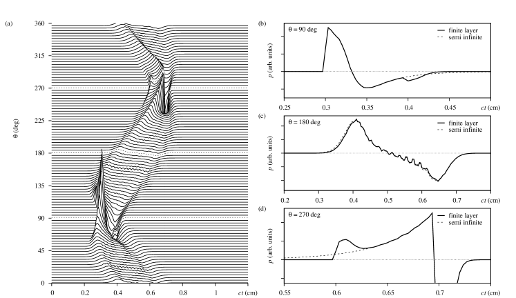
Figure 1: Numerical experiments to model OA signals resulting from the absorption of laser light by a homogeneously absorbing layer. (a) stacked plot of signals resulting from measurements via 100 point detectors arranged as a circular array enclosing the region of interest. The distinguished signals at $\theta=90^{\circ}$, $180^{\circ}$, and $270^{\circ}$ (indicated as dashed lines) are shown in more detail in the subsequent subplots. (b) backward mode signal ($\theta=90^{\circ}$) recorded in the early farfield at $D=1.11$, (c) side-view recorded at $\theta=180^{\circ}$, and, (d) forward mode signal ($\theta=270^{\circ}$) recorded in the farfield at $D=2.22$.

During the course of their propagation, the initial acoustic stress profiles $p_{\rm 0}(\vec{r})$ experience a shape change induced by diffraction, dispersion, acoustic attenuation and nonlinear acoustic effects [3]. In the remainder we restrict our discussion to the shape transformation due to diffraction, which, for the considered laser intensities and material properties is assumed to be dominant. The characteristic features of OA signals are sensitive to the geometric subtleties of the ISP and on the precise detection setup, i.e. the detector-to-sample distance and the geometry and spatial extend of the detection device. In principle one can distinguish two main detection regimes: the acoustic nearfield, wherein an initially plane acoustic wavefront is considered to be of plane wave type, and the acoustic farfield, wherein the wavefront is considered to effectively assume a spherical shape. Both might be distinguished using the dimensionless diffraction parameter

$$D=\frac{|z_{\rm D}|\lambda_{\rm{ac}}}{r_{\rm 0}^{2}},$$ (6)

with detector-to-sample distance $|z_{\rm{D}}|$, beam diameter $r_{0}$ (here interpreted as the $1/e$-intensity threshold of the flat-top ISP in Eq. (3), i.e. subsequently $r_{0}\equiv a_{0}+d_{0}$) and characteristic acoustic wavelength $\lambda_{\rm{ac}}$ [3], which, in stress confinement reads $\lambda_{\rm{ac}}=2\,\mu_{\rm{eff}}^{-1}$. Subsequently, we consider a single absorbing layer in between optically transparent layers, thus we here assume the effective attenuation coefficient $\mu_{\rm{eff}}\equiv\mu_{a}$. Near- and farfield conditions are realized for $D<1$ and $D>1$, respectively.

So as to facilitate intuition regarding the generic features of OA signals, Fig. 1 illustrates a sequence of simulated excess pressure curves. The simulation setup reads as follows: (i) as source volume we consider a $3$D mesh with side lengths $(L_{x},L_{y},L_{z})=(1\,{\rm cm},1\,{\rm cm},1\,{\rm cm})$ and $(N_{x},N_{y},N_{z})=(900,900,300)$ mesh points. Therein, a single absorbing layer (tangent vectors $\vec{e}_{x}$ and $\vec{e}_{y}$) with homogeneous absorption coefficient $\mu_{a}=24\,{\rm cm}^{-1}$ extends from $z=0-0.1\,{\rm cm}$. (ii) as irradiation source we consider a flat-top laser beam as described by Eq. (3) with beam parameters $a_{0}=0.1\,{\rm cm}$ and $d_{0}=a_{0}/2$, i.e. $1/e$-intensity threshold $r_{0}=0.15\,{\rm cm}$. The symmetry axis of the beam is considered to coincide with the $z$-axis, defining a plain normal irradiation scenario. (iii) an array of $100$ point detectors is arranged along a circle with center $(x_{\rm c},y_{\rm c},z_{\rm c})=(L_{x}/2,L_{y}/2,0.2\,{\rm cm})$ and radius $R=0.5\,{\rm cm}$ in the $xz$-plane, surrounding the region of the source volume with nonzero $p_{0}(\vec{r})$. The individual detector positions are generated following $(x_{\rm D},y_{\rm D},z_{\rm D})=(x_{\rm c}+R\cos(\theta),L_{y}/2,z_{\rm c}-R\sin(\theta))$ with $\theta$ in increments of $2\pi/100$. For convenience, since we are only interested in the generic shape of the waveforms as function of $\theta$, we set $c=0.15\,{\rm cm/\mu s}$, $f_{0}=1\,{\rm J/cm^{2}}$ and $\Gamma=1$.

Fig. 1(a) shows a stacked representation of the sequence of measurements recorded using the circularly arranged point detectors. As evident from the figure, both, the signal amplitude and the waveform change as function of $\theta$. The distinct signal shapes can be explained by the relative orientation of the detection point and Beer-Lambert absorption profile within the source volume. The three measurement angles $\theta=90^{\circ}$ (backward mode), $\theta=180^{\circ}$ (side-view), and $\theta=270^{\circ}$ (forward mode), distinguished as dashed lines in the plot, are detailed in Figs. 1(b-d). In backward mode the detection point is located at $D=1.11$, thus observing a borderline farfield signal (solid line). As can be seen from Fig. 1(b) it consists of an initial compression peak, indicating the beginning of the absorbing layer, followed by an extended rarefaction phase and a pronounced rarefaction dip, marking the end of the absorbing layer as evident from a comparison to the simulation result for a semi-infinite layer (indicated by the dashed line in Fig. 1(b)). These are the characteristic features that allow for OA depth profiling in the acoustic far field. Further exemplary backward mode signals in the acoustic near and farfield can be found in numerical experiments $1$ and $2$ detailed in A. In the side-view at $\theta=180^{\circ}$ the numerical procedure yields a quite symmetric bipolar signal, see Fig. 1(c), and in forward mode at $\theta=270^{\circ}$ a sequence of compression peaks terminated by a strong rarefaction phase is visible, see Fig. 1(d). A further exemplary forward mode signal can be found in numerical experiment $3$ in A. Note that in this case, the initial compression peak is due to the finite extend of the absorbing layer and the signal is observed in the farfield at $D=2.22$. Further, note that while the signal features in $\theta=90^{\circ}$ and $270^{\circ}$ reflect the width of the absorbing layer, the side-view at $\theta=180^{\circ}$ relates to the width of the illuminated region.

Subsequently, we report on both, laboratory experiments and numerical simulations that were carried out to better understand the features of OA signals resulting from the absorption of laser energy by melanin enriched elastic solids. Following the formal decomposition of the problem of OA signal generation, the numerical simulation were performed by (i) modelling the optical properties of the computational domain guided by the experimental setup, (ii) considering the absorption of laser light within the source volume, and, (iii) solving the stress wave propagation problem for a medium with homogeneous acoustic properties. In order to benchmark our research code we first replicated several laboratory experiments on liquid dye solution reported in the literature and illustrated in A. Note that while there are further numerical approaches that yield OA signals and their diffraction characteristics in terms of a simplified $1$D approach [24, 25], see B, we prefer the presented voxelized $3$D representation of the source volume since it allows to model custom beam profiles and also more intricate absorbing structures. Further, note that a similar approach for coupling the optical deposition and acoustic propagation problem has been discussed by Ref. [26].

3 OA signals in PVA hydrogel phantoms

As reviewed recently in Ref. [27], ideal phantoms for photoacoustic imaging should meet several criteria in order to ascertain tissue-realistic photoacoustic properties and fabrication reproducibility. Here, in our combined experimental and numerical study we consider polyvinyl alcohol based hydrogel (PVA-H) phantoms [28, 29]. Albeit the preparation procedure of the PVA-H phantoms is rather extensive, as evident from the detailed preparation protocol to yield melanin enriched tissue phantoms summarized in Ref. [11], we appreciate their structural rigidity and tissue-like acoustic properties, rendering them a suitable tool to mimic soft tissue in ultrasound experiments [10] and photoacoustic imaging [9].

In the remainder we complement OA signals measured in PVA-H tissue phantoms consisting of a single, melanin enriched absorbing layer in between optically transparent layers, with numerical calculations resulting from the two-part modelling approach discussed in Section 2. In our experiments, laser pulses were generated using an optical parametric oscillator (NL303G + PG122UV, Ekspla, Lithuania) at a wavelength of $\lambda=532\,{\rm{nm}}$ with pulse duration of approximately $6\,{\rm{ns}}$. After traversing a fiber with $800\,{\rm{\mu m}}$ core diameter (Ceramoptec, Optran WF 800/880N), the beam profile was found to be well described by a flat-top shape, consistent with Eq. (3). For the detection of OA pressure signals, a piezoelectric transducer, consisting of a $9\,{\rm{\mu m}}$ thick piezoelectric polyvinylidenfluorid (PVDF) film with approximately $50\,{\rm{nm}}$ indium tin oxide (ITO) electrodes and an circular active area with radius $r_{\rm D}=0.5\,{\rm{mm}}$, is used [30].

Experiment 1:

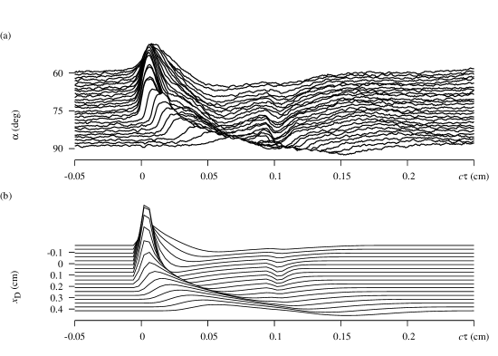
Figure 2: Results of a qualitative study involving laboratory experiments on PVA-H phantoms and custom numerical simulations to predict the expected OA signals. Both figures show normalized OA pressure profiles $p$ (consising of a pronounced compression peak, an extended rarefaction phase and a pronounced rarefaction dip) as function of the retarded signal depth $c\tau$. (a) OA signals measured on a melanin enriched PVA-H phantom with setup paramters reported in the text. Upon decreasing the parameter $\alpha$, the laser spot is shifted across the phantom towards the detector location. (b) OA signals obtained via numerical experiments, modeling the laboratory setup with the parameters reported in the text. Considering plane normal irradiation, $x_{\rm D}$ indicates the deviation of the detector position from the symmetry axis of the beam.

First, we present a qualitative comparative study where we complement measurements, in which a (pulsed) laser beam was scanned across a PVA-H phantom while keeping the detector position fixed, with custom numerical simulations. Albeit the precise implementation of the numerical simulation differs slightly from the laboratory setup, the resulting OA signals can nevertheless be compared on a qualitative basis. To be more precise, in the laboratory setup, the fiber transmitting the laser pulse was hinged above the specimen holder containing the PVA-H phantom. By pivoting the transmitting fiber in an angular range of $\alpha=90$ (plane normal irradiation) through $60$ (inclined irradiation) the illuminated region was shifted across the phantom. In any case, the laserlight entered the phantom close to the detector. To facilitate intuition on the measured OA signals shown in Fig. 2(a), note that the illuminated region approaches the detector as $\alpha$ decreases. During our experiment, the laser spot diameter on the sample surface was approximately $0.3\,{\rm cm}$, defining the lengthscale for the $1/e$-intensity radius for our subsequent numerical simulations. The measurement was performed in backward mode with a distance $z_{\rm D}=1\,{\rm{cm}}$ of the absorbing layer to the detector. The absorbing layer was prepared with thickness $d_{z}=0.1{\rm{cm}}$ and absorption coefficient in the range $\mu_{a}=20-24\,{\rm cm}^{-1}$. I.e. the measurement is performed under farfield conditions at $D=4.4$ (assuming $\mu_{a}=20\,{\rm{cm}}^{-1}$). In Fig. 2(a), the individual signals are shown as function of the time-retarded signal depth $c\tau=ct-z_{\rm D}$ with $c\tau=0$ signifying the start of the absorbing layer. The speed of sound within the PVA-H phantom is assumed to be $c=0.15\,{\rm{cm/\mu s}}$. In the range $\alpha=60\ldots 75$ the initial compression peaks appear at a similar level, indicating the plane part of the acoustic wavefront, resulting from the high-intensity part of the laser spot. In the range $\alpha=75\ldots 90$, a spherical bending of the wavefront due to diffraction can be observed, causing the excess pressure peaks to reach the detector position with some delay, manifested as a peak position at $c\tau>0$. Note that for an extended range of $\alpha$, a pronounced rarefaction dip at $c\tau\approx 0.1\,{\rm{cm}}$ indicates the end of the absorbing layer.

Figure 3: Measurement and numerical simulation of OA signals resulting from the absorption of laser light by a PVA-H phantoms. (a) The main plot shows measured (labeled “M”) and computed (labeled “T”) nearfield signals recorded in backward mode and the inset illustrates a fit using a simple exponential function as discussed in the text, (b) measured and computed farfield signals obtained for a side-view configuration, (c) the main plot shows measured and computed nearfield signals and the inset illustrates a fit using two different exponential fitting functions discussed in the text.

For our custom numerical simulations shown in Fig. 2(b) we consider a pointlike detector (initial numerical experiments suggested that for the given farfield configuration, the spatial extend of the detector can be neglected), a flat-top ISP with beam parameters $a_{0}=0.15\,{\rm{cm}}$ and $a_{0}/d_{0}=2$ and a homogeneous absorption coefficient of $\mu_{a}=20\,{\rm{cm}}^{-1}$ across the $0.1\,{\rm{cm}}$ thick absorbing layer. Further, in contrast to the experimental setup, plain normal laser irradiation was assumed with $x_{\rm D}$ (see Fig. 2(b)) describing the deviation of the detector position from the symmetry axis of the beam. As evident from Fig. 2, the OA signals of the laboratory experiments and numerical simulations agree well on a qualitative basis.

Experiment 2:

In Fig. 3(a) we illustrate a comparison of both, measurement and numerical simulation, for a nearfield signal recorded in backward mode. To summarize the experiment: we considered an absorbing layer of thickness $0.1\,{\rm{cm}}$ and absorption coefficient $\mu_{a}=20-24\,{\rm{cm}}^{-1}$, the diameter of the laser spot was estimated as $0.4\,{\rm{cm}}$ and the detector was positioned at a distance of $0.2\,{\rm cm}$ from the absorbing layer. As can be seen from the figure, the initial compression phase in the signal range $ct=0.2-0.3\,{\rm{cm}}$ follows a Beer-Lambert decay, see Eq. 2, and experiment and simulation agree well. However, note that the geometry of the diffraction induced rarefaction phase is not well represented by the strict flat-top ISP modeled using the parameters $a_{0}=0.21\,{\rm{cm}}$ and $a_{0}/b_{0}=2$. As shown in the inset of Fig. 3(a), anticipating a Beer-Lambert decay and fitting an exponential function $f_{\rm{FIT}}(x)=a\exp[-\mu_{a}^{\prime}c(t-t_{0})]$ to the data in the range $ct\in(0.21,0.28)$, yields the fit parameters $a=O(1)$, $\mu_{a}^{\prime}=22.1(2)\,{\rm{cm}}^{-1}$ and $ct_{0}\approx 0.20$ (the latter reflecting that we here show OA signals where the initial compression peak is normalized to unit height).

Experiment 3:

In Fig. 3(b) we show a custom simulation for an OA signal measured in a side-view configuration (similar to Fig. 1(c)). The measurement was performed at an approximate distance of $1.7\,{\rm{cm}}$ to the narrow laser spot which had a diameter of approximately $0.05\,{\rm{cm}}$. For the numerical experiments we used a flat-top ISP with beam parameters $a_{0}=0.022\,{\rm{cm}}$ and $a_{0}/b_{0}=2$. This measurement was taken out of a sequence of experiments on tissue phantoms with a somewhat lower absorption coefficient of $\mu_{a}\approx 1\,{\rm cm}^{-1}$. Note that while both, the theoretical and experimental signal exhibit a bipolar shape, the latter appers to be more rugged. This effect is most likely due to signal reflections within the PVA-H backing layer used to terminate the PVDF transducer.

Experiment 4:

Finally, in Fig. 3(c) we show an OA signal recorded in forward mode, where the detector is located at a distance of $0.35\,{\rm cm}$ below the beginning of the absorbing layer. The layer itself has a thickness of $0.15\,{\rm{cm}}$, i.e. $z_{D}=0.2\,{\rm{cm}}$, and an absorption coefficient of $\mu_{a}=20-24\,{\rm cm}^{-1}$. During the experiment, the laser spot had a diameter of approximately $0.2\,{\rm cm}$. For the numerical experiments we used the flat-top beam parameters $a_{0}=0.1\,{\rm{cm}}$ and $a_{0}/b_{0}=2$ as well as $\mu_{a}=24\,{\rm{cm}^{-1}}$. I.e., simulations are performed in the acoustic near field at $D=0.74$ The steep increase of the pressure signal in the range $ct\in(0.2\,{\rm cm},0.35\,{\rm cm})$ is in agreement with a Beer-Lambert law as seen from the detector position in forward mode. The finite size of the laser beam is responsible for the strong rarefaction phase in the range $ct\in(0.35\,{\rm cm},0.45\,{\rm cm})$. In principle, experiment and simulation agree quite well. Note that, as in experiment 1 above, it is possible to extract the absorption coefficient from the measured data. Considering a simple exponential increase of the pressure signal in the compression range already yields $\mu_{a}^{\prime}=21.0(1)\,{\rm cm}^{-1}$. An effective fitting function of the form $g_{\rm{FIT}}=a_{0}+a_{1}\exp[\mu_{a}^{\prime}c(t-t0)]$, allowing to also account for an initial “flat” part of the compression phase yields the fit parameter $a_{0}=O(10^{-1})$, $a_{1}=O(1)$, $ct_{0}\approx 0.36$, and $\mu_{a}^{\prime}=23.7(2)\,{\rm cm}^{-1}$, in reasonable agreement with the expected range of $\mu_{a}$.

4 Summary and Conclusions

We presented a combined study, complementing measured OA signals with custom numerical simulations. The laboratory experiments where performed on melanin enriched PVA-H phantoms, i.e. elastic solids that possess tissue-like acoustic properties and are used to mimic soft tissue in ultrasound experiments and photoacoustic imaging [10, 9]. Since the experimental conditions satisfy the limits of stress confinement, the problem of OA signal generation decouples into the processes of laser absorption and stress wave propagation that can be approached separately. Consequently, numerical simulations were performed by: (i) modelling the optical properties of the computational domain, (ii) considering the absorption of laser light within the source volume, and, (iii) solving the stress wave propagation problem for a medium with homogeneous acoustic properties using the optoacoustic Poisson integral. So as to benchmark our research code we first replicated several laboratory experiments on liquid dye solution reported in the literature, see A. Complementing a recent study wherein we elaborated on the detection, numerical simulation and approximate inversion of OA signals [11], we here apply the procedure to model OA near- and farfield signals observed in experiments on PVA-H phantoms. Overall we found a good qualitative agreement between both. In the acoustic nearfield we found that the initial excess pressure profile could be modeled well using the parameters of the respective experiments, however, the precise shape of the subsequent rarefaction phase differed from that recorded in the experiment, see Figs. 3(a,c). In this regard, note that here the focus is on modelling the principal shape of the OA signal. We did, however, make no attempt at modelling the behavior of the PVDF-based transducer used in the laboratory setup (as previousely done for a similar detection device, see Ref. [12]). Further, note that a fit of simple model functions to the compression phases in experiments 2 and 4, see Figs. 3(a,c), allowed to obtain estimates of the absorption coefficients for the absorbing layers from the measurement. The resulting estimates are in good agreement with the values expected on basis of the phantom preparation procedure.

Appendix A Numerical simulation of OA signals measured on dye solution

Subsequently we illustrate the numerical calculation of OA signals that result from the absorption of laser light in liquid samples, consisting of a layer of light absorbing dye solution in between layers of optically transparent liquid, for three different experimental setups reported in the literature. We replicated these studies by numerical means for benchmarking our research code.

Numerical experiment 1:

In Ref. [32], the authors report on an experimental study, where they observed near and far field signals using an optical detector for the measurement of acoustic stress waves. The detector was operated in reflection mode, similar to the backward mode used in our study. Keeping the sample to detector distance constant and tuning the width of the flat-top profile of the HeNe laser used in their setup, they were able to record OA signals in both measurement regimes. In Figs. 4(a,b) we illustrate numerical simulations geared towards the laboratory experiments reported in Ref. [32]. Therefore, we considered a computational domain modeling an absorbing layer of width $w=300\,\mu{\rm m}$ and absorption coefficient $\mu_{a}=13\,\rm{cm}^{-1}$ (i.e. weakly absorbing scenario at $\lambda=550\,{\rm nm}$; see Fig. 4(a)) and $\mu_{a}=80\,\rm{cm}^{-1}$ (i.e. strongly absorbing scenario at $\lambda=532\,{\rm nm}$; see Fig. 4(b)) for diffraction parameters $D=0.16$ and $D=4$ at a sample to detector distance of $|z_{\rm D}|=1.2\,{\rm mm}$, referring to the acoustic near field and far field of the measurement setup, respectively. Note that the small peak at the signal depth $\approx 600\,{\rm\mu m}$ in Fig. 8b of Ref. [32], resulting from acoustic reflection at the plastic container walls that separate the distinct liquid layeres, is not modeled by our approach. Further, note that the above laboratory experiments where reported using normalized optoacoustic signals wherein the initial excess pressure peak has unit height. Hence, the numerical simulations tailored towards those experiments are normalized in the same manner to facilitate a compoarison of both.

Figure 4: Numerical experiments to model OA signals resulting from the absorption of laser light in liquid samples, consisting of a layer of dye solution in between layers of optically transparent liquid. The subfigures refer to the laboratory experiments reported in (a) Fig. 8(a) of ref. [32], (b) Fig. 8(b) of ref. [32], (c) Fig. 3(a) of ref. [33] and Figs. 5 and 6 of ref. [13], (d) Fig. 2(b) of ref. [23]. Details on the setup of the simulation domain can be found in A.

Numerical experiment 2:

In contrast to the previous numerical experiment, where the reference curves consist of normalized excess pressure signals, a further study reported in Refs. [33, 13] allows to compare a custom numerical simulation to an actual pressure signal recorded in the acoustic near field in reflection mode. The corresponding measurement setup reported in the above references consists of an (calibrated) optical stress detector and a Nd:YAG laser at wavelength $\lambda=532\rm{nm}$ with $H_{0}=0.18\,{\rm J/m}$ and flat-top ISP parameters $a_{0}=1.94\,{\rm mm}$ and $d_{0}=0.43\,{\rm mm}$, incident onto a layer of dye solution characterized by a Grüneisen paremeter $\Gamma=0.11$ and absorption coefficient $\mu_{a}=24\,{\rm cm}^{-1}$ at a sample to detector distance of $|z_{\rm D}|=1\,{\rm mm}$ (see Fig. 5 of Ref. [33]). Further, Ref. [33] reports several normalized OA signals resulting from different values for the diameter of the flat-top laser profile to illustrate the change in signal shape during the transition from the acoustic near field to the far field (see Fig. 6 of Ref. [33]). Our numerical simulations geared towards those experimets are shown in Fig. 4(c).

Numerical experiment 3:

As a further challenge we considered the laboratory experiments reported in Ref. [23]. Therein, two sets of experiments with varying detector and beam-width combinations where reported. Among those, a piezoelectronic ITO transducer (similar to the one used in our experimental setup) was used to record OA signals in forward mode. In detail, our numerical simulations consider a circular ITO detector with diameter of $r_{\rm D}=3\,{\rm mm}$ placed at a distance of $z_{\rm D}=2.25\,{\rm mm}$ of a dye layer with width $w=0.9\,{\rm mm}$ and absorption coefficient $\mu_{a}=1.65\,{\rm mm}^{-1}$. As irradiation source, the laboratory setup in Ref. [23] used a Nd:YAG laser (operating at $\lambda=577\,{\rm nm}$) to obtain a homogeneous circular ISP with a radius of $r_{0}=3\,{\rm mm}$. For this particular setup, the resulting OA signal is strongly distorted by diffraction, causing an extended rarefaction phase subsequent to the initial raise of the excess pressure profile expected by Beers law (see Fig. 2 of Ref. [23]). In order to model these signal features properly, the spatial extend of the detector has to be taken into account via integrating the excess pressure signal numerically over an appropriate circular area. A sequence of numerical simulations that illustrate the corresponding OA signal for different detector radii is illustrated in Fig. 4(d). Note that, while Ref. [23] quotes a homogeneous circular beam profile with $r_{0}=3\,{\rm mm}$, corresponding to a sharp flat-top ISP, we observed that a more realistic and smooth flat-top ISP with $1/e$-intensity radius $r_{0}$ and beam profile parameters $r_{0}=a_{0}+d_{0}$, where $a_{0}/d_{0}=4$, reproduces the curves observed by Jaeger et al. best. Further, note that while the results reported by Jaeger et al. refer to the transducer response measured in ${\rm mV}$, our simulation results are normalized to a peak pressure height of unity.

Appendix B Comparison of $3$D simulations to effectively $1$D approaches

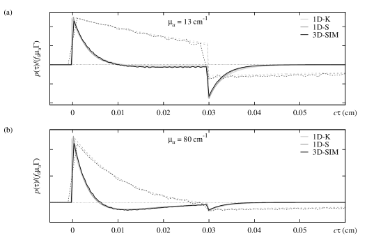
Figure 5: Comparison of fully voxelized $3$D simulations using a Gaussian beam profile (labeled “$3$D-SIM”), following the simulation protocol discussed in sec. 2, to $1$D approaches that model the effect of acoustic diffraction under the assumption of plane acoustic waves and a Gaussian beam profile, see discussion in B. The curves labeled “$1$D-K” and “$1$D-S” result from numerical simulations using the theoretical frameworks discussed by Ref. [25] and Refs. [24, 3], respectively. The source volume configuration is similar to the one discussed in terms of numerical experiment $1$ in A, i.e. (a) $\mu_{a}=13\,{\rm cm}^{-1}$, and (b) $\mu_{a}=80\,{\rm cm}^{-1}$. In both subfigures solid (dashed) lines refer to the farfield (nearfield) scenario considering a Gaussian ISP with $1/e$-intensity threshold of $a_{0}=1.5\,{\rm mm}$ ($a_{0}=0.3\,{\rm mm}$).

As pointed out in sec. 2, we follow a numerical approach that might be summarized as a three-step procedure: (i) modelling the optical properties of a $3$D computational domain, (ii) considering the absorption and scattering of laser light within the source volume, and, (iii) solving the stress wave propagation problem for a medium with homogeneous acoustic properties via the OA Poisson integral Eq. (5). While this is a quite versatile $3$D approach that allows to model custom beam profiles and intricate absorbing structures, note that there exist also effectively $1$D approaches that yield OA waveforms under certain simplifying assumptions. Here we consider two $1$D theoretical approaches, both based on the solution of convolution integrals and valid under the assumption of plane acoustic waves and Gaussian beam profiles. Albeit these simplified approaches allow to obtain closed form analytic OA signals, we here solve the respective equations numerically for the source volume configuration discussed in terms of numerical experiment $1$ in A. These simplified calculations serve as limiting cases to which we compare our fully $3$D simulations, again allowing for benchmarking our research code. Below, both one-dimensional approaches are briefly discussed.

$1{\rm{D}}$ approach due to Karabutov et al.:

Considering the paraxial approximation of the $3$D acoustic wave equation and assuming a transverse Gaussian ISP $f(\vec{r}_{\perp})=\exp(-|\vec{r}_{\perp}|^{2}/a_{0}^{2})$, the diffraction transformation of OA signals at the detection point $z$ along the beam axis (i.e. $\vec{r}_{\perp}=0$) can be can be related to the unperturbed on-axis pressure profile $p_{\rm 0}(\tau)$ (wherein $\tau=t-z/c$) via a linear convolution integral, reading [25]

$$p(\tau)=p_{\rm 0}(\tau)-\omega_{\rm D}\int_{-\infty}^{\tau}\!\mathsf{K}(\tau-\tau^{\prime})\,p_{\rm 0}(\tau^{\prime})\,\mathrm{d}\tau^{\prime}.$$ (7)

Therein the convolution kernel $\mathsf{K}(\tau-\tau^{\prime})=\exp\{-\omega_{a}zL_{\rm D}^{-1}(\tau-\tau^{\prime})\}$ governs the diffraction transformation of the propagating acoustic stress waves, depending on the characteristic frequency $\omega_{a}=c\mu_{a}$ of the OA signal spectrum and the diffraction length $L_{\rm D}=\pi a_{0}^{2}/\lambda$, defined by the acoustic wavelength $\lambda=2\pi/\mu_{a}$. Using the normalized initial stress profile $p_{\rm 0}(\tau)=\exp\{-\mu_{a}c\tau\}$, nonzero in the range $c\tau\in[0\,{\rm mm},0.3\,{\rm mm}]$, and the parameters $c=1.5\,{\rm mm/\mu s}$ as well as $\mu_{a}$ and $a_{0}$ as reported by Ref. [32], cf. numerical experiment $1$ in A, we yield the curves labeled by “$1$D-K” in Fig. 5.

$1{\rm{D}}$ approach due to Sigrist et al.:

A quite similar one-dimensional theoretical approach, build upon the assumption of plane acoustic wave propagation, yields the convolution integral [3, 24]

$$p_{r}(\tau)=\omega_{a}\int_{-\infty}^{\infty}\!\mathsf{K}(\tau-\tau^{\prime})\,p_{\rm 0}(\tau^{\prime})\,\mathrm{d}\tau^{\prime},$$ (8)

by means of which the diffraction altered excess pressure profile $p_{r}(\tau)$ for a rigid (i.e. motionless) boundary can be related to the unperturbed stress profile $p_{\rm 0}(\tau)$. In our case, the more interesting excess pressure profile $p(\tau)$ for a free (i.e. pressure-release) boundary is related to $p_{r}(\tau)$ simply via $p(\tau)=\omega_{a}^{-1}\frac{d}{d\tau}p_{r}(\tau)$. While the convolution kernel ${\mathsf{K}}$ is formally similar to the one introduced previously, the definition of the diffraction length is slightly different, i.e. $L_{\rm D}=2\pi d^{2}/\lambda^{\prime}$. Now, so as to treat both one-dimensional frameworks under similar conditions, we effectively match parameters by considering the acoustic wavelength used in Ref. [25], i.e. $\lambda^{\prime}\equiv 2\pi/\mu_{a}$, and setting the beam parameter $d\equiv a_{0}/\sqrt{2}$. The latter is in agreement with the definition of $d$ as the diameter of the (Gaussian) beam spot with radial profile $f^{\prime}(\vec{r}_{\perp})=\exp(-2|\vec{r}_{\perp}|^{2}/d^{2})$, see [3]. Using the initial stress profile $p_{\rm 0}(\tau)$ and simulation parameters $c$, $\mu_{a}$ and $a_{0}$ as above, we yield the curves labeled by “$1$D-S” in Fig. 5.

First, note that the numerical results of the fully $3$D simulations via a Gaussian beam profile agree very well with the effectively $1$D approaches based on the additional assumption of plane acoustic wave propagation. The latter assumption in principle requires a setup in which $\mu_{a}a_{0}\gg 1$, a condition best satisfied for Fig. 5(b). The deviation of the data curves close to the steep increase and decrease of the pressure profile are solely due to the coarse mesh structure used in the $3$D approach. Further, note that the simplified calculations in terms of purely Gaussian beam profiles reproduce the compression and rarefaction characteristics of the farfield signals seen in Figs. 8(a,b) of Ref. [32] quite well, see the solid lines in Figs. 5(a,b). However, they cannot account for the characteristic shape of the extended rarefaction phase caused by the lateral limits of the beam profile observed for the nearfield signals in Ref. [32], see the dashed lines in Figs. 5(a,b). In contrast, note that the fully $3$D simulations using a custom flat-top beam profile reported in A reproduce the experiments of Ref. [32] satisfactorily.

References

References

- [1] R. A. Kruger, P. Liu, Y. Fang, and C. R. Appledorn. Photoacoustic ultrasound (paus) - reconstruction tomography. Med. Phys., 22:1605–1609, 1995.
- [2] M. W. Sigrist and F. K. Kneubühl. Laser-generated stress waves in liquids. J. Acoust. Soc. Am., 64(6):1652–1663, 1978.
- [3] M. W. Sigrist. Laser generation of acoustic waves in liquids and gases. J. Appl. Phys., 60:R83–R122, 1986.
- [4] D. A. Hutchins. Mechanisms of pulsed photoacoustic generation. Can. J. Phys., 64(9):1247–1264, 1986.
- [5] A. C. Tam. Applications of photoacoustic sensing techniques. Rev. Mod. Phys., 58:381–431, 1986.
- [6] G. J. Diebold, M. I. Khan, and S. M. Park. Photoacoustic signatures of particulate matter: optical production of acoustic monopole radiation. Science, 250(4977):101–104, 1990.
- [7] G. J. Diebold, T. Sun, and M. I. Khan. Photoacoustic monopole radiation in one, two, and three dimensions. Phys. Rev. Lett., 67:3384–3387, 1991.
- [8] L.V. Wang. Photoacoustic Imaging and Spectroscopy. Optical Science and Engineering. CRC Press, 2009.
- [9] W. Xia, D. Piras, M. Heijblom, W. Steenbergen, T. G. Van Leeuwen, and S. Manohar. Poly(vinyl alcohol) gels as photoacoustic breast phantoms revisited. J. Biomed. Opt., 16(7):075002–075002, 2011.
- [10] K. Zell, J. I. Sperl, M. W. Vogel, R. Niessner, and C. Haisch. Acoustical properties of selected tissue phantom materials for ultrasound imaging. Phys. Med. Biol., 52(20):N475, 2007.
- [11] E. Blumenröther, O. Melchert, M. Wollweber, and B. Roth. Detection, numerical simulation and approximate inversion of optoacoustic signals generated in multi-layered PVA hydrogel based tissue phantoms. Photoacoustics, 4:125–132, 2016.
- [12] M. G. González, P. A. Sorichetti, and G. D. Santiago. Modeling thin-film piezoelectric polymer ultrasonic sensors. Rev. Sci. Instrum., 85(11):115005, 2014.
- [13] G. Paltauf and H. Schmidt-Kloiber. Measurement of laser-induced acoustic waves with a calibrated optical transducer. J. Appl. Phys., 82:1525, 1997.
- [14] S. L. Jacques. Optical properties of biological tissue: a review. Phys. Med. Biol., 58:R37–R61, 2013.
- [15] L. Wang, S. L. Jacques, and L. Q. Zheng. MCML - Monte Carlo modeling of photon transport in multi-layered tissues. Comput. Methods Progr. Biomed., 47:131, 1995.
- [16] E. Alerstam, W. C. Y. Lo, T. D. Han, J. Rose, S. Andersson-Engels, and L. Lilge. Next-generation acceleration and code optimization for light transport in turbid media using gpus. Biomed. Opt. Express, 1:658–675, 2010.
- [17] L. Wang, S. L. Jacques, and L. Q. Zheng. CONV - convolution for responses to a finite diameter photon beam incident on multi-layered tissues. Comput. Methods Progr. Biomed., 54:141, 1997. For source code, see: http://omlc.org/software/mc/.
- [18] O. Melchert, M. Wollweber, and B. Roth. Efficient polar convolution based on the discrete Fourier-Bessel transform for application in computational biophotonics. (unpublished), 2016.
- [19] S. L. Jacques and T. Li. Monte Carlo simulations of light transport in 3D heterogeneous tissues (mcxyz.c). See http://omlc.org/software/mc/mcxyz/index.html [accessed 30.01.2017], 2013.
- [20] V. E. Gusev and A. A. Karabutov. Laser Optoacoustics. American Institute of Physics, 1993.
- [21] D.-K. Yao, C. Zhang, K. Maslov, and L. V. Wang. Photoacoustic measurement of the Grüneisen parameter of tissue. J. Biomed. Opt., 19(1):017007–017007, 2014.
- [22] H. Schoeffmann, H. Schmidt-Kloiber, and E. Reichel. Time-resolved investigations of laser-induced shock waves in water by use of polyvinylidenefluoride hydrophones. J. Appl. Phys., 63:46–51, 1988.
- [23] M. Jaeger, J. J. Niederhauser, M. Hejazi, and M. Frenz. Diffraction-free acoustic detection for optoacoustic depth profiling of tissue using an optically transparent polyvinylidene fluoride pressure transducer operated in backward and forward mode. J. Biomed. Opt., 10(2):024035, 2005.
- [24] M. Terzić and M. W. Sigrist. Diffraction characteristics of laser-induced acoustic waves in liquids. J. Appl. Phys., 56(1):93–95, 1984.
- [25] A. Karabutov, N. B. Podymova, and V. S. Letokhov. Time-resolved laser optoacoustic tomography of inhomogeneous media. Appl. Phys. B, 63:545–563, 1996.
- [26] S. L. Jacques. Coupling 3d monte carlo light transport in optically heterogeneous tissues to photoacoustic signal generation. Photoacoustics, 2:137–142, 2014.
- [27] M. Fonseca, B. Zeqiri, P. C. Beard, and B. T. Cox. Characterisation of a phantom for multiwavelength quantitative photoacoustic imaging. Phys. Med. Biol., 61(13):4950, 2016.
- [28] A. Kharine, S. Manohar, R. Seeton, R. G. M. Kolkman, R. A. Bolt, W. Steenbergen, and F. F. M. deMul. Poly(vinyl alcohol) gels for use as tissue phantoms in photoacoustic mammography. Phys. Med. Biol., 48(3):357–370, 2003.
- [29] M. Meinhardt-Wollweber, C. Suhr, A.-K. Kniggendorf, and B. Roth. Tissue phantoms for multimodal approaches: Raman spectroscopy and optoacoustics. In SPIE BiOS, SPIE Proceedings, page 89450B. SPIE, 2014.
- [30] J. J. Niederhauser, M. Jaeger, M. Hejazi, H. Keppner, and M. Frenz. Transparent ito coated pvdf transducer for optoacoustic depth profiling. Optics Communications, 253(4-6):401–406, 2005.
- [31] O. Melchert. PyPCPI - A python module for optoacoustic signal generation via polar convolution and Poisson integral evaluation. See https://github.com/omelchert/PCPI.git [accessed 15.02.2017], 2016.
- [32] G. Paltauf and H. Schmidt-Kloiber. Pulsed optoacoustic characterization of layered media. J. Appl. Phys., 88:1624–1631, 2000.
- [33] G. Paltauf, H. Schmidt-Kloiber, and H. Guss. Light distribution measurements in absorbing materials by optical detection of laser-induced stress waves. Appl. Phys. Lett., 69(11):1526–1528, 1996.