Fully packed loop configurations: polynomiality and nested arches

Abstract.

This article proves a conjecture by Zuber about the enumeration of fully packed loops (FPLs). The conjecture states that the number of FPLs whose link pattern consists of two noncrossing matchings which are separated by $m$ nested arches is a polynomial function in $m$ of certain degree and with certain leading coefficient. Contrary to the approach of Caselli, Krattenthaler, Lass and Nadeau (who proved a partial result) we make use of the theory of wheel polynomials developed by Di Francesco, Fonseca and Zinn-Justin. We present a new basis for the vector space of wheel polynomials and a polynomiality theorem in a more general setting. This allows us to finish the proof of Zubers conjecture.

1. Introduction

Alternating sign matrices (ASMs) are combinatorial objects with many different faces. They were introduced by Robbins and Rumsey in the 1980s and arose from generalizing the determinant. Together with Mills, they [9] conjectured a closed formula for the enumeration of ASMs of given size, first proven by Zeilberger [12]. Using a second guise of ASMs, the six vertex model, Kuperberg [8] could find a different proof for their enumeration. A more detailed account on the history of the ASM Theorem can be found in [2].

A third way of looking at ASMs are fully packed loops (FPLs). We obtain by using the FPL description a natural refined counting $A_{\pi}$ of ASMs by means of noncrossing matchings. Razumov and Stroganov [10] conjecturally connected FPLs to the $O(1)$ loop model, a model in statistical physics. Proven by Cantini and Sportiello [3], this connection allows a description of $(A_{\pi})_{\pi\in\textnormal{NC}_{n}}$ as an eigenvector of the Hamiltonian of the $O(1)$ loop model, where $\textnormal{NC}_{n}$ is the set of noncrossing matchings of size $n$. Assuming the (at that point unproven) Razumov-Stroganov conjecture to be true, Zuber [15] formulated nine conjectures about the numbers $A_{\pi}$. In this paper we finish the proof of the following conjecture.

Theorem 1 ([15, Conjecture $7$]).

For noncrossing matchings $\pi_{1}\in\textnormal{NC}_{n_{1}},$ $\pi_{2}\in\textnormal{NC}_{n_{2}}$ and an integer $m$, the number of FPLs with link pattern $(\pi_{1})_{m}\pi_{2}$ is a polynomial in $m$ of degree $|\lambda(\pi_{1})|+|\lambda(\pi_{2})|$ with leading coefficient $\frac{f_{\lambda(\pi_{1})}f_{\lambda(\pi_{2})}}{|\lambda(\pi_{1})|!|\lambda(\pi_{2})|!}$, where $f_{\lambda}$ denotes the number of standard Young tableaux of shape $\lambda$.

Caselli, Krattenthaler, Lass and Nadeau [4] proved this for empty $\pi_{2}$ and showed that $A_{(\pi_{1})_{m}\pi_{2}}$ is a polynomial for large values of $m$ with correct degree and leading coefficient. In this paper we prove that the number $A_{(\pi_{1})_{m}\pi_{2}}$ is a polynomial function in $m$, which is achieved without relying on the work of [4], and hence finish together with the results of [4] the proof of Theorem 1.

We conclude the introduction by sketching the theory on which the proof of Theorem 1 relies and giving an overview of this paper. In the next section we introduce the combinatorial objects and their notions.

As mentioned before the Razumov-Stroganov-Cantini-Sportiello Theorem 5 states that $(A_{\pi})_{\pi\in\textnormal{NC}_{n}}$ is up to multiplication by a constant the unique eigenvector to the eigenvalue $1$ of the Hamiltonian of the homogeneous $O(1)$ loop model. In Section 3 we present that in a special case solutions of the quantum Knizhnik-Zamolodchikov (qKZ) equations lie in the eigenspace to the eigenvalue $1$ of the Hamiltonian of the inhomogeneous $O(1)$ loop model. Di Francesco and Zinn-Justin [5] could characterise the components of these solutions in a different way, namely as wheel polynomials. The specialisation of the inhomogeneous to the homogeneous $O(1)$ loop model means for wheel polynomials performing the evaluation $z_{1}=\ldots=z_{2n}=1$. Summarising, for every $\pi\in\textnormal{NC}_{n}$ there exists an element $\Psi_{\pi}$ of the vector space $W_{n}[z]$ of wheel polynomials such that $A_{\pi}=\Psi_{\pi}(1,\ldots,1)$.

$$\textnormal{FPLs}\mathrel{\mathop{\longleftrightarrow}^{\textnormal{RSCS -- Thm}}}\textnormal{hom }O(1) \mathrel{\mathop{\longleftarrow}^{\textnormal{specialisation}}} \textnormal{inhom }O(1)\mathrel{\mathop{\longleftrightarrow}^{\textnormal{Di F. -- Z.\,J.\,}}} W_{n}[z]$$

$$A_{\pi}=\Psi_{\pi}(1,\ldots,1) \mathrel{\mathop{\longleftarrow}^{\textnormal{evaluation}}} \Psi_{\pi}$$

We introduce a new family of wheel polynomials $D_{\pi_{1},\pi_{2}}$ such that every $\Psi_{\rho^{n_{2}}(\pi_{1}\pi_{2})}$ is a linear combination of $D_{\sigma_{1},\sigma_{2}}$ where $\rho$ is the rotation acting on noncrossing matchings and for $i=1,2$ the Young diagram $\lambda(\sigma_{i})$ is included in the Young diagram $\lambda(\pi_{i})$.

The advantage of the wheel polynomials $D_{\pi_{1},\pi_{2}}$ over $\Psi_{\pi_{1}\pi_{2}}$ becomes clear in Section 4. We prove in Lemma 19 in a more general setting that $D_{\pi_{1},\pi_{2}}(1,\ldots,1)$ is a polynomial function with degree at most $|\lambda(\pi_{1})|+|\lambda(\pi_{2})|$. This lemma applied in our situation and using the rotational invariance $A_{\pi}=A_{\rho(\pi)}$ imply the polynomiality in Theorem 1.

An extended abstract of this work was published in the Proceedings of FPSAC 2016 [1].

2. Definitions

This section should be understood as a handbook of the combinatorial objects involved in this paper.

2.1. Noncrossing matchings and Young diagrams

A noncrossing matching of size $n$ consists of $2n$ points on a line labelled from left to right with the numbers $1,\ldots,2n$ together with $n$ pairwise noncrossing arches above the line such that every point is endpoint of exactly one arch. An example can be found in Figure 1. Denote for two noncrossing matchings $\sigma,\pi$ by $\sigma\pi$ their concatenation. For an integer $n$ we define $(\pi)_{n}$ as the noncrossing matching $\pi$ surrounded by $n$ nested arches, see Figure 2. Define $\textnormal{NC}_{n}$ as the set of noncrossing matchings of size $2n$. It is easy to see that $|\textnormal{NC}_{n}|=C_{n}=\frac{1}{n+1}\binom{2n}{n}$, where $C_{n}$ is the $n$-th Catalan number.

Figure 1. A noncrossing matching $\pi$ of size $3$ and its corresponding Young diagram $\lambda(\pi)$.

Figure 2. The noncrossing matchings $(\pi)$ and $\pi()$ where $\pi$ is the noncrossing matching of Figure 1.

A Young diagram is a finite collection of boxes, arranged in left-justified rows and weakly decreasing row-length from top to bottom. We can think of a Young diagram $\lambda$ as a partition $\lambda=(\lambda_{1},\ldots,\lambda_{l})$, where $\lambda_{i}$ is the number of boxes in the $i$-th row from top. Noncrossing matchings of size $n$ are in bijection to Young diagrams for which the $i$-th row from top has at most $n-i$ boxes for $1\leq i\leq n$. For a noncrossing matching $\pi$ its corresponding Young diagram $\lambda(\pi)$ is given by the area enclosed between two paths with same start- and endpoint. The first path consists of $n$ consecutive north-steps followed by $n$ consecutive east-steps. We construct the second path by reading the numbers from left to right and drawing a north-step if the number labels a left-endpoint of an arch and an east-step otherwise. An example of a noncrossing matching and its corresponding Young diagram is given in Figure 1. For a given noncrossing matching $\pi$ and a positive integer $k$ the Young diagrams $\lambda(\pi)$ and $\lambda((\pi)_{k})$ are the same. To be able to distinguish between them we will always draw the first path of the above algorithm in the pictures of $\lambda(\pi)$.

We define a partial order on the set $\textnormal{NC}_{n}$ of noncrossing matchings via $\sigma<\pi$ iff the Young diagram $\lambda(\sigma)$ is contained in the Young diagram $\lambda(\pi)$. For $2\leq j\leq 2n-2$ we write $\sigma\nearrow_{j}\pi$ if $\lambda(\pi)$ is obtained by adding a box to $\lambda(\sigma)$ on the $j$-th diagonal, where the diagonals are labelled as in Figure 3. This labelling of the diagonals is the second reason for drawing the consecutive north and east steps in the pictures of the Young diagrams.

Figure 3. The matchings $\sigma,\pi$ satisfy $\sigma\nearrow_{2}\pi$.

2.2. The Temperley-Lieb Operators

We define first the rotation $\rho:\textnormal{NC}_{n}\rightarrow\textnormal{NC}_{n}$. Two numbers $i$ and $j$ are connected in $\rho(\pi)$ for $\pi\in\textnormal{NC}_{n}$ iff $i-1$ and $j-1$ are connected in $\pi$, where we identify $2n+1$ with $1$. The Temperley-Lieb operator $e_{j}$ for $1\leq j\leq 2n$ is a map from noncrossing matchings of size $n$ to themselves. For a given $\pi\in\textnormal{NC}_{n}$ the noncrossing matching $e_{j}(\pi)$ is obtained by deleting the arches which are incident to the points $j,j+1$ and adding an arch between $j,j+1$ and an arch between the points former connected to $j$ and $j+1$. Thereby we identify $2n+1$ with $1$. There exists also a graphical representation of the Temperley-Lieb operators. Applying $e_{j}$ on a noncrossing matching $\pi$ is done by attaching the diagram of $e_{j}$, depicted in Figure 4, at the bottom of the diagram of $\pi$ and simplifying the paths to arches. An example for this is given in Figure 5.

Figure 4. The graphical representation of $e_{j}$

Figure 5. Calculating $e_{j}(\pi)$ graphically with $\pi$ from the previous example.

Since noncrossing matchings of size $n$ are in bijection with Young diagrams whose $i$-th row from the top has at most $n-i$ boxes, we can define $e_{j}$ also for such Young diagrams via $e_{j}(\lambda(\pi)):=\lambda(e_{j}(\pi))$. For $1\leq j\leq 2n-1$ the action of $e_{j}$ on Young diagrams is depicted in Figure 6. The operator $e_{2n}$ maps a Young diagram to itself iff the $i$-th row has less than $n-i$ boxes for all $1\leq i\leq n-1$. Otherwise the Young diagram corresponds to a noncrossing matching of the form $(\alpha)\beta(\gamma)$, where $\alpha,\beta,\gamma$ are noncrossing matchings of smaller size. In this case $e_{2n}$ maps this Young diagram to the one corresponding to the noncrossing matching $(\alpha(\beta)\gamma)$, as depicted in Figure 7. The next lemma is an easy consequence of the above observations.

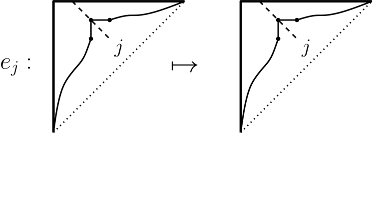
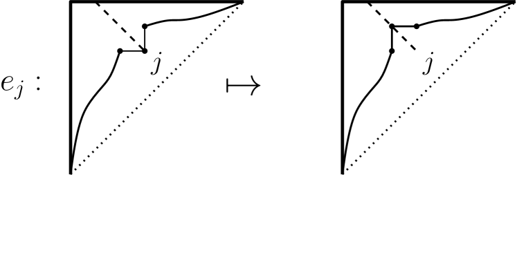
Figure 6. The action of $e_{j}$ for $1\leq j\leq 2n-1$ on Young diagrams corresponding to noncrossing matchings of size $n$.

Figure 7. The action of $e_{2n}$ on Young diagrams corresponding to noncrossing matchings of size $n$ of the form $(\alpha)\beta(\gamma)$, where $\alpha,\beta,\gamma$ are noncrossing matchings.

Lemma 2.

1. For a noncrossing matching $\pi$ of size $n$ and $2\leq j\leq 2n-2$, the preimage $e_{j}^{-1}(\pi)$ is a subset of $\{\sigma|\pi\nearrow_{j}\sigma\}\cup\{\sigma|\sigma\leq\pi\}$.

2. Let $\alpha\in\textnormal{NC}_{n}$, $\beta,\gamma\in\textnormal{NC}_{n^{\prime}}$ be noncrossing matchings such that there exists $2\leq i\leq 2n^{\prime}-2$ with $\beta\nearrow_{i}\gamma$. Then the preimage $e_{2n+i}^{-1}(\alpha\beta)$ is given by

   $$e_{2n+i}^{-1}(\alpha\beta)=\{\alpha\sigma|\sigma\in e_{i}^{-1}(\beta)\}.$$

Proof.

1. If $\pi$ has no arch between $j$ and $j+1$, then $e_{j}^{-1}(\pi)=\emptyset$. Figure 7 displays the action of $e_{j}$ on Young diagrams and implies the statement if $\pi$ has an arch between $j$ and $j+1$.

2. Let $\sigma\in e_{2n+i}^{-1}(\alpha\beta)$ and denote by $x,y$ the labels which are connected in $\sigma$ to $2n+i$ or $2n+i+1$ respectively. By definition of $e_{2n+i}$ the noncrossing matchings $\alpha\beta$ and $\sigma$ differ only in the arches between $2n+i,2n+i+1,x,y$. The existence of an $\gamma$ with $\beta\nearrow_{i}\gamma$ means there exists an arch in $\beta$ with left-endpoint before $i$ and right-endpoint after $i$, hence surrounding $2n+i$ and $2n+i+1$. Therefore $x$ and $y$ must be surrounded by this arch or they are the labels of the points connected by this arch. In both cases $x,y\geq 2n$ which implies $\sigma$ can be written as $\alpha\sigma^{\prime}$ with $e_{i}(\sigma^{\prime})=\beta$. ∎

The Temperley-Lieb algebra with parameter $\tau=-(q+q^{-1})$ of size $2n$ is generated by the Temperley-Lieb operators $e_{i}$ with $1\leq i\leq 2n$ over $\mathbb{C}$. The elements $e_{i},e_{j}$ satisfy for all $1\leq i,j\leq 2n$ the following relations

$$e_{i}^{2} =\tau e_{i},$$

$$e_{i}e_{j} =e_{j}e_{i}\qquad\textit{if }2\leq|(i-j)|\leq 2n-2,$$

$$e_{i}e_{i\pm 1}e_{i} =e_{i}.$$

Throughout this paper we interpret $e_{i}v$ for some vector $v\in\{f|f:\textnormal{NC}_{n}\rightarrow V\}$ and a vector space $V$ always as the action of an element of the Temperley-Lieb algebra on the vector $v$, where the Temperley-Lieb operators act as permutations, i. e., $e_{i}((v_{\pi})_{\pi\in\textnormal{NC}_{n}})=(v_{e_{i}(\pi)})_{\pi\in\textnormal{NC}_{n}}$.

2.3. Fully packed loop configurations

A fully packed loop configuration (or short FPL) $F$ of size $n$ is a subgraph of the $n\times n$ grid with $n$ external edges on every side with the following two properties.

1. All vertices of the $n\times n$ grid have degree $2$ in $F$.

2. $F$ contains every other external edge, beginning with the topmost at the left side.

An FPL consists of pairwise disjoint paths and loops. Every path connects two external edges. We number the external edges in an FPL counter-clockwise with $1$ up to $2n$, see Figure 8. This allows us to assign to every FPL $F$ a noncrossing matching $\pi(F)$, where $i$ and $j$ are connected by an arch in $\pi(F)$ if they are connected in $F$. We call $\pi(F)$ the link pattern of $F$ and write $A_{\pi}$ for the number of FPLs $F$ with link pattern $\pi(F)=\pi$.

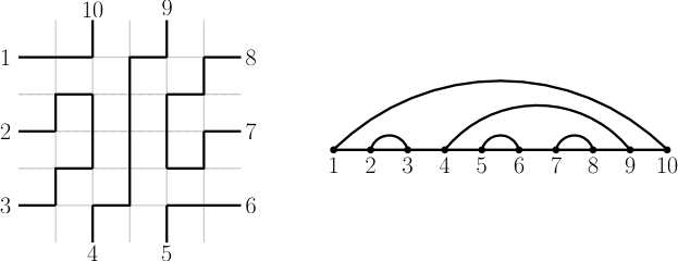
Figure 8. An example of an FPL of size $5$ and its link pattern.

It is well known that FPLs and alternating sign matrices (ASMs) are in bijection. The number of FPLs of size $n$, denoted by $\textnormal{ASM}(n)$, is hence given by the ASM-Theorem [9, 12]

$$\textnormal{ASM}(n)=\prod_{i=0}^{n-1}\frac{(3i+1)!}{(n+i)!}.$$

2.4. The (in-)homogeneous $O(\tau)$ loop model

A configuration of the inhomogeneous $O(\tau)$ loop model of size $n$ is a tiling of $[0,2n]\times[0,\infty)$ with plaquettes of side length $1$ depicted in Figure 9. To obtain a cylinder we identify the half-lines $\{(0,t),t\geq 0\}$ and $\{(2n,t),t\geq 0\}$. In the following we assume that the cylindrical loop percolations are filled randomly with the two plaquettes, where the probability to place the first plaquette of Figure 9 in column $i$ is $p_{i}$ with $0<p_{i}<1$ for all $1\leq i\leq 2n$. If the probability does not depend on the column, i. e., $p_{1}=\ldots=p_{2n}$, we call it the homogeneous $O(\tau)$ loop model. We parametrise the probabilities $p_{i}=\frac{qz_{i}-q^{-1}t}{qt-q^{-1}z_{i}}$ and $\tau=q+q^{-1}$. The two plaquettes in Figure 9 are interpreted to consist of two paths. By concatenating the paths of a plaquette with the paths of the neighbouring plaquettes, we see that a cylindrical loop percolation consists of noncrossing paths.

Figure 9. The two different plaquettes.

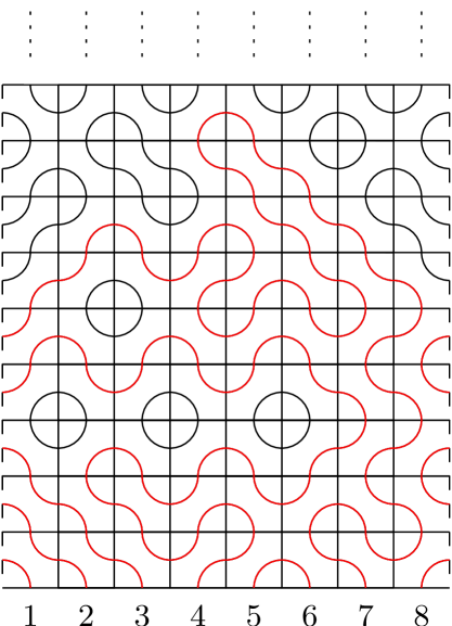
Figure 10. The beginning of a cylindrical loop percolation, where the paths starting and ending at the bottom are drawn in red.

Lemma 3.

With probability $1$ all paths in a random cylindrical loop percolation are finite.

A proof for the homogeneous case can be found in [11, Lemma 1.6], the inhomogeneous case can be proven analogously. For a configuration $C$ of the $O(\tau)$ loop model, we label the points $(i-\frac{1}{2},0)$ with $i$ for $1\leq i\leq 2n$. We define the connectivity pattern $\pi(C)$ as the noncrossing matching connecting $i$ and $j$ by an arch iff $i$ and $j$ are connected by paths in $C$. By the above lemma $\pi(C)$ is well defined for almost all cylindrical loop percolations $C$. For $\pi\in\textnormal{NC}_{n}$ denote by $\hat{\Psi}_{\pi}(t;z_{1},\ldots,z_{2n})$ the probability that a configuration $C$ has the connectivity pattern $\pi$ and write $\hat{\Psi}_{n}(t;z_{1},\ldots,z_{2n})=(\hat{\Psi}_{\pi}(t;z_{1},\ldots,z_{2n}))_{\pi\in\textnormal{NC}_{n}}$.

Figure 11. An example for a state transition starting with the noncrossing matching $\pi$ of Figure 1. The transition probability is $p_{1}(1-p_{2})(1-p_{3})p_{4}p_{5}(1-p_{6})$.

We define a Markov chain on the set $\textnormal{NC}_{n}$ of noncrossing matchings of size $n$. The transitions are given by putting $2n$ plaquettes below a noncrossing matching and simplify the paths to obtain a new noncrossing matching. An example is given in Figure 11. The probability of one transition is given by the product of the probabilities of placing the plaquettes, where placing the first plaquette of Figure 9 at the $i$-th position is $p_{i}$ as before. We denote by $T_{n}(t;z_{1},\ldots,z_{2n})$ the transition matrix of this Markov chain. By the Perron-Frobenius Theorem the matrix $T_{n}(t;z_{1},\ldots,z_{2n})$ has $1$ as an eigenvalue and the stationary distribution of the Markov chain is up to scaling the unique eigenvector with associated eigenvalue $1$. Every configuration $C$ of the inhomogeneous $O(\tau)$ loop model can be obtained uniquely by pushing all the plaquettes of a configuration $C^{\prime}$ one row up and filling the empty bottom row with plaquettes. Therefore the vector $\hat{\Psi}_{n}(t;z_{1},\ldots,z_{2n})$ is the stationary distribution of this Markov chain and hence satisfies

$$T_{n}(t;z_{1},\ldots,z_{2n})\hat{\Psi}_{n}(t;z_{1},\ldots,z_{2n})=\hat{\Psi}_{n}(t;z_{1},\ldots,z_{2n}).$$ (1)

We define the Hamiltonian as the linear map $\mathcal{H}_{n}:=\sum_{j=1}^{2n}e_{j}$, where $e_{j}$ is interpreted as an element of the Temperley-Lieb algebra.

Theorem 4.

The stationary distribution $\hat{\Psi}_{n}(t)=\hat{\Psi}_{n}(t;1,\ldots,1)$ satisfies for $\tau=1$

$$\mathcal{H}_{n}(\hat{\Psi}_{n}(t))=2n\hat{\Psi}_{n}(t).$$ (2)

Further $\hat{\Psi}_{n}(t)$ is independent of $t$ and uniquely determined by (2).

A proof of this theorem can be found for example in [11, Appendix B], however note that the matrix $H_{n}$ defined there is given by $2n\cdot\textnormal{Id}-\mathcal{H}_{n}$.

The following theorem was conjectured by Razumov and Stroganov in [10] and later proven by Cantini and Sportiello in [3]. It creates a connection between fully packed loop configurations and the stationary distribution of the homogeneous $O(1)$ loop model.

Theorem 5 (Razumov-Stroganov-Cantini-Sportiello Theorem).

Let $n\in\mathbb{N}$, set $q=e^{\frac{2\pi i}{3}}$ and $\hat{\Psi}_{\pi}=\hat{\Psi}_{\pi}(-q;1,\ldots,1)$. For all $\pi\in\textnormal{NC}_{n}$ holds

$$\hat{\Psi}_{\pi}=\frac{A_{\pi}}{\textnormal{ASM}(n)}.$$

3. The vector space $W_{n}[z]$

3.1. The quantum Knizhnik-Zamolodchikov equations

In order to introduce the quantum Knizhnik-Zamolodchikov equations (qKZ-equations), we need to define first the $R$-matrix and the operator $S_{i}$

$$\check{R}_{i}(u) =\frac{(qu-q^{-1})\textnormal{Id}+(u-1)e_{i}}{q-q^{-1}u},$$

$$S_{i}(z_{1},\ldots,z_{2n}) =\prod_{k=1}^{i-1}\check{R}_{i-k}\left(\frac{z_{i-k}}{q^{6}z_{i}}\right)\rho\prod_{k=1}^{2n-i}\check{R}_{2n-k}\left(\frac{z_{2n-k+1}}{z_{i}}\right),$$

for $1\leq i\leq 2n$, where $e_{i}$ is understood as an element of the Temperley-Lieb algebra and $\rho$ is the rotation as defined in section 2.2. Denote by $\Psi_{n}=(\Psi_{\pi})_{\pi\in\textnormal{NC}_{n}}$ a function in $z_{1},\ldots,z_{2n},q$. The level $1$ qKZ-equations are a system of $2n$ equations

$$S_{i}(z_{1},\ldots,z_{2n})\Psi_{n}(t;z_{1},\ldots,z_{2n})=\Psi_{n}(t;z_{1},\ldots,q^{6}z_{i},\ldots,z_{2n}),$$ (3)

with $1\leq i\leq 2n$. In the following we need the $2n+1$ equations

$$\check{R}_{i}\left(\frac{z_{i+1}}{z_{i}}\right)\Psi_{n}(t;z_{1},\ldots,z_{2n}) =\Psi_{n}(t;z_{1},\ldots,z_{i+1},z_{i},\ldots,z_{2n}),$$ (4a)

$$\rho^{-1}\Psi_{n}(t;z_{1},\ldots,z_{2n}) =\Psi_{n}(t;z_{2},\ldots,z_{2n},q^{6}z_{1}),$$ (4b)

where $1\leq i\leq 2n$ in (4a).

Proposition 6 ([13, section 4.1 and 4.3]).

1. The system of equations (4a) and (4b) imply the system of equations (3).

2. For $q=e^{\frac{2\pi i}{3}}$ and hence $\tau=1$, it holds $S_{i}(z_{1},\ldots,z_{2n})=T_{n}(z_{i};z_{1},\ldots,z_{2n})$. By using Lagrange interpolation one can show that (3) imply (1). Since the solutions of (1) form a one dimensional vector space, the same is true for solutions of the system of equations (3) for $q=e^{\frac{2\pi i}{3}}$.

3.2. Wheel polynomials

It turns out [5, Theorem 4] that for $q=e^{\frac{2\pi i}{3}}$ the components $\hat{\Psi}_{\pi}(t;z_{1},\ldots,z_{2n})$ of the stationary distribution of the inhomogeneous $O(1)$ loop model are up to a common factor homogeneous polynomials in $z_{1},\ldots,z_{2n}$ of degree $n(n-1)$ which are independent of $t$. In this section we characterise these homogeneous polynomials. In fact we characterise homogeneous solutions of degree $n(n-1)$ of (4a) and (4b) which are by Proposition 6 for $q=e^{\frac{2\pi i}{3}}$ also solutions of (1) . The results presented here can be found in [5, 6, 7, 13, 14] and [11].

Definition 7.

Let $n$ be a positive integer and $q$ a variable. A homogeneous polynomial $p\in\mathbb{Q}(q)[z_{1},\ldots,z_{2n}]$ of degree $n(n-1)$ is called wheel polynomial of order $n$ if it satisfies the wheel condition:

$$p(z_{1},\ldots,z_{2n})|_{q^{4}z_{i}=q^{2}z_{j}=z_{k}}=0,$$ (5)

for all triples $1\leq i<j<k\leq 2n$. Denote by $W_{n}[z]$ the $\mathbb{Q}(q)$-vector space of wheel polynomials of order $n$.

Theorem 8 ([6, Section 4.2]).

The dual space $W_{n}[z]^{*}$ of $W_{n}[z]$ is given by

$$W_{n}[z]^{*}=\bigoplus_{\pi\in\textnormal{NC}_{n}}\mathbb{Q}(q)\textnormal{ev}_{\pi},$$

where $\textnormal{ev}_{\pi}$ is defined as $\textnormal{ev}_{\pi}:p(z_{1},\ldots,z_{2n})\mapsto p(q^{\epsilon_{1}(\pi)},\ldots,q^{\epsilon_{2n}(\pi)})$ with $\epsilon_{i}(\pi)=-1$ iff an arch of $\pi$ has a left-endpoint labelled with $i$ and $\epsilon_{i}(\pi)=1$ otherwise.

Define the linear maps $\mathbf{S}_{k},\mathbf{D}_{k}:\mathbb{Q}(q)[z_{1},\ldots,z_{2n}]\rightarrow\mathbb{Q}(q)[z_{1},\ldots,z_{2n}]$ for $1\leq k\leq 2n$ as

$$\mathbf{S}_{k}:\quad f(z_{1},\ldots,z_{2n})\;\mapsto\;f(z_{1},\ldots,z_{k+1},z_{k},\ldots,z_{2n}),$$ (6)

$$\mathbf{D}_{k}:\quad f\;\mapsto\;\frac{qz_{k}-q^{-1}z_{k+1}}{z_{k+1}-z_{k}}(\mathbf{S}_{k}(f)-f).$$ (7)

By setting $\mathbf{D}_{k+2n}:=\mathbf{D}_{k}$ we extend the definition of $\mathbf{D}_{k}$ to all integers $k$.
The operators $\mathbf{D}_{k}$ are introduced as an abbreviation for $(qz_{k}-q^{-1}z_{k+1})\delta_{k}$, where $\delta_{k}=\frac{1}{z_{k+1}-z_{k}}(\mathbf{S}_{k}-\textnormal{Id})$ has been used before , e. g., in [13]. One can verify easily the following Lemma.

Lemma 9.

1. The space $W_{n}[z]$ of all wheel polynomials of order $n$ is closed under the action of $\mathbf{D}_{k}$ for $1\leq k\leq 2n-1$. If $q=e^{\frac{2\pi i}{3}}$ the vector space $W_{n}[z]$ is also closed under $\mathbf{D}_{2n}$.

2. For all $1\leq k\leq 2n$ and all polynomials $f,g\in\mathbb{Q}(q)[z_{1},\ldots,z_{2n}]$ one has

   $$\mathbf{D}_{k}(fg)=\mathbf{D}_{k}(f)\mathbf{S}_{k}(g)+f\mathbf{D}_{k}(g).$$ (8)

The following theorem describes a very important $\mathbb{Q}(q)$-basis of $W_{n}[z]$.

Theorem 10 ([13, Section 4.2]).

Set

$$\Psi_{()_{n}}(z_{1},\ldots,z_{2n}):=(q-q^{-1})^{-n(n-1)}\prod_{1\leq i<j\leq n}(qz_{i}-q^{-1}z_{j})(qz_{n+i}-q^{-1}z_{n+j}).$$ (9)

Define for two noncrossing matchings $\sigma,\pi$ with $\sigma\nearrow_{j}\pi$

$$\Psi_{\pi}:=\mathbf{D}_{j}(\Psi_{\sigma})-\sum_{\tau\in e_{j}^{-1}(\sigma)\setminus\{\sigma,\pi\}}\Psi_{\tau}.$$ (10)

Then $\Psi_{\pi}$ is well-defined for all $\pi\in\textnormal{NC}_{n}$ and satisfies

$$\Psi_{\rho^{-1}(\pi)}(z_{1},\ldots,z_{2n})=\Psi_{\pi}(z_{2},\ldots,z_{2n},q^{6}z_{1}).$$ (11)

The set $\{\Psi_{\pi},\pi\in\textnormal{NC}_{n}\}$ is further a $\mathbb{Q}(q)$-basis of $W_{n}[z]$.

The noncrossing matchings $\tau$ which appear in the sum of (10) satisfy by Lemma 2 the relation $\tau<\pi$. Hence we can use (10) to calculate the basis $\Psi_{\pi}$ of $W_{n}[z]$ recursively. The vector $\Psi_{n}=(\Psi_{\pi})_{\pi\in\textnormal{NC}_{n}}$ satisfies (4a). This is true since we can reformulate (4a) as

$$e_{i}\Psi_{n}=\mathbf{D}_{i}(\Psi_{n})-(q+q^{-1})\Psi_{n},$$ (12)

for $1\leq i\leq 2n-1$. Let $\sigma,\pi\in\textnormal{NC}_{n}$ with $\sigma\nearrow_{i}\pi$, then the $\sigma$ component of both sides in (12) is

$$\Psi_{\pi}-(q+q^{-1})\Psi_{\sigma}+\sum_{\tau\in e_{i}^{-1}(\sigma)\setminus\{\sigma,\pi\}}\Psi_{\tau}=\mathbf{D}_{i}(\Psi_{\sigma})-(q+q^{-1})\Psi_{\sigma},$$

which is exactly (10). Since $\Psi_{n}$ satisfies (4b) by Theorem 10, Proposition 6 states that $\Psi_{n}$ is a solution of the qKZ equations and therefore for $\tau=1$ a multiple of the stationary distribution of the inhomogeneous $O(1)$ loop model. By setting $z_{1}=\ldots=z_{2n}=1$ Theorem 5 implies $\Psi_{\pi}(1,\ldots,1)|_{\tau=1}=cA_{\pi}$ for an appropriate constant $c$. Because of $\Psi_{()_{n}}(1,\ldots,1)|_{\tau=1}=1=A_{()_{n}}$ by definition, and Theorem 5 we obtain the following theorem.

Theorem 11.

Set $q=e^{\frac{2\pi i}{3}}$ and let $\pi\in\textnormal{NC}_{n}$, then one has

$$\Psi_{\pi}(z_{1},\ldots,z_{2n}) =\textnormal{ASM}(n)\times\hat{\Psi}_{n}(t;z_{1},\ldots,z_{2n}),$$

$$\Psi_{\pi}(1,\ldots,1) =A_{\pi}.$$

3.3. A new basis for $W_{n}[z]$

The following lemma is a direct consequence of the definitions of the $\mathbf{D}_{i}$’s and $\Psi_{()_{n}}$.

Lemma 12.

Let $n$ be a positive integer, then one has

1. $\mathbf{D}_{i}\circ\mathbf{D}_{i}=(q+q^{-1})\mathbf{D}_{i}$ for $1\leq i\leq 2n$,

2. $\mathbf{D}_{i}\circ\mathbf{D}_{j}=\mathbf{D}_{j}\circ\mathbf{D}_{i}$ for $1\leq i,j\leq 2n$ with $|i-j|>1$,

3. $\mathbf{D}_{i+1}\circ\mathbf{D}_{i}\circ\mathbf{D}_{i+1}+\mathbf{D}_{i}=\mathbf{D}_{i}\circ\mathbf{D}_{i+1}\circ\mathbf{D}_{i}+\mathbf{D}_{i+1}$ for $1\leq i\leq 2n$,

4. $\mathbf{D}_{i}(\Psi_{()_{n}})=(q+q^{-1})\Psi_{()_{n}}$ for $i\notin\{n,2n\}$.

In the following we write $\prod_{i=1}^{n}\mathbf{D}_{i}$ for the product $\mathbf{D}_{1}\circ\ldots\circ\mathbf{D}_{n}$. Let $\pi$ be a noncrossing matching with corresponding Young diagram $\lambda(\pi)=(\lambda_{1},\ldots,\lambda_{l})$, i. e., $\lambda_{i}$ is the number of boxes of $\lambda(\pi)$ in the $i$-th row from top. We define the wheel polynomial $D_{\pi}$ by the following algorithm. First write in every box of $\lambda(\pi)$ the number of the diagonal the box lies on. The wheel polynomial $D_{\pi}$ is then constructed recursively by “reading” in the Young diagram $\lambda(\pi)$ the rows from top to bottom and in the rows all boxes from left to right and apply $\mathbf{D}_{\textit{number in the box}}$ to the previous wheel polynomial, starting with $\Psi_{()_{n}}$, which is defined in (9). For $\pi$ as in Figure 12 we obtain

$$D_{\pi}=\left(\mathbf{D}_{n-3}\circ\mathbf{D}_{n-2}\circ\mathbf{D}_{n}\circ\mathbf{D}_{n-1}\circ\mathbf{D}_{n+3}\circ\mathbf{D}_{n+2}\circ\mathbf{D}_{n+1}\circ\mathbf{D}_{n}\right)(\Psi_{()_{n}}).$$

Alternatively we can write $D_{\pi}$ directly as

$$D_{\pi}=\left(\prod_{i=1}^{l}\prod_{j=1}^{\lambda_{l+1-i}}\mathbf{D}_{n+(i-l)+(\lambda_{l+1-i}-j)}\right)(\Psi_{()_{n}}).$$ (13)

Figure 12. The numbers indicate the labels of the diagonals the boxes lie on.

Theorem 13.

The set of wheel polynomials $\{D_{\pi}|\pi\in\textnormal{NC}_{n}\}$ is a $\mathbb{Q}(q)$-basis of $W_{n}[z]$. Further $\Psi_{\pi}$ is for $\pi\in\textnormal{NC}_{n}$ a linear combination of $D_{\tau}$’s with $\tau\leq\pi$ and the coefficient of $D_{\pi}$ is $1$.

Proof.

We prove the second statement by induction on the number of boxes of $\lambda(\pi)$. It is by definition true for $()_{n}$, hence let the number $|\lambda(\pi)|$ be non-zero. Let $\sigma$ be the noncrossing matching such that $\lambda(\sigma)$ is the Young diagram one obtains by deleting the rightmost box in the bottom row of $\lambda(\pi)$, and let $i$ be the integer such that $\sigma\nearrow_{i}\pi$. Then Theorem 10 states

$$\Psi_{\pi}=\mathbf{D}_{i}\Psi_{\sigma}-\sum_{\tau\in e_{i}^{-1}(\sigma)\setminus\{\sigma,\pi\}}\Psi_{\tau}.$$

We use the induction hypothesis to express $\Psi_{\tau}$ and $\Psi_{\sigma}$ as sums of $D_{\tau^{\prime}}$ with $\tau^{\prime}\leq\tau<\pi$ or $D_{\sigma^{\prime}}$ with $\sigma^{\prime}\leq\sigma<\pi$ respectively. The coefficient of $D_{\sigma}$ in $\Psi_{\sigma}$ is by the induction hypothesis equals to $1$. Since all $\sigma^{\prime}\leq\sigma$ satisfy the requirements of Lemma 14, this lemma implies the statement. By above arguments the set $\{D_{\pi}|\pi\in\textnormal{NC}_{n}\}$ is a $\mathbb{Q}(q)$-generating set for $W_{n}[z]$ of cardinality $\dim_{\mathbb{Q}(q)}(W_{n}[z])$, hence it is also a $\mathbb{Q}(q)$-basis. ∎

The next lemma contains the technicalities which are needed to prove the above theorem.

Lemma 14.

Let $1<i<2n$ and $\sigma\in\textnormal{NC}_{n}$ such that the number of boxes on the $i$-th diagonal of $\lambda(\sigma)$ is less than the maximal possible number of boxes that can be placed there. Then $\mathbf{D}_{i}(D_{\sigma})=D_{\pi}$ iff there exists a $\pi\in\textnormal{NC}_{n}$ with $\sigma\nearrow_{i}\pi$ or otherwise $\mathbf{D}_{i}(D_{\sigma})$ is a $\mathbb{Q}(q)$-linear combination of $D_{\tau}$’s with $\tau\leq\sigma$.

Proof.

We use induction on the number of boxes of $\lambda(\sigma)$. We say that $i$ appears in $\sigma$ if there is a box in $\lambda(\sigma)$ which lies on the $i$-th diagonal.

1. Assume that $i$ does not appear in $\sigma$. This implies that $i-1$ can not appear in $\sigma$. Then there are two cases:

   1. First $i+1$ does not appear in $\sigma$. By Lemma 12 $\mathbf{D}_{i}$ commutes with all the $\mathbf{D}$-operators appearing in $D_{\sigma}$. If $i\neq n$ Lemma 12 states $\mathbf{D}_{i}(\Psi_{()_{n}})=(q+q^{-1})\Psi_{()_{n}}$ and hence $\mathbf{D}_{i}(D_{\sigma})=(q+q^{-1})D_{\sigma}$. The case $i=n$ implies $\sigma=()_{n}$ and hence $\mathbf{D}_{i}(D_{\sigma})=D_{(()())_{n-2}}$.

   2. In the second case $i+1$ appears in $\sigma$. Then there is only one box on the $(i+1)$-th diagonal. This box is the leftmost box of the bottom row of $\lambda(\sigma)$. Let $\pi$ be the noncrossing matching whose corresponding Young diagram is obtained by adding a box in a new row in $\lambda(\sigma)$, i. e., $\sigma\nearrow_{i}\pi$. By definition holds $D_{\pi}=\mathbf{D}_{i}(D_{\sigma})$.

2. Let $i$ appear in $\sigma$. We consider the lowest box in the $i$-th diagonal and call it $X$. Let $\sigma^{\prime}$ be the noncrossing matching of size $n$ whose corresponding Young diagram $\lambda(\sigma^{\prime})$ consists of all boxes above and to the left of the box $X$, denote by $\alpha_{i}$ with $1\leq i\leq A$ the boxes to the right of $X$ and in the row below but excluding the boxes in the $(i+1)$-th and $(i-1)$-th diagonal and by $\beta_{i}$ with $1\leq i\leq B$ the remaining boxes at the bottom. A schematic picture is given in Figure 13. Using the previous definitions we can write $D_{\sigma}$ as

   $$D_{\sigma}=\left(\prod_{l=1}^{B}\mathbf{D}_{\beta_{l}}\circ\mathbf{D}_{i-1}^{b}\circ\prod_{l=1}^{A}\mathbf{D}_{\alpha_{l}}\circ\mathbf{D}_{i+1}^{a}\circ\mathbf{D}_{i}\right)(D_{\sigma^{\prime}}),$$ (14)

   where $a,b$ are $0$ or $1$.

   

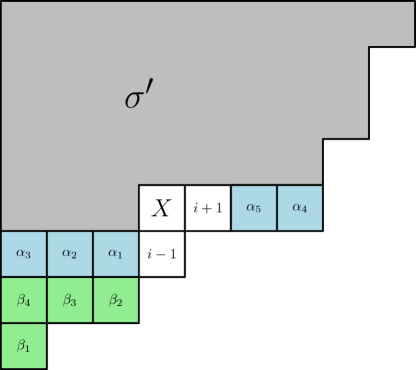
   Figure 13. Schematic representation of $\lambda(\sigma)$ for $\sigma$ as in the second case of the proof of Lemma 14 with $a=b=1$.

   1. If $a=b=0$ Lemma 12 (1,2) implies

      $$\mathbf{D}_{i}D_{\sigma} =\mathbf{D}_{i}\left(\prod_{l=1}^{B}\mathbf{D}_{\beta_{l}}\circ\prod_{l=1}^{A}\mathbf{D}_{\alpha_{l}}\circ\mathbf{D}_{i}\right)(D_{\sigma^{\prime}})$$

      $$=\left(\prod_{l=1}^{B}\mathbf{D}_{\beta_{l}}\circ\prod_{l=1}^{A}\mathbf{D}_{\alpha_{l}}\circ\mathbf{D}_{i}^{2}\right)(D_{\sigma^{\prime}})$$

      $$=\left(\prod_{l=1}^{B}\mathbf{D}_{\beta_{l}}\circ\prod_{l=1}^{A}\mathbf{D}_{\alpha_{l}}\circ((q+q^{-1})\mathbf{D}_{i})\right)(D_{\sigma^{\prime}})=(q+q^{-1})D_{\sigma}.$$

   2. For $a=b=1$, the operator $\mathbf{D}_{i}$ commutes with all $\mathbf{D}_{\beta_{l}}$. As Figure 13 shows and by the assumptions on $\sigma$ there exists a noncrossing matching $\pi$ with $\sigma\nearrow_{i}\pi$. Hence one has

      $$\mathbf{D}_{i}(D_{\sigma})=\left(\prod_{l=1}^{B}\mathbf{D}_{\beta_{l}}\circ\mathbf{D}_{i}\circ\mathbf{D}_{i-1}\circ\prod_{l=1}^{A}\mathbf{D}_{\alpha_{l}}\circ\mathbf{D}_{i+1}\circ\mathbf{D}_{i}\right)(D_{\sigma^{\prime}})=D_{\pi}.$$

   3. For $a=1,b=0$ we obtain by Lemma 12 (2,3)

      $$\mathbf{D}_{i}(D_{\sigma}) =\left(\prod_{l=1}^{B}\mathbf{D}_{\beta_{l}}\circ\prod_{l=1}^{A}\mathbf{D}_{\alpha_{l}}\circ\mathbf{D}_{i}\circ\mathbf{D}_{i+1}\circ\mathbf{D}_{i}\right)(D_{\sigma^{\prime}})$$

      $$=\left(\prod_{l=1}^{B}\mathbf{D}_{\beta_{l}}\circ\prod_{l=1}^{A}\mathbf{D}_{\alpha_{l}}\right)\left((\mathbf{D}_{i+1}\circ\mathbf{D}_{i}\circ\mathbf{D}_{i+1}+\mathbf{D}_{i}-\mathbf{D}_{i+1})(D_{\sigma^{\prime}})\right).$$

      By the induction hypothesis $\left((\mathbf{D}_{i+1}\circ\mathbf{D}_{i}\circ\mathbf{D}_{i+1}+\mathbf{D}_{i}-\mathbf{D}_{i+1})(D_{\sigma^{\prime}})\right)$ is a linear combination of $D_{\tau}$’s with $\tau\leq\hat{\sigma}$ where $\hat{\sigma}$ is $\sigma^{\prime}$ with a box added on the $i$-th and $i+1$-th diagonal. Using again the induction hypothesis for the $D_{\tau}$’s with $\tau\leq\hat{\sigma}$ proofs the claim.

   4. Let $a=0,b=1$ and let $\hat{\sigma}$ be the noncrossing matching whose Young diagram consists of $\lambda(\sigma^{\prime})$ and the boxes labelled with $\alpha_{i}$ for $1\leq i\leq A$. Lemma 12 (2,3) implies

      $$\mathbf{D}_{i}(D_{\sigma}) =\left(\prod_{l=1}^{B}\mathbf{D}_{\beta_{l}}\circ\mathbf{D}_{i}\circ\mathbf{D}_{i-1}\circ\mathbf{D}_{i}\circ\prod_{l=1}^{A}\mathbf{D}_{\alpha_{l}}\right)(D_{\sigma^{\prime}})$$

      $$=\left(\prod_{l=1}^{B}\mathbf{D}_{\beta_{l}}\circ(\mathbf{D}_{i-1}\circ\mathbf{D}_{i}\circ\mathbf{D}_{i-1}+\mathbf{D}_{i}-\mathbf{D}_{i-1})\right)(D_{\hat{\sigma}}).$$

      We finish the proof by using the induction hypothesis analogously to the above case. ∎

Let $\pi\in\textnormal{NC}_{n}$ be a noncrossing matching given by $\pi=\pi_{1}\pi_{2}$ where $\pi_{i}$ is a noncrossing matching of size $n_{i}$ for $i=1,2$. We want to generalise $D_{\pi}$ and Theorem 13 in the sense that we can write $\Psi_{\pi}=\Psi_{\pi_{1}\pi_{2}}$ as a linear combination of $D_{\tau_{1},\tau_{2}}$ with $\tau_{i}\leq\pi_{i}$ for $i=1,2$. This will not be possible for $\Psi_{\pi}$ but for $\Psi_{\rho^{n_{2}}\pi}$. Let the Young diagram corresponding to $\pi_{2}$ be given as $\lambda(\pi_{2})=(\lambda_{1},\ldots,\lambda_{l})$. The wheel polynomial $D_{\pi_{1},\pi_{2}}$ is then defined by the following algorithm. First we write in every box of $\lambda(\pi_{2})$ the number of the diagonal the box lies on. The wheel polynomial $D_{\pi_{1}\pi_{2}}$ is then constructed recursively by “reading” in the Young diagram $\lambda(\pi_{2})$ the rows from top to bottom and in the rows all boxes from left to right and apply $\mathbf{D}_{\textit{number in the box}-n}$ to the previous wheel polynomial, starting with $D_{(\pi_{1})_{n_{2}}}$, which is defined in (13). Remember that we have extended the definition of $\mathbf{D}_{k}$ to all integers via $\mathbf{D}_{k}=\mathbf{D}_{k+2n}$. We can express $D_{\pi_{1},\pi_{2}}$ also by the following formula

$$D_{\pi_{1},\pi_{2}}:=\left(\prod_{i=1}^{l}\prod_{j=1}^{\lambda_{l+1-i}}\mathbf{D}_{(i-l)+(\lambda_{l+1-i}-j)}\right)(D_{(\pi_{1})_{n_{2}}}).$$

For $\pi_{2}$ as in Figure 12 we obtain

$$D_{\pi_{1},\pi_{2}}=\left(\mathbf{D}_{-3}\circ\mathbf{D}_{-2}\circ\mathbf{D}_{0}\circ\mathbf{D}_{-1}\circ\mathbf{D}_{3}\circ\mathbf{D}_{2}\circ\mathbf{D}_{1}\circ\mathbf{D}_{0}\right)(D_{(\pi_{1})_{n_{2}}}).$$

Theorem 15.

Let $\pi=\pi_{1}\pi_{2},\pi_{1},\pi_{2}$ be noncrossing matching of size $n,n_{1}$ or $n_{2}$ respectively and set $q=e^{\frac{2\pi i}{3}}$. The wheel polynomial

$$\Psi_{\rho^{n_{2}}(\pi_{1}\pi_{2})}(z_{1},\ldots,z_{2n})=\Psi_{\pi_{1}\pi_{2}}(z_{2n+1-n_{2}},\ldots,z_{2n},z_{1},\ldots,z_{2n-n_{2}})$$

can be expressed as a linear combination of $D_{\tau_{1},\tau_{2}}$’s where $\tau_{i}\leq\pi_{i}$ and the coefficient of $D_{\pi_{1},\pi_{2}}$ is $1$.

Proof.

We calculate $\Psi_{\rho^{n_{2}}(\pi_{1}\pi_{2})}$ in three steps:

1. $\Psi_{(\pi_{1})_{n_{2}}}$ is by Theorem 13 a linear combination of $D_{(\tau_{1})_{n_{2}}}$’s with $\tau_{1}\leq\pi_{1}$ and the coefficient of $D_{(\pi_{1})_{n_{2}}}$ is $1$.

2. Theorem 10 implies

   $$\Psi_{\pi_{1}()_{n_{2}}}=\Psi_{\rho^{-n_{2}}((\pi_{1})_{n_{2}})}=\Psi_{(\pi_{1})_{n_{2}}}(z_{n_{2}+1},\ldots,z_{2n},z_{1},\ldots,z_{n_{2}}).$$

3. Use the recursion (10) of Theorem 10 to obtain $\Psi_{\pi_{1}\pi_{2}}$ starting from $\Psi_{\pi_{1}()_{n_{2}}}$. By Lemma 2 the $\tau$ appearing in the sum in (10) are of the form $\pi_{1}\tau_{2}$ with $\tau_{2}\leq\pi_{2}$.

The algorithm for calculating $\Psi_{(\pi_{2})_{n_{1}}}$ and the third step of calculating $\Psi_{\pi_{1}\pi_{2}}$ differ by the initial condition – in the first case $\Psi_{()_{n}}$, in the second $\Psi_{\pi_{1}()_{n_{2}}}$ – and each $\mathbf{D}_{i}$ of the first algorithm is replaced by $\mathbf{D}_{i+n_{2}}$. Hence we can use Theorem 13 to express $\Psi_{\pi_{1}\pi_{2}}$ as a linear combination of $\hat{D}_{\tau_{2}}$ with $\tau_{2}\leq\pi_{2}$, where $\hat{D}_{(\tau_{2})_{n_{1}}}$ is obtained by taking $D_{(\tau_{2})_{n_{1}}}$ and changing every $\mathbf{D}_{i}$ to a $\mathbf{D}_{i+n_{2}}$ and $\Psi_{()_{n}}$ is replaced by $\Psi_{\pi_{1}()_{n_{2}}}$. Together with the first two parts of the algorithm this implies that $\Psi_{\rho^{n_{2}}(\pi_{1}\pi_{2})}$ is a linear combination of $D_{\tau_{1},\tau_{2}}$’s with $\tau_{i}\leq\pi_{i}$ and the coefficient of $D_{\pi_{1},\pi_{2}}$ is $1$. ∎

Remark 16.

Let $\Psi_{\pi_{i}}=\sum_{\tau_{i}\leq\pi_{i}}\alpha_{\tau_{i}}D_{\tau_{i}}$ for $i=1,2$. The above proof implies

$$\Psi_{\rho^{n_{2}}(\pi_{1}\pi_{2})}=\sum_{\tau_{1}\leq\pi_{1},\tau_{2}\leq\pi_{2}}\alpha_{\tau_{1}}\alpha_{\tau_{2}}D_{\tau_{1},\tau_{2}}.$$

Hence gaining knowledge about

$$A_{\pi_{1}\pi_{2}}=\Psi_{\pi_{1}\pi_{2}}|_{z_{1}=\ldots=z_{2n}=1,q^{3}=1}=\Psi_{\rho^{n_{2}}(\pi_{1}\pi_{2})}|_{z_{1}=\ldots=z_{2n}=1,q^{3}=1}$$

could be achieved by understanding the coefficients $\alpha_{\tau_{i}}$ and the behaviour of $D_{\tau_{1},\tau_{2}}$ for $\tau_{i}\leq\pi_{i}$. However this seems to be very difficult.

4. Fully packed loops with a set of nested arches

In order to prove Theorem 1 we will need to calculate $D_{\pi_{1},\pi_{2}}$ at $z_{1}=\ldots=z_{2(n_{1}+n_{2})}=1$ for two noncrossing matchings $\pi_{1},\pi_{2}$. The following notations will simplify this task. We define

$$f(i,j) :=\frac{qz_{i}-q^{-1}z_{j}}{q-q^{-1}},\quad g(i):=\frac{q-q^{-1}z_{i}}{q-q^{-1}},\quad h(i):=\frac{qz_{i}-q^{-1}}{q-q^{-1}},$$

for $1\leq i\neq j\leq 2n$. Using this notations we obtain

$$\Psi_{()_{n}}=\prod_{1\leq i<j\leq n}f(i,j)f(n+i,n+j).$$

One verifies the following lemma by simple calculation.

Lemma 17.

For $1\leq i,j,k\leq 2n$ and $i\neq j$ one has

1. $\mathbf{D}_{k}(f(i,j))=\begin{cases}(q+q^{-1})f(k,k+1)\quad&(i,j)=(k,k+1),\\ -(q+q^{-1})f(k,k+1)&(i,j)=(k+1,k),\\ qf(k,k+1)&i=k;\;j\neq k+1,\\ -qf(k,k+1)&i=k+1;\;j\neq k,\\ -q^{-1}f(k,k+1)&j=k;\;i\neq k+1,\\ q^{-1}f(k,k+1)&j=k+1;\;i\neq k,\\ 0&\{i,j\}\cap\{k,k+1\}=\emptyset,\end{cases}$

2. $\mathbf{D}_{k}(g(i))=\begin{cases}-q^{-1}f(k,k+1)&i=k,\\ q^{-1}f(k,k+1)\quad&i=k+1,\\ 0&\text{otherwise},\end{cases}$

3. $\mathbf{D}_{k}(h(i))=\begin{cases}qf(k,k+1)\quad&i=k,\\ -qf(k,k+1)&i=k+1,\\ 0&\text{otherwise}.\end{cases}$

4. Let $m$ be a positive integer, then the following holds

   $$\mathbf{D}_{k}(f(i,j)^{m}) =\mathbf{D}_{k}(f(i,j))\sum_{l=0}^{m-1}f(i,j)^{l}\mathbf{S}_{k}(f(i,j)^{m-1-l}),$$

   $$\mathbf{D}_{k}(g(i)^{m}) =\mathbf{D}_{k}(g(i))\sum_{l=0}^{m-1}g(i)^{l}\mathbf{S}_{k}(g(i)^{m-1-l}),$$

   $$\mathbf{D}_{k}(h(i)^{m}) =\mathbf{D}_{k}(h(i))\sum_{l=0}^{m-1}h(i)^{l}\mathbf{S}_{k}(h(i)^{m-1-l}).$$

We further introduce the abbreviation

$$P(\alpha_{i,j}|\beta_{i}|\gamma_{i}):=\prod_{1\leq i\neq j\leq 2n}f(i,j)^{\alpha_{i,j}}\prod_{i=1}^{2n}g(i)^{\beta_{i}}h(i)^{\gamma_{i}},$$

where $\alpha_{i,j},\beta_{i},\gamma_{i}$ are nonnegative integers for $1\leq i\neq j\leq 2n$. Our goal is to obtain a useful expression for $\mathbf{D}_{i_{1}}\circ\cdots\circ\mathbf{D}_{i_{m}}(P(\alpha_{i,j}|\beta_{i}|\gamma_{i}))|_{z_{1}=\ldots=z_{2n}=1}$ for special values of $\alpha_{i,j},\beta_{i}$ and $\gamma_{i}$. By using the previous lemma it is very easy to see that $\mathbf{D}_{i_{1}}\circ\cdots\circ\mathbf{D}_{i_{m}}(P(\alpha_{i,j}|\beta_{i}|\gamma_{i}))$ is a sum of products of the form $P(\alpha^{\prime}_{i,j}|\beta^{\prime}_{i}|\gamma^{\prime}_{i})$. The explicit form of this sum is easy to understand when only one $\mathbf{D}$-operator is applied but gets very complicated for more. However it turns out that $\mathbf{D}_{i_{1}}\circ\cdots\circ\mathbf{D}_{i_{m}}(P(\alpha_{i,j}|\beta_{i}|\gamma_{i}))|_{z_{1}=\ldots=z_{2n}=1}$ is a polynomial in $\alpha_{i,j},\beta_{i}$ and $\gamma_{i}$, which is stated in Lemma 19. The next example hints at the basic idea behind this fact.

Example 18.

Let $P=P(\alpha_{i,j}|\beta_{i}|\gamma_{i})$ and $n=1$. We calculate $\mathbf{D}_{1}(P)_{z_{1}=z_{2}=1}$ explicitly. By using Lemma 9 and Lemma 17 we obtain for $\mathbf{D}_{1}(P)$ the expression.

$$\mathbf{D}_{1}(P)= \mathbf{D}_{1}\left(f(1,2)^{\alpha_{1,2}}f(2,1)^{\alpha_{2,1}}g(1)^{\beta_{1}}g(2)^{\beta_{2}}h(1)^{\gamma_{1}}h(2)^{\gamma_{2}}\right)$$

$$= (q+q^{-1})\sum_{t=0}^{\alpha_{1,2}-1}f(1,2)^{\alpha_{1,2}+\alpha_{2,1}-t}f(2,1)^{t}g(1)^{\beta_{2}}g(2)^{\beta_{1}}h(1)^{\gamma_{2}}h(2)^{\gamma_{1}}+$$

$$-(q+q^{-1})\sum_{t=0}^{\alpha_{2,1}-1}f(1,2)^{\alpha_{1,2}+\alpha_{2,1}-t}f(2,1)^{t}g(1)^{\beta_{2}}g(2)^{\beta_{1}}h(1)^{\gamma_{2}}h(2)^{\gamma_{1}}+$$

$$-q^{-1}\sum_{t=0}^{\beta_{1}-1}f(1,2)^{\alpha_{1,2}+1}f(2,1)^{\alpha_{2,1}}g(1)^{\beta_{1}+\beta_{2}-t-1}g(2)^{t}h(1)^{\gamma_{2}}h(2)^{\gamma_{1}}+$$

$$+q^{-1}\sum_{t=0}^{\beta_{2}-1}f(1,2)^{\alpha_{1,2}+1}f(2,1)^{\alpha_{2,1}}g(1)^{\beta_{1}+\beta_{2}-t-1}g(2)^{t}h(1)^{\gamma_{2}}h(2)^{\gamma_{1}}+$$

$$+q\sum_{t=0}^{\gamma_{1}-1}f(1,2)^{\alpha_{1,2}+1}f(2,1)^{\alpha_{2,1}}g(1)^{\beta_{1}}g(2)^{\beta_{2}}h(1)^{\gamma_{1}+\gamma_{2}-t-1}h(2)^{t}+$$

$$-q\sum_{t=0}^{\gamma_{2}-1}f(1,2)^{\alpha_{1,2}+1}f(2,1)^{\alpha_{2,1}}g(1)^{\beta_{1}}g(2)^{\beta_{2}}h(1)^{\gamma_{1}+\gamma_{2}-t-1}h(2)^{t}.$$

By evaluating this at $z_{1}=z_{2}=1$ we obtain:

$$\mathbf{D}_{1}(P)|_{z_{1}=z_{2}=1}=(q+q^{-1})(\alpha_{1,2}-\alpha_{2,1})+q^{-1}(\beta_{2}-\beta_{1})+q(\gamma_{1}-\gamma_{2}),$$

which is a polynomial in the $\alpha_{i,j},\beta_{i},\gamma_{i}$.

The proof of Theorem 1 is achieved by using two main ingredients. First Theorem 15 allows us to express the wheel polynomial $\Psi_{(\pi_{1})_{m}\pi_{2}}$ in a suitable basis and second Lemma 19 tells us what we have to expect when evaluating the basis at $z_{1}=\ldots=z_{2N}=1$.

Proof of Theorem 1.

In the following we show that the number $A_{(\pi_{1})_{m}\pi_{2}}$ of FPLs with link pattern $(\pi_{1})_{m}\pi_{2}$ is a polynomial in $m$. Together with [4, Theorem $6.7$], which states that $A_{(\pi_{1})_{m}\pi_{2}}$ is a polynomial in $m$ with requested degree and leading coefficient for large values of $m$, this proves Theorem 1.

Set $N=m+n_{1}+n_{2}$ and $q=e^{\frac{2\pi i}{3}}$. By Theorem 11, Theorem 5 and Theorem 10 one has

$$A_{(\pi_{1})_{m}\pi_{2}}=\Psi_{(\pi_{1})_{m}\pi_{2}}|_{z_{1}=\ldots=z_{2N}=1}=\Psi_{\rho^{n_{2}}((\pi_{1})_{m}\pi_{2})}|_{z_{1}=\ldots=z_{2N}=1}.$$

Theorem 15 implies that $\Psi_{\rho^{n_{2}}((\pi_{1})_{m}\pi_{2})}$ is a linear combination of $D_{(\tau_{1})_{m},\tau_{2}}$ with $\tau_{i}\leq\pi_{i}$ for $i=1,2$. By definition $D_{(\tau_{1})_{m},\tau_{2}}$ is of the form $\prod_{j=1}^{k}\mathbf{D}_{i_{j}}(\Psi_{()_{N}})$ with $k\leq|\lambda(\pi_{1})|+|\lambda(\pi_{2})|$ and $i_{j}\in\{1,\ldots,n_{2}-2,N-n_{1}+2,\ldots,N+n_{1}-2,2N-n_{2}+2,\ldots,2N\}$ for $1\leq j\leq k$. The operator $\mathbf{D}_{i_{j}}$ acts for $1\leq j\leq k$ trivially on $z_{i}$ with $i\in I:=\{n_{2}+1,\ldots,N-n_{1},N+n_{1}+1,\ldots,2N-n_{2}\}$. Hence one has

$$\left.\left(\prod_{j=1}^{k}\mathbf{D}_{i_{j}}(\Psi_{()_{N}})\right)\right|_{z_{1}=\ldots=z_{2N}=1}=\left.\left(\prod_{j=1}^{k}\mathbf{D}_{i_{j}}(\Psi_{()_{N}|\forall i\in I:z_{i}=1})\right)\right|_{\forall i\in\{1,\ldots,2N\}\setminus I:z_{i}=1}.$$

The polynomial $\left.\Psi_{()_{N}}\right|_{z_{i}=1\forall i\in I}$ is a polynomial in the $2(n_{1}+n_{2})$ variables $z_{i}$, where $i$ is an element of $\{1,\ldots,2N\}\setminus I$. For simplicity we substitute these remaining variables with $z_{1},\ldots,z_{2(n_{1}+n_{2})}$ whereby we keep the same order on the indices. Hence $\left.\Psi_{()_{N}}\right|_{z_{i}=1\forall i\in I}$ can be written in the form $P=P(\alpha_{i,j}|\beta_{i}|\gamma_{i})$ with

$$\alpha_{i,j} =\begin{cases}1\quad&i<j\textit{ and }\left(j\leq n_{1}+n_{2}\text{ or }i>n_{1}+n_{2}\right),\\ 0&\text{otherwise},\end{cases}$$

$$\beta_{i} =\begin{cases}m\quad&i\in\{n_{2}+1,\ldots,n_{1}+n_{2},2n_{1}+n_{2}+1,\ldots,2(n_{1}+n_{2})\},\\ 0&\text{otherwise},\end{cases}$$

$$\gamma_{i} =\begin{cases}m\quad&i\in\{1,\ldots,n_{2},n_{1}+n_{2}+1,\ldots,2n_{1}+n_{2}\},\\ 0&\text{otherwise},\end{cases}$$

whereas all the $z_{i}$ in $f(i,j),g(i)$ and $h(i)$ are replaced by $\hat{z}_{i}$. Lemma 19 implies that $\prod_{j=1}^{k}\mathbf{D}_{i_{j}}(P)$ is a polynomial in $m$ of degree at most $k\leq|\lambda(\pi_{1})|+|\lambda(\pi_{2})|$ which proves the statement. ∎

We conclude the proof of Theorem 1 by the following Lemma.

Lemma 19.

Let $P=P(\alpha_{i,j}|\beta_{i}|\gamma_{i})$, $m$ an integer and $i_{1},\ldots,i_{m}\in\{1,\ldots,2n\}$. There exists a polynomial $Q\in\mathbb{Q}(q)[y_{1},\ldots,y_{2n(2n+1)}]$ with total degree at most $m$ such that

$$\left.\mathbf{D}_{i_{1}}\circ\cdots\circ\mathbf{D}_{i_{m}}(P)\right|_{z_{1}=\ldots=z_{2n}=1}=Q((\alpha_{i,j}),(\beta_{i}),(\gamma_{i})).$$

Proof.

We prove the theorem by induction on $m$. The statement is trivial for $m=0$, hence let $m>0$ and set $k=i_{m}$. We can express $\mathbf{D}_{k}(P)$ as

$$\mathbf{D}_{k}P=\sum_{s\in S}a_{s}P_{s},$$ (15)

for a finite set $S$ of indices, $a_{s}\in\{\pm q,\pm q^{-1},\pm(q+q^{-1})\}$ and $P_{s}=P(\alpha_{s;i,j}|\beta_{s;i}|\gamma_{s;i})$ for all $s\in S$. Indeed we can use iteratively the product rule for the operator $\mathbf{D}_{k}$, stated in Lemma 9, to split $\mathbf{D}_{k}(P)$ into a sum. Since this splitting depends on the order of the factors, we fix it to be

$$P=\prod_{i=1}^{2n}\prod_{\begin{subarray}{c}j=1,\\ j\neq i\end{subarray}}^{2n}f(i,j)^{\alpha_{i,j}}\prod_{i=1}^{2n}g(i)^{\beta_{i}}\prod_{i=1}^{2n}h(i)^{\gamma_{i}}.$$

Lemma 17 implies that every summand is of the form $P_{s}=P(\alpha_{s;i,j}|\beta_{s;i}|\gamma_{s;i})$ and the coefficients $a_{s}$ are as stated above, which verifies (15).

We express $\mathbf{D}_{k}(P)$ more explicitly by using the above defined ordering of the factors and Lemma 9

$$\mathbf{D}_{k}(P) =\mathbf{D}_{k}\left(\prod_{1\leq i\neq j\leq 2n}f(i,j)^{\alpha_{i,j}}\prod_{i=1}^{2n}g(i)^{\beta_{i}}h(i)^{\gamma_{i}}\right)$$

$$=\sum_{1\leq i\neq j\leq 2n}\prod_{\begin{subarray}{c}1\leq i^{\prime}\neq j^{\prime}\leq 2n\\ (i^{\prime}<i)\lor(i^{\prime}=i,j^{\prime}<j)\end{subarray}}f(i^{\prime},j^{\prime})^{\alpha_{i^{\prime},j^{\prime}}}\times\mathbf{D}_{k}(f(i,j)^{\alpha_{i,j}})$$

$$\times\mathbf{S}_{k}\left(\prod_{\begin{subarray}{c}1\leq i^{\prime}\neq j^{\prime}\leq 2n\\ (i^{\prime}>i)\lor(i^{\prime}=i,j^{\prime}>j)\end{subarray}}f(i^{\prime},j^{\prime})^{\alpha_{i^{\prime},j^{\prime}}}\prod_{i^{\prime}=1}^{2n}g(i^{\prime})^{\beta_{i^{\prime}}}h(i^{\prime})^{\gamma_{i^{\prime}}}\right)$$ (16a)

$$+\sum_{i=1}^{2n}\prod_{1\leq i^{\prime}\neq j^{\prime}\leq 2n}f(i^{\prime},j^{\prime})^{\alpha_{i^{\prime},j^{\prime}}}\prod_{i^{\prime}=1}^{i-1}g(i^{\prime})^{\beta_{i^{\prime}}}\times\mathbf{D}_{k}(g(i)^{\beta_{i}})$$

$$\times\mathbf{S}_{k}\left(\prod_{i^{\prime}=i+1}^{2n}g(i^{\prime})^{\beta_{i^{\prime}}}\prod_{i^{\prime}=1}^{2n}h(i^{\prime})^{\gamma_{i^{\prime}}}\right)$$ (16b)

$$+\sum_{i=1}^{2n}\prod_{1\leq i^{\prime}\neq j^{\prime}\leq 2n}f(i^{\prime},j^{\prime})^{\alpha_{i^{\prime},j^{\prime}}}\prod_{i^{\prime}=1}^{2n}g(i^{\prime})^{\beta_{i^{\prime}}}\prod_{i^{\prime}=1}^{i-1}h(i^{\prime})^{\gamma_{i^{\prime}}}\times\mathbf{D}_{k}(h(i)^{\gamma_{i}})$$

$$\times\mathbf{S}_{k}\left(\prod_{i^{\prime}=i+1}^{2n}h(i^{\prime})^{\gamma_{i^{\prime}}}\right).$$ (16c)

Using Lemma 17 we split every summand in (16a) up into a sum of $P_{s}$ with $s\in S$ and say that these $P_{s}$ originate from this very summand. We define $A_{i,j}$ for $1\leq i\neq j\leq 2n$ to be the set consisting of all $s\in S$ such that $P_{s}$ originates from the summand in (16a) with control variables $i,j$. analogously we define for $1\leq i\leq 2n$ the sets $B_{i}$ and $C_{i}$ to consist of all $s\in S$ such that $P_{s}$ originates from the summand with control variable $i$ in (16b) or (16c) respectively. Hence we can write the set $S$ as the disjoint union

$$S=\left(\bigcup_{1\leq i\neq j\leq 2n}A_{i,j}\right)\cup\left(\bigcup_{1\leq i\leq 2n}B_{i}\right)\cup\left(\bigcup_{1\leq i\leq 2n}C_{i}\right).$$

Lemma 17 implies $\mathbf{D}_{k}(f(i,j))=0$ for $\{i,j\}\cap\{{k},{k}+1\}=\emptyset$ and $\mathbf{D}_{k}(g(i))=\mathbf{D}_{k}(h(i))=0$ for $i\notin\{k,k+1\}$. Therefore the sets $A_{i,j},B_{i},C_{i}$ are empty in these cases.

Let $1\leq i\neq j\leq 2n$ be fixed with $\{i,j\}\cap\{{k},{k}+1\}\neq\emptyset$ and let $\sigma\in\mathfrak{S}_{2n}$ be the permutation $\sigma=({k},{k}+1)$. Set $\Lambda_{i,j}=\{(i^{\prime},j^{\prime}):1\leq i^{\prime}\neq j^{\prime}\leq 2n,(i^{\prime}<i)\lor(i^{\prime}=i,j^{\prime}<j)\}$. The definition of $A_{i,j}$ and Lemma 17 imply for all $(i^{\prime},j^{\prime})\notin\{(i,j),(\sigma(i),\sigma(j)),(k,k+1)\}$ and all $s\in A_{i,j}$:

$$\alpha_{s;i^{\prime},j^{\prime}} =\begin{cases}\alpha_{i^{\prime},j^{\prime}}\quad&\{i^{\prime},j^{\prime}\}\cap\{k,k+1\}=\emptyset\text{ or }\left((i^{\prime},j^{\prime}),(\sigma(i^{\prime}),\sigma(j^{\prime}))\in\Lambda_{i,j}\right),\\ \alpha_{i^{\prime},j^{\prime}}+\alpha_{\sigma(i^{\prime}),\sigma(j^{\prime})}&\{i^{\prime},j^{\prime}\}\cap\{k,k+1\}\neq\emptyset,(i^{\prime},j^{\prime})\in\Lambda_{i,j},(\sigma(i^{\prime}),\sigma(j^{\prime}))\notin\Lambda_{i,j},\\ 0&\{i^{\prime},j^{\prime}\}\cap\{k,k+1\}\neq\emptyset,(i^{\prime},j^{\prime})\notin\Lambda_{i,j},(\sigma(i^{\prime}),\sigma(j^{\prime}))\in\Lambda_{i,j},\\ \alpha_{\sigma(i^{\prime}),\sigma(j^{\prime})}&\{i^{\prime},j^{\prime}\}\cap\{k,k+1\}\neq\emptyset,(i^{\prime},j^{\prime}),(\sigma(i^{\prime}),\sigma(j^{\prime}))\notin\Lambda_{i,j}.\end{cases}$$

If $(k,k+1)\notin\{(i,j),(\sigma(i),\sigma(j))\}$, the parameter $\alpha_{s;k,k+1}$ is given as the adequate value of the above case analysis added by $1$. Further we obtain $\beta_{s;i^{\prime}}=\beta_{\sigma(i^{\prime})}$ and $\gamma_{s;i^{\prime}}=\gamma_{\sigma(i^{\prime})}$ for all $1\leq i^{\prime}\leq 2n$ and $s\in A_{i,j}$. By Lemma 17 the constant $a_{s}$ is for all $s\in A_{i,j}$ determined by the corresponding constant of $\mathbf{D}_{k}(f(i,j))$ and hence not depending on $s$. The last statement of Lemma 17 implies that we can list the elements of $A_{i,j}=\{s_{1},\ldots,s_{\alpha_{i,j}}\}$ such that we have the following description for the remaining parameters $\alpha_{s;i,j}$ and $\alpha_{s;\sigma(i),\sigma(j)}$ :

$$\alpha_{s_{t};i,j} =\begin{cases}\alpha_{i,j}+\alpha_{j,i}+1-t\quad&i=k,j=k+1,\\ \alpha_{i,j}-t&i=k+1,j=k,\\ \alpha_{i,j}+\alpha_{\sigma(i),\sigma(j)}-t&\{i,j\}\cap\{k,k+1\}=\{k\},\\ \alpha_{i,j}-t&\{i,j\}\cap\{k,k+1\}=\{k+1\},\end{cases}$$

$$\alpha_{s_{t};\sigma(i),\sigma(j)} =\begin{cases}\alpha_{i,j}+\alpha_{j,i}-\alpha_{s_{t};i,j}&\{i,j\}=\{k,k+1\},\\ \alpha_{i,j}+\alpha_{\sigma(i),\sigma(j)}-\alpha_{s_{t};i,j}-1&\text{otherwise},\end{cases}$$

with $1\leq t\leq\alpha_{i,j}$. If $k=2n$ the first two and last two cases in the description of $\alpha_{s_{t};i,j}$ switch places, which is due to the fact that we identify $k+1$ with $1$ for $k=2n$.

There exists an analogue description for the sets $B_{i},C_{i}$ and $i\in\{{k},{k}+1\}$ as above, whereas the only parameters that change are given in the case of $B_{i}$ by

$$\beta_{s_{t};k}=\beta_{{k}}+\beta_{{k}+1}-t,\qquad\beta_{s_{t};k+1}=t-1,$$

with $1\leq t\leq\beta_{i}$ and in the case of $C_{i}$ by

$$\gamma_{s_{t};k}=\gamma_{{k}}+\gamma_{{k}+1}-t,\qquad\gamma_{s_{t};k+1}=t-1,$$

with $1\leq t\leq\gamma_{i}$. For $k=2n$ the description of $\beta_{s_{t};k},\beta_{s_{t};k+1}$ and $\gamma_{s_{t};k},\gamma_{s_{t};k}$ are interchanged.

We know by induction that $\mathbf{D}_{i_{1}}\circ\cdots\circ\mathbf{D}_{i_{m-1}}\left(P(a_{i,j}|b_{i}|c_{i})\right)|_{z_{1}=\ldots=z_{2n}=1}$ is a polynomial $Q^{\prime}$ of degree at most $m-1$ in $(a_{i,j}),(b_{i})$ and $(c_{i})$. Since the operators $\mathbf{D}_{i}$ are linear we can write

$$\left.\mathbf{D}_{i_{1}}\circ\cdots\circ\mathbf{D}_{i_{m}}(P)\right|_{z_{1}=\ldots=z_{2n}=1}\\ =\left.\mathbf{D}_{i_{1}}\circ\cdots\circ\mathbf{D}_{i_{m-1}}\left(\sum_{s\in S}a_{s}P(\alpha_{s;i,j}|\beta_{s;i}|\gamma_{s;i})\right)\right|_{z_{1}=\ldots=z_{2n}=1}\\ =\sum_{s\in S}a_{s}\mathbf{D}_{i_{1}}\circ\cdots\circ\mathbf{D}_{i_{m-1}}\left(P(\alpha_{s;i,j}|\beta_{s;i}|\gamma_{s;i})\right)|_{z_{1}=\ldots=z_{2n}=1}\\ =\sum_{s\in S}a_{s}Q((\alpha_{s;i,j}),(\beta_{s;i}),(\gamma_{s;i})).$$ (17)

The description above implies that if we restrict ourselves to $s\in A_{i,j}$, $s\in B_{i}$ or $s\in C_{i}$ respectively, $a_{s}$ is independent of $s$, the parameters $\alpha_{s;i^{\prime},j^{\prime}},\beta_{s;i^{\prime}},\gamma_{s;i^{\prime}}$ are constant for $(i^{\prime},j^{\prime})\neq(i,j),(\sigma(i),\sigma(j))$ or $i^{\prime}\neq k,k+1$ respectively and otherwise depending linearly on a parameter $t$ which runs from $1$ up to the cardinality of the set $A_{i,j}$, $B_{i}$ or $C_{i}$ respectively. The fact, that for a polynomial $p(t)$ of degree $d$ the sum $\sum_{x\leq t\leq y}p(t)$ is a polynomial in $x$ and $y$ of degree at most $d+1$, together with the previous statement imply that the sum

$$\sum_{s\in A_{i,j}}a_{s}Q((\alpha_{s;i,j}),(\beta_{s;i}),(\gamma_{s;i})),$$

and the analogous sums for $s\in B_{i}$ or $s\in C_{i}$ respectively are polynomials in $(\alpha_{i,j}),(\beta_{i}),(\gamma_{i})$ of degree at most $m$ for all $1\leq i\neq j\leq 2n$. Therefore

$$\mathbf{D}_{i_{1}}\circ\cdots\circ\mathbf{D}_{i_{m}}(P)|_{z_{1}=\ldots=z_{2n}=1} =\sum_{s\in S}a_{s}Q((\alpha_{s;i,j}),(\beta_{s;i}),(\gamma_{s;i})),$$

is a polynomial in $(\alpha_{i,j}),(\beta_{i}),(\gamma_{i})$ of degree at most $m$. ∎

References

- [1] F. Aigner. Fully packed loop configurations: polynomiality and nested arches. DMTCS proc. BC, pages 1–12, 2016.
- [2] D. Bressoud. Proofs and Confirmations: The Story of the Alternating Sign Matrix Conjecture. Mathematical Association of America/Cambridge University Press, 1999.
- [3] L. Cantini and A. Sportiello. Proof of the Razumov-Stroganov conjecture. J. Combin. Theory Ser. A, 118(5):1549–1574, 2011.
- [4] F. Caselli, C. Krattenthaler, B. Lass, and P. Nadeau. On the Number of Fully Packed Loop Configurations with a Fixed Associated Matching. Electronic J. Combin., 11(2), 2004.
- [5] P. Di Francesco and P. Zinn-Justin. Around the Razumov-Stroganov conjecture: proof of a multi-parameter sum rule. Electronic J. Combin., 12(1), 2005.
- [6] T. Fonseca and P. Zinn-Justin. On the Doubly Refined Enumeration of Alternating Sign Matrices and Totally Symmetric Self-Complementary Plane Partitions. Electronic J. Combin., 15(1), 2008.
- [7] T. Fonseca and P. Zinn-Justin. On some ground state components of the O(1) loop model. J. Stat. Mech. Theory Exp., 2009(3):P03025, 2009.
- [8] G. Kuperberg. Another proof of the alternating sign matrix conjecture. Internat. Math. Res. Notices, (3):139–150, 1996.
- [9] W. H. Mills, D. P. Robbins, and H. Rumsey Jr. Alternating Sign Matrices and Descending Plane Partitions. J. Combin. Theory Ser. A, 34(3):340–359, 1983.
- [10] A. V. Razumov and Y. G. Stroganov. Combinatorial nature of ground state vector of O(1) loop model. Theor. Math. Phys., 138(3): 333–337, 2001.
- [11] D. Romik. Connectivity Patterns in Loop Percolation I: the Rationality Phenomenon and Constant Term Identities. Comm. Math. Phys., 330(2):499–538, 2014.
- [12] D. Zeilberger. Proof of the Alternating Sign Matrix Conjecture. Electron. J. Combin., 3(2), 1996.
- [13] P. Zinn-Justin. Six-Vertex, Loop and Tiling models: Integrability and Combinatorics. Habilitation thesis, arXiv:0901.0665, 2009.
- [14] P. Zinn-Justin and P. Di Francesco. Quantum Knizhnik-Zamolodchikov equation, totally symmetric self-complementary plane partitions, and alternating sign matrices. Theor. Math. Phys., 154(3):331–348, 2008.
- [15] J. B. Zuber. On the Counting of Fully Packed Loop Configurations: Some new conjectures. Electronic J. Combin., 11(1), 2004.