Loop Vertex Expansion
for Higher Order Interactions

Abstract

This note provides an extension of the constructive loop vertex expansion to stable interactions of arbitrarily high order, opening the way to many applications. We treat in detail the example of the $(\bar{\phi}\phi)^{p}$ field theory in zero dimension. We find that the important feature to extend the loop vertex expansion is not to use an intermediate field representation, but rather to force integration of exactly one particular field per vertex of the initial action.

LPT-20XX-xx

MSC: 81T08, Pacs numbers: 11.10.Cd, 11.10.Ef
Key words: Constructive field theory, Loop vertex expansion.

I Introduction

The loop vertex expansion (LVE) [1] combined an intermediate field representation with a replica trick and a forest formula [2, 3] to express the cumulants of a Bosonic field theory with quartic interaction in terms of a convergent sum over trees. This method has many advantages:

• like Feynman’s perturbative expansion, it allows to compute connected quantities at a glance: the partition function of the theory is expressed by a sum over forests and its logarithm is exactly the same sum but restricted to connected forests, i.e. trees,

• the functional integrands associated to each forest or tree are absolutely and uniformly convergent for any value of the fields. In other words there is no need for any additional small field/large field analysis,

• the convergence of the LVE implies Borel summability of the usual perturbation series and the LVE directly computes the Borel sum,

• the LVE explicitly repacks infinite subsets of pieces of Feynman amplitudes to create a convergent rather than divergent expansion for this Borel sum [4]. Such an explicit repacking was long thought close to impossible,

• in the case of combinatorial field theories of the matrix and tensor type [5, 6], suitably rescaled to have a non-trivial $N\to\infty$ limit [7, 8, 9, 10], the Borel summability obtained in this way is uniform in the size $N$ of the model [1, 11, 12, 13]. We do not know of any other method which can provide yet this type of result,

• the method can be further developed into a multiscale version (MLVE) [14] to include renormalization [15, 16] .

For all these reasons it would be nice to generalize the LVE to interactions of order higher than 4, but progress in this direction has been slow. The first attempts were based on oscillating Gaussian integral representations [19, 20, 21]. However these representations are unsuited for taking absolute values in the integrand.

In this note we propose what we think is the correct extension of the LVE to stable Bosonic field theories with polynomial interactions of arbitrarily large order. We focus on a particular simple example, the $(\bar{\phi}\phi)^{p}$ zero dimensional scalar theory, since it contains the core of the problem. We derive for this theory a new representation which we call the loop vertex representation. The corresponding action is indeed a sum over single loops of arbitrary order decorated by trees. It is closely related to the generating function of the cumulants in the Gallavotti field-theoretic representation of classical dynamical systems [22], and it can be explicitly written in terms of the Fuss-Catalan [23] generating function of order $p$. Notice however that such functions cannot be expressed in terms of radicals of the initial fields for $p>4$. Nevertheless Fuss-Catalan functions are shown rather easily to have bounded derivatives of all orders (see Theorem III.1 below). This is the essential feature which allows the LVE to work.

Fuss-Catalan functions of order $p$ also govern the leading term in the $N\to\infty$ limit of random tensor models of rank $p$ [24]. Such models were introduced for a completely different reason, namely to perform sums over random geometries in dimension $p$ pondered with a discretized form of the Einstein-Hilbert action [5, 6]. This fast-developing approach to quantum gravity has been nicknamed the “tensor track” [25]-[29]. It attracted further interest recently, when the same models but with an additional time dependence were shown to provide the simplest solvable examples of quantum holography [30]-[36]. It would be fascinating to better understand why the correct constructive repacking of Feynman’s series for the simplest stable scalar interactions in zero space-time dimension precisely involves the same mathematical functions than the simplest models of quantum gravity.

The first step in this direction should be to extend the method presented here to arbitrarily high matrix and tensor interactions. We believe in particular that the uniform analyticity domains of [1] and [11] for the ${\rm Tr}M^{\dagger}MM^{\dagger}M$ matrix models could be extended in this way to matrix models with single trace interaction of arbitrary even order.

Another promising research direction opened by this paper is the construction of renormalizable matrix and tensor field theories with more complicated propagators and stable interactions of degrees higher than 4. Remark indeed that many interesting tensor field theories use order 6 interactions [37, 38] and cannot be treated therefore with the ordinary quartic LVE.

Although we treat only complex fields in this paper for simplicity, we think that with relatively minor modifications our method can be extended to real-field models with typical interactions of the $\phi^{2p}$ type instead of $(\bar{\phi}\phi)^{p}$. The key idea should be to force again integration of a single field per vertex. This generates rooted trees with a single external face in addition to the single-loop diagrams with two faces of Fig. 1-2.

II Loop Vertex Representation

Let us fix an integer $p\geq 2$. The $(\bar{\phi}\phi)^{p}$ model is defined by the partition function with sources

$$Z_{p}(\lambda,\bar{J},J)=\int d\mu(\phi,\bar{\phi})e^{-\lambda(\bar{\phi}\phi)^{p}+\bar{J}\phi+J\bar{\phi}},$$ (II-1)

where $d\mu(\phi,\bar{\phi})$ is the Gaussian normalized measure o covariance 1 for th epair of complex conjugate fields $\phi$ and $\bar{\phi}$. Hence $\int d\mu(\phi,\bar{\phi})\phi^{r}\bar{\phi}^{s}=\delta_{rs}r!$. The (divergent) perturbative power series in $\lambda$ writes

$$Z_{p}(\lambda,\bar{J},J) = \sum_{q,n=0}^{\infty}(-\lambda)^{n}\frac{(pn+q)!}{n!}\frac{(\bar{J}J)^{q}}{(q!)^{2}}.$$ (II-2)

We write simply $Z_{p}(\lambda)$ for the normalization of the theory:

$$Z_{p}(\lambda)=\int d\mu(\phi,\bar{\phi})e^{-\lambda(\bar{\phi}\phi)^{p}}=Z_{p}(\lambda,\bar{J},J)|_{J=\bar{J}=0}.$$ (II-3)

The $2N$-th connected moments (or $2N$th cumulants) are given by

$$G^{c}_{p,N}(\lambda):=\bigl{[}\frac{\partial}{\partial J}\frac{\partial}{\partial\bar{J}}\bigr{]}^{N}\log Z_{p}(\lambda,\bar{J},J)|_{J=\bar{J}=0}.$$ (II-4)

A main goal in field theory is therefore to compute the logarithm of

$$Z_{p}(\lambda,\bar{J},J) = \sum_{q=0}^{\infty}\int d\mu(\phi,\bar{\phi})\frac{(J\bar{J})^{q}}{(q!)^{2}}\sum_{n=0}^{\infty}\frac{(pn+q)!}{((p-1)n)!n!}[-\lambda(\bar{\phi}\phi)^{p-1}]^{n}$$ (II-5)

$$= \sum_{q=0}^{\infty}\int d\mu(\phi,\bar{\phi})\frac{1}{(q!)^{2}}[J\bar{J}\frac{\partial}{\partial g}]^{q}\sum_{n=0}^{\infty}g^{pn+q}{{pn}\choose{n}}(\bar{\phi}\phi)^{(p-1)n}$$

$$= \sum_{q=0}^{\infty}\int d\mu(\phi,\bar{\phi})\frac{1}{(q!)^{2}}[J\bar{J}\frac{\partial}{\partial g}]^{q}g^{q}e^{S_{p}(g,\phi,\bar{\phi})}$$

where in the second line we define $g=(-\lambda)^{\frac{1}{p}}$ and for the third line we define

$$F_{p}(g,\phi,\bar{\phi}) = \sum_{n=0}^{\infty}{{pn}\choose{n}}g^{pn}(\bar{\phi}\phi)^{(p-1)n},$$ (II-6)

$$S_{p}(g,\phi,\bar{\phi}) = \log F_{p}(g,\phi,\bar{\phi}).$$ (II-7)

We call (II-5) the loop vertex representation (LVR) of the theory. In this LVR the normalization $Z_{p}$ is given by

$$Z_{p}(\lambda)=\int d\mu(\phi,\bar{\phi})e^{S_{p}}$$ (II-8)

and the connected 2-point function $G^{c}_{p,1}(\lambda)$ is the same as the normalized 2 point function, hence its LVR representation is

$$G^{c}_{p,1}(\lambda) = \frac{1}{Z_{p}(\lambda)}\frac{\partial}{\partial J}\frac{\partial}{\partial\bar{J}}Z_{p}(\lambda,\bar{J},J)|_{J=\bar{J}=0}$$ (II-9)

$$= \frac{1}{Z_{p}(\lambda)}\int d\mu(\phi,\bar{\phi})\frac{\partial}{\partial g}ge^{S_{p}}$$ (II-10)

$$= 1+\frac{g}{Z_{p}(\lambda)}\int d\mu(\phi,\bar{\phi})\frac{\partial S_{p}}{\partial g}e^{S_{p}},$$ (II-11)

Remark that the term 1 corresponds to the free two point function.

$F_{p}$ and $S_{p}$ are solely functions of $z=g^{p}(\bar{\phi}\phi)^{p-1}=-\lambda(\bar{\phi}\phi)^{p-1}$, which will be also denoted $F_{p}$ and $S_{p}$ through some abuse of notations. More precisely

$$S_{p}(z)=\log F_{p}(z),\quad F_{p}(z)=\sum_{n=0}^{\infty}{{pn}\choose{n}}z^{n}.$$ (II-12)

The binomial coefficient ${{pn}\choose{n}}=\frac{(pn)!}{n!((p-1)n)!}$ is not far from the $p$th Fuss-Catalan number [23] $C_{n}^{(p)}:=\frac{1}{pn+1}{{pn+1}\choose{n}}=\frac{1}{(p-1)n+1}{{pn}\choose{n}}$. We know that the generating function

$$T_{p}(z)=\sum_{n=0}^{\infty}C_{n}^{(p)}z^{n}$$ (II-13)

for such generalized Fuss-Catalan numbers obeys the algebraic equation

$$zT_{p}^{p}(z)-T_{p}(z)+1=0.$$ (II-14)

It governs also the enumeration of melonic graphs at rank $p$ [24]. Equation (II-14) is soluble by radicals for $p\leq 4$ but not beyond, for $p>4$ [39]-[40].

By deriving this equation we find

$$F_{p}(z) = \sum_{n=0}^{\infty}{{pn}\choose{n}}z^{n}=(p-1)zT_{p}^{\prime}+T_{p}$$ (II-15)

$$= \frac{T_{p}}{p-(p-1)T_{p}}=\frac{1}{1-pzT_{p}^{p-1}}.$$ (II-16)

Therefore the action $S_{p}$ computes explicitly in terms of $T_{p}$ as

$$S_{p} = -\log[1-pzT_{p}^{p-1}]=\sum_{q=1}^{\infty}\frac{1}{q}[pzT_{p}^{p-1}]^{q}.$$ (II-17)

In the simple case $p=2$ we know that $T_{2}(z)=\frac{1-\sqrt{1-4z}}{2z}$, hence

$$S_{2}=-\frac{1}{2}\log[1-4z]=\sum_{q=1}^{\infty}\frac{1}{2q}(4z)^{q}.$$ (II-18)

The loop vertex expansion (LVE) rewrites

$$Z_{p}(\lambda,\bar{J},J) = \sum_{q=0}^{\infty}\int d\mu(\phi,\bar{\phi})\frac{1}{(q!)^{2}}[J\bar{J}\frac{\partial}{\partial g}]^{q}g^{q}\sum_{n=0}^{\infty}\frac{S_{p}^{n}}{n!}$$ (II-19)

and after applying $q$ derivatives $\frac{\partial}{\partial g}$ which either derive the trivial $g^{q}$ factor or derive a certain number of “marked” loop vertices $S_{p}$, it applies an interpolation formula between replicas of the fields in all (marked or unmarked) vertices to write $Z_{p}(\lambda,\bar{J},J)$ as a sum over forests. $\log Z_{p}(\lambda,\bar{J},J)$ is then given simply by exactly the same sum but restricted to connected forests i.e. trees. Convergence of the LVE depends on good bounds on the derivatives of $S_{p}$. Our next section addresses this question.

III Properties of $F_{p}$ and $S_{p}$

Consider the function $S=-\log(1-z)=\sum_{n\geq 1}\frac{z^{n}}{n}$. It is well defined in the cut-plane $\mathbb{C}^{cut}:=\mathbb{C}-[1+\infty]$, it is not bounded in that domain but its derivative of order $q$ is $S^{(q)}=(q-1)!(1-z)^{-q}$, which is bounded in modulus by $(q-1)![\frac{K(\epsilon)}{1+|z|}]^{q}$ if we exclude a sector of small opening angle $\epsilon$ around the positive real axis. These are in fact exactly the properties which allow the LVE to work. The action $S_{p}$ is not as simple, but has exactly the same properties, provided we replace 1 by the convergence radius $R_{p}=\frac{(p-1)^{p-1}}{p^{p}}$ of the Fuss-Catalan functions. More precisely

Theorem III.1.

$T_{p}$, $F_{p}$ and $S_{p}$ are analytic functions of $z$ in the cut plane $\mathbb{C}^{cut}_{p}:=\mathbb{C}-[R_{p},+\infty]$ where $R_{p}=\frac{(p-1)^{p-1}}{p^{p}}$. For any $\epsilon>0$, in the open sector $\mathbb{C}_{\epsilon}:=\mathbb{C}-\{z,|\arg z|\leq\epsilon\}$, $S_{p}$ can grow only logarithmically when $|z|\to\infty$, and there exists a constant $K_{p}(\epsilon)>0$ such that for any $q>0$ the $q$-th derivative of $S_{p}$ is bounded by

$$|S_{p}^{(q)}(z)|\leq(q-1)!\bigl{[}\frac{K_{p}(\epsilon)}{1+|z|}\bigr{]}^{q}.$$ (III-20)

Proof  We proceed in steps and some intermediate lemmas will occur along the argument. Let us fix the integer $p$ and write $T$, $F$, $S$ …for $T_{p}$, $F_{p}$, $S_{p}$ …, $T^{\prime}$, $F^{\prime}$ …for $\frac{dT}{dz}$, $\frac{dF}{dz}$ …and $T^{(q)}$, $F^{(q)}$ …for $\frac{d^{q}T}{dz^{q}}$, $\frac{d^{q}F}{dz^{q}}$ ….

By Stirling’s formula, $T$ is analytic in the disk $D_{p}=\{z,|z|<R_{p}\}$. Clearly in its maximal domain of analyticity $D_{max}$, the functional equations

$$zT^{p}-T+1=0,$$ (III-21)

$$T^{\prime}=\frac{T^{p}}{1-pzT^{p-1}}=\frac{T(T-1)}{z[(p-1)T-p]}$$ (III-22)

hold. (III-21) implies that $T$ is uniformly bounded away from 0 in any compact of $D_{max}$. For large $z$ in $D_{max}$, the equation also implies that $T$ must tend to zero as $(-z)^{-1/p}$ so that $zT^{p}$ tends to $-1$. Knowing that and using the implicit function theorem, (III-22) implies that $T$ can have a singularity only at points where both $(p-1)T=p$, hence $T=\frac{p}{p-1}$ and $z=\frac{1}{pT^{p-1}}=\frac{(p-1)^{p-1}}{p^{p}}=R_{p}$. (hence clearly by Pringsheim theorem on power series with positive coefficients $\lim_{z\to R_{p}}T(z)=\frac{p}{p-1}$). Therefore $D_{max}$ includes at least the cutplane $\mathbb{C}^{cut}_{p}$. Since

$$F=\frac{T}{p-(p-1)T}=\frac{1}{1-pzT^{p-1}},$$ (III-23)

$F$ is also analytic in $D_{max}$, and it is bounded uniformly away from 0 in all of $D_{max}$. In particular it cannot vanish and $S=\log F$ is therefore also analytic in $D_{max}$.

Our next step is to prove a uniform decay of $F$ at infinity in the open sector $\mathbb{C}_{\epsilon}$. More precisely if we define $E:=FT^{p-1}$

Lemma III.1.

For $z\in\mathbb{C}_{\epsilon}$ we have

$$|F(z)| =|(1-pzT^{p-1})^{-1}| \leq\frac{K_{p}(\epsilon)}{(1+|z|)^{1/p}}$$ (III-24)

$$|E(z)| =|F(z)T^{p-1}(z)| \leq\frac{K_{p}(\epsilon)}{1+|z|}$$ (III-25)

for some constant $K_{p}(\epsilon)$.

Proof  We know that $|T|$ can tend to 0 only for $|z|$ large enough, say for $z$ in $\mathbb{C}_{\epsilon}^{>K}=\mathbb{C}_{\epsilon}\cap\{z,|z|>K\}$ and that it indeed tends to 0 as $(-z)^{-1/p}$ at large $z$. Therefore the function $|pzT^{p-1}|$ in that case tends to $+\infty$ at least as $p|z|^{1/p}-1$, hence $|(1-pzT^{p-1})^{-1}|\leq K_{p}(1+|z|)^{-1/p}$ for some constant $K_{p}$. In the complement $\mathbb{C}_{\epsilon}^{\leq K}=\mathbb{C}_{\epsilon}\cap\{z,|z|\leq K\}$, whose closure is compact, $z$ remains bounded away from the only singularity $z=R_{p}$ where $1-pzT^{p-1}$ vanishes, hence $|(1-pzT^{p-1})^{-1}|$ is bounded by a constant (which depends on $\epsilon)$. We conclude that (III-24) holds for some constant $K_{p}(\epsilon)$ in the whole sector $\mathbb{C}_{\epsilon}$ and (III-25) follows by a similar argument since $|T|$ also decays at infinity as $(1+|z|)^{-1/p}$. ∎

In particular the Lemma implies that $S$ can grow to infinity only logarithmically when $|z|\to\infty$. The next step is to compute and bound the derivatives of $S$. We first remark that

$$T^{\prime}=ET,\quad\frac{F^{\prime}}{F}=pE(1+(p-1)zE).$$ (III-26)

From this we can deduce the successive derivatives of $E$:

$$E^{\prime} = E^{2}[(2p-1)+p(p-1)zE]$$ (III-27)

$$E" = (7p^{2}-9p+2)E^{3}+2p(p-1)(5p-2)zE^{4}+3p^{2}(p-1)^{2}z^{2}E^{5}\cdots$$

and prove easily by induction that $E^{(q)}$ is a sum of at most $K^{q}q!$ monomials of the type $E^{q+1}$, $zE^{q+2}$, …$z^{q}E^{2q-1}$. Hence for $q>0$

$$S^{(q)}=[\frac{F^{\prime}}{F}]^{(q-1)}=[pE(1+(p-1)zE)]^{(q-1)}$$ (III-28)

is also a sum of at most $K^{q}q!$ monomials of the type $E^{q}$, $zE^{q+1}$, …$z^{q-1}E^{2q-1}$. This together with (III-25) completes the proof of (III-20) hence of Theorem III.1. ∎

IV Graphical Representation

Let us give another equivalent form of $S_{p}$ which allows for a clearer graphical interpretation.

Consider the Gallavotti theory [22] with partition function

$$Z^{G}_{p}(\lambda,J)=\int d\mu(\phi,\bar{\phi})e^{\lambda\bar{\phi}\phi^{p}+J\bar{\phi}}.$$ (IV-29)

Expanding the exponential we get

$$Z^{G}_{p}(\lambda,J)=\sum_{n=0}^{\infty}{{pn}\choose{n}}\lambda^{n}J^{(p-1)n}=F_{p}(z),$$ (IV-30)

with $z:=\lambda J^{p-1}$. Graphically if we orient edges in the direction $\phi$ to $\bar{\phi}$ this series represents the sum over arbitrarily many oriented cycles of arbitrary length decorated with oriented regular p-ary trees pointing towards the cycles (see Figure 1 for an example with $p=3$). The weights correspond to a $J$ factor at every leaf and a $\lambda$ factor at every node.

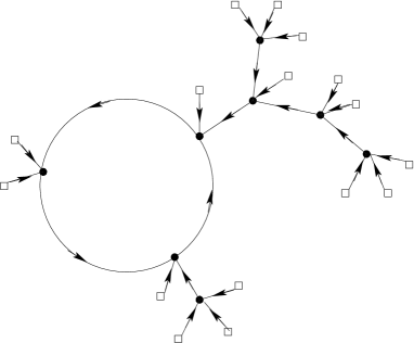
Figure 1: A connected graph of the Gallavotti theory. Black dots are vertices and bear $\lambda$ factors, white squares bear $J$ factors and arrows point from $\bar{\phi}$ to $\phi$. Remark that three arrows point to each vertex so this is a connected graph of the $\lambda\bar{\phi}\phi^{3}+\bar{\phi}J$ theory.

We can therefore identify the free energy ${\cal A}_{p}(\lambda,J)=\log Z^{G}_{p}(\lambda,J)$ of that theory to the same sum restricted to connected graphs, hence to a sum over single oriented cycles of arbitrary length $q$ (with regular associated cycle weight $\frac{1}{q}$) decorated with oriented regular p-ary trees pointing towards the cycles. We therefore understand that the computations of section II correspond to force integration over a single $\bar{\phi}$ field per vertex, keeping all others as frozen spectators.

A graphical representation of the action of the previous section can be deduced by changing the sign of $\lambda$, substituting factors $\phi$ for each $J$ factor and adding a factor $\bar{\phi}^{p-1}$ at each node, see Figure 2. In other words

$$S_{p}(g,\phi,\bar{\phi})={\cal A}_{p}(\lambda,J)|_{J=\phi,\lambda=g^{p}\bar{\phi}^{p-1}}.$$ (IV-31)

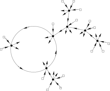
Figure 2: The same connected graph but reinterpreted for the $(\bar{\phi}\phi)^{3}$ theory. White squares are now $\phi$ factors, outgoing arrows are factors $\bar{\phi}$. Remark that each vertex is now 6-valent.

We think these figures show also convincingly how the method extends to other $(\bar{\phi}\phi)^{p}$-type theories with more complicated multidimensional Gaussian measures having less trivial propagators $\Gamma$, such as those required by usual $d$-dimensional field theories with inverse Laplacian propagator or by matrix and tensor models and field theories. Simply add these propagators on the edges of the graphs in Figures 1-2. Such extensions will be studied in future publications. Of course we can also perform such computations for Fermionic theories with Berezin variables, but the constructive theory in that case is simpler since sign cancellations make the perturbative expansion directly summable.

Remark that in the scalar case arrows can be hooked in any way at the vertices but in the case of $N$ by $N$ matrix models [1] and [11] or tensor models of rank $r$ with $N^{r}$ coefficients, edges should be stranded and cyclic alternation of arrows at each vertex or insertions on strands of the correct color [6, 12] should be respected. This will be crucial to ensure analytic estimates with the correct scaling in $N$.

V Loop Vertex Expansion

We can then set up the exact analog of the loop vertex expansion for this model. For simplicity let us compute only $\log Z$. Starting from (II-19) and applying the LVE gives, in the notations of [42]:

$$Z_{p}(\lambda) = \sum_{n}\int d\mu(\phi,\bar{\phi})\frac{S_{p}^{n}}{n!}$$ (V-32)

$$= \sum_{n}\frac{1}{n!}\sum_{{\cal{F}}}\int dw_{\cal{F}}\int d\mu_{{\cal{F}},w}(\phi,\bar{\phi})\partial_{\cal{F}}\prod_{i=1}^{n}S_{p}(\lambda,\phi_{i},\bar{\phi}_{i})$$ (V-33)

where

• the sum over ${\cal{F}}$ is over oriented forests over $n$ labeled vertices $v=1,\cdots,n$, including the empty forest with no edge. Such forests are exactly the acyclic oriented edge-subgraphs of the complete graph $K_{n}$.

• $\int dw_{\cal{F}}$ means integration from 0 to 1 over one parameter for each forest edge: $\int dw_{\cal{F}}\equiv\prod_{\ell\in{\cal{F}}}\int_{0}^{1}dw_{\ell}$. There is no integration for the empty forest since by convention an empty product is 1. A generic integration point $w_{\cal{F}}$ is therefore made of $|{\cal{F}}|$ parameters $w_{\ell}\in[0,1]$, one for each $\ell\in{\cal{F}}$.

• $\partial_{\cal{F}}=\prod_{\ell\in{\cal{F}}}\frac{\partial}{\partial\bar{\phi}_{i(\ell)}}\frac{\partial}{\partial\phi_{j(\ell)}}$ means a product of first order partial derivatives with respect to the variables $\bar{\phi}_{i(\ell)}$ and $\phi_{j(\ell)}$ corresponding to the departure vertex $i(\ell)$ and arrival vertex $j(\ell)$ of the oriented line $\ell\in{\cal{F}}$. Again there is no such derivatives for the empty forest since by convention an empty product is 1.

• $d\mu_{{\cal{F}},w}(\phi,\bar{\phi})$ is the Gaussian measure on the replica variables $(\phi_{i},\bar{\phi}_{i})$ for $i\in\{1,\cdots,n\}$ with covariance $X^{\cal{F}}(w_{\cal{F}})$, which for $i\neq j$, is the infimum of the $w_{\ell}$ parameters for $\ell$ in the unique path $P^{\cal{F}}_{i\to j}$ from $i$ to $j$ in ${\cal{F}}$. If no such path exists, hence $i$ and $j$ belong to different connected components of the forest ${\cal{F}}$, then by convention $X^{\cal{F}}_{ij}(w_{\cal{F}})=0$. Finally for all $i$ $X^{\cal{F}}_{ii}(w_{\cal{F}}):=1$.

Remember that the symmetric $n$ by $n$ matrix $X^{\cal{F}}(w_{\cal{F}})$ defined in this way is positive for any value of $w_{\cal{F}}$ so that this formula is well-defined.

Then the formula factorizes over the trees which are the connected components of ${\cal{F}}$ so that

$$\log Z_{p}(\lambda) = \sum_{n}\frac{1}{n!}\sum_{{\cal{T}}}\int dw_{\cal{T}}\int d\mu_{{\cal{T}},w}(\phi,\bar{\phi})\partial_{\cal{T}}\prod_{i=1}^{n}S_{p}(z_{i})$$ (V-34)

where the sum over ${\cal{T}}$ runs now only over spanning trees over the $n$ labeled vertices $i=1,\cdots,n$, and $z_{i}=-\lambda(\phi_{i}\bar{\phi}_{i})^{p-1}$ where $(\phi_{i},\bar{\phi}_{i})$ are the replica variables at vertex $i$.

Theorem V.1.

For any $\epsilon>0$ there exists $\eta$ small enough such that the sum (V-34) is absolutely convergent in the “pacman domain”

$$P(\epsilon,\eta):=\{\lambda\in D(0,\eta),|\arg\lambda|<\pi-\epsilon\}.$$ (V-35)

Proof  Using Theorem III.1, this reduces to a simple exercise in combinatorics. Indeed in bounding the series we have just to take into account that the 2$|{\cal{T}}|$ derivatives associated to the tree corners will create local factorials $(d_{i}-1)!$ in the degree of the tree at vertex $i$. At each vertex of coordination $d_{i}$ in the tree the $d_{i}$ derivatives with respect to the $\phi_{i}$ or $\bar{\phi}_{i}$ variables in $\partial_{\cal{T}}$ create indeed a sum of at most $K^{d_{i}}(d_{i}-1)!$ monomials of the type $(-\lambda)^{r_{i}}\phi^{s_{i}}\bar{\phi}^{t_{i}}S^{(r_{i})}(z_{i})$ with $\sup\{1,\frac{d_{i}}{2p-2}\}\leq r_{i}\leq d_{i}$ and $s_{i}+t_{i}=(2p-3)r_{i}-(d_{i}-r_{i})=(2p-2)r_{i}-d_{i}$ But using (III-20) this sum is therefore bounded by

$$(d_{i}-1)!K^{d_{i}}\bigl{[}\frac{K_{p}(\epsilon)}{1+|z_{i}|}\bigr{]}^{r_{i}}|z_{i}|^{r_{i}-\frac{d_{i}}{2p-2}}|\lambda|^{\frac{d_{i}}{2p-2}}\leq(d_{i}-1)![KK_{p}(\epsilon)]^{d_{i}}|\lambda|^{\frac{d_{i}}{2p-2}}.$$ (V-36)

Using Cayley’s formula for the number of trees with fixed degrees, and taking $\eta$ (hence $|\lambda|$) in Theorem V.1 small enough achieves the proof. Notice however that as usual, the case ${\cal{T}}={\cal{T}}_{0}$, the “empty” tree reduced to a single loop vertex, requires a special treatment. Indeed $S$ itself, in contrast with its derivatives, is unbounded at large $z$, but $S(0)=0$. Hence we need to write first $S=\int_{0}^{1}zS^{\prime}(tz)dt$ and integrate by parts

$$\int d\mu_{{\cal{T}}_{0},w}(\phi,\bar{\phi})S(z)=-\lambda\int_{0}^{1}dt\int d\mu_{{\cal{T}}_{0},w}(\phi,\bar{\phi})\frac{\partial^{p-1}}{\partial\phi^{p-1}}\bigl{[}\phi^{p-1}S^{\prime}(tz)\bigr{]}$$ (V-37)

before applying the previous bounds. ∎

The convergence of the LVE for the cumulants of the theory essentially amounts to add a finite number of extra $\frac{\partial}{\partial g}$ derivatives as cilia [12] decorating the previous computation. It is left to the reader to check that these cilia do not spoil the convergence of the expansion.

Acknowledgments We thank G. Duchamp, R. Gurau, L. Lionni and A. Sokal for useful discussions.

VI Appendix: Explicit Formulas for $p$ small

VI.1 The $(\bar{\phi}\phi)^{2}$ theory

In this case $g=(-\lambda)^{\frac{1}{2}}=i\sqrt{\lambda}$, $\lambda=-g^{2}$ and $z=g^{2}\bar{\phi}\phi=-\lambda\bar{\phi}\phi$. Equation (II-14) takes the form

$$zT_{2}^{2}(z)-T_{2}(z)+1=0$$ (VI-38)

with solution the ordinary Catalan function

$$T_{2}(z)=\frac{1-\sqrt{1-4z}}{2z}.$$ (VI-39)

We find

$$F_{2}(z)=zT_{2}^{\prime}+T_{2}=(1-4z)^{-1/2}=(1-4g^{2}\bar{\phi}\phi)^{-1/2}=(1+4\lambda\bar{\phi}\phi)^{-1/2},$$ (VI-40)

and the LVR action is

$$S_{2}=-\frac{1}{2}\log(1-4z)=-\frac{1}{2}\log(1-4g^{2}\bar{\phi}\phi)=-\frac{1}{2}\log(1+4\lambda\bar{\phi}\phi).$$ (VI-41)

Its first order derivative is

$$\frac{\partial S_{2}}{\partial g}=\frac{4g\bar{\phi}\phi}{1-4g^{2}\bar{\phi}\phi}$$ (VI-42)

so that the loop vertex representation of the partition function is

$$Z_{2}(\lambda) = \int d\mu(\phi,\bar{\phi})e^{-\frac{1}{2}\log(1-4\lambda\bar{\phi}\phi)},$$ (VI-43)

$$G^{c}_{2,1}(\lambda) = 1-\frac{\lambda}{Z_{2}(\lambda)}\int d\mu(\phi,\bar{\phi})\frac{4\bar{\phi}\phi}{1+4\lambda\bar{\phi}\phi}e^{-\frac{1}{2}\log(1-4\lambda\bar{\phi}\phi)}$$ (VI-44)

$$= 1-4\lambda+\cdots.$$ (VI-45)

We recover the familiar logarithmic form of the action and resolvent of the intermediate field theory. However our LVR representation is not the intermediate field representation. Indeed in the LVR representation the argument of the log is quadratic in complex fields similar to the initial fields although it would be linear in the single real field $\sigma$ of the intermediate field representation. We should rather think to the fields of the LVR as to what remains of the initial fields after having forced integration of one particular marked $\bar{\phi}$ field per vertex.

VI.2 The $(\bar{\phi}\phi)^{3}$ theory

In this case $g=(-\lambda)^{\frac{1}{3}}=e^{i\pi/3}\lambda^{1/3}$, $\lambda=-g^{3}$ and $z=g^{3}(\bar{\phi}\phi)^{2}=-\lambda(\bar{\phi}\phi)^{2}$. Equation (II-14) is now

$$zT_{3}^{3}(x)-T_{3}(z)+1=0.$$ (VI-46)

which is soluble by radicals. Introducing

$$u:=-\frac{27z}{4}=-\frac{27}{4}g^{3}(\bar{\phi}\phi)^{2}=\frac{27}{4}\lambda(\bar{\phi}\phi)^{2},$$ (VI-47)

Cardano’s solution is

$$T_{3}(z)=\frac{\Delta_{+}(u)-\Delta_{-}(u)}{\sqrt{-3z}}=1+z+3z^{2}+\cdots,$$ (VI-48)

where

$$\Delta_{\pm}(u):=\biggl{(}\sqrt{1+u}\pm\sqrt{u}\biggr{)}^{1/3}=1\pm\frac{1}{3}\sqrt{u}+\frac{u}{18}\mp\frac{4u^{3/2}}{81}-\frac{35u^{2}}{1944}+\cdots.$$ (VI-49)

Defining $h(u):=\frac{1}{\sqrt{1+u}}$, we can compute the derivatives

$$\Delta^{\prime}_{\pm}=\frac{d}{du}\Delta_{\pm}(u) = \frac{1}{6}\biggl{(}(1+u)^{-1/2}\pm u^{-1/2}\biggr{)}\biggl{(}\sqrt{1+u}\pm\sqrt{u}\biggr{)}^{-2/3}$$ (VI-50)

$$= \pm\frac{1}{6\sqrt{u(1+u)}}\Delta_{\pm}(u)=\pm\frac{h}{6\sqrt{u}}\Delta_{\pm}(u).$$

Hence

$$zT_{3}^{\prime}(z)=\frac{27\sqrt{-z}}{4\sqrt{3}}[\Delta^{\prime}_{+}(u)-\Delta^{\prime}_{-}(u)]-\frac{1}{2\sqrt{-3z}}[\Delta_{+}(u)-\Delta_{-}(u)].$$ (VI-51)

(II-16) gives

$$F_{3} = \sum_{n}{{3n}\choose{n}}z^{n}=2zT_{3}^{\prime}+T_{3}=h\frac{\Delta_{+}+\Delta_{-}}{2},$$ (VI-52)

$$S_{3} = \log F_{3}=-\frac{1}{2}\log(1+u)+\log\frac{\Delta_{+}+\Delta_{-}}{2}$$ (VI-53)

The $u$ derivatives of $S_{3}$ give access to its $g$ derivatives since $u=-\frac{27}{4}g^{3}(\bar{\phi}\phi)^{2}$, hence

$$\frac{\partial u}{\partial g}=-\frac{81}{4}g^{2}(\bar{\phi}\phi)^{2}.$$ (VI-54)

For instance

$$\frac{\partial S_{3}}{\partial g} = \frac{81g^{2}(\bar{\phi}\phi)^{2}}{4}\biggl{(}\frac{1}{2(1+u)}-\frac{\Delta^{\prime}_{+}+\Delta^{\prime}_{-}}{\Delta_{+}+\Delta_{-}}\biggr{)}$$ (VI-55)

$$= \frac{81g^{2}(\bar{\phi}\phi)^{2}}{8}\biggl{(}h^{2}-\frac{h}{3\sqrt{u}}\frac{\Delta_{+}-\Delta_{-}}{\Delta_{+}+\Delta_{-}}\biggr{)}.$$

We remark that the quotient $\frac{\Delta_{+}-\Delta_{-}}{\Delta_{+}+\Delta_{-}}=\frac{A-B}{A+B}$ for $A=\Delta_{+}$, $B=\Delta_{-}$ simplifies, using that $(A+B)(A^{2}-AB+B^{2})=A^{3}+B^{3}$ and $(A-B)(A^{2}-AB+B^{2})=A^{3}-B^{3}-2AB(A-B)$. Remarking that in our case $AB=\Delta_{+}\Delta_{-}=1$ we find

$$\frac{\Delta_{+}-\Delta_{-}}{\Delta_{+}+\Delta_{-}} = h[\sqrt{u}-(\Delta_{+}-\Delta_{-})]$$ (VI-56)

$$\frac{\partial S_{3}}{\partial g} = \frac{81g^{2}(\bar{\phi}\phi)^{2}}{8}\biggl{(}h^{2}-\frac{h^{2}}{3\sqrt{u}}[\sqrt{u}-(\Delta_{+}-\Delta_{-})]\biggr{)}$$ (VI-57)

$$= \frac{81g^{2}(\bar{\phi}\phi)^{2}}{8}\biggl{[}\frac{2}{3}h^{2}+\frac{h^{2}}{3\sqrt{u}}(\Delta_{+}-\Delta_{-})\biggr{]}$$

$$= \frac{27g^{2}(\bar{\phi}\phi)^{2}}{4(1+u)}\biggl{[}1+\frac{\Delta_{+}-\Delta_{-}}{2\sqrt{u}}\biggr{]}$$

from which we find

$$G^{c}_{3,1}(\lambda) = 1+\frac{g}{Z_{3}(\lambda)}\int d\mu(\phi,\bar{\phi})\frac{\partial S_{3}}{\partial g}e^{S_{3}}$$ (VI-58)

$$= 1-\frac{27\lambda}{4Z_{3}(\lambda)}\int d\mu(\phi,\bar{\phi})\frac{(\bar{\phi}\phi)^{2}}{1+u}\biggl{[}1+\frac{\Delta_{+}-\Delta_{-}}{2\sqrt{u}}\biggr{]}e^{S_{3}}$$

$$= 1-18\lambda+\cdots.$$

VI.3 The $(\bar{\phi}\phi)^{4}$ theory

In this case $g=(-\lambda)^{\frac{1}{4}}=e^{i\pi/4}\lambda^{1/4}$, $\lambda=-g^{4}$ and $z=g^{4}(\bar{\phi}\phi)^{3}=-\lambda(\bar{\phi}\phi)^{3}$. Equation (II-14) is now

$$zT_{4}^{4}(z)-T_{4}(z)+1=0.$$ (VI-59)

which is still soluble by radicals. Denoting

$$v=\frac{z^{1/3}}{2^{1/3}}\Big{[}\Big{(}1+\sqrt{1-\frac{2^{8}}{3^{3}}z}\Big{)}^{1/3}+\Big{(}1-\sqrt{1-\frac{2^{8}}{3^{3}}z}\Big{)}^{1/3}\Big{]},$$ (VI-60)

then

$$T_{4}(z)=\frac{(1+4v)^{1/4}-\bigl{[}2-(1+4v)^{1/2}\bigr{]}^{1/2}}{2(vz)^{1/4}}\;.$$ (VI-61)

We can then compute

$$F_{4} = \frac{T_{4}}{4-3T_{4}}=3zT_{4}^{\prime}+T_{4}$$ (VI-62)

$$= \frac{(1+4v)^{1/4}-\bigl{[}2-(1+4v)^{1/2}\bigr{]}^{1/2}}{8(vz)^{1/4}-3\bigl{[}(1+4v)^{1/4}-\bigl{[}2-(1+4v)^{1/2}\bigr{]}^{1/2}\bigr{]}}$$

from which $S_{4}=\log F_{4}$ can be derived explicitly.

References

• [1] V. Rivasseau, “Constructive Matrix Theory,” JHEP 0709 (2007) 008 [arXiv:0706.1224 [hep-th]].
• [2] D. Brydges and T. Kennedy, Mayer expansions and the Hamilton-Jacobi equation, Journal of Statistical Physics, 48, 19 (1987).
• [3] A. Abdesselam and V. Rivasseau, “Trees, forests and jungles: A botanical garden for cluster expansions,” arXiv:hep-th/9409094.
• [4] V. Rivasseau and Z. Wang, “How to Resum Feynman Graphs,” Annales Henri Poincare 15, no. 11, 2069 (2014) doi:10.1007/s00023-013-0299-8 [arXiv:1304.5913 [math-ph]].
• [5] R. Gurau and J. P. Ryan, SIGMA 8, 020 (2012) doi:10.3842/SIGMA.2012.020 [arXiv:1109.4812 [hep-th]].
• [6] R. Gurau, “Random Tensors”, Oxford University Press (2016).
• [7] G. ’t Hooft, “A PLANAR DIAGRAM THEORY FOR STRONG INTERACTIONS,” Nucl. Phys. B 72, 461 (1974).
• [8] R. Gurau, “The 1/N expansion of colored tensor models,” Annales Henri Poincare 12, 829 (2011) doi:10.1007/s00023-011-0101-8 [arXiv:1011.2726 [gr-qc]].
• [9] R. Gurau and V. Rivasseau, “The 1/N expansion of colored tensor models in arbitrary dimension,” Europhys. Lett.  95, 50004 (2011) doi:10.1209/0295-5075/95/50004 [arXiv:1101.4182 [gr-qc]].
• [10] R. Gurau, “The complete 1/N expansion of colored tensor models in arbitrary dimension,” Annales Henri Poincare 13, 399 (2012) doi:10.1007/s00023-011-0118-z [arXiv:1102.5759 [gr-qc]].
• [11] R. Gurau and T. Krajewski, “Analyticity results for the cumulants in a random matrix model,” arXiv:1409.1705 [math-ph].
• [12] R. Gurau, “The 1/N Expansion of Tensor Models Beyond Perturbation Theory,” Commun. Math. Phys.  330, 973 (2014) doi:10.1007/s00220-014-1907-2 [arXiv:1304.2666 [math-ph]].
• [13] T. Delepouve, R. Gurau and V. Rivasseau, “Universality and Borel Summability of Arbitrary Quartic Tensor Models,” arXiv:1403.0170 [hep-th].
• [14] R. Gurau and V. Rivasseau, “The Multiscale Loop Vertex Expansion,” Annales Henri Poincaré 16, no. 8, 1869 (2015) [arXiv:1312.7226 [math-ph]].
• [15] T. Delepouve and V. Rivasseau, “Constructive Tensor Field Theory: The $T^{4}_{3}$ Model,” arXiv:1412.5091 [math-ph].
• [16] V. Lahoche, “Constructive Tensorial Group Field Theory II: The $U(1)-T^{4}_{4}$ Model,” arXiv:1510.05051 [hep-th].
• [17] J. Magnen and V. Rivasseau, “Constructive $\phi^{4}$ field theory without tears,” Annales Henri Poincare 9 (2008) 403 [arXiv:0706.2457 [math-ph]].
• [18] V. Rivasseau and Z. Wang, “Corrected loop vertex expansion for $\Phi_{2}^{4}$ theory,” J. Math. Phys.  56, no. 6, 062301 (2015) doi:10.1063/1.4922116 [arXiv:1406.7428 [math-ph]].
• [19] V. Rivasseau and Z. Wang, “Loop Vertex Expansion for Phi**2K Theory in Zero Dimension,” J. Math. Phys.  51, 092304 (2010) doi:10.1063/1.3460320 [arXiv:1003.1037 [math-ph]].
• [20] L. Lionni and V. Rivasseau, “Note on the Intermediate Field Representation of $\phi^{2k}$ Theory in Zero Dimension”, arXiv:1601.02805.
• [21] L. Lionni and V. Rivasseau, “Intermediate Field Representation for Positive Matrix and Tensor Interactions,” arXiv:1609.05018 [math-ph].
• [22] G. Gallavotti, “Perturbation Theory”, In: Mathematical physics towards the XXI century, 275-294, R. Sen and A. Gersten, eds., Ber Sheva, Ben Gurion University Press, 1994.
• [23] W. Mlotkowski and K. A. Penson, “Probability distributions with binomial moments”, in Infinite Dimensional Analysis, Quantum Probability and Related Topics, Vol. 17, No. 2 (2014) 1450014, World Scientific.
• [24] V. Bonzom, R. Gurau, A. Riello and V. Rivasseau, “Critical behavior of colored tensor models in the large N limit,” Nucl. Phys. B 853, 174 (2011) doi:10.1016/j.nuclphysb.2011.07.022 [arXiv:1105.3122 [hep-th]].
• [25] V. Rivasseau, “Quantum Gravity and Renormalization: The Tensor Track,” arXiv:1112.5104.
• [26] V. Rivasseau, “The Tensor Track: an Update,” arXiv:1209.5284.
• [27] V. Rivasseau, “The Tensor Track, III,” Fortsch. Phys.  62, 81 (2014) doi:10.1002/prop.201300032 [arXiv:1311.1461 [hep-th]].
• [28] V. Rivasseau, “The Tensor Track, IV,” PoS CORFU 2015, 106 (2016) [arXiv:1604.07860 [hep-th]].
• [29] V. Rivasseau, “Random Tensors and Quantum Gravity,” SIGMA 12, 069 (2016) doi:10.3842/SIGMA.2016.069 [arXiv:1603.07278 [math-ph]].
• [30] E. Witten, “An SYK-Like Model Without Disorder,” arXiv:1610.09758 [hep-th].
• [31] R. Gurau, “The complete $1/N$ expansion of a SYK-like tensor model,” Nucl. Phys. B 916, 386 (2017) doi:10.1016/j.nuclphysb.2017.01.015 [arXiv:1611.04032 [hep-th]].
• [32] I. R. Klebanov and G. Tarnopolsky, “Uncolored Random Tensors, Melon Diagrams, and the SYK Models,” arXiv:1611.08915 [hep-th].
• [33] C. Krishnan, S. Sanyal and P. N. Bala Subramanian, “Quantum Chaos and Holographic Tensor Models,” arXiv:1612.06330 [hep-th].
• [34] F. Ferrari, “The Large D Limit of Planar Diagrams,” arXiv:1701.01171 [hep-th].
• [35] R. Gurau, “Quenched equals annealed at leading order in the colored SYK model,” arXiv:1702.04228 [hep-th].
• [36] V. Bonzom, L. Lionni and A. Tanasa, “Diagrammatics of a colored SYK model and of an SYK-like tensor model, leading and next-to-leading orders,” arXiv:1702.06944 [hep-th].
• [37] J. Ben Geloun and V. Rivasseau, “A Renormalizable 4-Dimensional Tensor Field Theory,” Commun. Math. Phys.  318, 69 (2013) doi:10.1007/s00220-012-1549-1 [arXiv:1111.4997 [hep-th]].
• [38] S. Carrozza, D. Oriti and V. Rivasseau, “Renormalization of a SU(2) Tensorial Group Field Theory in Three Dimensions,” Commun. Math. Phys.  330, 581 (2014) doi:10.1007/s00220-014-1928-x [arXiv:1303.6772 [hep-th]].
• [39] D. Perrin, private communication.
• [40] H. Osada, “The Galois group of the Polynomials $X^{n}+aX^{\prime}+b$”, Journal of number theory 25 230-238 (1987).
• [41] A. D. Sokal, “An Improvement Of Watson’s Theorem On Borel Summability,” J. Math. Phys.  21, 261 (1980).
• [42] V. Rivasseau, “Constructive Tensor Field Theory,” SIGMA 12, 085 (2016) doi:10.3842/SIGMA.2016.085 [arXiv:1603.07312 [math-ph]].