Current Challenges in Developing Open Source Computer Algebra Systems

Abstract.

This note is based on the plenary talk given by the second author at MACIS 2015, the Sixth International Conference on Mathematical Aspects of Computer and Information Sciences. Motivated by some of the work done within the Priority Programme SPP 1489 of the German Research Council DFG, we discuss a number of current challenges in the development of Open Source computer algebra systems. The main focus is on algebraic geometry and the system Singular.

1. Introduction

The goal of the nationwide Priority Programme SPP 1489 of the German Research Council DFG is to considerably further the algorithmic and experimental methods in algebraic geometry, number theory, and group theory, to combine the different methods where needed, and to apply them to central questions in theory and practice. In particular, the programme is meant to support the further development of Open Source computer algebra systems which are (co-)based in Germany, and which in the framework of different projects may require crosslinking on different levels. The cornerstones of the latter are the well-established systems GAP [34] (group and representation theory), polymake [35] (polyhedral geometry), and Singular [25] (algebraic geometry, singularity theory, commutative and non-commutative algebra), together with the newly evolving system ANTIC [41] (number theory), but there are many more systems, libraries, and packages involved (see Section 2.4 for some examples).

In this note, having the main focus on Singular, we report on some of the challenges which we see in this context. These range from reconsidering the efficiency of the basic algorithms through parallelization and making abstract concepts constructive to facilitating the access to Open Source computer algebra systems. In illustrating the challenges, which are discussed in Section 2, we take examples from algebraic geometry. In Sections 3 and Section 4, two of the examples are highlighted in more detail. These are the parallelization of the classical Grauert-Remmert type algorithms for normalization and the computation of GIT-fans. The latter is a show-case application of bringing Singular, polymake, and GAP together.

2. Seven Challenges

2.1. Reconsidering the Efficiency of the Basic Algorithms

Motivated by an increasing number of success stories in applying algorithmic and experimental methods to algebraic geometry (and other areas of mathematics), research projects in this direction become more and more ambitious. This applies both to the theoretical level of abstraction and to the practical complexity. On the computer algebra side, this not only requires innovative ideas to design high-level algorithms, but also to revise the basic algorithms on which the high-level algorithms are built. The latter concerns efficiency and applicability.

Example 1 (The Nemo project).

Nemo is a new computer algebra package written in the Julia programming language which, in particular, aims at highly efficient implementations of basic arithmetic and algorithms for number theory and is connected to the ANTIC project. See http://nemocas.org/index.html for some benchmarks.

In computational algebraic geometry, aside from polynomial factorization, the basic work horse is Buchberger’s algorithm for computing Gröbner bases [22] and, as remarked by Schreyer [46] and others, syzygies. While Gröbner bases are specific sets of generators for ideals and modules which are well-suited for computational purposes, the name syzygies refers to the relations on a given set of generators. Syzygies carry important geometric information (see [28]) and are crucial ingredients in many basic and high-level algorithms. Taking syzygies on the syzygies and so forth, we arrive at what is called a free resolution. Here is a particular simple example.

Example 2 (The Koszul complex of Three Variables).

In the Singular session below, we first construct the polynomial ring $R=\mathbb{Q}[x,y,z]$, endowed with the degree reverse lexicographical order dp. Then we compute the successive syzygies on the variables $x,y,z$.

$\color[rgb]{0,0,1}>$ ring R = 0, (x,y,z), dp;

$\color[rgb]{0,0,1}>$ ideal I = x,y,z;

$\color[rgb]{0,0,1}>$ resolution FI = nres(I,0);

$\color[rgb]{0,0,1}>$ print(FI[2]);

0,-y,-z,

-z, x, 0,

y, 0, x

$\color[rgb]{0,0,1}>$ print(FI[3]);

x,

z,

-y

In the following example, we show how Gröbner basis and syzygy computations fit together to build a more advanced algorithm.

Example 3 (Parametrizing Rational Curves).

We study a degree-5 curve $C$ in the projective plane which is visualized as the red curve in Figures 1 and 2. To begin with, after constructing the polynomial ring $R=\mathbb{Q}[x,y,z]$, we enter the homogeneous degree-5 polynomial $f\in\mathbb{Q}[x,y,z]$ which defines $C$:

$\color[rgb]{0,0,1}>$ ring R = 0, (x,y,z), dp;

$\color[rgb]{0,0,1}>$ poly f = x5+10x4y+20x3y2+130x2y3-20xy4+20y5-2x4z-40x3yz

                 -150x2y2z-90xy3z-40y4z+x3z2+30x2yz2+110xy2z2+20y3z2;

Our goal is to check whether $C$ is rational, and if so, to compute a rational parametrization. For the first task, recall that an algebraic curve is rational if and only if its geometric genus is zero. In the example here, this can be easily read off from the genus formula for plane curves, taking into account that the degree-5 curve has three ordinary double points and one ordinary triple point (see the aforementioned visualization). An algorithm for computing the genus in general, together with an algorithm for computing rational parametrizations, is implemented in the Singular library paraplanecurves.lib [15]:

$\color[rgb]{0,0,1}>$ LIB "paraplanecurves.lib";

$\color[rgb]{0,0,1}>$ genus(f);

0

$\color[rgb]{0,0,1}>$ paraPlaneCurve(f);

Rather than displaying the result, we will now show the key steps of the algorithm at work. The first step is to compute the ideal generated by the adjoint curves of $C$ which, roughly speaking, are curves which pass with sufficiently high multiplicity through the singular points of $C$. The algorithm for computing the adjoint ideal (see [11]) builds on algorithms for computing normalization (see Section 3) or, equivalently, integral bases (see [10]). In all these algorithms, Gröbner bases are used as a fundamental tool.

$\color[rgb]{0,0,1}>$ ideal AI = adjointIdeal(f);

$\color[rgb]{0,0,1}>$ AI;

_[1]=y3-y2z

_[2]=xy2-xyz

_[3]=x2y-xyz

_[4]=x3-x2z

The resulting four cubic generators of the adjoint ideal define the curves depicted in Figure 1, where the thickening of a line indicates that the line comes with a double structure. A general adjoint curve, that is, a curve defined by a general linear combination of the four generators, is shown in Figure 2.

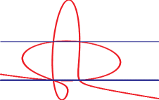
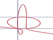
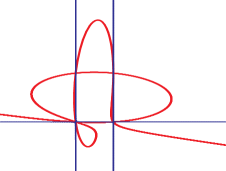
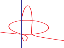
Figure 1. Cubic curves defined by the generators of the adjoint ideal of a degree-$5$ curve with three ordinary double points and one ordinary triple point. The degree-5 curve is shown in red.

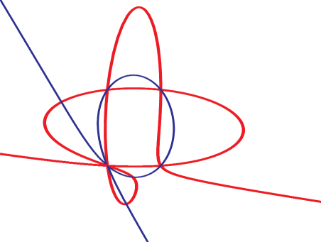
Figure 2. A general adjoint curve of $C$ of degree $3$.

The four generators give a birational map from $C$ to a curve $\widetilde{C}$ in projective 3-space $\mathbb{P}^{3}$. We obtain $\widetilde{C}$ via elimination, a typical application of Gröbner bases:

$\color[rgb]{0,0,1}>$ def Rn = mapToRatNormCurve(f,AI);

$\color[rgb]{0,0,1}>$ setring(Rn);

$\color[rgb]{0,0,1}>$ RNC;

RNC[1]=y(2)*y(3)-y(1)*y(4)

RNC[2]=20*y(1)*y(2)-20*y(2)^2+130*y(1)*y(4)

+20*y(2)*y(4)+10*y(3)*y(4)+y(4)^2

RNC[3]=20*y(1)^2-20*y(1)*y(2)+130*y(1)*y(3)

+10*y(3)^2+20*y(1)*y(4)+y(3)*y(4)

Note that $\widetilde{C}$ is a variant of the projective twisted cubic curve, the rational normal curve in $\mathbb{P}^{3}$ (for a picture see Figure 10). This non-singular curve is mapped isomorphically onto the projective line $\mathbb{P}^{1}$ by the anticanonical linear system, which can be computed using syzygies:

$\color[rgb]{0,0,1}>$ rncAntiCanonicalMap(RNC);

_[1]=2*y(2)+13*y(4)

_[2]=y(4)

Composing all maps in this construction, and inverting the resulting birational map, we get the desired parametrization. In general, depending on the number of generators of the adjoint ideal, the rational normal curve computed by the algorithm is embedded into a projective space of odd or even dimension. In the latter case, successive applications of the canonical linear system map the normal curve onto a plane conic. Computing a rational parametrization of the conic is equivalent to finding a point on the conic. It can be algorithmically decided whether we can find such a point with rational coordinates or not. In the latter case, we have to pass to a quadratic field extension of $\mathbb{Q}$.

Remark 4.

The need of passing to a field extension occurs in many geometric constructions. Often, repeated field extensions are needed. The effective computation of Gröbner bases over (towers of) number fields is therefore of utmost importance. One general way of achieving higher speed is the parallelization of algorithms. This will be addressed in the next section, where we will, in particular, discuss a parallel version of the Gröbner basis (syzygy) algorithm which is specific to number fields [18]. New ideas for enhancing syzygy computations in general are presented in [31]. Combining the two approaches in the case of number fields is a topic of future research.

2.2. Parallelization

Parallelizing computer algebra systems allows for the efficient use of multicore computers and high-performance clusters. To achieve parallelization is a tremendous challenge both from a computer science and a mathematical point of view.

From a computer science point of view, there are two possible approaches:

• Distributed and multi-process systems work by using different processes that do not share memory and communicate by message passing. These systems only allow for coarse-grained parallelism, which limits their ability to work on large shared data structures, but can in principle scale up indefinitely.

• Shared memory systems work by using multiple threads of control in a single process operating on shared data. They allow for more fine-grained parallelism and more sophisticated concurrency control, down to the level of individual CPU instructions, but are limited in their scalability by how many processors can share efficient access to the same memory on current hardware.

For best performance, typically hybrid models are used, which exploit the strengths of both shared memory and distributed systems, while mitigating their respective downsides.

From its version 3.1.4 on, Singular has been offering a framework for coarse-grained parallelization, with a convenient user access provided by the library parallel.lib [48]. The example below illustrates the use of this framework:

Example 5 (Coarse Grained Parallelization in Singular).

We implement a Singular procedure which computes a Gröbner basis for a given ideal with respect to a given monomial ordering. The procedure returns the size of the Gröbner basis. We apply it in two parallel runs to a specific ideal in $\mathbb{Q}[x_{1},\dots,x_{4}]$, choosing for one run the lexicographical monomial ordering lp and for the other run the degree reverse lexicographical ordering dp:

$\color[rgb]{0,0,1}>$ LIB "parallel.lib"; LIB "random.lib";

$\color[rgb]{0,0,1}>$ proc sizeGb(ideal I, string monord){

def R = basering; list RL = ringlist(R);

RL[3][1][1] = monord; def S = ring(RL); setring(S);

return(size(groebner(imap(R,I))));}

$\color[rgb]{0,0,1}>$ ring R = 0,x(1..4),dp;

$\color[rgb]{0,0,1}>$ ideal I = randomid(maxideal(3),3,100);

$\color[rgb]{0,0,1}>$ list commands = "sizeGb","sizeGb";

$\color[rgb]{0,0,1}>$ list args = list(I,"lp"),list(I,"dp");

$\color[rgb]{0,0,1}>$ parallelWaitFirst(commands, args);

[1] empty list

[2] 11

$\color[rgb]{0,0,1}>$ parallelWaitAll(commands, args);

[1] 55

[2] 11

As expected, the computation with respect to dp is much faster and leads to a Gröbner basis with less elements.

Using ideas from the successful parallelization of GAP within the HPC-GAP project (see [4, 5, 6]), a multi-threaded prototype of Singular has been implemented. Considerable further efforts are needed, however, to make this accessible to users without a deep background in parallel programming.

From a mathematical point of view, there are algorithms whose basic strategy is inherently parallel, whereas others are sequential in nature. A prominent example of the former type is Villamayor’s constructive version of Hironaka’s desingularization theorem, which will be briefly discussed in Section 2.3. A prominent example of the latter type is the classical Grauert-Remmert type algorithm for normalization, which will be addressed at some length in Section 3.

The systematic design of parallel algorithms for applications which so far can only be handled by sequential algorithms is a major task for the years to come. For normalization, this problem has recently been solved [14]. Over the field of rational numbers, the new algorithm becomes particularly powerful by combining it with modular methods, see again Section 3.

Modular methods are well-known for providing a way of parallelizing algorithms over $\mathbb{Q}$ (more generally, over number fields). For the fundamental task of computing Gröbner bases, a modular version of Buchberger’s algorithm is due to Arnold [1]. More recently, Boku, Fieker, Steenpaß and the second author [18] have designed a modular Gröbner bases algorithm which is specific to number fields. In addition to using the approach from Arnold’s paper, which is to compute Gröbner bases modulo several primes and then use Chinese remaindering together with rational reconstruction, the new approach provides a second level of parallelization as depicted in Figure 3: If the number field is presented as $K=\mathbb{Q}(\alpha)=\mathbb{Q}[t]/\langle f\rangle$, where $f\in\mathbb{Q}[t]$ is the minimal polynomial of $\alpha$, and if generators $g_{1}(X,\alpha),\dots,g_{s}(X,\alpha)$ for the ideal under consideration are given, represented by polynomials $g_{1}(X,t),\dots,g_{s}(X,t)\in\mathbb{Q}[X,t]=Q[x_{1},\dots,x_{n},t]$, we wish to compute a Gröbner basis for the ideal $\widetilde{I}=\langle g_{1}(X,t),\dots,g_{s}(X,t),f\rangle\subset\mathbb{Q}[X,t]$. The idea then is to reduce $\widetilde{I}$ modulo a suitable number of primes $p_{1},\dots,p_{k}$ (level 1 of the algorithm), get the second level of parallelization by factorizing the reductions of $f$ modulo the $p_{i}$, and use, for each $i$, polynomial Chinese remaindering to put the results modulo $p_{i}$ together (level 3 of the algorithm).

Figure 3. Two-fold parallel modular approach to Gröbner bases over number fields.

2.3. Make More and More of the Abstract Concepts of Algebraic Geometry Constructive

The following groundbreaking theorem proved by Hironaka in $1964$ shows the existence of resolutions of singularites in characteristic zero. It is worth mentioning that, on his way, Hironaka introduced the idea of standard bases, the power series analogue of Gröbner bases.

Theorem 6 (Hironaka, 1964).

For every algebraic variety over a field $K$ of characteristic zero, a desingularization can be obtained by a finite sequence of blow-ups along smooth centers.

We illustrate the blow-up process by a simple example:

Example 7.

As shown in Figure 4, a node can be resolved by a single blow-up: we replace the node by a line and separate, thus, the two branches of the curve intersecting in the singularity.

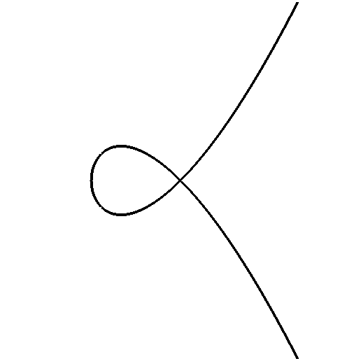
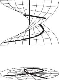
Figure 4. Blowing up a node.

In [9, 20, 30, 32], the abstract concepts developed by Hironaka have been translated into an algorithmic approach to desingularization. An effective variant of this, relying on a clever selection of the centers for the blow-ups, has been implemented by Frühbis-Krüger and Pfister in the Singular library resolve.lib [33].

The desingularization algorithm is parallel in nature: Working with blow-ups means to work with different charts of projective spaces. In this way, the resolution of singularities leads to a tree of charts. Figure 6 shows the graph for resolving the singularities of the hypersurface $z^{2}-x^{2}y^{2}=0$ which, in turn, is depicted in Figure 5.

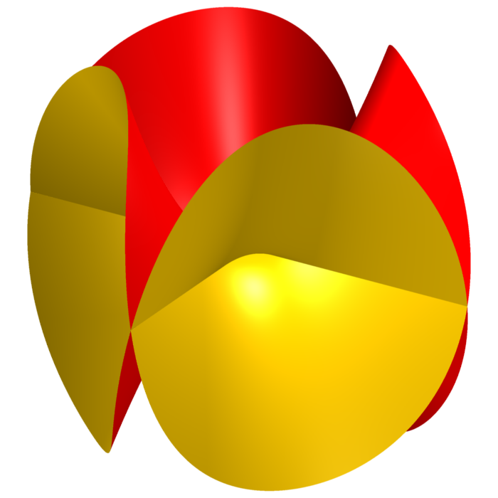
Figure 5. The surface $z^{2}-x^{2}y^{2}=0$.

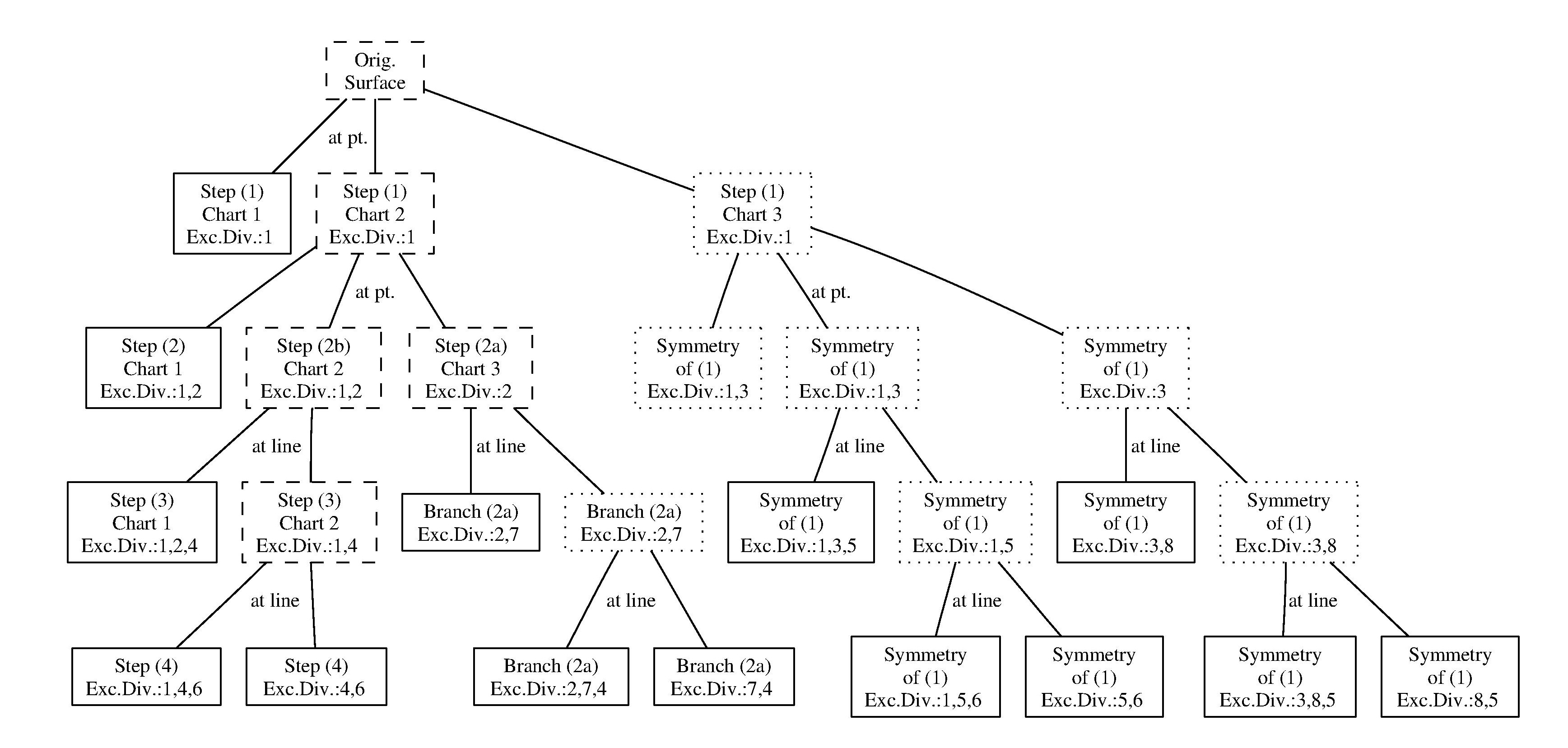
Figure 6. The tree of charts.

Making abstract concepts constructive allows for both a better understanding of deep mathematical results and a computational treatment of the concepts. A further preeminent example for this is the constructive version of the Bernstein-Gel’fand-Gel’fand correspondence (BGG-correspondence) by Eisenbud, Fløystad, and Schreyer [29]. This allows one to express properties of sheaves over projective spaces in terms of exterior algebras. More precisely, if $\mathbb{P}(V)$ is the projective space of lines in a vector space $V$, and $E$ is the exterior algebra $E=\Lambda V$, then the BGG-correspondence relates coherent sheaves over $\mathbb{P}(V)$ to free resolutions over $E$. Since $E$ contains only finitely many monomials, (non-commutative) Gröbner basis and syzygy computations over $E$ are often preferable to (commutative) Gröbner basis and syzygy computations over the homogeneous coordinate ring of $\mathbb{P}(V)$. One striking application of this, which is implemented in Macaulay2 [37] and Singular, gives a fast way of computing sheaf cohomology. Providing computational access to cohomology in all its disguises is a long-term goal of computational algebraic geometry.

The BGG-correspondence is an example of an equivalence of derived categories. As we can see from the above discussion, such equivalences are not only interesting from a theoretical point of view, but may also allow for creating more effective algorithms – provided they can be accessed computationally.

2.4. Interaction and Integration of Computer Algebra Systems and Libraries From Different Areas of Research

On the theoretical side, mathematical breakthroughs are often obtained by combining methods from different areas of mathematics. Making such connections accessible to computational methods is another major challenge. Handling this challenge requires, in particular, that computer algebra systems specializing in different areas are connected in a suitable way. One goal of the Priority Programme SPP 1489, which was already mentioned in the introduction, is to interconnect GAP, polymake, Singular, and Antic. So far, this has lead to directed interfaces as indicated in Figure 7, with further directions and a much tighter integration of the systems subject to future development.

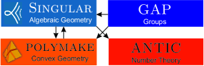
Figure 7. Directed interfaces.

In fact, the picture is much more complicated: The four systems rely on further systems and libraries such as normaliz [21] (affine monoids) and Flint [42] (number theory), and there are other packages which use at least one of the four systems, for example homalg [49] (homological algebra) and a-tint [40] (tropical intersection theory) (Figure 8).

Figure 8. The Tropicalization of Clebsch’s diagonal cubic.

With regard to mathematical applications, the value of connecting GAP and Singular is nicely demonstrated by Barakat’s work on a several years old question of Serre to find a prediction for the number of connected components of unitary groups of group algebras in characteristic 2 [47, 3].

A showcase application for combining Singular, polymake, and GAP is the symmetric algorithm for computing GIT-fans [17] by the first, third and fourth author [17]. This algorithm, which will be discussed in more detail in Section 4, combines Gröbner basis and convex hull computations, and can make use of actions of finite symmetry groups.

2.5. A Convenient Hierarchy of Languages

Most modern computer algebra systems consist of two major components, a kernel which is typically written in C/C++ and a high level language for direct user interaction, which in particular provides a convenient way for users to extend the system. While the kernel code is precompiled and, thus, performant, the user language is interpreted, which means that it operates at a significantly slower speed. In addition to the differences in speed, the languages involved provide different levels of abstraction with regard to modeling mathematical concepts. In view of the integration of different systems, a number of languages has to be considered, leading to an even more complicated situation. To achieve the required level of performance and abstraction in this context, we need to set up a convenient hierarchy of languages. Here, we propose in particular to examine the use of just-in-time compiled languages such as Julia.

2.6. Create and Integrate Electronic Libraries and Databases Relevant to Research

Electronic libraries and databases of certain classes of mathematical objects provide extremely useful tools for research in their respective fields. An example from group theory is the SmallGroups library, which is distributed as a GAP package. An example from algebraic geometry is the Graded Ring Database, written by Gavin Brown and Alexander Kasprzyk, with contributions by several other authors. The creation of such databases often depends on several computer algebra systems. On the other hand, a researcher using the data may wish to access the database within a system with which he is already familiar. This illustrates the benefits of a standardized approach to connect computer algebra systems and mathematical databases.

2.7. Facilitating the Access to Computer Algebra Systems

Computational algebraic geometry (and computer algebra in general) has a rapidly increasing amount of applications outside its original core areas, for example to computational biology, algebraic vision, and physics. As more and more non-specialists wish to use computer algebra systems, the question of how to considerably ease the access to the systems arises also in the Open Source community. Virtual research environments such as the one developed within the OpenDreamKit project may provide an answer to this question. Creating Jupyter notebooks for systems such as GAP and Singular is one of the many goals of this project. A Singular prototype has been written by Sebastian Gutsche, see Figure 9.

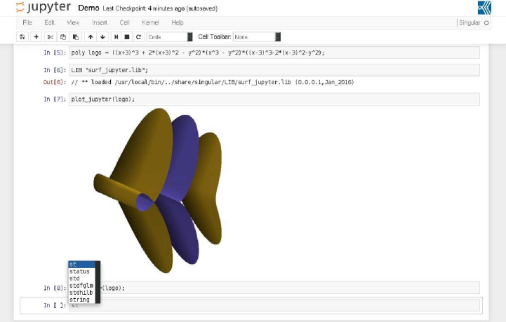
Figure 9. Jupyter notebook for Singular.

3. A Parallel Approach to Normalization

In this section, focusing on the normalization of rings, we give an example of how ideas from commutative algebra can be used to turn a sequential algorithm into a parallel algorithm.

The normalization of rings is an important concept in commutative algebra, with applications in algebraic geometry and singularity theory. Geometrically, normalization removes singularities in codimension one and “improves” singularities in higher codimension. In particular, for curves, normalization yields a desingularization (see Examples 10 and 14 below). From a computer algebra point of view, normalization is fundamental to quite a number of algorithms with applications in algebra, geometry, and number theory. In Example 3, for instance, we have used normalization to compute adjoint curves and, thus, parametrizations of rational curves.

The by now classical Grauert-Remmert type approach [23, 24, 38] to compute normalization proceeds by successively enlarging the given ring until the Grauert-Remmert normality criterion [36] tells us that the normalization has been reached. Obviously, this approach is completely sequential in nature. As already pointed out, it is a major challenge to systematically design parallel alternatives to basic and high-level algorithms which are sequential in nature. For normalization, this problem has recently been solved in [14] by using the technique of localization and proving a local version of the Grauert-Remmert normality criterion.

To explain this in more detail, we suppose for simplicity that the ring under consideration is an affine domain over a field $K$. That is, we consider a quotient ring of type $A=K[x_{1},\ldots,x_{n}]/I$, where $I$ is a prime ideal. We require that $K$ is a perfect field.

We begin by recalling some basic definitions and results.

Definition 8.

The normalization of $A$ is the integral closure $\overline{A}$ of $A$ in its quotient field $Q(A)$,

$$\overline{A}=\{a\in Q(A)\mid\text{there exists }f\in A[t]\text{ monic with }f(a)=0\}.$$

We call $A$ normal if $A=\overline{A}$.

By Emmy Noether’s finiteness theorem (see [43]), we may represent $\overline{A}$ as the set of $A$-linear combinations of a finite set of elements of $\overline{A}$. That is:

Theorem 9 (Emmy Noether).

$\overline{A}$ is a finitely generated $A$-module.

We also say that the ring extension $A\subset\overline{A}$ is finite. In particular, $\overline{A}$ is again an affine domain over $K$.

Example 10.

For the coordinate ring $A=K[x,y]/I$ of the nodal plane curve $C=V(I)$ defined by the prime ideal $I=\left\langle x^{3}+x^{2}-y^{2}\right\rangle\subset K[x,y]$, we have

$$A=K[x,y]/I$$ .

In particular, $\overline{A}$ is generated as an $A$-module by $1$ and $\frac{\overline{y}}{\overline{x}}$.

Geometrically, the inclusion map $A\hookrightarrow\overline{A}$ corresponds to the parametrization

$$\mathbb{A}^{1}(K) \rightarrow C\subset\mathbb{A}^{2}(K),\qquad t\mapsto(t^{2}-1,t^{3}-t).$$

In other words, the parametrization is the normalization (desingularization) map of the rational curve $C$.

Historically, the first Grauert-Remmert-type algorithm for normalization is due to de Jong [23, 24]. This algorithm has been implemented in Singular, Macaulay2, and Magma [19]. The algorithm of Greuel, Laplagne, and Seelisch [38] is a more efficient version of de Jong’s algorithm. It is implemented in the Singular library normal.lib [39].

The starting point of these algorithms is the following lemma:

Lemma 11 ([38]).

If $J\subset A$ is an ideal and $0\neq g\in J$, then there are natural inclusions of rings

$$A\,\hookrightarrow\,\operatorname*{Hom}\nolimits_{A}(J,J)\,\cong\,\frac{1}{g}(gJ:_{A}J)\,\subset\,\overline{A}\,\subset\,{\text{Q}}(A),\quad a\mapsto\varphi_{a},\quad\varphi\mapsto\frac{\varphi(g)}{g},$$

where $\varphi_{a}$ is the multiplication by $a$.

Now, starting from $A_{0}=A$ and $J_{0}=J$, and setting

$$A_{i+1}=\frac{1}{g}(gJ_{i}:_{A_{i}}J_{i})$$ and ,

  

we get a chain of finite extensions of affine domains which becomes eventually stationary by Theorem 9:

$$A=A_{0}\subset\dots\subset A_{i}\subset\dots\subset A_{m}=A_{m+1}\subset\overline{A}.$$

The Grauert-Remmert-criterion for normality tells us that for an appropriate choice of $J$, the process described above terminates with the normalization $A_{m}=\overline{A}$. In formulating the criterion, we write $N(A)$ for the non-normal locus of $A$, that is, if

$$\operatorname{Spec}(A)=\{P\subset A\mid P{\text{ prime ideal}}\}$$

denotes the spectrum of $A$, and $A_{P}$ the localization of $A$ at $P$, then

$$N(A)=\{P\in\operatorname{Spec}(A)\mid A_{P}\text{ is not normal}\}.$$

Theorem 12 (Grauert-Remmert [36]).

Let $\langle 0\rangle\neq J\subset A$ be an ideal with $J=\sqrt{J}$ and such that

$$N(A)\subseteq V(J):=\{P\in\operatorname{Spec}(A)\mid P\supset J\}\text{.}$$

Then $A$ is normal if and only if $A\cong\operatorname*{Hom}\nolimits_{A}(J,J)$ via the map which sends $a$ to multiplication by $a$.

The problem now is that we do not know an algorithm for computing $N(A)$, except if the normalization is already known to us. To remedy this situation, we consider the singular locus of $A$,

$$\operatorname{Sing}(A)=\{P\in\operatorname{Spec}(A)\mid A_{P}\text{ is not regular}\},$$

which contains the non-normal locus: $N(A)\subseteq\operatorname{Sing}(A)$. Since we work over a perfect field $K$, the Jacobian criterion tells us that $\operatorname{Sing}(A)=V(\operatorname{Jac}(I))$, where $\operatorname{Jac}(I)$ is the Jacobian ideal of $A$ (see [27]). Hence, if we choose $J=\sqrt{\operatorname{Jac}(I)}$, the above process terminates with $A_{m}=\overline{A}$ by the following lemma.

Lemma 13 ([38]).

With notation as above, $N(A_{i})\subseteq V(\sqrt{JA_{i}})$ for all $i$.

Example 14.

For the coordinate ring $A$ of the plane algebraic curve $C$ from Example 10, the normalization algorithm returns the coordinate ring of a variant of the twisted cubic curve $\overline{C}$ in affine $3$-space, where the inclusion $A\subset\overline{A}$ corresponds to the projection of $\overline{C}$ to $C$ via $(x,y,z)\mapsto(x,y)$ as shown in Figure 10. This result fits with the result in Example 10: The curve $\overline{C}$ is rational, with a parametrization given by

$$\mathbb{A}^{1}(K) \rightarrow\overline{C}\subset\mathbb{A}^{3}(K),\qquad t\mapsto(t^{2}-1,t^{3}-t,t).$$

Composing this with the projection, we get the normalization map from Example 10.

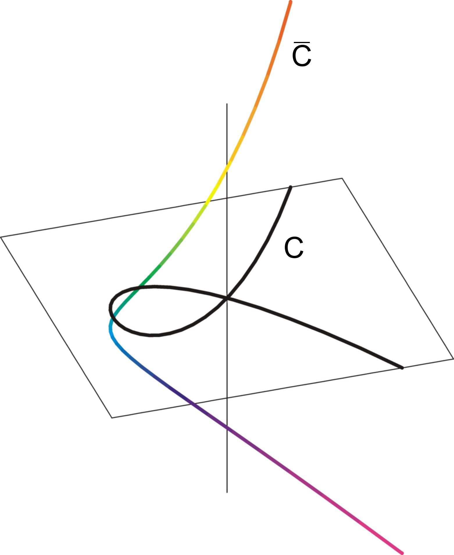
Figure 10. The normalization of the nodal plane curve $C=V(x^{3}+x^{2}-y^{2})$ is a variant of the twisted cubic curve $\overline{C}$ in 3-space.

Now, following [14], we describe how the normalization algorithm can be redesigned so that it becomes parallel in nature. For simplicity of the presentation, we focus on the case where $\operatorname{Sing}(A)$ is a finite set. This includes the case where $A$ is the coordinate ring of an algebraic curve.

In the example above, the curve under consideration has just one singularity. If there is a larger number of singularities, the normalization algorithm as discussed so far is global in the sense that it “improves” all singularities at the same time. Alternatively, we now aim at “improving” the individual singularities separately, and then put the individual results together. In this local-to-global approach, the local computations can be run in parallel. We make use of the following result.

Theorem 15 ([14]).

Suppose that $\operatorname{Sing}(A)=\{P_{1},\ldots,P_{r}\}$ is finite. Then:

1. For each $i$, let

   $$A\,\subseteq\,B_{i}\,\subseteq\,\overline{A}\vspace{-0.15cm}$$

   be the intermediate ring obtained by applying the normalization algorithm with $P_{i}$ in place of $J$. Then

   $$(B_{i})_{P_{i}} =\overline{A_{P_{i}}},\text{ and}$$

   $$(B_{i})_{Q} =A_{Q}\text{ for all }P_{i}\neq Q\in\operatorname{Spec}(A).\vspace{-0.15cm}$$

   We call $B_{i}$ the minimal local contribution to $\overline{A}$ at $P_{i}$.

2. We have

   $$\overline{A}=B_{1}+\ldots+B_{r}\text{.}$$

This theorem, together with the local version of the Grauert-Remmert criterion, whose proof is given in [14], yields an algorithm for normalization which is often considerably faster than the global algorithm presented earlier, even if the local-to-global algorithm is not run in parallel. The reason for this is that the cost for “improving” just one singularity is in many cases much less than that for “improving” all singularities at the same time. The new algorithm is implemented in the Singular library locnormal.lib [12]. Over the rationals, the algorithm becomes even more powerful by combining it with a modular approach. This version of the algorithm is implemented in the Singular library modnormal.lib [13].

4. Computing GIT-Fans

In this section, we give an example of an algorithm that uses Gröbner bases, polyhedral computations and algorithmic group theory. It is also suitable for parallel computations.

Recall that one of the goals of Geometric Invariant Theory (GIT) is to assign to a given algebraic variety $X$ that comes with the action of an algebraic group $G$ in a sensible manner a quotient space $X/\!\!/G$. This setting frequently occurs when we face a variety $X$ parameterizing a class of geometric objects, for example algebraic curves, and an action of a group $G$ on $X$ emerging from isomorphisms between the objects. There are two main problems. The first problem is that the homogeneous space $X/G$ is not a good candidate for $X/\!\!/G$ as it does not necessarily carry the structure of an algebraic variety. One then defines for affine $X$ the quotient $X/\!\!/G$ as the spectrum of the (finitely generated) invariant ring of the functions of $X$; for general $X$, one glues together the quotients of an affine covering. Now a second problem arises: the full quotient $X/\!\!/G$ may not carry much information: For instance, consider the action of $\mathbb{C}^{*}:=\mathbb{C}\setminus\{0\}$ on $X=\mathbb{C}^{2}$ given by component-wise multiplication

(1) $$\mathbb{C}^{*}\times X\,\to\,X,\qquad(t,(x,y))\,\mapsto\,(tx,ty).$$

Then the quotient $X/\!\!/\mathbb{C}^{*}$ is isomorphic to a point. However, considering the open subset $U:=X\setminus\{(0,0)\}$ gives us $U/\!\!/\mathbb{C}^{*}=\mathbb{P}^{1}$, the projective line. For general $X$, there are many choices for these open subsets $U\subseteq X$, where different choices lead to different quotients $U/\!\!/G$. To describe this behaviour, Dolgachev and Hu [26] introduced the GIT-fan, a polyhedral fan describing this variation of GIT-quotients. Recall that a polyhedral fan is a finite collection of strongly convex rational polyhedral cones such that their faces are again elements of the fan and the intersection of any two cones is a common face.

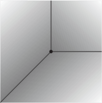
Figure 11. A polyhedral fan in $\mathbb{R}^{2}$.

Of particular importance is the action of an algebraic torus $G=(\mathbb{C}^{\ast})^{k}$, on an affine variety $X\subseteq\mathbb{C}^{r}$. In this case, Berchthold/Hausen and the third author [7, 44] have developed a method for computing the GIT-fan, see Algorithm 1. The input of the algorithm consists of

• an ideal $\mathfrak{a}\subseteq\mathbb{C}[T_{1},\ldots,T_{r}]$ which defines $X$ and

• a matrix $Q=(q_{1},\ldots,q_{r})\in\mathbb{Z}^{k\times r}$ such that $\mathfrak{a}$ is homogeneous with respect to the multigrading defined by setting $\deg(T_{i}):=q_{i}\in\mathbb{Z}^{k}$.

Note that the matrix $Q$ encodes the action of $(\mathbb{C}^{\ast})^{k}$ on $X$. For instance, the action (1) is encoded in $Q=(1,1)$.

Algorithm 1 can be divided into three main steps. For the first step, we decompose $\mathbb{C}^{r}$ into the $2^{r}$ disjoint torus orbits

$$\mathbb{C}^{r}\,=\,\bigcup_{\gamma\subseteq\{1,\ldots,r\}}\!\!O(\gamma),\qquad O(\gamma)\,:=\,\{(z_{1},\ldots,z_{r})\in\mathbb{C}^{r}\mid z_{i}\neq 0\Leftrightarrow i\in\gamma\}.$$

The algorithm then identifies in line 1 which of the torus orbits $O(\gamma)$ have a non-trivial intersection with $X$. The corresponding $\gamma\subseteq\{1,\ldots,r\}$ (interpreted as faces of the positive orthant $\mathbb{Q}_{\geq 0}^{r}$) are referred to as $\mathfrak{a}$-faces. Using the equivalence

$$X\cap O(\gamma)\,\neq\,\emptyset\quad\Longleftrightarrow\quad\left(\mathfrak{a}|_{T_{i}=0\text{ for }i\notin\gamma}\right):\langle T_{1}\cdots T_{r}\rangle^{\infty}\neq\langle 1\rangle,$$

the $\mathfrak{a}$-faces can be determined by computing the saturation through Gröbner basis techniques available in Singular. In the second step (line 2 of the algorithm), the $\mathfrak{a}$-faces are projected to cones in $\mathbb{Q}^{k}$. For each $\mathfrak{a}$-face $\gamma$, defining inequalities and equations of the resulting orbit cones

$$Q(\gamma):=\operatorname{cone}(q_{i}\mid i\in\gamma)\,\subseteq\,\Gamma:=\operatorname{cone}(q_{1},\ldots,q_{r})\,\subseteq\,\mathbb{Q}^{k}$$

are determined, where by $\operatorname{cone}(v_{1},\ldots,v_{k})$ we mean the polyhedral cone obtained by taking all non-negative linear combinations of the $v_{i}$. Computationally, this can be done via the double description method available in polymake. We denote by $\Omega$ the set of all orbit cones. In the final step, the GIT-fan is obtained as

$$\Lambda(\mathfrak{a},Q)\,:=\,\{\lambda_{\Omega}(w)\mid w\in\Gamma\}\quad\text{ where }\quad\lambda_{\Omega}(w)\,:=\,\bigcap_{w\in\eta\in\Omega}\eta.$$

To compute $\Lambda(\mathfrak{a},Q)$, we perform a fan-traversal in the following way: Starting with a random maximal GIT-cone $\lambda_{\Omega}(w_{0})\in\Lambda(\mathfrak{a},Q)$, we compute its facets, determine the GIT-cones $\lambda_{\Omega}(w)$ adjacent to it, and iterate until the support of the fan equals $\operatorname{cone}(q_{1},\ldots,q_{r})$. Figure 12 illustrates three steps in such a process.

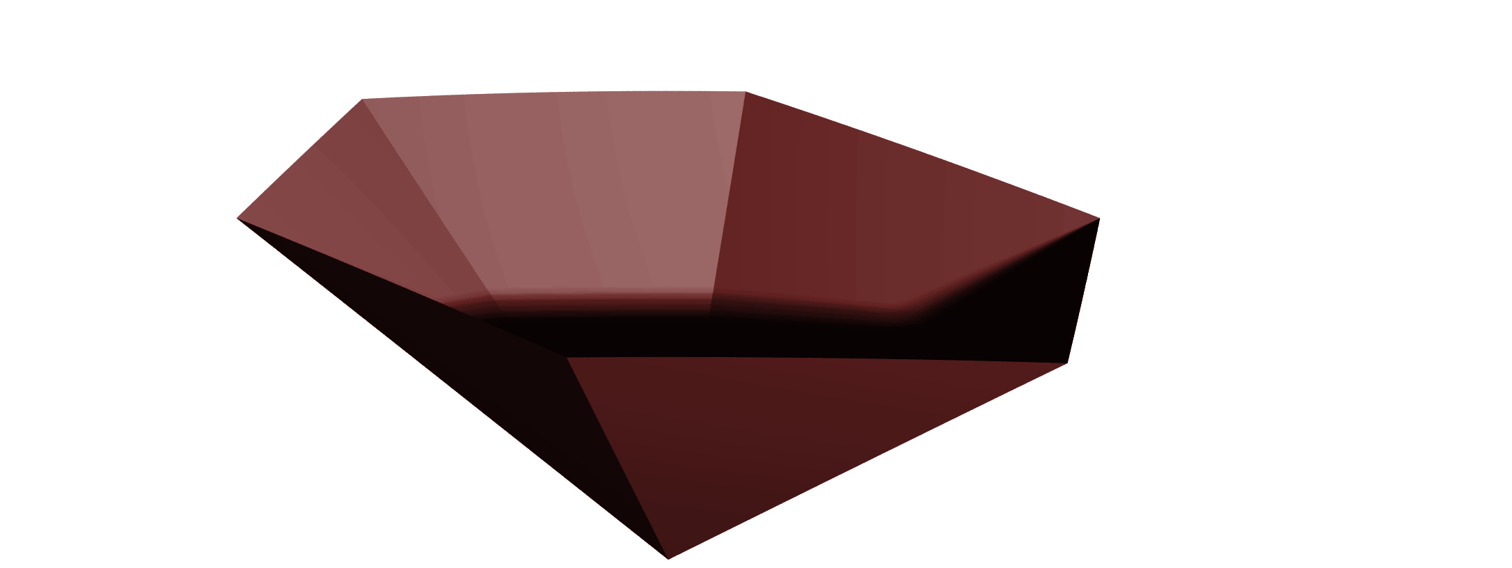
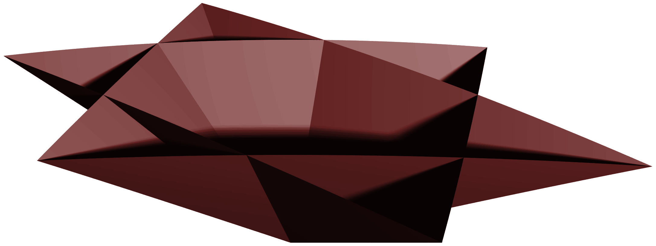
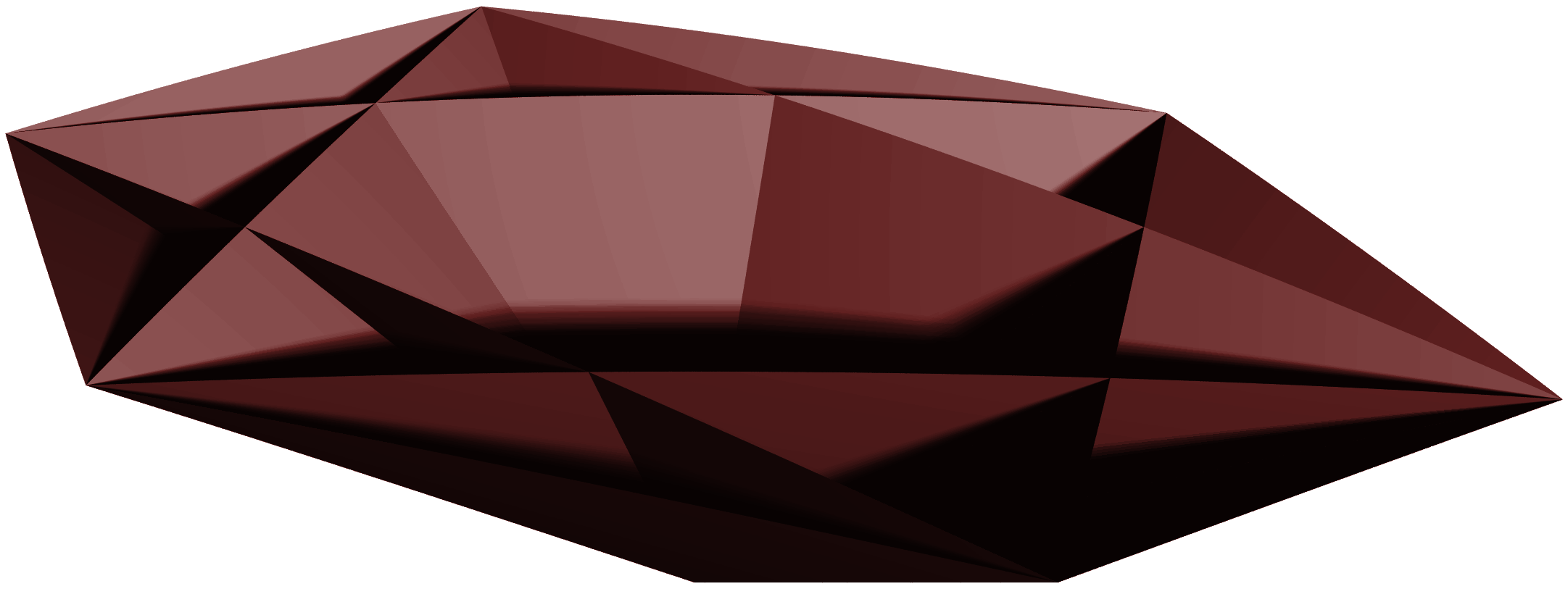
Figure 12. Fan traversal.

In line 9 of Algorithm 1, we write $\ominus$ for the symmetric difference in the first component. Again, computation of the facets of a given cone is available through the convex hull algorithms in polymake.

Algorithm 1 GIT-fan

0:  An ideal $\mathfrak{a}\subseteq\mathbb{C}[T_{1},\ldots,T_{r}]$ and a matrix $Q\in\mathbb{Z}^{k\times r}$ of full rank such that $\mathfrak{a}$ is homogeneous with respect to the multigrading given by $Q$.

0:  The set of maximal cones of $\Lambda(\mathfrak{a},Q)$.

1:  $\mathcal{A}:=\{\gamma\subseteq\mathbb{Q}_{\geq 0}^{r}\text{ face}\mid\gamma\text{ is an }\mathfrak{a}\text{-face}\}$

2:  $\Omega:=\left\{Q(\gamma)\mid\gamma\in\mathcal{A}\right\}$

3:  Choose a vector $w_{0}\in Q(\gamma)$ such that $\dim(\lambda_{\Omega}(w_{0}))=k$.

4:  $\mathcal{C}:=\{\lambda(w_{0})\}$

5:  $\mathcal{F}:=\{(\tau,\lambda_{\Omega}(w_{0}))\mid\tau\subseteq\lambda_{\Omega}(w_{0})\text{ facet with }\tau\not\subseteq\partial\Gamma\}$.

6:  while there is $(\eta,\lambda)\in\mathcal{F}$ do

7:     Find $w\in Q(\gamma)$ such that $w\not\in\lambda$ and $\lambda_{\Omega}(w)\cap\lambda=\eta$.

8:     $\mathcal{C}:=\mathcal{C}\cup\{\lambda_{\Omega}(w)\}$

9:     $\mathcal{F}:=\mathcal{F}\ominus\{(\tau,\lambda_{\Omega}(w))\mid\tau\subseteq\lambda_{\Omega}(w)\text{ facet with }\tau\not\subseteq\partial\Gamma\}$

10:  return  $\mathcal{C}$

Algorithm 1 is implemented in the Singular library gitfan.lib [16]. The Singular to polymake interface polymake.so [45] provides key convex geometry functionality in the Singular interpreter through a kernel level interface written in C++. We illustrate the use of this interface by a simple example.

Example 16.

We compute the normal fan $F$ of the Newton polytope $P$ of the polynomial $f=x^{3}+y^{3}+1$, see Figure 11. Note that $F$ is the Gröbner fan of the ideal $\langle f\rangle$ and its codimension one skeleton is the tropical variety of $\langle f\rangle$.

$\color[rgb]{0,0,1}>$ LIB "polymake.so";

Welcome to polymake version 2.14

Copyright (c) 1997-2015

Ewgenij Gawrilow, Michael Joswig (TU Berlin)

http://www.polymake.org

// ** loaded polymake.so

$\color[rgb]{0,0,1}>$ ring R = 0,(x,y),dp; poly f = x3+y3+1;

$\color[rgb]{0,0,1}>$ polytope P = newtonPolytope(f);

$\color[rgb]{0,0,1}>$ fan F = normalFan(P); F;

RAYS: -1 -1 #0  0  1 #1  1  0 #2 MAXIMAL_CONES: {0 1} #Dimension 2 {0 2} {1 2}

For many relevant examples, the computation of GIT-fans is challenged not only by the large amount of computations in lines 1 and 6 of Algorithm 1, but also by the complexity of each single computation in some boundary cases. Making use of symmetries and parallel computations, we can open up the possibility to handle many interesting new cases by considerably simplifying and speeding up the computations. For instance, the computations in line 1 of Algorithm 1 can be executed independently in parallel. Parallel computation techniques can also be applied in the computation of $\lambda_{\Omega}(w_{0})$ and the traversal of the GIT-fan. This step, however, is not trivially parallel.

An example of the use of symmetries is [17]; here, the first, third and fourth authors have applied and extended the technique described above to obtain the cones of the Mori chamber decomposition (the GIT-fan of the action of the characteristic torus on its total coordinate space) of the Deligne-Mumford compactification $\overline{M}_{0,6}$ of the moduli space of $6$-pointed stable curves of genus zero that lie within the cone of movable divisor classes. A priori, this requires to consider $2^{40}$ torus orbits in line 1. Hence, a direct application of Algorithm 1 in its stated form is not feasible. However, moduli spaces in algebraic geometry often have large amounts of symmetry. For example, on $\overline{M}_{0,6}$ there is a natural group action of the symmetric group $S_{6}$ which Bernal [8] has extended to the input data $\mathfrak{a}$ and $Q$ required for Algorithm 1. The GIT-fan $\Lambda(\mathfrak{a},Q)$, and all data that arises in its computation reflect these symmetries. Hence, by computing an orbit decomposition under the action of the group of symmetries of the set of all torus orbits, we can restrict ourselves to a distinct set of representatives. Also the fan-traversal can be done modulo symmetry. To compute the orbit decomposition, we apply the algorithms for symmetric groups implemented in GAP.

Example 17.

We apply this technique in the case of the affine cone $X$ over the Grassmannian $\mathbb{G}(2,5)$ of $2$-dimensional linear subspaces in a $5$-dimensional vector space, see also [17]. By making use of the action of $S_{5}$, the number of monomial containment tests in line 1 can be reduced from $2^{10}=1024$ to $34$. A distinct set of representatives of the orbits of the $172$ $\mathfrak{a}$-faces consists of $14$ elements. The GIT-fan has $76$ maximal cones, which fall into $6$ orbits. Figure 13 shows both the adjacency graph of the maximal cones of the GIT-fan and that of their orbits under the $S_{5}$-action. This GIT-fan has also been discussed in [8, 26, 2]. Note that by considering orbits of cones not only the computation of the fan is considerably simplified, but also the theoretical understanding of the geometry becomes easier.

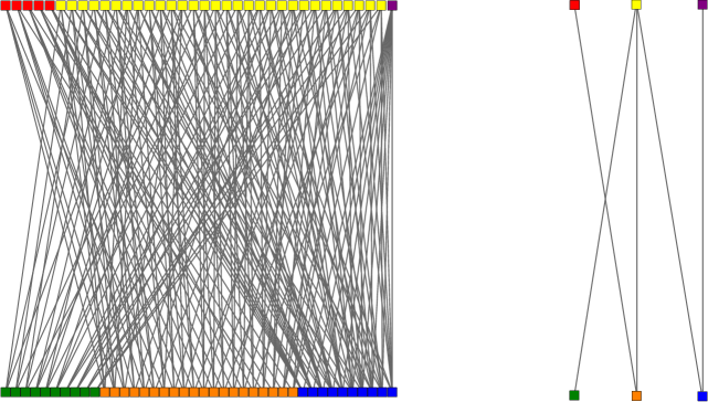
Figure 13. The adjacency graph of the set of maximal cones of the GIT-fan of $\mathbb{G}(2,5)$ and the adjacency graph of the orbits of these cones under the $S_{5}$-action.

To summarize, Algorithm 1 requires the following key computational techniques from commutative algebra, convex geometry, and group theory:

• Gröbner basis computations,

• convex hull computations, and

• orbit decomposition.

These techniques are provided by Singular, polymake, and GAP. At the current stage, polymake can be used from Singular in a convenient way through polymake.so. An interface to use GAP functionality directly from Singular is subject to future development.

References

- [1] E. A. Arnold. Modular algorithms for computing Gröbner bases. J. Symbolic Comput., 35(4):403–419, 2003.
- [2] I. V. Arzhantsev and J. Hausen. Geometric invariant theory via Cox rings. J. Pure Appl. Algebra, 213(1):154–172, 2009.
- [3] M. Barakat. Computations of unitary groups in characteristic . http://www.mathematik.uni-kl.de/~barakat/forJPSerre/UnitaryGroup.pdf, 2014.
- [4] R. Behrends. Shared memory concurrency for GAP. Computer Algebra Rundbrief, 55:27–29, 2014.
- [5] R. Behrends, K. Hammond, V. Janjic, A. Konovalov, S. Linton, H.-W. Loidl, P. Maier, and P. Trinder. HPC-GAP: engineering a 21st-century high-performance computer algebra system. Concurrency and Computation: Practice and Experience, 2016. cpe.3746.
- [6] R. Behrends, A. Konovalov, S. Linton, F. Lübeck, and M. Neunhöffer. Parallelising the computational algebra system GAP. In Proceedings of the 4th International Workshop on Parallel and Symbolic Computation, PASCO ’10, pages 177–178. ACM, New York, 2010.
- [7] F. Berchtold and J. Hausen. GIT equivalence beyond the ample cone. Michigan Math. J., 54(3):483–515, 2006.
- [8] M. M. Bernal Guillén. Relations in the Cox Ring of . PhD thesis, University of Warwick, 2012.
- [9] E. Bierstone and P. D. Milman. Canonical desingularization in characteristic zero by blowing up the maximum strata of a local invariant. Invent. Math., 128(2):207–302, 1997.
- [10] J. Böhm, W. Decker, S. Laplagne, and G. Pfister. Computing integral bases via localization and Hensel lifting. 2015. http://arxiv.org/abs/1505.05054.
- [11] J. Böhm, W. Decker, S. Laplagne, and G. Pfister. Local to global algorithms for the Gorenstein adjoint ideal of a curve. 2015. http://arxiv.org/abs/1505.05040.
- [12] J. Böhm, W. Decker, S. Laplagne, G. Pfister, A. Steenpaß, and S. Steidel. locnormal.lib – A Singular library for a local-to-global approach to normalization, 2013. Available in the Singular distribution, http://www.singular.uni-kl.de.
- [13] J. Böhm, W. Decker, S. Laplagne, G. Pfister, A. Steenpaß, and S. Steidel. modnormal.lib – A Singular library for a modular approach to normalization, 2013. Available in the Singular distribution, http://www.singular.uni-kl.de.
- [14] J. Böhm, W. Decker, S. Laplagne, G. Pfister, A. Steenpaß, and S. Steidel. Parallel algorithms for normalization. J. Symbolic Comput., 51:99–114, 2013.
- [15] J. Böhm, W. Decker, S. Laplagne, and F. Seelisch. paraplanecurves.lib – A Singular library for the parametrization of rational curves, 2013. Available in the Singular distribution, http://www.singular.uni-kl.de.
- [16] J. Böhm, S. Keicher, and Y. Ren. gitfan.lib – A Singular library for computing the GIT fan, 2015. Available in the Singular distribution, http://www.mathematik.uni-kl.de/~boehm/gitfan.
- [17] J. Böhm, S. Keicher, and Y. Ren. Computing GIT-fans with symmetry and the Mori chamber decomposition of , 2016. https://arxiv.org/abs/1603.09241.
- [18] D. K. Boku, W. Decker, C. Fieker, and A. Steenpass. Gröbner bases over algebraic number fields. In Proceedings of the 2015 International Workshop on Parallel Symbolic Computation, PASCO ’15, pages 16–24, New York, NY, USA, 2015. ACM.
- [19] W. Bosma, J. Cannon, and C. Playoust. The Magma algebra system. I. The user language. J. Symbolic Comput., 24(3-4):235–265, 1997. Computational algebra and number theory (London, 1993).
- [20] A. M. Bravo, S. Encinas, and O. Villamayor U. A simplified proof of desingularization and applications. Rev. Mat. Iberoamericana, 21(2):349–458, 2005.
- [21] W. Bruns and B. Ichim. Normaliz: algorithms for affine monoids and rational cones. J. Algebra, 324(5):1098–1113, 2010.
- [22] B. Buchberger. Ein Algorithmus zum Auffinden der Basiselemente des Restklassenringes nach einem nulldimensionalen Polynomideal. dissertation, Universität Innsbruck, 1965.
- [23] T. de Jong. An algorithm for computing the integral closure. J. Symbolic Comput., 26(3):273–277, 1998.
- [24] W. Decker, T. de Jong, G.-M. Greuel, and G. Pfister. The normalization: a new algorithm, implementation and comparisons. In Computational methods for representations of groups and algebras (Essen, 1997), volume 173 of Progr. Math., pages 177–185. Birkhäuser, Basel, 1999.
- [25] W. Decker, G.-M. Greuel, G. Pfister, and H. Schönemann. Singular 4-0-2 — A computer algebra system for polynomial computations. http://www.singular.uni-kl.de, 2015.
- [26] I. V. Dolgachev and Y. Hu. Variation of geometric invariant theory quotients. (With an appendix: “An example of a thick wall” by Nicolas Ressayre). Publ. Math., Inst. Hautes Étud. Sci., 87:5–56, 1998.
- [27] D. Eisenbud. Commutative algebra: With a view toward algebraic geometry, volume 150 of Graduate Texts in Mathematics. Springer-Verlag, New York, 1995.
- [28] D. Eisenbud. The geometry of syzygies, volume 229 of Graduate Texts in Mathematics. Springer-Verlag, New York, 2005. A second course in commutative algebra and algebraic geometry.
- [29] D. Eisenbud, G. Fløystad, and F.-O. Schreyer. Sheaf cohomology and free resolutions over exterior algebras. Trans. Am. Math. Soc., 355(11):4397–4426, 2003.
- [30] S. Encinas and H. Hauser. Strong resolution of singularities in characteristic zero. Comment. Math. Helv., 77(4):821–845, 2002.
- [31] B. Erocal, O. Motsak, F.-O. Schreyer, and A. Steenpass. Refined algorithms to compute syzygies. J. Symb. Comput, 74:308–327, 2016.
- [32] A. Frühbis-Krüger. Computational aspects of singularities. In Singularities in geometry and topology, pages 253–327. World Sci. Publ., Hackensack, NJ, 2007.
- [33] A. Frühbis-Krüger. resolve.lib – A Singular library for the resolution of singularities, 2015. Available in the Singular distribution, http://www.singular.uni-kl.de.
- [34] The GAP Group. GAP – Groups, Algorithms, and Programming, Version 4.7.9, 2015.
- [35] E. Gawrilow and M. Joswig. polymake: a framework for analyzing convex polytopes. In G. Kalai and G. M. Ziegler, editors, Polytopes — Combinatorics and Computation, pages 43–74. Birkhäuser, 2000.
- [36] H. Grauert and R. Remmert. Analytische Stellenalgebren. Springer-Verlag, Berlin-New York, 1971. Unter Mitarbeit von O. Riemenschneider, Die Grundlehren der mathematischen Wissenschaften, Band 176.
- [37] D. R. Grayson and M. E. Stillman. Macaulay2, a software system for research in algebraic geometry. Available at http://www.math.uiuc.edu/Macaulay2/.
- [38] G.-M. Greuel, S. Laplagne, and F. Seelisch. Normalization of rings. J. Symbolic Comput., 45(9):887–901, 2010.
- [39] G.-M. Greuel, S. Laplagne, and F. Seelisch. normal.lib – A Singular library for normalization, 2010. Available in the Singular distribution, http://www.singular.uni-kl.de.
- [40] S. Hampe. a-tint: a polymake extension for algorithmic tropical intersection theory. European J. Combin., 36:579–607, 2014.
- [41] B. Hart. ANTIC: Algebraic Number Theory in C. Computer Algebra Rundbrief, 56, 2015.
- [42] W. Hart, F. Johansson, and S. Pancratz. FLINT: Fast Library for Number Theory, 2013. Version 2.4.0, http://flintlib.org.
- [43] C. Huneke and I. Swanson. Integral closure of ideals, rings, and modules, volume 336 of London Mathematical Society Lecture Note Series. Cambridge University Press, Cambridge, 2006.
- [44] S. Keicher. Computing the GIT-fan. Internat. J. Algebra Comput., 22(7):1250064, 11, 2012.
- [45] Y. Ren. polymake.so – A Singular module for interfacing with polymake, 2015. Available in the Singular distribution, http://www.singular.uni-kl.de.
- [46] F.-O. Schreyer. Die Berechnung von Syzygien mit dem verallgemeinerten Weierstraßschen Divisionssatz und eine Anwendung auf analytische Cohen-Macaulay-Stellenalgebren minimaler Multiplizität. Diploma thesis, Universität Hamburg, 1980.
- [47] J.-P. Serre. Bases normales autoduales et groupes unitaires en caractéristique 2. Transform. Groups, 19(2):643–698, 2014.
- [48] A. Steenpaß. parallel.lib – A Singular library for parallel computations, 2015. Available in the Singular distribution, https://www.singular.uni-kl.de.
- [49] The homalg project authors. The project – Algorithmic Homological Algebra. http://homalg.math.rwth-aachen.de/, 2003–2014.