Structural Change in (Economic) Time Series

Abstract

Methods for detecting structural changes, or change points, in time series data are widely used in many fields of science and engineering. This chapter sketches some basic methods for the analysis of structural changes in time series data. The exposition is confined to retrospective methods for univariate time series. Several recent methods for dating structural changes are compared using a time series of oil prices spanning more than 60 years. The methods broadly agree for the first part of the series up to the mid-1980s, for which changes are associated with major historical events, but provide somewhat different solutions thereafter, reflecting a gradual increase in oil prices that is not well described by a step function. As a further illustration, 1990s data on the volatility of the Hang Seng stock market index are reanalyzed.

Keywords: change point problem, segmentation, structural change, time series.

JEL classification: C22, C87.

1 Introduction

In time series analysis, the point of reference is that of a stationary stochastic process; i.e., a process for which the sequence of first and second-order moments is constant (‘weak stationarity’), or even the sequence of the entire marginal distributions (‘strict stationarity’). In practice, many time series exhibit some form of nonstationarity: changing levels, changing variances, changing autocorrelations, or a combination of some or all of these aspects. These phenomena are then called structural changes or structural breaks and the associated statistical methodology is sometimes called change point analysis. Such phenomena may be seen as ‘complex’ in the sense of this Volume, in that classical models with constant coefficients are rejected by the data.

Structural change methodology is widely used in economics, finance, bioinformatics, engineering, public health, and climatology, to mention just a few fields of application. An interesting recent contribution (Kelly and Ó Gráda, 2014) disputes the existence of a ‘little ice age’ for parts of Central and Northern Europe between the 14th and 19th century. Using structural change methodology (of the type used below) on temperature reconstructions spanning several centuries, Kelly and Ó Gráda find no evidence for sustained falls in mean temperatures prior to 1900, instead several relevant series are best seen as white noise series. One explanation for the contradiction to the established view is the climatological practice of smoothing data prior to analysis. When the raw data are in fact uncorrelated, such preprocessing can introduce spurious dependencies (the ‘Slutsky effect’).

More than 25 years ago, a bibliography on structural change methodology and applications published in the economics literature (Hackl and Westlund, 1989) already lists some 500 references, and the literature has grown rather rapidly since then. More recently, a bibliography available with the R package strucchange provides more than 800 references, ending in 2006 (Zeileis et al., 2002). Recent surveys of the methodology include Perron (2006), Aue and Horváth (2013) and Horváth and Rice (2014). Much of this methodology relies quite heavily on functional central limit theorems (FCLTs), an excellent reference is Csörgő and Horváth (1997).

Apart from practical relevance of the associated issues, one reason for the large number of publications is that the notion of ‘structural change’ can be formalized in many different ways. In terms of statistical hypothesis tests, the null hypothesis of ‘no structural change’ is reasonably clear (model parameters are constant), but the alternative can mean many things: a parameter (or several parameters) change(s) its (their) value(s) abruptly (once, twice, or more often), or it changes gradually according to a stochastic mechanism (e.g., via a random coefficient model), or it switches randomly among a small number of states (e.g., via a hidden Markov model), etc. There are many further possibilities.

The available methodology therefore incorporates ideas from a variety of fields: linear models, sequential analysis, wavelets, etc. In economics, there is comparatively greater interest in changes in regression models, whereas in many other fields of application interest is focused on changes in a univariate time series. A further dividing line is on-line (sequential) analysis of a growing sample vs. off-line (retrospective) analysis of a fixed sample.

This chapter provides some basic ideas of change point methodology along with empirical examples. It is biased towards least-squares methods, methodology used in economics and finance as well as availability in statistical software. The following section outlines selected methods in the context of a simple signal-plus-noise model. For reasons of space, the exposition is confined to retrospective analysis of changes in univariate time series. In section 3, several recent algorithms are explored for dating structural changes in a series of oil prices. Section 4 dates volatility changes in Hang Seng stock market index returns, thereby revisiting data formerly studied in Andreou and Ghysels (2002). The final section provides some references for sequential analysis of structural change and also for more complex data structures.

2 Some basic ideas in change point analysis

To fix ideas, consider a signal-plus-noise model for an observable (univariate) quantity $y_{i}$,

$$y_{i}\leavevmode\nobreak\ =\leavevmode\nobreak\ \mu_{i}+e_{i},\quad i=1,\dots,T,$$

where $\mu_{i}$ is the (deterministic) signal and $e_{i}$ is the noise, with $\mbox{{E}}[e_{i}]=0$ and $\mbox{{Var}}[e_{i}]=\sigma^{2}$. As noted above, this chapter is confined to changes in a univariate time series. However, for many methods, there is a regression version with $\mu_{i}=x_{i}^{\top}\beta_{i}$, where $x_{i}$ is a vector of covariates and $\beta_{i}$ the corresponding set of regression coefficients. In the classical setting, the $e_{i}$ form a sequence of independent and identically distributed (i.i.d.) random variables, but many more recent contributions, especially in economics and finance, consider dependent processes.

2.1 Testing for structural change

In terms of statistical testing, the null hypothesis of interest is $H_{0}:\mu_{i}=\mu_{0}$ for all $i$; i.e., the signal exhibits no change. (For the regression version, the corresponding null hypothesis is $H_{0}:\beta_{i}=\beta_{0}$ for all $i$.) Under the null hypothesis, natural estimates of $\mu_{0}$ are the recursive estimates $\hat{\mu}_{k}=k^{-1}\sum_{i=1}^{k}y_{i}$, $k=1,\dots,T$; i.e., the sequence of sample means computed from a growing sample. The corresponding recursive residuals are $\tilde{e}_{i}=y_{i}-\hat{\mu}_{i-1}$, $i=2,\dots,T$.

A classical idea is to study the fluctuations of partial (or cumulative) sums (CUSUMs) of these recursive residuals and to reject the null hypothesis of parameter stability if their fluctuations are excessive. In order to assess significance, introduce an empirical fluctuation process indexed by $t\in[0,1]$ as the process of partial sums of the recursive residuals via

$$\tilde{S}_{T}(t)\leavevmode\nobreak\ =\leavevmode\nobreak\ \frac{1}{\hat{\sigma}_{T}\sqrt{T}}\sum_{i=1}^{[Tt]}\tilde{e}_{i},\quad 0\leq t\leq 1,$$

where $[Tt]$ denotes the integer part of $Tt$ and $\hat{\sigma}_{T}^{2}$ some consistent estimate of $\sigma^{2}$. This object is often called the Rec-CUSUM process as it is based on recursive residuals. It is well known that under the above assumptions this empirical fluctuation process can be approximated by a Brownian motion, $B(t)$, $0\leq t\leq 1$, and hence the enormous literature on properties of this stochastic process can be used to assess the fluctuations in the recursive residuals. Excessive fluctuation is determined from the crossing probabilities of certain boundaries, this is the approach proposed in the seminal paper by Brown et al. (1975).

However, from a regression point of view, the ordinary least-squares (OLS) residuals $\hat{e}_{i}=y_{i}-\hat{\mu}_{T}$ are perhaps a more natural starting point, leading to the test statistic

$$\max_{k=1,\dots,T}\left|\frac{1}{\hat{\sigma}_{T}\sqrt{T}}\sum_{i=1}^{k}\hat{e}_{i}\right|.$$ (1)

As OLS residuals are correlated and sum to zero by construction, the limiting process corresponding to the OLS-CUSUM process is no longer a Brownian motion. Instead, the limiting process is now a Brownian bridge, $B^{0}(t)$, with $B^{0}(t)=B(t)-t\leavevmode\nobreak\ B(1)$, $0\leq t\leq 1$, and the relevant limiting quantity for assessing significant deviation from the null hypothesis is

$$\sup_{0\leq t\leq 1}|B^{0}(t)|,$$

the supremum of the absolute value of a Brownian bridge on the unit interval (Ploberger and Krämer, 1992). This object is well known in the statistical literature, and quantiles of its distribution provide critical values for a test based on (1).

To briefly illustrate the machinery, consider a time series of measurements of the annual flow of the river Nile at Aswan, for the period 1871 to 1970. This series is part of any binary distribution of R (R Core Team, 2016) under the name Nile and has been used repeatedly in the statistical literature on change point methods. The following illustrations make use of the R package strucchange, which among other things implements structural change detection using empirical fluctuation processes and related techniques. It should be noted that the original paper (Zeileis et al., 2002) describing the software documents the first release of the package, but many methods were added in subsequent years, including the methods for dating structural changes that are used in the next section. The package is still actively maintained, but the main developments happened some 10 years ago.

Figure 1 plots the time series (left panel) and the corresponding OLS-CUSUM process (right panel) along with a boundary indicating the 5% critical value for the test statistic (1). It is seen that the empirical fluctuation process crosses the boundary, and hence the hypothesis of a constant level is rejected at the 5% level.

Figure 1: Nile river discharges: Raw data (left) and OLS-CUSUM process (right).

The test statistic (1), often called the OLS-CUSUM test, measures the maximal absolute deviation from zero of the corresponding OLS-CUSUM process. There are many variations of this idea. For example, it is possible to use other functionals of the empirical fluctuation process, such as the range or some average of the fluctuations. It is also possible to study moving instead of cumulative sums, leading to moving sum (MOSUM) processes. Or, instead of the fluctuations in the residuals, one can directly assess the fluctuations in the estimates themselves; there are again recursive and moving versions (Kuan and Hornik, 1995). In the univariate case considered here, the latter idea is equivalent to CUSUMs or MOSUMs of the residuals, but in the regression case it leads to new procedures. It is also possible to assess fluctuations in first-order conditions of fitting methods other than least squares, for example likelihood methods (Zeileis, 2005).

Also, applications in economics and finance often involve dependent data, so that the machinery described above requires adjustments. These involve the long-run variance,

$$\omega^{2}\leavevmode\nobreak\ =\leavevmode\nobreak\ \lim_{T\to\infty}\mbox{{Var}}(\tilde{S}_{T}(1)).$$

If a consistent estimator $\hat{\omega}^{2}$ of $\omega^{2}$ is available, then $\hat{\omega}^{-1}\tilde{S}_{T}(t)$ or $\hat{\omega}^{-1}\hat{S}_{T}(t)$ can, in many settings of interest, again be approximated by a Brownian motion or a Brownian bridge.

2.2 Dating structural changes

Having found evidence for the presence of structural change it is of interest to estimate the change points themselves. In economics, basic references for dating structural changes are Bai and Perron (1998, 2003), which among other things provide a method for obtaining confidence intervals for the break dates. The associated point estimation issue – the segmentation of the sample into homogeneous parts – dates back at least to Bellman and Roth (1969).

The model of interest is now a step function for the signal. With $m+1$ segments (corresponding to $m$ breaks), this is

$$y_{i}\leavevmode\nobreak\ =\leavevmode\nobreak\ \mu_{j}+e_{i},\qquad\tau_{j-1}+1\leavevmode\nobreak\ \leq\leavevmode\nobreak\ i\leavevmode\nobreak\ \leq\leavevmode\nobreak\ \tau_{j},\quad j=1,\dots,m+1.$$ (2)

Here $j$ is the segment index and $\{\tau_{1},\dots,\tau_{m}\}$ denotes the set of the break points. By convention, $\tau_{0}=0$ and $\tau_{m+1}=T$.

Given the break points $\tau_{1},\dots,\tau_{m}$, the least squares estimate of $\mu_{j}$ is the sample mean of the observations pertaining to segment $j$. The resulting aggregate residual sum of squares is given by

$$RSS(\tau_{1},\dots,\tau_{m})\quad=\quad\sum_{j=1}^{m+1}rss(\tau_{j-1}+1,\tau_{j}),$$ (3)

where $rss(\tau_{j-1}+1,\tau_{j})$ is the residual sum of squares for segment $j$. The problem of dating structural changes is to find the break points $\hat{\tau}_{1},\dots,\hat{\tau}_{m}$ that minimize the objective function,

$$\{\hat{\tau}_{1},\dots,\hat{\tau}_{m}\}\quad=\quad\mbox{argmin}_{\{\tau_{1},\dots,\tau_{m}\}}RSS(\tau_{1},\dots,\tau_{m}),$$ (4)

over all partitions $\{\tau_{1},\dots,\tau_{m}\}$ with $\tau_{j}-\tau_{j-1}\geq T_{\min}$. Here $T_{\min}$ is a bandwidth parameter to be specified by the user, it defines the minimal segment length. For a given number $m$ of break points, their optimal location can be found using a dynamic programming algorithm. The number of change points $m$ itself can be determined via information criteria, the breakpoints() function in strucchange employs the Bayesian Information Criterion (BIC). Below, this algorithm is referred to as breakpoints. More details on the implementation may be found in Zeileis et al. (2003).

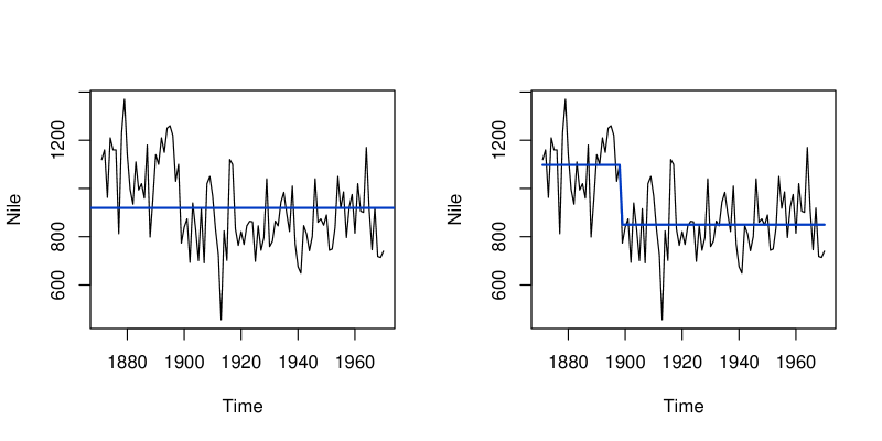
Figure 2: Nile river discharges: Model with constant level (left) vs. model with two regimes (right).

Returning to the Nile river flows, Figure 2 (left panel) provides the fit for a traditional autoregressive model of order one (AR(1)) with constant parameters. Clearly, the fit is quite poor in that for the first part of the series the data are almost always above the fitted mean level, whereas after approximately the year 1900 they are mostly below. In contrast, Figure 2 (right panel) provides a model with a changing level, the BIC suggesting a model with a single break corresponding to the year 1898. There is a simple explanation for this break: the opening of the Aswan dam in 1898. It is worth noting that after modelling the break there is no need for further modelling of any dependence about the changing level: the dependence implied by the fitted AR(1) process (left panel), with an autoregressive parameter of $0.51$, is spurious and stems from the neglected data feature of a changing level.

3 Dating changes in a commodity price series

This section revisits an empirical example presented in Zeileis et al. (2003), namely dating structural breaks in a time series of oil prices. That paper considered a quarterly index of import prices of petroleum products obtained from the German Federal Statistical Office – hereafter referred to as the German oil price data – for the period 1960(1) to 1994(4) (base year: 1991). The present paper uses a much longer series, a quarterly time series of spot prices for West Texas Intermediate (WTI) – hereafter referred to as the WTI data – from 1947(1) to 2013(3). It is publicly available from the FRED database of the Federal Reserve Bank of St. Louis, more specifically from https://research.stlouisfed.org/fred2/series/OILPRICE/. The series is deflated using the GDP deflator (base year: 2009), which is available from https://research.stlouisfed.org/fred2/series/GDPDEF/. This deflated version is given in Figure 3 (data are in logarithms). The task is to compare a change point model for the WTI data with the corresponding segmentation for the older German oil price data, and also to try out several more recent dating algorithms, on which more below.

Figure 3: Quarterly spot prices for West Texas Intermediate (WTI). Source: Federal Reserve Bank of St. Louis (FRED databse).

For ease of reference, the older series along with a segmentation with three regimes is given in Figure 4 (data are again in logarithms). The three breaks are for the quarters 1973(3), 1979(1) and 1985(1). The first two breaks correspond to two major historical events, the first oil crisis (the Arab oil embargo following the Yom Kippur war) and the beginning of the Iranian revolution. The break in 1985(1) may be seen as resulting from demand shifts, quarrels within OPEC, and the entry of several new suppliers (namely Great Britain, Mexico, and Norway) in international oil markets (Zeileis et al., 2003).

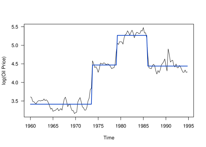
Figure 4: German oil price data, 1960(1) to 1994(4) (base year: 1991). Data source: German Federal Statistical Office. Segmentation as in Zeileis et al. (2003).

Repeating the exercise with the newer WTI data and a minimal segment size of 10 quarters, the BIC now favors a segmentation with 10 regimes. The resulting solution is provided in the second panel of Figure 5. There is good agreement for the breaks corresponding to major historical events, here estimated at 1973(4) and 1979(2). Beginning in the second half of the 1990s, there is a gradual trend in the newer series that is not described well by a step function. Also, the two oil price series differ visibly in the first half of the 1980s, leading to two estimated change points for the newer series, at 1982(4) and 1985(4). These differences result from the fact that the older series is a price index while the newer is for a single product; also, there appear to be exchange rate effects in the older series.

We next compare the least-squares-based solution with two recent methods. The first method (Matteson and James, 2014) uses ideas from cluster analysis combined with a nonparametric form of ANOVA based on so-called energy statistics (Rizzo and Székely, 2010). The latter are functions of distances between statistical observations in Euclidean spaces (and beyond), the name derives from an analogy with Newton’s gravitational potential energy. It should be noted that this method assesses differences in entire distributions, not just level shifts. However, there is a variant that assesses only changes in the mean; the relevant settings for this variant are used below. An implementation is available in the R package ecp (James and Matteson, 2014). The package offers several methods, here only the algorithm named e.divisive there is used, a form of hierarchical clustering. The second method is wild binary segmentation (Fryzlewicz, 2014) (hereafter: WBS), a stochastic algorithm that uses ideas from the wavelets literature. The setup analyzed in the original paper is (2) with i.i.d. Gaussian noise. An implementation is available in the R package wbs.

All three procedures require specification of a trimming parameter, for the least-squares approach and e.divisive this is the minimal segment length (or ‘cluster size’, in the terminology of the ecp package), details differ from method to method. For e.divisive, the minimal segment size was again set to 10 quarters, here yielding 9 breaks. For WBS, which does not need a minimal segment size, the maximum number of breaks was fixed at 10 for comparability reasons. The solutions are provided in the third and fourth panel of Figure 5. There is good agreement for the major historical events, while the algorithms differ somewhat for the second half of the series. This partly reflects the problems with this part of the series mentioned above. Overall, WBS tries to adapt to smaller details towards the end of the series. It is also worth noting that, using the settings recommended by the authors of the software, the WBS algorithm favors a solution with no fewer than 35 breaks. Clearly, not all of the estimated breaks will be of economic interest. This appears to be a problem in some financial applications, where alarms can be frequent with long series. As an example, not all changes identified in Fryzlewicz (2014) for the S&P 500 index will likely be of practical relevance.

Figure 5 provides an overall comparison of all solutions. The display highlights similarities and differences of the solutions obtained from the algorithms. Notably the breakpoints and e.divisive solutions are very similar. In contrast, wbs is more faithful to the more lively part towards the end of the series. breakpoints has one further change point in the second half of the 1990s (namely for the quarter 1997(1)), the other breaks differ, with one exception, by at most two quarters. For example, the break corresponding to the first oil crisis is in 1973(4) according to breakpoints and in 1974(1) according to e.divisive. For the Iranian revolution break, the algorithms give 1979(2) and 1979(4), respectively.

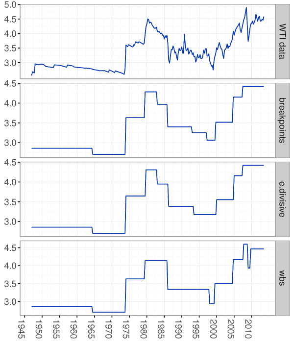
Figure 5: WTI data (top panel) and segmentations obtained from three algorithms: breakpoints, e.divisive and wbs.

4 Dating changes in the volatility of a stock market index

The previous section considered changes in the mean of a time series. It is also possible to study changes in other characteristics of the data, for example variances or autocorrelations. With financial time series, for example stock returns, assessing risks is a central issue; both squared and absolute returns may be seen as measures of risk. Assessing changes in such transformed returns can be viewed as an indirect check of structural change in GARCH-type models of volatility.

As a brief empirical illustration, we revisit an example from Andreou and Ghysels (2002). They consider four stock market indices (FTSE, Hang Seng, Nikkei, S&P500) with an eye on changes associated with the Asian and Russian financial crises in the second half of the 1990s. Here we just consider one of these series, the Hang Seng index for the period 1989–01–04 to 2001–10–19, giving $T=3338$ observations. For comparability reasons, the data are taken from Datastream. The data for the segmentation algorithm are the Hang Seng absolute returns (for which more breaks are found than for the more common squared returns). The original paper documents only the maximal number of breaks used but not the minimal segment size. Here we use a minimal segment size corresponding to 10% of the length of the series, which should permit recovery of the segmentation from Andreou and Ghysels (2002). This is only partly possible, however.

Figure 6 provides a plot of the absolute returns along with two models. The original paper suggests that a segmentation with three breaks, for the dates 1992-07-03, 1995-01-24 and 1997-08-15, is optimal. The 3-breaks solution found by breakpoints (the dashed line in the plot) differs, it finds 1995-06-14, 1997-08-15 and 1998-11-30, so only the last break from the paper is recovered. Also, the breakpoints solution has no break prior to 1995 but a new break after 1997.

It is also worth noting that the method finds a further break upon increasing the maximum number of breaks. Setting the latter to five breaks, a segmentation with four breaks is found. Interestingly, the new break at 1993-10-01 is before 1995, although not overly close to the 1992-07-03 break of Andreou and Ghysels (2002). Further experiments with the minimal segment length (down to 5% of the length of the series) and the admissible number of breaks (up to 10) suggest that the results are quite sensitive to the settings of these parameters. The only break that is practically always found is for August 1997, it is often estimated at 1997-08-15 and is associated with the Asian financial crisis.

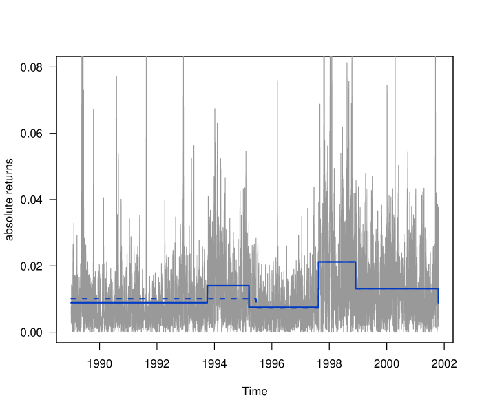
Figure 6: Segmentation of Hang Seng absolute returns with breakpoints. Dashed line: maximal number of breaks 3, minimal segment size 10%. Solid line: maximal number of breaks 5, minimal segment size 10%.

5 Discussion and outlook

This chapter has illustrated some basic ideas in change point analysis. The exposition was confined to retrospective methods for univariate time series. (Most of) The methods described have extensions to regression models (Perron, 2006). Many further topics had to be excluded, notably the timely topic of on-line monitoring and also structural change in multivariate or functional data. For on-line monitoring, in some fields referred to as surveillance or ‘quickest detection’ problems, see the survey by Frisén (2009) and references therein, for an exposition of associated optimality issues in a financial setting see Shiryaev (2002). Multivariate and functional data are briefly addressed in the recent survey by Horváth and Rice (2014), where further references may be found.

The literature will likely continue to grow rapidly, for several reasons: The classical methods are largely confined to linear models fitted via least squares methods. Nonlinear models for discrete-valued data are needed in some applications, but here the literature is still relatively small. Also, the growing number of large data sets demands improvements on the algorithmic side. Unfortunately, many recent methods are not readily available in statistical software, which to some extent hinders progress. A further big challenge is the unification of this widely scattered literature.

Computational Details

All results were obtained using R 3.2.4, with the packages strucchange 1.5-1, ecp 2.0.0, and wbs 1.3, on PCs running Mac OS X, version 10.10.5. Some plots were drawn using the package ggplot2 2.1.0 (Wickham, 2009).

References

- Andreou and Ghysels (2002) Andreou, E. and Ghysels, E. (2002). Detecting multiple breaks in financial market volatility dynamics. Journal of Applied Econometrics, 17 579–600.
- Aue and Horváth (2013) Aue, A. and Horváth, L. (2013). Structural breaks in time series. Journal of Time Series Analysis, 34 1–16.
- Bai and Perron (1998) Bai, J. and Perron, P. (1998). Estimating and testing linear models with multiple structural changes. Econometrica, 66 47–78.
- Bai and Perron (2003) Bai, J. and Perron, P. (2003). Computation and analysis of multiple structural change models. Journal of Applied Econometrics, 18 1–22.
- Bellman and Roth (1969) Bellman, R. and Roth, R. (1969). Curve fitting by segmented straight lines. Journal of the American Statistical Association, 64 1079–1084.
- Brown et al. (1975) Brown, R. L., Durbin, J. and Evans, J. M. (1975). Techniques for testing the constancy of regression relationships over time. Journal of the Royal Statistical Society B, 37 149–163.
- Csörgő and Horváth (1997) Csörgő, M. and Horváth, L. (1997). Limit Theorems in Change-Point Analysis. John Wiley & Sons.
- Frisén (2009) Frisén, M. (2009). Optimal sequential surveillance for finance, public health, and other areas. Sequential Analysis, 28 310–337.
- Fryzlewicz (2014) Fryzlewicz, P. (2014). Wild binary segmentation for multiple change-point detection. Annals of Statistics, 42 2243–2281.
- Hackl and Westlund (1989) Hackl, P. and Westlund, A. (1989). Statistical analysis of “structural change”: An annotated bibliography. Empirical Economics, 14 167–192.
- Horváth and Rice (2014) Horváth, L. and Rice, G. (2014). Extensions of some classical methods in change point analysis. TEST, 23 219–255.
- James and Matteson (2014) James, N. A. and Matteson, D. S. (2014). ecp: An R package for nonparametric multiple change point analysis of multivariate data. Journal of Statistical Software, 62 1–25. URL http://www.jstatsoft.org/v62/i07/.
- Kelly and Ó Gráda (2014) Kelly, M. and Ó Gráda, C. (2014). Change points and temporal dependence in reconstructions of annual temperature: Did Europe experience a Little Ice Age? Annals of Applied Statistics, 8 1372–1394.
- Kuan and Hornik (1995) Kuan, C.-M. and Hornik, K. (1995). The generalized fluctuation test: A unifying view. Econometric Reviews, 14 135–161.
- Matteson and James (2014) Matteson, D. S. and James, N. A. (2014). A nonparametric approach for multiple change point analysis of multivariate data. Journal of the American Statistical Association, 109 334–345.
- Perron (2006) Perron, P. (2006). Dealing with structural breaks. In Palgrave Handbook of Econometrics, Vol. 1: Econometric Theory (K. Patterson and T. C. Mills, eds.). Palgrave Macmillan, 278–352.
- Ploberger and Krämer (1992) Ploberger, W. and Krämer, W. (1992). The CUSUM test with OLS residuals. Econometrica, 60 271–285.
- R Core Team (2016) R Core Team (2016). R: A Language and Environment for Statistical Computing. R Foundation for Statistical Computing, Vienna, Austria. URL http://www.R-project.org/.
- Rizzo and Székely (2010) Rizzo, M. L. and Székely, G. J. (2010). DISCO analysis: A nonparametric extension of analysis of variance. Annals of Applied Statistics, 4 1034–1055.
- Shiryaev (2002) Shiryaev, A. N. (2002). Quickest detection problems in the technical analysis of financial data. In Mathematical Finance – Bachelier Congress 2000: Selected Papers from the First World Congress of the Bachelier Finance Society, Paris, June 29 – July 1, 2000 (H. Geman, D. Madan, S. Pliska and T. Vorst, eds.). Springer, 487–521.
- Wickham (2009) Wickham, H. (2009). ggplot2: Elegant Graphics for Data Analysis. Springer-Verlag, New York.
- Zeileis (2005) Zeileis, A. (2005). A unified approach to structural change tests based on ML scores, statistics, and OLS residuals. Econometric Reviews, 24 445–466.
- Zeileis et al. (2003) Zeileis, A., Kleiber, C., Krämer, W. and Hornik, K. (2003). Testing and dating of structural changes in practice. Computational Statistics & Data Analysis, 44 109–123.
- Zeileis et al. (2002) Zeileis, A., Leisch, F., Hornik, K. and Kleiber, C. (2002). strucchange: An R package for testing for structural change in linear regression models. Journal of Statistical Software, 7 1–38. URL http://www.jstatsoft.org/v07/i02/.