A Bayesian framework for distributed estimation
of arrival rates in asynchronous networks

Abstract

In this paper we consider a network of agents monitoring a spatially distributed arrival process. Each node measures the number of arrivals seen at its monitoring point in a given time-interval with the objective of estimating the unknown local arrival rate. We propose an asynchronous distributed approach based on a Bayesian model with unknown hyperparameter, where each node computes the minimum mean square error (MMSE) estimator of its local arrival rate in a distributed way. As a result, the estimation at each node “optimally” fuses the information from the whole network through a distributed optimization algorithm. Moreover, we propose an ad-hoc distributed estimator, based on a consensus algorithm for time-varying and directed graphs, which exhibits reduced complexity and exponential convergence. We analyze the performance of the proposed distributed estimators, showing that they: (i) are reliable even in presence of limited local data, and (ii) improve the estimation accuracy compared to the purely decentralized setup. Finally, we provide a statistical characterization of the proposed estimators. In particular, for the ad-hoc estimator, we show that as the number of nodes goes to infinity its mean square error converges to the optimal one. Numerical Monte Carlo simulations confirm the theoretical characterization and highlight the appealing performances of the estimators.

I Introduction

Arrival processes provide a useful description for events occurring with some probability in a given time or space interval. Applications range from communications and transports to medicine (e.g., diagnostic imaging) and astronomy (e.g., particle detection), [2]. From a statistical point of view the prominent model for arrival processes is notoriously Poisson. Indeed, even when independence between arrivals cannot be assumed, the superposition of a large number of non-Poisson processes is approximately distributed as a Poisson (Palm-Khintchine Theorem), [3]. Also, the limit distribution of counting processes described by the Binomial distribution is a Poisson, according to the law of rare events.

In modern network contexts (as, e.g., data, communication and sensor networks or Intelligent Transportation Systems) estimating the process intensity at different locations, i.e., the arrival rates at different nodes, is an important preliminary problem to be solved in order to gain context awareness. Clearly, each arrival rate can be estimated by performing a decentralized Maximum Likelihood (ML) estimation based only on the local arrivals at the given node. In this paper we want to investigate how the estimation can be improved by exploiting the cooperation among the nodes. Recently, a great interest has been devoted to cooperation schemes in which estimation is performed by a network of computing nodes in a distributed way, rather than by collecting all the data in a central unit, [4, 5, 6]. How to use the information from other nodes in the network and how to design a distributed algorithm merging such information will be the focus of the paper.

Distributed estimation has received a widespread attention in the distributed computation literature, especially as a natural application of linear (average) consensus algorithms, see, e.g. [7], or the recent surveys [8, 9]. Nodes typically interact iteratively with their neighbors by means of a “diffusion-like” process in which the estimation is improved by suitably combining the estimations from neighboring nodes, [6, 10, 11]. An incremental and a diffusive distributed algorithm with finite time convergence are proposed in [12] for (static) state estimation. Distributed optimization is also strictly related to distributed estimation. In [5] a distributed Alternating Direction Method of Multipliers (ADMM) has been introduced as a tool for distributed ML estimation of vector parameters in a wireless sensor network. Notice that ADMM and other distributed optimization algorithms, as, e.g., [13], can be used as building blocks to solve parts of an estimation problem in a distributed set-up. ML approaches for distributed estimation of a commonly observed parameter have been proposed also in [14]. In [15, 16] consensus-based algorithms have been developed to simultaneously estimate a common parameter measured by noisy sensors and classify sensor types. In [17] consensus-based algorithms have been developed to estimate global parameters in a linear Bayesian framework. In [18] a distributed algorithm is proposed for adaptive Bayesian estimation of a common parameter with known prior. Dynamic methods have been also proposed in which the nodes keep collecting new measurements while interacting with each other. In [19] a diffusion-based Recursive Least Squares (RLS) algorithm is proposed to estimate a constant parameter, but with dynamically acquired measurements. Finally, in [20] and [21] distributed ADMM-based algorithms are proposed for the estimation of random signals and dynamical processes.

Differently from the above references, in our work we consider a more general Bayesian framework that allows the nodes to improve their local estimate, rather than reaching a consensus on a common parameter. As detailed later, we will consider a special model for continuous mixtures of Poisson variables. Poisson mixtures have been widely used in the arrival-rate estimation literature to model non-homogeneous scenarios, see, e.g., [22, 23] as early references. The survey [24] provides an extensive review of properties and applications for Poisson mixtures. In a Bayesian setting the classical mixing (prior) distribution is the Gamma [24, 25], which results in a closed-form posterior [26].

The main contribution of the paper is twofold. First, we propose a distributed estimation scheme for arrival rates in an asynchronous network, based on a hierarchical probabilistic framework. Specifically, we develop an Empirical Bayes approach, in which the arrival rates are treated as random variables, whose prior distribution is parametrized by an unknown hyperparameter to be determined via ML estimation. In particular, we borrow from the centralized statistics literature the classical Gamma-Poisson model (for Poisson mixtures), assuming however the hyperparameter is unknown, and extend it to a scenario with non-homogeneous sample sizes. We show that the ML estimation of the hyperparameter is a separable optimization problem, that can be solved in a distributed way over the network by using a distributed optimization algorithm. Thanks to this modeling idea, the local estimates are obtained by taking advantage of the whole network data, thus improving the accuracy especially when the amount of local data is scarce. With this approach we are able to capture the fact that arrival rates are not the outcomes of isolated phenomena, but rather the expression of global properties of the process. For this “optimal” estimator we characterize mean and variance at steady-state (i.e., once agents have reached consensus on the optimal solution) for networks with a large number of agents.

Second, we propose an alternative ad-hoc distributed estimator that, although suboptimal, performs comparably to the optimal one. The main advantage of this ad-hoc estimator is that the resulting algorithm has a simple update rule based on linear consensus protocols, thus exhibiting the same appealing exponential convergence. For the ad-hoc estimator we also characterize transient (at any time-instant) mean and variance for a given number of agents. Notably, we show that at steady-state and for large number of agents the ad-hoc estimator attains the performance of the optimal one.

To strengthen these two contributions we perform a Monte Carlo analysis and compare the theoretical expressions obtained for mean and variance with their sample counterparts. The numerical computations confirm the theoretical analysis and show that some key assumptions made for a rigorous, but tractable analysis are not restrictive. Moreover, they highlight other interesting features of the proposed distributed estimators. For example, the ad-hoc estimator achieves performances close to the optimal one even for a limited number of nodes.

The paper is organized as follows. In Section II we introduce the model of a monitoring network and set up the estimation problem. In Section III we develop the proposed distributed estimators based on the Empirical Bayes approach. The statistical performances of the two estimators are analyzed in Section IV, while in Section V we perform a Monte Carlo analysis to confirm the theoretical results.

II Monitoring network and arrival rate estimation problem

We consider a network of monitors having sensing, communication and computation capabilities. That is, each monitor can measure the number of arrivals in a given measurement time-scale (e.g., 1 second or 1 minute), share local data with neighboring agents, and perform local computations on its own and its neighbors’ data. The objective is to fuse the data in order to improve the estimation of the arrival rates.

Formally, each node collects measurements asynchronously in an observation window, over which the underlying process can be assumed to be stationary, i.e., the set of rates can be considered constant over the observation window. Clearly, the arrival rates have stationary increments, so that the number of arrivals in disjoint intervals are statistically independent. A measurement consists of the number of arrivals detected at a given location in the (common) time-scale interval. Accordingly, for each monitor $i\in\{1,\ldots,N\}$ we introduce the following variables:

• $\lambda_{i}$ unknown arrival rate;

• $y_{i,\ell}$ the $\ell$-th collected measurement (number of arrivals per time-scale interval);

• $n_{i}\in[1,n_{\text{max}}]$ number of measurements $y_{i,\ell}$ collected in the observation window (where $n_{\text{max}}$ is the maximum number of measurements that can be collected).

The conditional distribution of $y_{i,\ell}$ given $\lambda_{i}$ is a Poisson random variable with parameter $\lambda_{i}$, i.e., $y_{i,\ell}|\lambda_{i}\sim\text{Poisson}(\lambda_{i})$. All measurements are assumed to be independent.

We denote by $n\stackrel{{\scriptstyle\textrm{\tiny def}}}{{=}}\sum_{i=1}^{N}n_{i}$ the total number of measurements. If all the nodes have the same number of measurements, i.e., $n_{i}=n/N$ for all $i\in\{1,\dots,N\}$ we say that the network is homogeneous.

In Figure 1 a scheme of the network measurement scenario is depicted with the variables of interest.

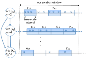
Figure 1: Scheme of the measurement scenario.

We assume that the network evolution is triggered by a universal slotted time, $t\in{\mathbb{Z}_{\geq 0}}$, not necessarily known by the monitors. The monitors communicate according to a time-dependent directed communication graph $t\mapsto G(t)=(\{1,\dots,N\},E(t))$, where $\{1,\dots,N\}$ are the monitor identifiers and the edge set $E(t)$ describes the communication among monitors: $(i,k)\in E(t)$ if monitor $i$ communicates to $k$ at time $t\in{\mathbb{Z}_{\geq 0}}$. For each node $i$, the nodes sending information to $i$ at time $t$, i.e., the set of $k\in\{1,\dots,N\}$ such that $(k,i)\in E(t)$ is the set of in-neighbors of $i$ at time $t$, and is denoted by $N^{I}_{i}(t)$. We make the following minimal assumption on the graph connectivity. First, we recall that a fixed directed graph is strongly connected if for any pair of nodes, $i$ and $j$, there exists a directed path (i.e., a set of consecutive edges) from $i$ to $j$.

Assumption II.1 (Uniform joint strong connectivity).

There exists an integer $Q\geq 1$ such that the graph $\left(\{1,\ldots,N\},\bigcup_{\tau=tQ}^{(t+1)Q-1}E(\tau)\right)$ is strongly connected $\forall\,t\geq 0$.

It is worth remarking that this network setup is very general, since it naturally embeds asynchronous scenarios as well as missing measurements due to, e.g., sensor failures.

III Distributed arrival rate estimation
via Empirical Bayes

In a decentralized set-up, in which nodes do not communicate, each node could estimate $\lambda_{i}$ based on the sample $\{y_{i,\ell}\}_{\ell=1,\ldots,n_{i}}$ by simply computing the empirical mean of the available measurements. That is, the decentralized estimator is

$$\hat{\lambda}^{\text{dec}}_{i}=\frac{1}{n_{i}}\sum_{\ell=1}^{n_{i}}y_{i,\ell}=\frac{\sigma_{i}}{n_{i}}$$

where $\sigma_{i}\stackrel{{\scriptstyle\textrm{\tiny def}}}{{=}}\sum_{\ell=1}^{n_{i}}y_{i,\ell}$.

Notice that, the decentralized estimator turns out to be the ML estimator of $\lambda_{i}$ when node $i$ can use only its own data. However, decentralized estimation yields reliable estimates only when the number of samples $n_{i}$ is large enough.

In our heterogenous set-up, it may happen that some nodes satisfy such a condition, while other ones do not have enough data, thus resulting in a poor estimation. In this paper we propose a distributed estimation scheme in which every node, especially the ones with fewer measurements, take advantage from cooperating with neighboring nodes.

How the measurements at other nodes can help the local estimation at a given node is a nontrivial issue and needs to be investigated by means of a suitable probabilistic framework. Specifically, we adopt a Bayesian model in which all the unknown arrival rates $\lambda_{i}$s are i.i.d. random variables ruled by a common probability distribution that captures the spatial variability of the process intensity.

This model belongs to the family of Poisson mixtures and is broadly accepted in the (centralized) statistical literature for modeling non-homogeneous scenarios, see, e.g., [22, 23], and [24, and references therein] for a through and extensive survey of properties and applications. As customary, see, e.g., [26], we adopt as common distribution the conjugate prior of the Poisson, which is the Gamma distribution. This choice allows one to obtain a close-form expression for the posterior (predictive) distribution. However, notice that, our model extends the classical Gamma-Poisson mixture since the sample sizes $n_{i}$, $i\in\{1,\dots,N\}$, can be different and thus exhibits even more flexibility.

A scheme of the proposed Bayesian framework for our network scenario is depicted in Figure 2.

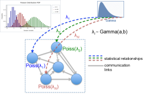
Figure 2: Scheme of the Bayesian model

III-A Empirical Bayes approach in monitoring networks

In applying a Bayesian estimation approach to a network context, the assumption that the prior distribution is fully known to all monitors is rather strong and may be a severe limitation in realistic scenarios. To overcome this limitation we adopt the Empirical Bayes approach in which only the class of the prior is known, i.e., $\lambda_{i}\sim\text{Gamma}(a,b)$, where the shape parameter $a$ is known, but the scale parameter $b$ is unknown. The assumption that $a$ is known, while only $b$ is unknown, says that only the shape of the Gamma distribution (determined by the parameter $a$) is known, while the scaling is not. This assumption is reasonable in many applications, since it is a way to embed a rough information on the phenomenon, and is customary for the sake of mathematical tractability, [26].

The hyperparameter $b$ can be estimated via a ML procedure. To this aim, we need the joint distribution of all measurements $\{y_{i,\ell}\}_{\ell=1,\ldots,n_{i}}$ for each agent $i$. The likelihood function is the product of the marginal distributions of all agents

$$L(\bm{y}_{1},\ldots,\bm{y}_{N}|b)=\prod_{i=1}^{N}p(\bm{y}_{i}|b)$$ (1)

where $\bm{y}_{i}=[y_{i,1}\ \cdots\ y_{i,n_{i}}]^{T}$. The marginal distribution of agent $i$ is derived from the joint distribution of $\bm{y}_{i}$ and $\lambda_{i}$,

$$p(\bm{y}_{i}|b) =\int_{0}^{\infty}\left(\prod_{\ell=1}^{n_{i}}f(y_{i,\ell}|\lambda_{i},b)\right)p(\lambda_{i}|b)\mathrm{d}\lambda_{i}$$

$$=\int_{0}^{\infty}\frac{\lambda_{i}^{\sigma_{i}}e^{-n_{i}\lambda_{i}}}{\prod_{\ell=1}^{n_{i}}y_{i,\ell}!}\frac{\lambda_{i}^{a-1}e^{-\lambda_{i}/b}}{\Gamma(a)b^{a}}\mathrm{d}\lambda_{i}$$

$$=\frac{\Gamma(\sigma_{i}+a)}{\Gamma(a)b^{a}\prod_{\ell=1}^{n_{i}}y_{i,\ell}!}\left(\frac{b}{n_{i}b+1}\right)^{\sigma_{i}+a}$$ (2)

By using eq. (2) into eq. (1) the likelihood is rewritten as:

$$L(\bm{y}_{1},\ldots,\bm{y}_{N}|b)\propto\frac{1}{b^{aN}}\prod_{i=1}^{N}\left(\frac{b}{n_{i}b+1}\right)^{\sigma_{i}+a}.$$ (3)

Thus, the ML estimator $\hat{b}^{\text{ML}}$ of $b$ can be found by solving the following optimization problem

$$\hat{b}^{\text{ML}} =\operatorname*{arg\,min}_{b\in\mathbb{R}_{+}}\!\left\{\!aN\log b-\!\sum_{i=1}^{N}(\sigma_{i}+a)\log\!\left(\frac{b}{n_{i}b+1}\right)\right\}\!\!$$

$$=\operatorname*{arg\,min}_{b\in\mathbb{R}_{+}}\sum_{i=1}^{N}f(b;n_{i},\sigma_{i}).$$ (4)

The problem can be solved in closed-form only for the homogeneous case where all $n_{i}$s are equal, i.e., for $n_{i}=n/N$, recalling that $n$ is the total number of measurements. In this case the ML estimator of $b$ based on the entire set of measurements is given by

$$\hat{b}^{\text{hom}}=\frac{1}{an}\sum_{i=1}^{N}\sigma_{i}=\frac{\sigma}{an}$$

where $n\stackrel{{\scriptstyle\textrm{\tiny def}}}{{=}}\sum_{i=1}^{N}n_{i}$, and $\sigma\stackrel{{\scriptstyle\textrm{\tiny def}}}{{=}}\sum_{i=1}^{N}\sigma_{i}$.

After obtaining an estimate for $b$, the Empirical Bayes estimator of the arrival rate $\lambda_{i}$ that minimizes the Mean Square Error (MMSE) can be obtained by computing the conditional mean of the posterior distribution $p(\lambda_{i}|\bm{y}_{i},b)$. The latter is given by the ratio between the joint pdf $p(\bm{y}_{i},\lambda_{i}|b)$ and the marginal pdf $p(\bm{y}_{i}|b)$ as from eq. (2), i.e.,

$$p(\lambda_{i}|\bm{y}_{i},b)=\frac{\lambda_{i}^{\sigma_{i}+a-1}e^{-\lambda_{i}\frac{n_{i}b+1}{b}}}{\Gamma(\sigma_{i}+a)}\left(\frac{b}{n_{i}b+1}\right)^{-\sigma_{i}-a}$$ (5)

Eq. (5) is a Gamma pdf with parameters $(\sigma_{i}+a,\frac{b}{n_{i}b+1})$, hence the Empirical Bayes MMSE estimator of each $\lambda_{i}$ is

$$\hat{\lambda}^{\text{EB}}_{i}=\mathrm{E}[\lambda_{i}|\bm{y}_{i},\hat{b}^{\text{ML}}]=\frac{\hat{b}^{\text{ML}}}{\hat{b}^{\text{ML}}n_{i}+1}(a+\sigma_{i}).$$ (6)

Remark III.1.

It is worth highlighting that the Bayesian estimate is especially useful when $n_{i}$ is small. In fact, nodes improve the quality of their local estimate by combining the frequentist estimation (based only on local observations) with a correction term (based on a prior global knowledge), which is estimated in a cooperative way. Indeed, we can rewrite $\hat{\lambda}^{\text{EB}}_{i}=\rho\frac{\sigma_{i}}{n_{i}}+(1-\rho)a\hat{b}^{\text{ML}}$, with $\rho=\frac{\hat{b}^{\text{ML}}n_{i}}{\hat{b}^{\text{ML}}n_{i}+1}$. When the local information is abundant ($n_{i}\rightarrow\infty$ and thus $\rho\rightarrow 1$), the MMSE estimator (6) tends towards $\hat{\lambda}^{\text{dec}}_{i}$, meaning that when $n_{i}$ is large no further information can be inferred from the network. Conversely, when local information is scarce, i.e., the sample size $n_{i}$ is small, even one, the MMSE estimator (6) approaches the estimate of the global mean $\mathrm{E}[\lambda_{i}]=ab$.

In the following we will also consider an ad-hoc estimator obtained by using $\hat{b}^{\text{hom}}$ instead of the optimal $\hat{b}^{\text{ML}}$, i.e.,

$$\hat{\lambda}^{\text{ad-hoc}}_{i}\stackrel{{\scriptstyle\textrm{\tiny def}}}{{=}}\frac{\hat{b}^{\text{hom}}}{\hat{b}^{\text{hom}}\,n_{i}+1}(a+\sigma_{i})=\frac{\sigma}{an+\sigma n_{i}}(a+\sigma_{i}).$$

Clearly, the estimator $\hat{\lambda}^{\text{EB}}_{i}$ follows the “rationale” of the Empirical Bayes approach and, therefore, has performance guarantees inherited from the ML procedure. Conversely, the ad-hoc estimator is an alternative that at the moment has the only advantage of having a closed-form expression, whose performances need to be understood. In the rest of the paper we will show that, not only this estimator leads to a simpler and faster distributed algorithm, but also that for large number of agents performs as $\hat{\lambda}^{\text{EB}}_{i}$.

III-B Distributed estimators

From eq. (6) it is clear that each agent can compute the Empirical Bayes MMSE estimator provided it knows $\hat{b}^{\text{ML}}$. Optimization problem (III-A), giving the ML estimator of $b$, has a separable cost (i.e., the sum of $N$ local costs), hence it can be solved by using available distributed optimization algorithms for asynchronous networks [27, 13]. We propose a distributed estimator in which each node implements the local update rule of the chosen distributed optimization algorithm.

The ML estimation problem (III-A) is not guaranteed to be convex in general. This is quite common in the estimation literature. However, since the function is coercive, there exists (at least) a minimizer and, thus, it is reasonable to apply descent algorithms, as the one in [13], which, under suitable conditions, guarantee convergence to a local minimizer.

The Empirical Bayes distributed estimator  is as follows. At each $t\in{\mathbb{Z}_{\geq 0}}$, each agent $i$ stores a local state $\xi_{i}(t)$, an estimate $\hat{b}^{\text{ML}}_{i}(t)$ of $\hat{b}^{\text{ML}}$ and an estimate $\hat{\lambda}^{\text{EB}}_{i}(t)$ of $\hat{\lambda}^{\text{EB}}_{i}$. The node initializes its local state $\xi_{i}$ to an initial value $\xi_{i0}$ chosen according to the distributed optimization algorithm in use, and sets $\hat{b}^{\text{ML}}_{i}(0)=\sigma_{i}/(an_{i})$ (which would be the solution of (III-A) if $i$ were the only agent). Then it updates its estimate of $\hat{b}^{\text{ML}}$ by using the local update rule of the chosen distributed optimization algorithm, and updates the current estimate $\hat{\lambda}^{\text{EB}}_{i}(t)$ by using (6). The algorithm is defined formally in the following table. For each $t\in{\mathbb{Z}_{\geq 0}}$, let $\{\hat{\xi}_{k}(t)\}_{k\in N^{I}_{i}(t)}$ be the collection of states of the in-neighbors of node $i$, opt_local the local update of the chosen distributed optimization algorithm, and $\gamma(t)$ an algorithm parameter as, e.g., a time-varying step-size.

Algorithm 1 Empirical Bayes distributed estimator

  Initialization: $\xi_{i}(0)=\xi_{i0}$, $\hat{b}^{\text{ML}}_{i}(0)=\frac{\sigma_{i}}{an_{i}}$.

  Iterate:

$$(\hat{b}^{\text{ML}}_{i} (t+1),\hat{\xi}_{i}(t+1))=$$

$$\texttt{opt\_local}\left(\hat{b}^{\text{ML}}_{i}(t),\hat{\xi}_{i}(t),\{\hat{\xi}_{k}(t)\}_{k\in N^{I}_{i}(t)};\gamma(t)\right)\!,$$

$$\hat{\lambda}^{\text{EB}}_{i} (t+1)=\frac{\hat{b}^{\text{ML}}_{i}(t+1)}{\hat{b}^{\text{ML}}_{i}(t+1)n_{i}+1}(a+\sigma_{i}).$$

As an example, we show the opt_local function for the distributed subgradient-push method proposed in [13]. To be consistent with the notation in [13] we let $\xi_{i}=(v_{i},y_{i},x_{i})$, which is initialized to $(v_{i}(0),y_{i}(0),x_{i}(0))=(1,1,x_{i0})$, with $x_{i0}$ an arbitrary initial value. Also, $d_{k}(t)$ denotes the number of out-neighbors of node $k$ at time $t$.

function $\xi_{i}(t+1)=\\ \phantom{aaa}\texttt{opt\_local}\left(\hat{b}^{\text{ML}}_{i}(t),\hat{\xi}_{i}(t),\{\hat{\xi}_{k}(t)\}_{k\in N^{I}_{i}(t)};\gamma(t)\right)\!$

$$v_{i}(t+1) =\sum_{k\in N_{i}^{I}(t)\cup\{i\}}\frac{x_{k}(t)}{d_{k}(t)}$$

$$y_{i}(t+1) =\sum_{k\in N_{i}^{I}(t)\cup\{i\}}\frac{y_{k}(t)}{d_{k}(t)}$$

$$\hat{b}^{\text{ML}}_{i}(t+1) =\frac{v_{i}(t+1)}{y_{i}(t+1)}$$

$$x_{i}(t+1) =v_{i}(t+1)-\gamma(t+1)\nabla f(\hat{b}^{\text{ML}}_{i}(t+1);n_{i},\sigma_{i})$$

with $\nabla f(b;n_{i},\sigma_{i})=\frac{a}{b(n_{i}b+1)}(an_{i}b-\sigma_{i})$.

If problem (III-A) has a unique minimizer, the distributed optimization algorithm guarantees that all nodes reach consensus on the global minimizer. That is,

$$\lim_{t\rightarrow\infty}\hat{b}^{\text{ML}}_{i}(t)=\hat{b}^{\text{ML}},\qquad\text{for all $i\in\{1,\dots,N\}$}.$$

From the convergence properties of the chosen distributed optimization algorithm it follows immediately that the proposed distributed estimator asymptotically computes at each node $i$ the Empirical Bayes MMSE estimator of $\lambda_{i}$.

However, most of the available distributed optimization algorithms, as the ones in [27, 13], need the tuning of a global parameter (we denoted it $\gamma$), and typically exhibit a sub-exponential convergence even in static graphs. To overcome these drawbacks, we propose an alternative distributed estimator with reduced complexity that, although suboptimal, will be shown to perform comparably to the optimal one.

The ad-hoc distributed estimator  is defined as follows. For each $t\in{\mathbb{Z}_{\geq 0}}$, each node $i\in\{1,\dots,N\}$ stores in memory two local states $s_{i}(t)$ and $\eta_{i}(t)$, an estimate $\hat{b}^{\text{hom}}_{i}(t)$ of $\hat{b}^{\text{hom}}$, and an estimate $\hat{\lambda}^{\text{ad-hoc}}_{i}(t)$ of $\hat{\lambda}^{\text{ad-hoc}}_{i}$. Let $w_{ik}(t)\in{\mathbb{R}}_{\geq 0}$ be a set of weights such that $w_{ik}(t)>0$ if $(i,k)\in E(t)$ or $k=i$, and $w_{ik}(t)=0$ otherwise. The ad-hoc distributed estimator is given in the following table.

Algorithm 2 ad-hoc distributed estimator

  Initialization: $s_{i}(0)=\sigma_{i}$, $\eta_{i}(0)=n_{i}$, $\hat{b}^{\text{hom}}_{i}(0)=\sigma_{i}/(an_{i})$, $\hat{\lambda}^{\text{ad-hoc}}_{i}(0)=\frac{\hat{b}^{\text{hom}}_{i}(0)}{\hat{b}^{\text{hom}}_{i}(0)n_{i}+1}(a+\sigma_{i})$.

  Iterate:

$$s_{i}(t+1) =\sum_{k\in N_{i}^{I}(t)\cup\{i\}}w_{ik}(t)s_{k}(t)$$

$$\eta_{i}(t+1) =\sum_{k\in N_{i}^{I}(t)\cup\{i\}}w_{ik}(t)\eta_{k}(t)$$

$$\hat{b}^{\text{hom}}_{i}(t+1) =\frac{1}{a}\,\frac{s_{i}(t+1)}{\eta_{i}(t+1)}$$

$$\hat{\lambda}^{\text{ad-hoc}}_{i}(t+1) =\frac{\hat{b}^{\text{hom}}_{i}(t+1)}{\hat{b}^{\text{hom}}_{i}(t+1)n_{i}+1}(a+\sigma_{i}).$$

We can rewrite the update of $\eta_{i}(t)$ and $s_{i}(t)$ by using an aggregate dynamics. That is, let $\eta(t)=[\eta_{1}(t)\ldots\eta_{N}(t)]^{T}$ and $s(t)=[s_{1}(t)\ldots s_{N}(t)]^{T}$ be the aggregate states, their dynamics is given by

$$\begin{split}s(t+1)&=W(t)s(t)\\ \eta(t+1)&=W(t)\eta(t)\end{split}$$ (7)

with $s(0)=[\sigma_{1}\ldots\sigma_{N}]^{T}\stackrel{{\scriptstyle\textrm{\tiny def}}}{{=}}\bm{\sigma}$, $\eta(0)=[n_{1}\ldots n_{N}]^{T}\stackrel{{\scriptstyle\textrm{\tiny def}}}{{=}}\bm{n}$ and $W(t)$ the matrix with elements $w_{ij}(t)$. Let us denote

$$\Phi(t)=W(t-1)\cdots W(0)$$ (8)

the state transition matrix associated to each one of the linear systems (7), so that

$$\begin{split}s(t)&=\Phi(t)s(0)\\ \eta(t)&=\Phi(t)\eta(0).\end{split}$$ (9)

For the algorithm to converge we need the following assumption together with the Assumption II.1 (uniform joint connectivity of the communication digraph).

Assumption III.2 (Properties of $W(t)$).

For each $t\in{\mathbb{Z}_{\geq 0}}$, the matrix $W(t)$ is column stochastic, i.e., $\sum_{i=1}^{n}w_{ik}(t)=1$, and there exists a positive constant $\alpha>0$ such that $w_{ii}(t)>\alpha$ and $w_{ik}(t)\in\{0\}\cup[\alpha,1]$.

Remark III.3.

It is worth noting that the column stochasticity assumption above is not the usual assumption used in linear consensus algorithms in which row stochasticity is assumed.

Lemma III.4.

Let $t\mapsto G(t)$ be a uniformly jointly strongly connected graph (Assumption II.1) and $\{W(t)\}_{t\geq 0}$ a sequence of matrices satisfying Assumption III.2. Then denoting $\Phi(t)=W(t)W(t-1)\cdots W(0)$ with $(i,k)$ element $\phi_{ik}(t)$, the following holds true.

1. The matrix sequence $\{W(t)\}_{t\geq 0}$ is weakly ergodic, i.e.,

   $$\lim_{t\rightarrow\infty}|\phi_{ik}(t)-\phi_{ih}(t)|=0$$

   for all $i,k,h\in\{1,\dots,N\}$.

2. There exists some $\mu>0$ such that for all $t\geq 0$, $\textbf{1}^{T}\Phi(t)\geq\mu>0$, i.e., for any $i\in\{1,\dots,N\}$,

   $$\sum_{k=1}^{N}\phi_{ik}(t)>\mu.$$

The result is well-known and can be found, e.g., in [13]. Further references on this result under the same or different connectivity assumptions are [28, 29, 30, 31].

Proposition III.5.

Let Assumption II.1 hold. Then the ad-hoc distributed estimator  (Algorithm 2) satisfies

$$\begin{split}\lim_{t\rightarrow\infty}\hat{b}^{\text{hom}}_{i}(t)&=\hat{b}^{\text{hom}}\\ \lim_{t\rightarrow\infty}\hat{\lambda}^{\text{ad-hoc}}_{i}(t)&=\hat{\lambda}^{\text{ad-hoc}}_{i}.\end{split}$$

Proof.

From Lemma III.4, $\{W(t)\}_{t\geq 0}$ is weakly ergodic so that there exists a sequence of stochastic vectors $\bar{\phi}(t)=[\bar{\phi}_{1}(t)\ldots\bar{\phi}_{N}(t)]$ such that for each $i\in\{1,\dots,N\}$, $\phi_{ik}(t)\rightarrow\bar{\phi}_{i}(t)$ for all $k\in\{1,\dots,N\}$. From eq. (9) it follows that

$$s_{i}(t)\rightarrow\bar{\phi}_{i}(t)\sum_{k=1}^{N}s_{k}(0)=\bar{\phi}_{i}(t)\sum_{k=1}^{N}\sigma_{k}(0)$$

and

$$\eta_{i}(t)\rightarrow\bar{\phi}_{i}(t)\sum_{k=1}^{N}\eta_{k}(0)=\bar{\phi}_{i}(t)\sum_{k=1}^{N}n_{k}(0).$$

Thus, $\frac{s_{i}(t)}{\eta_{i}(t)}\rightarrow\frac{\sum_{k=1}^{N}\sigma_{k}(0)}{\sum_{k=1}^{N}n_{k}(0)}$, so that the proof follows. ∎

Remark III.6 (Connectivity assumption).

The result of Proposition III.5 can be proven also if Assumption II.1 is replaced by Assumption 1 in [31], that is if $\{W(t)\}_{t\geq 0}>0$ is a stationary and ergodic sequence of stochastic matrices with positive diagonals, and $\mathrm{E}[W]$ is irreducible. The result can be proven by following the same line of proof developed therein. Thus, the ad-hoc estimator could be implemented also in a monitoring network with stochastic gossip communication.

Remark III.7.

The proposed algorithms are based on the assumption that the arrival-rates are constant in the observation window. Therefore, one can apply the algorithms iteratively by recomputing the estimates on different windows of data, thus getting time-varying arrival-rates.

To conclude this section, we point out that the update of the subgradient push optimization algorithm includes a push-sum consensus step, i.e., a diffusive update based on a column stochastic matrix (with coefficients $w_{ik}(t)=1/d_{k}(t)$ for $k\in N_{i}(t)$), which is the same used in the ad-hoc distributed estimator  (Algorithm 2). However, in the subgradient push this update is part of a gradient descent step. In fact, the role and the evolution of the involved variables, i.e., $(s_{i},\eta_{i})$ and $(v_{i},y_{i})$ respectively, are different as well as the convergence rates. Indeed, the ad-hoc estimator exhibits the exponential convergence of linear consensus protocols as opposed to the much slower $O(\ln t/\sqrt{t})$ rate of the subgradient-push [13].

These considerations, together with the lower computational burden, make the ad-hoc distributed estimator  appealing even though not optimal. In the following section we will show that it actually performs very closely to the MMSE estimator.

IV Estimator performance analysis

In this section we analyze the performance of the proposed distributed estimators. In particular, for the Empirical Bayes distributed estimator, lacking a closed form for the update rule of $\hat{b}^{\text{ML}}$ and, in turn, of $\hat{\lambda}^{\text{EB}}$, we are able to derive only steady-state ($t\rightarrow\infty$) and asymptotic ($N\rightarrow\infty$) bounds. Conversely, for the ad-hoc distributed estimator  a transient analysis (at any $t\in{\mathbb{Z}_{\geq 0}}$) can be derived for any $N\in{\mathbb{N}}$.

To develop the performance analysis, we consider a “special” agent, we label it as $j$, that does not participate to the computation of $\hat{b}^{\text{ML}}$ (respectively $\hat{b}^{\text{hom}}$). Under this assumption, it turns out that $\sigma_{j}$ is independent of $\hat{b}^{\text{ML}}$ (respectively $\hat{b}^{\text{hom}}$). Clearly, $\sigma_{j}$ is also independent of any local estimate $\hat{b}^{\text{ML}}_{i}(t)$ (respectively $\hat{b}^{\text{hom}}_{i}(t)$), $i\in\{1,\dots,N\}$, at any $t\in{\mathbb{Z}_{\geq 0}}$. Consistently, here we can simply assume that for the computation of $\hat{\lambda}^{\text{EB}}_{j}(t)$ (respectively $\hat{\lambda}^{\text{ad-hoc}}_{j}(t)$), agent $j$ uses the local estimate of $b$ computed by one of its in-neighbors, that is, e.g., $\hat{b}^{\text{hom}}_{j}(t)=\hat{b}^{\text{hom}}_{i}(t)$ for some $i\in N_{j}^{I}(t)\subset\{1,\dots,N\}$.

Notice that, in practice, the analysis developed for such an agent $j$ holds approximately for any node in the network participating to the distributed computation. Indeed, due to the large number of agents $N$, for any agent $i$ (running the distributed algorithm), $\hat{b}^{\text{ML}}$ (respectively $\hat{b}^{\text{hom}}$) and $\sigma_{i}$ are very weakly correlated. The validity of this statement will be corroborated by the Monte Carlo analysis in the next section.

We start by deriving the Cramer-Rao lower bound (CRB) for any unbiased estimator $\hat{b}$ of $b$, i.e.,

$$\mathrm{VAR}[\hat{b}]\geq\mathrm{CRB}(b).$$

Lemma IV.1.

The CRB for the estimation of the hyperparameter $b$ is given by

$$\mathrm{CRB}(b)=\frac{b/a}{\sum_{i=1}^{N}\frac{n_{i}}{n_{i}b+1}}.$$ (10)

The proof is reported in Appendix -A.

IV-A Analysis of the Empirical Bayes distributed estimator

For the Empirical Bayes distributed estimator  we can analyze the performance only once consensus on the optimal value $\hat{b}^{\text{ML}}$, and thus on $\hat{\lambda}^{\text{EB}}_{j}$, has been reached. Specifically, let us recall that

$$\hat{\lambda}^{\text{EB}}_{j}=\frac{\hat{b}^{\text{ML}}}{\hat{b}^{\text{ML}}n_{j}+1}(a+\sigma_{j}).$$ (11)

Despite no analytical expression is available for the ML estimator $\hat{b}^{\text{ML}}$ (nor for its moments) the asymptotic analysis ($N\rightarrow\infty$) of the corresponding MMSE estimator $\hat{\lambda}^{\text{EB}}_{j}$ can be obtained by using the properties of ML estimation. In particular, any ML estimator is asymptotically unbiased and efficient, hence $\mathrm{E}[\hat{b}^{\text{ML}}]\rightarrow b$ and $\mathrm{VAR}[\hat{b}^{\text{ML}}]\rightarrow\mathrm{CRB}(b)$ as $N\rightarrow\infty$. From equation (10),

$$\mathrm{CRB}(b) =\frac{b/a}{\sum_{i=1}^{N}\frac{n_{i}}{n_{i}b+1}}$$

$$\leq\frac{b/a}{\sum_{i=1}^{N}\frac{1}{n_{\text{max}}b+1}}=\frac{b/a}{N\frac{1}{n_{\text{max}}b+1}}\stackrel{{\scriptstyle N\rightarrow\infty}}{{\xrightarrow{\hskip 28.45274pt}}}0\,,$$ (12)

so that $\mathrm{VAR}[\hat{b}^{\text{ML}}]\rightarrow 0$ as $N\rightarrow\infty$.

These results on the asymptotic properties of $\hat{b}^{\text{ML}}$ can be used to prove the following theorem characterizing the asymptotic behavior of the Empirical Bayes distributed estimator .

Due to the nonlinear dependency of $\hat{\lambda}^{\text{EB}}$ from $\hat{b}^{\text{ML}}$, we will perform an approximate analysis by considering the Taylor expansion of $\hat{\lambda}^{\text{EB}}$ around $\mathrm{E}[\hat{b}^{\text{ML}}]$. For tractability we will consider respectively the second-order and the first-order approximations for mean and variance. The numerical analysis in Section V will confirm the validity of such an approximation.

Theorem IV.2.

Consider a network of monitors as in Section II running the Empirical Bayes distributed estimator. Then, as $N\rightarrow\infty$, it holds true

$$\mathrm{E}[\hat{\lambda}^{\text{EB}}_{j}|\lambda_{j}]\longrightarrow\frac{b}{1+n_{j}b}(a+n_{j}\lambda_{j}).$$ (13)

to second order and

$$\mathrm{VAR}[\hat{\lambda}^{\text{EB}}_{j}|\lambda_{j}]\longrightarrow\left(\frac{b}{1+n_{j}b}\right)^{2}n_{j}\lambda_{j},$$ (14)

to first order.

IV-B Analysis of the ad-hoc distributed estimator

The closed-form update of the ad-hoc distributed estimator  allows us to perform a more detailed analysis. In particular, we are able to characterize mean and variance of the local estimator $\hat{\lambda}^{\text{ad-hoc}}_{j}(t)$ during the algorithm evolution (transient analysis) and for any fixed value of the number of nodes $N$.

As we have done for the Empirical Bayes distributed estimator, also for the ad-hoc one we first characterize the estimator of the hyperparameter $b$.

Before addressing the transient analysis, we compute mean and variance of the consensus value $\hat{b}^{\text{hom}}$.

Proposition IV.3.

The homogeneous estimator of $b$, $\hat{b}^{\text{hom}}$, is unbiased, i.e.,

$$\mathrm{E}[\hat{b}^{\text{hom}}]=b,$$

and has variance

$$\mathrm{VAR}[\hat{b}^{\text{hom}}]=\frac{b}{an}+\frac{b^{2}}{an^{2}}\sum_{i=1}^{N}n_{i}^{2}\,.$$ (15)

Moreover, the estimator $\hat{b}^{\text{hom}}$ is consistent, i.e., it converges in probability to the true value $b$ as $N\rightarrow\infty$.

The proof is given in Appendix -C.

Remark IV.4.

The estimator $\hat{b}^{\text{hom}}$ is the ML estimator in the homogenous case, i.e., when $n_{i}=n/N$ for all $i\in\{1,\dots,N\}$, and it attains the Cramer-Rao Bound (CRB) not only asymptotically, but for any $N$. It follows by substituting $n_{i}=n/N$ in (10) and (15). Interestingly, we will show in the numerical analysis that even in the non-homogeneous scenario the ML estimator $\hat{b}^{\text{ML}}$ approaches the CRB at any fixed $N$.

The following lemma gives a characterization of the transient local estimates.

Lemma IV.5.

Let Assumption II.1 and Assumption III.2 hold. For all $i\in\{1,\dots,N\}$, the local estimator $\hat{b}^{\text{hom}}_{i}(t)$ used in the ad-hoc distributed estimator  (Algorithm 2) is unbiased at any $t\in{\mathbb{Z}_{\geq 0}}$, i.e.,

$$\mathrm{E}[\hat{b}^{\text{hom}}_{i}(t)]=b,$$

and has variance

$$\begin{split}\mathrm{VAR}[\hat{b}^{\text{hom}}_{i}(t)]=\frac{b}{a}\frac{\sum_{k=1}^{N}\phi_{ik}(t)^{2}n_{k}}{{\left(\sum_{k=1}^{N}\phi_{ik}(t)n_{k}\right)^{2}}}+\frac{b^{2}}{a}\frac{\sum_{k=1}^{N}\phi_{ik}(t)^{2}n_{k}^{2}}{\left(\sum_{k=1}^{N}\phi_{ik}(t)n_{k}\right)^{2}}\end{split}$$ (16)

where $\phi_{ik}(t)$ is the element $(i,k)$ of the state transition matrix $\Phi(t)$ defined in (8).

Moreover, as $t\rightarrow\infty$, the variance of $\hat{b}^{\text{hom}}_{i}(t)$ converges exponentially to the variance of $\hat{b}^{\text{hom}}$, (15), and satisfies

$$|\mathrm{VAR}[\hat{b}^{\text{hom}}_{i}(t)]-\mathrm{VAR}[\hat{b}^{\text{hom}}]|\leq\frac{b(1+2bn_{\text{max}})}{\mu a}\delta(\Phi(t)),$$ (17)

where $\mu>0$ is given in Lemma III.4 and $\delta(\Phi(t))$ is a (proper) coefficient of ergodicity (exponentially decaying with time) defined as $\displaystyle\delta(A)\stackrel{{\scriptstyle\textrm{\tiny def}}}{{=}}\max_{k}\max_{i_{1},i_{1}}|a_{i_{1},k}-a_{i_{2},k}|$.

The proof is reported in Appendix -D.

Remark IV.6.

It is worth noting that $\mu$ and $\delta(\Phi(t))$ in equation (17) typically depend on $N$ (and thus also on $n$). The interesting aspect of the given result is that the bound provided in the previous lemma relates the convergence rate of $\mathrm{VAR}[\hat{b}^{\text{hom}}]$ to parameters of the communication graph and the diffusion protocol as $\mu$ and $\delta(\Phi(t))$. For example, if $\cup_{\tau=tQ}^{(t+1)Q-1}G(\tau)$ is balanced, the matrix $\Phi(t)$ is doubly stochastic, hence $\mu=1$.

With this characterization of the hyperparameter estimator, we are ready to analyze the estimator $\hat{\lambda}^{\text{ad-hoc}}_{j}(t)$. Recalling the assumption that the measurements of agent $j$ do not contribute to the computation of $\hat{b}^{\text{hom}}_{j}(t)$, we clearly have

$$\mathrm{E}[\hat{b}^{\text{hom}}_{j}(t)|\lambda_{j}]=\mathrm{E}[\hat{b}^{\text{hom}}_{j}(t)]=b.$$ (18)

and

$$\mathrm{VAR}[\hat{b}^{\text{hom}}_{j}(t)|\lambda_{j}]=\mathrm{VAR}[\hat{b}^{\text{hom}}_{j}(t)].$$

Remark IV.7.

It is worth noticing once more that although for a tractable, rigorous analysis we need the assumption that agent $j$ does not contribute to the distributed computation, in practice the results hold with good approximation also in the scenario in which agent $j$ contributes to the distributed computation. This is due to the weak impact of single measurements onto the aggregate quantities. In fact, for example, following analogous calculations as in the proof of Lemma IV.5, the conditional mean in this latter case turns out to be

$$\mathrm{E}[\hat{b}^{\text{hom}}_{j}(t)|\lambda_{j}]=b-\frac{\phi_{jj}(t)n_{j}}{\eta_{j}(t)}\left(b-\frac{\lambda_{j}}{a}\right),$$ (19)

where $\phi_{jj}(t)$ is, again, the element $(j,j)$ of $\Phi(t)$ and we have also used that, conditioned to the $\lambda_{j}$ of agent $j$,

$$\mathrm{E}[y_{i,\ell}|\lambda_{j}]=\left\{\begin{array}[]{ll}\lambda_{j}&i=j\\ ab&i\neq j\end{array}\right..$$

Since as $t\rightarrow\infty$, $\frac{\phi_{jj}(t)n_{j}}{\eta_{j}(t)}\rightarrow\frac{n_{j}}{n}\ll 1$, then the difference between equations (19) and (18) is practically negligible.

In the next theorem we provide explicit transient expressions for the conditional mean and variance of $\hat{\lambda}^{\text{ad-hoc}}_{j}(t)$. Again, we use second-order and first-order approximations respectively.

Theorem IV.8.

Consider a network of monitors as in Section II running the ad-hoc distributed estimator  (Algorithm 2). Then the transient conditional mean and variance of $\hat{\lambda}^{\text{ad-hoc}}_{j}(t)$ are given by

$$\;\;\;\mathrm{E}[ \hat{\lambda}^{\text{ad-hoc}}_{j}(t)|\lambda_{j}]\approx$$

$$(a+n_{j}\lambda_{j})\left[\frac{b}{1+n_{j}b}-\frac{n_{j}}{(1+n_{j}b)^{3}}\mathrm{VAR}[\hat{b}^{\text{hom}}_{j}(t)]\right]$$ (20)

and

$$\mathrm{VAR}[ \hat{\lambda}^{\text{ad-hoc}}_{j}(t)|\lambda_{j}]\approx$$

$$\left[\frac{b}{1+n_{j}b}-\!\frac{n_{j}}{(1+n_{j}b)^{3}}\mathrm{VAR}[\hat{b}^{\text{hom}}_{j}(t)]\right]^{2}n_{j}\lambda_{j}$$

$$\;\;+\left[\frac{2n_{j}}{(1+n_{j}b)^{3}}\right]^{2}\mathrm{VAR}[\hat{b}^{\text{hom}}_{j}(t)]\left[(a+n_{j}\lambda_{j})^{2}+n_{j}\lambda_{j}\right]$$ (21)

where $\approx$ indicates respectively the second-order and the first-order approximations, and $\mathrm{VAR}[\hat{b}^{\text{hom}}_{j}(t)]$ is given in (16).

Moreover, the asymptotic value $\hat{\lambda}^{\text{ad-hoc}}_{j}$ satisfies, as $N\rightarrow\infty$,

$$\mathrm{E}[\hat{\lambda}^{\text{ad-hoc}}_{j}|\lambda_{j}] \longrightarrow\frac{b}{1+n_{j}b}(a+n_{j}\lambda_{j})$$ (22)

to second order and

$$\mathrm{VAR}[\hat{\lambda}^{\text{ad-hoc}}_{j}|\lambda_{j}] \longrightarrow\left(\frac{b}{1+n_{j}b}\right)^{2}n_{j}\lambda_{j}$$ (23)

to first order.

Remark IV.9.

By comparing equations (22)-(23) with (13)-(14), one can notice that at steady-state ($t\rightarrow\infty$) and for large number of agents ($N\rightarrow\infty$) the mean and variance of the ad-hoc distributed estimator  approach the ones of the optimal Empirical Bayes. Moreover, the right-hand side of (23) can be rewritten as $\frac{\lambda_{j}}{n_{j}}\left(\frac{n_{j}b}{1+n_{j}b}\right)^{2}$, which is clearly smaller than the variance of the decentralized estimator $\mathrm{VAR}[\hat{\lambda}^{\text{dec}}_{j}|\lambda_{j}]=\frac{\lambda_{j}}{n_{j}}$.

V Numerical performance analysis

In this section we analyze the performance of the proposed estimators. Starting from the theoretical characterization developed in the previous section, we perform a Monte Carlo analysis confirming the theoretical bounds and adding other insights on the performance of the estimators.

As performance metric we adopt the Root Mean Square Error (RMSE), thus taking into account both bias and variance of the estimators. We recall that for an estimator $\hat{\omega}$ of a parameter $\omega$, the RMSE is defined as

$$\mathrm{RMSE}[\hat{\omega}] =\sqrt{\mathrm{E}[(\hat{\omega}-\omega)^{2}]}$$

$$=\sqrt{\mathrm{VAR}[\hat{\omega}]+\mathrm{E}^{2}[\hat{\omega}]-2\omega\mathrm{E}[\hat{\omega}]+\omega^{2}}.$$ (24)

Clearly, if the estimator is unbiased the RMSE coincides with the standard deviation, i.e., $\mathrm{RMSE}[\hat{\omega}]=\sqrt{\mathrm{VAR}[\hat{\omega}]}$.

The statistical RMSE, $\mathrm{RMSE}[\omega]$, will be compared with the sample value obtained through the Monte Carlo trials, $\mathrm{RMSE}_{MC}$, computed as

$$\mathrm{RMSE}_{MC}=\sqrt{\frac{1}{M}\sum_{m=1}^{M}(\hat{\omega}[m]-\omega)^{2}},$$

where $M$ is the number of trials and $\hat{\omega}[m]$ is the $m$th estimate of $\omega$.

In the following we set $M=5\times 10^{4}$ and, to generate the random values, we use a Gamma distribution with parameters $a=10$ and $b=1$, which gives values of $\lambda_{i}$ in the range $[1,25]$ with $99.98\%$ probability.

In order to challenge the ad-hoc distributed estimator we focus on a strongly inhomogeneous network scenario. That is, we consider a network in which half of the nodes have the maximum number of measurements in the observation window, $n_{i}=n_{\text{max}}$ (we set $n_{\text{max}}=50$), and the remaining ones only one measurement, $n_{i}=1$.

We start by analyzing the transient performance of the ad-hoc distributed estimator. Consistently with the theoretical analysis, we first focus on the time evolution of the RMSE of $\hat{b}^{\text{hom}}_{i}(t)$. Notice that, since $\hat{b}^{\text{hom}}_{i}(t)$ is an unbiased estimator it holds $\mathrm{RMSE}[\hat{b}^{\text{hom}}_{i}(t)]=\sqrt{\mathrm{VAR}[\hat{b}^{\text{hom}}_{i}(t)]}$. We compare the evolution of the sample RMSE with the theoretical expression obtained from (16). For this analysis we set $N=20$ and consider two possible communication models. In the first one we consider a fixed, directed and very sparse communication graph defined as follows: starting from a directed cycle, we add the edges $(3,1)$, $(3,2)$, $(4,1)$ and $(4,2)$ to unbalance the graph. In Figure 3 we plot the evolution of $\mathrm{RMSE}[\hat{b}^{\text{hom}}_{i}(t)]$ for $4$ nodes, two of them with $n_{\text{max}}$ measurements and two with one measurement. The theoretical curve predicts very accurately the sample RMSE obtained by the Monte Carlo trials, as highlighted in the inset. As expected, the RMSE of the different nodes converges to the consensus value $\mathrm{RMSE}[\hat{b}^{\text{hom}}]$ obtained from (15).

As a second scenario we challenge the algorithm on a time-varying topology. Namely, we consider a graph obtained by extracting at each time-instant an Erdős-Rényi graph with parameter $0.01$. We choose a small value, so that at a given instant the graph is disconnected with high probability, but it turns out to be uniformly jointly connected with $Q=36$.

In Figure 4 we again compare the theoretical evolutions of $\mathrm{RMSE}[\hat{b}^{\text{hom}}_{i}(t)]$ with their sample counterparts. We can highlight two main differences with respect to the previous scenario. The curves have some constant portions showing that nodes can be isolated for some time-intervals. However, the convergence is faster compared to the fixed scenario. This can be explained by the higher density of the union graph in the time-varying scenario as opposed to the sparsity of the fixed graph. In fact, we noticed that increasing the Erdős-Rényi graph parameter increases the convergence speed.

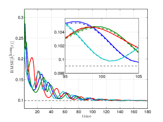
Figure 3: Time evolution of $\mathrm{RMSE}[\hat{b}^{\text{hom}}_{i}(t)]$ under fixed communication graph. The solid lines indicate the theoretical expressions, while the dash-dot lines are the ones obtained via Monte Carlo simulations. The dashed horizontal line is the theoretical consensus value.

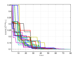
Figure 4: Time evolution of $\mathrm{RMSE}[\hat{b}^{\text{hom}}_{i}(t)]$ under time-varying communication graph. The solid lines indicate the theoretical expressions, while the dash-dot lines are the ones obtained via Monte Carlo simulations. The dashed horizontal line is the theoretical consensus value.

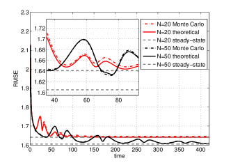
Figure 5: Time evolution of $\mathrm{RMSE}[\hat{\lambda}^{\text{ad-hoc}}_{i}(t)]$ under fixed communication graph for $N=20$ (red lines) and $N=50$ (black lines). The solid lines indicate the theoretical expressions, while the dash-dot lines are the ones obtained via Monte Carlo simulations. The dashed horizontal lines are the theoretical steady-state values.

Now we focus on the transient behavior of $\mathrm{RMSE}[\hat{\lambda}^{\text{ad-hoc}}_{i}(t)]$ for a generic node $i$. Notice that we use the index $i$, rather than $j$, meaning that in the Monte Carlo trials the node under investigation participates to the computation of $\hat{b}^{\text{hom}}_{i}(t)$. This allows us to show that the uncorrelation assumption in Section IV is in fact reasonable. Moreover, the computations will also confirm the validity of the low-order approximation made to derive the theoretical expressions of mean and variance.

In Figure 5 we compare the theoretical and sample evolution of $\mathrm{RMSE}[\hat{\lambda}^{\text{ad-hoc}}_{i}(t)]$. The theoretical curve is obtained by plugging equations (20) and (21) into equation (V). We compute the curves for two different values of $N$, namely $N=20$ and $N=50$. The difference between the theoretical and sample curves is already minimal for $N=20$ (showing a very weak correlation between $\hat{b}^{\text{hom}}_{i}(t)$ and $\sigma_{i}$) and completely disappears for $N=50$ (showing that the correlation has practically no more influence). We want to stress that running the same computation for a node not participating to the distributed computation (hence matching the uncorrelation assumption) the theoretical and sample curves are indistinguishable even for $N=20$. This suggests that the low-order approximation does not affect the goodness of the prediction.

It is worth noting that by increasing $N$ the steady-state value, $\mathrm{RMSE}[\hat{\lambda}^{\text{ad-hoc}}_{i}]$, decreases, since the hyperparameter $b$ is estimated by means of a larger sample. This aspect will be better highlighted in the following asymptotic analysis in which we focus on how $\mathrm{RMSE}[\hat{\lambda}^{\text{ad-hoc}}_{i}]$ varies with $N$.

In the asymptotic analysis we consider both the Empirical Bayes distributed estimator and the ad-hoc distributed estimator  by comparing again the predicted theoretical values with the sample counterparts. As in the transient analysis we first focus on the estimation of $b$.

In Figure 6 we plot the sample RMSE of the two estimators (ML and homogeneous) and compare them with the theoretical value of the homogeneous estimator and with the Cramer-Rao Bound (CRB). As expected, for each fixed $N$ the RMSE of the ML estimator is lower than the homogeneous one due to the (strong) inhomogeneity of the network. Once again, we recall that the homogeneous estimator coincides with the ML estimator only when the network is homogeneous (i.e., $n_{i}=n/N$ for any $i\in\{1,\dots,N\}$). As already experienced in the transient analysis, the theoretical values of $\mathrm{RMSE}[\hat{b}^{\text{hom}}]$ practically coincide with the sample ones. Although for the ML estimator we have no theoretical expression for fixed $N$, the picture shows a very interesting property. That is, the ML estimator achieves the CRB not only asymptotically ($N\rightarrow\infty$) as predicted by the theory, but also for each fixed $N$. Interestingly, in accordance to the theoretical results in the previous section, also the homogeneous estimator achieves the CRB as $N$ goes to infinity.

Finally, we analyze the RMSE of the estimators of $\lambda_{i}$. We consider an agent with one measurement ($n_{i}=1$) and use the most frequent value for the arrival rate, i.e., the mode of the Gamma distribution, $\lambda_{i}=(a-1)b$.

In Figure 7 we plot the sample RMSE of the Empirical Bayes and ad-hoc estimators. We also plot the (sample) values of the decentralized estimator. We decided to normalize all the curves to the theoretical value of the decentralized estimator in order to highlight the improvements of the proposed distributed estimators. Clearly, the sample values of the decentralized estimator are approximately equal to one, with minor fluctuations only due to the finite number of samples. We compare the sample curves with the theoretical curve of the homogeneous estimator and with the theoretical asymptotic value as $N\rightarrow\infty$. The theoretical curve is obtained as follows: $\mathrm{E}[\hat{\lambda}^{\text{ad-hoc}}_{i}]$ and $\mathrm{VAR}[\hat{\lambda}^{\text{ad-hoc}}_{i}]$ can be computed by plugging $\mathrm{VAR}[\hat{b}^{\text{hom}}]$ from (15) in (20) and (21); then, $\mathrm{RMSE}[\hat{\lambda}^{\text{ad-hoc}}_{i}]$ is obtained by plugging $\mathrm{E}[\hat{\lambda}^{\text{ad-hoc}}_{i}]$ and $\mathrm{VAR}[\hat{\lambda}^{\text{ad-hoc}}_{i}]$ into (V).

Again, although computed under the uncorrelation assumption and neglecting higher order terms, the theoretical expression $\mathrm{RMSE}[\hat{\lambda}^{\text{ad-hoc}}_{i}]$ predicts very accurately the sample values (cross markers and solid curve).

The plot confirms how the distributed estimators take advantage from the network growth although the local sample remains constant (even $n_{i}=1$). Indeed, the RMSE decreases as $N$ grows. The Empirical Bayes distributed estimator, being the optimal estimator, always outperforms the ad-hoc distributed estimator. However, as predicted by the theoretical analysis, the two estimators achieve the same asymptotic limit as $N\rightarrow\infty$. Moreover, it is interesting to notice that the RMSE of the two estimators practically coincide already for $N=16$, thus strengthening the already appealing features of the ad-hoc distributed estimator found from the theoretical analysis (i.e., easier computation and asymptotic optimality).

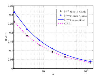
Figure 6: Sample RMSE for the homogeneous (triangles markers) and ML (circles markers) estimators of $b$ as a function of the number of agents $N$. The sample values are compared with the Cramer-Rao Bound (dashed line) and the theoretical RMSE of the homogeneous estimator (solid line).

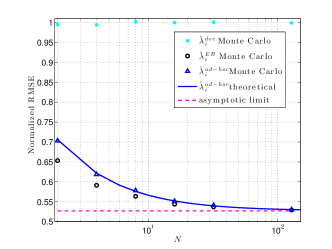
Figure 7: Sample RMSE for the ad-hoc (triangle markers) and Empirical Bayes (circle markers) estimators normalized with respect to the decentralized estimator of $\lambda_{i}$ (dot markers) as a function of the number of agents $N$. The theoretical RMSE of the ad-hoc estimator (solid line) and the theoretical limit (dashed line) are shown for comparison.

VI Conclusions

In this paper we have proposed a novel distributed scheme, based on a hierarchical framework, for the Bayesian estimation of arrival rates in asynchronous monitoring networks. The proposed distributed approach allows each node to gain information from the network and thus outperforms the decentralized estimator, especially when the node local information is scarce. In particular, the distributed estimator consists of the convex combination of a global information, computed through a distributed optimization algorithm, and a function of the local data. Then we have proposed an ad-hoc distributed estimator  that performs closely to the optimal Empirical Bayes estimator, but is much simpler to implement and exhibits faster (exponential) convergence. We have analyzed the two estimators and provided expressions for mean and variance as the network size goes to infinity, showing that in this asymptotic situation the ad-hoc estimator achieves the same RMSE of the optimal one. Moreover, for the ad-hoc estimator we have provided transient expressions for mean and variance. A numerical Monte Carlo analysis has been performed to corroborate the theoretical results and highlight the interesting features of the two distributed estimators.

-A Proof of Lemma 10

The Cramer-Rao Bound is defined as $\mathrm{CRB}(b)=\frac{1}{I(b)}$, where $I(b)$ is the Fisher Information. The Fisher Information is obtained from the likelihood (3) as:

$$I(b)=-\mathrm{E}\left[\frac{\partial^{2}\log L(\bm{y}_{1},\ldots,\bm{y}_{N}|b)}{\partial b^{2}}\right],$$

and, computing the derivatives,

$$I(b) =-\mathrm{E}\left[\frac{aN}{b^{2}}-\sum_{i=1}^{N}\frac{2n_{i}b+1}{b^{2}(n_{i}b+1)^{2}}(\sigma_{i}+a)\right]$$

$$=-\frac{aN}{b^{2}}+\sum_{i=1}^{N}\frac{2n_{i}b+1}{b^{2}(n_{i}b+1)^{2}}(\mathrm{E}\left[\sigma_{i}\right]+a).$$

Now, the mean of $\sigma_{i}$ turns out to be $\mathrm{E}[\sigma_{i}]=\mathrm{E}[\mathrm{E}[\sigma_{i}|\lambda_{i}]]=\mathrm{E}[n_{i}\lambda_{i}]=n_{i}ab$, so that, after some manipulation

$$I(b) =\frac{a}{b^{2}}\sum_{i=1}^{N}\left[-1+\frac{2n_{i}b+1}{(n_{i}b+1)^{2}}(n_{i}b+1)\right]$$

$$=\frac{a}{b^{2}}\sum_{i=1}^{N}\frac{n_{i}b}{n_{i}b+1},$$

so that the proof follows.

-B Proof of Theorem IV.2

The MMSE estimator of $\lambda_{j}$ in (11) can be written as $\hat{\lambda}^{\text{EB}}_{j}=Z(\hat{b}^{\text{ML}})Y(\sigma_{j})$, where $Z(\hat{b}^{\text{ML}})\stackrel{{\scriptstyle\textrm{\tiny def}}}{{=}}\frac{\hat{b}^{\text{ML}}}{1+\hat{b}^{\text{ML}}n_{j}}$ and $Y(\sigma_{j})\stackrel{{\scriptstyle\textrm{\tiny def}}}{{=}}a+\sigma_{j}$. Due to the independence between $\hat{b}^{\text{ML}}$ and $\sigma_{j}$, we have

$$\mathrm{E}[\hat{\lambda}^{\text{EB}}_{j}|\lambda_{j}]=\mathrm{E}[ZY|\lambda_{j}]=\mathrm{E}[Z|\lambda_{j}]\mathrm{E}[Y|\lambda_{j}]$$ (25)

and

$$\!\!\!\!\mathrm{VAR}[\hat{\lambda}^{\text{EB}}_{j}|\lambda_{j}] =\mathrm{E}^{2}[Z|\lambda_{j}]\mathrm{VAR}[Y|\lambda_{j}]$$

$$\quad+\!\mathrm{VAR}[Z|\lambda_{j}](\mathrm{E}^{2}[Y|\lambda_{j}]+\mathrm{VAR}[Y|\lambda_{j}]).$$ (26)

The conditional moments of $Y(\sigma_{j})$ are easily obtained

$$\mathrm{E}[Y(\sigma_{j})|\lambda_{j}]=a+n_{j}\lambda_{j}$$ (27)

and

$$\mathrm{VAR}[Y(\sigma_{j})|\lambda_{j}]=n_{j}\lambda_{j}.$$ (28)

For the nonlinear function $Z(\hat{b}^{\text{ML}})$ we resort to an approximate analysis. That is, we consider the Taylor expansion for the moments of the function $Z(\hat{b}^{\text{ML}})\stackrel{{\scriptstyle\textrm{\tiny def}}}{{=}}\frac{\hat{b}^{\text{ML}}}{1+\hat{b}^{\text{ML}}n_{j}}$ around the mean value $\mathrm{E}[\hat{b}^{\text{ML}}|\lambda_{j}]=\mathrm{E}[\hat{b}^{\text{ML}}]$.

$$\!\!\!\mathrm{E}[Z(\hat{b}^{\text{ML}})|\lambda_{j}] =\mathrm{E}[Z(\hat{b}^{\text{ML}})]$$

$$\approx\mathrm{E}\Big{[}Z(\mathrm{E}[\hat{b}^{\text{ML}}])+Z^{\prime}(\mathrm{E}[\hat{b}^{\text{ML}}])(\hat{b}^{\text{ML}}-\mathrm{E}[\hat{b}^{\text{ML}}])$$

$$\qquad+\frac{1}{2}Z^{\prime\prime}(\mathrm{E}[\hat{b}^{\text{ML}}])(\hat{b}^{\text{ML}}-\mathrm{E}[\hat{b}^{\text{ML}}])^{2}\Big{]},$$ (29)

where we have neglected terms of order higher than two in the expansion of $Z$, hence the $\approx$ symbol. Then

$$\mathrm{E}[Z(\hat{b}^{\text{ML}})|\lambda_{j}]\approx Z(\mathrm{E}[\hat{b}^{\text{ML}}])+\frac{1}{2}Z^{\prime\prime}(\mathrm{E}[\hat{b}^{\text{ML}}])\mathrm{VAR}[\hat{b}^{\text{ML}}].$$ (30)

Observing that $Z^{\prime}(s)=\frac{1}{(1+n_{j}s)^{2}}$ and $Z^{\prime\prime}(s)=-\frac{2n_{j}}{(1+n_{j}s)^{3}}$, and plugging (27) and (30) in (25), we get

$$\mathrm{E}[ \hat{\lambda}^{\text{EB}}_{j}|\lambda_{j}]\approx$$

$$(a+n_{j}\lambda_{j})\left[\frac{\mathrm{E}[\hat{b}^{\text{ML}}]}{\mathrm{E}[\hat{b}^{\text{ML}}]n_{j}+1}-\frac{n_{j}}{(\mathrm{E}[\hat{b}^{\text{ML}}]n_{j}+1)^{3}}\mathrm{VAR}[\hat{b}^{\text{ML}}]\right]\!.$$

From the asymptotic properties of the ML estimators, we know that for $N\rightarrow\infty$, $\mathrm{E}[\hat{b}^{\text{ML}}]\rightarrow b$ and $\mathrm{VAR}[\hat{b}^{\text{ML}}]\rightarrow 0$, so that equation (13) follows.

Similarly, it turns out that

$$\mathrm{VAR}[Z(\hat{b}^{\text{ML}})|\lambda_{j}] \approx\left(Z^{\prime\prime}(\mathrm{E}[\hat{b}^{\text{ML}}])\right)^{2}\mathrm{VAR}[\hat{b}^{\text{ML}}].$$ (31)

Using (30)-(31) into eq. (26) we obtain

$$\mathrm{VAR}[\hat{\lambda}^{\text{EB}}_{j}|\lambda_{j}]\approx\left(\frac{\mathrm{E}[\hat{b}^{\text{ML}}]}{\mathrm{E}[\hat{b}^{\text{ML}}]n_{j}+1}\right)^{2}n_{j}\lambda_{j}$$

$$\quad+\left[\frac{2n_{j}}{(\mathrm{E}[\hat{b}^{\text{ML}}]n_{j}+1)^{3}}\right]^{2}\mathrm{VAR}[\hat{b}^{\text{ML}}]\left[(a+n_{j}\lambda_{j})^{2}+n_{j}\lambda_{j}\right]\!.$$

Using again the asymptotic properties of $\hat{b}^{\text{ML}}$, equation (14) follows, thus concluding the proof.

-C Proof of Proposition IV.3

First, notice that $\mathrm{E}[\sigma_{i}|\lambda_{i}]=n_{i}\lambda_{i}$, thus

$$\mathrm{E}[\sigma] =\mathrm{E}[\mathrm{E}[\sigma|\bm{\lambda}]]=\mathrm{E}\left[\sum_{i=1}^{N}\mathrm{E}[\sigma_{i}|\lambda_{i}]\right]=\mathrm{E}\left[\sum_{i=1}^{N}n_{i}\lambda_{i}\right]$$

$$=\sum_{i=1}^{N}n_{i}ab=nab,$$

so that $\mathrm{E}[\hat{b}^{\text{hom}}]=b$.

To prove the second part, recall that $\mathrm{VAR}[\sigma_{i}|\lambda_{i}]=n_{i}\lambda_{i}$ and, thus, $\mathrm{VAR}[\sigma|\bm{\lambda}]=\sum_{i=1}^{N}\mathrm{VAR}[\sigma_{i}|\lambda_{i}]=\sum_{i=1}^{N}n_{i}\lambda_{i}$. Using the law of total variance, we have

$$\begin{split}\mathrm{VAR}[\sigma]&=\mathrm{E}[\mathrm{VAR}[\sigma|\bm{\lambda}]]+\mathrm{VAR}[\mathrm{E}[\sigma|\bm{\lambda}]]\\ &=\mathrm{E}\left[\sum_{i=1}^{N}\mathrm{VAR}[\sigma_{i}|\lambda_{i}]\right]+\mathrm{VAR}\left[\sum_{i=1}^{N}\mathrm{E}[\sigma_{i}|\lambda_{i}]\right]\\ &=\mathrm{E}\left[\sum_{i=1}^{N}n_{i}\lambda_{i}\right]+\mathrm{VAR}\left[\sum_{i=1}^{N}n_{i}\lambda_{i}\right]\\ &=abn+ab^{2}\sum_{i=1}^{N}n_{i}^{2}.\end{split}$$

The variance of the homogeneous estimator is given by $\mathrm{VAR}[\hat{b}^{\text{hom}}]=\mathrm{VAR}\left[\frac{\sigma}{an}\right]$, so that equation (15) follows.

By Markov’s inequality and Lemma IV.3

$$\mathrm{Pr}\left\{\left|\frac{\sigma}{an}-b\right|\geq\epsilon\right\}\leq\frac{1}{\epsilon}\mathrm{VAR}\left[\hat{b}^{\text{hom}}\right],$$

and the variance can be bounded as follows

$$\begin{split}\mathrm{VAR}\left[\hat{b}^{\text{hom}}\right]&=\frac{b}{an}+\frac{b^{2}}{an^{2}}\sum_{i=1}^{N}n_{i}^{2}\\ &\leq\frac{b}{aN}+\frac{b^{2}}{aN^{2}}\sum_{i=1}^{N}n_{\text{max}}^{2}\\ &=\frac{b}{aN}+\frac{{n_{\text{max}}}^{2}b^{2}}{aN}\;\stackrel{{\scriptstyle N\rightarrow\infty}}{{\xrightarrow{\hskip 28.45274pt}}}\;0\end{split}$$

so that $\hat{b}^{\text{hom}}\rightarrow b$ in probability, thus concluding the proof.

-D Proof of Lemma IV.5

To prove that $\hat{b}^{\text{hom}}_{i}(t)$ is unbiased at any $t\in{\mathbb{Z}_{\geq 0}}$, first let us recall that the aggregate states $\eta(t)=[\eta_{1}(t)\ldots\eta_{N}(t)]^{T}$ and $s(t)=[s_{1}(t)\ldots s_{N}(t)]^{T}$ evolve according to the dynamics (7) with $s(0)=[\sigma_{1}\ldots\sigma_{N}]^{T}\stackrel{{\scriptstyle\textrm{\tiny def}}}{{=}}\bm{\sigma}$, $\eta(0)=[n_{1}\ldots n_{N}]^{T}\stackrel{{\scriptstyle\textrm{\tiny def}}}{{=}}\bm{n}$ and $W(t)$ the column stochastic matrix with elements $w_{ij}(t)$. The evolution of $s(t)$ and $\eta(t)$ is given by (9) where $\Phi(t)$ is the deterministic state transition matrix defined in (8).

Next, observe that the update $\eta_{i}(t)$ depends only on the initial value $n_{i}$ and thus is deterministic. Therefore, using the update in Algorithm 2, we have

$$\mathrm{E}[\hat{b}^{\text{hom}}_{i}(t)]=\frac{1}{a\eta_{i}(t)}\mathrm{E}[s_{i}(t)]$$

Using the evolution of the aggregate state and denoting $e_{i}$ the $i$th canonical vector (e.g., $e_{1}=[1\;0\;\ldots\;0]^{T}$), we have

$$\begin{split}\mathrm{E}[\hat{b}^{\text{hom}}_{i}(t)]&=\frac{1}{a\eta_{i}(t)}\mathrm{E}[e_{i}^{T}(\Phi(t)\bm{\sigma})]\\ &=\frac{1}{a\eta_{i}(t)}e_{i}^{T}\Phi(t)\mathrm{E}[\bm{\sigma}].\end{split}$$

Noting that $\mathrm{E}[\sigma_{i}]=abn_{i}$ it follows

$$\begin{split}\mathrm{E}[\hat{b}^{\text{hom}}_{i}(t)]&=\frac{1}{a\eta_{i}(t)}e_{i}^{T}\Phi(t)ab\,\bm{n}\\ &=\frac{b}{\eta_{i}(t)}e_{i}^{T}\eta(t)=b\\ \end{split}$$

where the last two steps follow respectively from (9) ($\Phi(t)\bm{n}=\eta(t)$) and from $e_{i}^{T}\eta(t)=\eta_{i}(t)$.

Next, we show that the transient variance is given by equation (16).

Using again the update in Algorithm 2, it holds

$$\begin{split}\mathrm{VAR}[\hat{b}^{\text{hom}}_{i}(t)]&=\frac{1}{a^{2}\eta_{i}(t)^{2}}\mathrm{VAR}[e_{i}^{T}(\Phi(t)\bm{\sigma})].\\ \end{split}$$

Noting that $e_{i}^{T}\Phi(t)$ is the $i$th row of $\Phi(t)$, it follows

$$\begin{split}\mathrm{VAR}[\hat{b}^{\text{hom}}_{i}(t)]&=\frac{1}{a^{2}\eta_{i}(t)^{2}}\mathrm{VAR}\left[\sum_{k=1}^{N}\phi_{ik}(t)\sigma_{k}\right],\end{split}$$

where $\phi_{ik}(t)$ is the element $(i,k)$ of the matrix $\Phi(t)$. By the law of total variance we have that

$$\begin{split}\mathrm{VAR}[\hat{b}^{\text{hom}}_{i}(t)]&=\frac{1}{a^{2}\eta_{i}(t)^{2}}\left\{\mathrm{E}\left[\mathrm{VAR}\left[\sum_{k=1}^{N}\phi_{ik}(t)\sigma_{k}\;\Big{|}\;\bm{\lambda}\right]\right]\right.\\ &\qquad\left.+\mathrm{VAR}\left[\mathrm{E}\left[\sum_{k=1}^{N}\phi_{ik}(t)\sigma_{k}\;\Big{|}\;\bm{\lambda}\right]\right]\right\}\\ &=\frac{1}{a^{2}\eta_{i}(t)^{2}}\left\{\mathrm{E}\left[\sum_{k=1}^{N}\phi_{ik}(t)^{2}n_{k}\lambda_{k}\right]\right.\\ &\left.\qquad+\mathrm{VAR}\left[\sum_{k=1}^{N}\phi_{ik}(t)n_{k}\lambda_{k}\right]\right\},\end{split}$$

where we have used $\mathrm{E}[\sigma_{k}]=n_{k}\lambda_{k}$ and $\mathrm{VAR}[\sigma_{k}]=n_{k}\lambda_{k}$. Finally, recalling that $\mathrm{E}[\lambda_{k}]=ab$, $\mathrm{VAR}[\lambda_{k}]=ab^{2}$ and the $\lambda_{k}$s are independent, it turns out

$$\begin{split}\mathrm{VAR}[\hat{b}^{\text{hom}}_{i}(t)]&=\frac{b}{a\eta_{i}(t)^{2}}\left(\sum_{k=1}^{N}\phi_{ik}(t)^{2}n_{k}+b\sum_{k=1}^{N}\phi_{ik}(t)^{2}n_{k}^{2}\right),\end{split}$$

so that equation (16) follows.

To prove the asymptotic result, we work out $|\mathrm{VAR}[\hat{b}^{\text{hom}}_{i}(t)]-\mathrm{VAR}[\hat{b}^{\text{hom}}]|$ by using (16) and (15)

$$\begin{split}|&\mathrm{VAR}[\hat{b}^{\text{hom}}_{i}(t)]-\mathrm{VAR}[\hat{b}^{\text{hom}}]|=\\ &=\left|\frac{b}{a}\left(\frac{\sum_{k=1}^{N}\phi_{ik}(t)^{2}n_{k}}{{\left(\sum_{k=1}^{N}\phi_{ik}(t)n_{k}\right)^{2}}}-\frac{1}{n}\right)\right.\\ &\qquad\left.+\frac{b^{2}}{a}\left(\frac{\sum_{k=1}^{N}\phi_{ik}(t)^{2}n_{k}^{2}}{\left(\sum_{k=1}^{N}\phi_{ik}(t)n_{k}\right)^{2}}-\frac{\sum_{k=1}^{N}n_{k}^{2}}{n^{2}}\right)\right|\\ &=\frac{1}{\eta_{i}(t)^{2}}\left|\frac{b}{an}\left(n\sum_{k=1}^{N}\phi_{ik}(t)^{2}n_{k}-\left(\sum_{k=1}^{N}\phi_{ik}(t)n_{k}\right)^{2}\right)\right.\\ &\qquad\left.+\frac{b^{2}}{an^{2}}\left(n^{2}\sum_{k=1}^{N}\phi_{ik}(t)^{2}n_{k}^{2}-\left(\sum_{k=1}^{N}\phi_{ik}(t)n_{k}\right)^{2}\sum_{k=1}^{N}n_{k}^{2}\right)\!\right|\\ \end{split}$$

By using the definition of $n=\sum_{h=1}^{N}n_{h}$ and writing $\left(\sum_{k=1}^{N}\phi_{ik}(t)n_{k}\right)^{2}=\left(\sum_{k=1}^{N}\phi_{ik}(t)n_{k}\right)\left(\sum_{h=1}^{N}\phi_{ih}(t)n_{h}\right)$

$$\begin{split}|&\mathrm{VAR}[\hat{b}^{\text{hom}}_{i}(t)]-\mathrm{VAR}[\hat{b}^{\text{hom}}]|=\\ &=\frac{1}{\eta_{i}(t)^{2}}\left|\frac{b}{an}\left(\sum_{h=1}^{N}n_{h}\sum_{k=1}^{N}\phi_{ik}(t)^{2}n_{k}\right.\right.\\ &\qquad\left.-\sum_{k=1}^{N}\phi_{ik}(t)n_{k}\sum_{h=1}^{N}\phi_{ih}(t)n_{h}\right)\\ &\qquad+\frac{b^{2}}{an^{2}}\left(\sum_{h=1}^{N}n_{h}\sum_{\ell=1}^{N}n_{\ell}\sum_{k=1}^{N}\phi_{ik}(t)^{2}n_{k}^{2}\right.\\ &\qquad\left.\left.-\sum_{h=1}^{N}\phi_{ih}(t)n_{h}\sum_{\ell=1}^{N}\phi_{i\ell}(t)n_{\ell}\sum_{k=1}^{N}n_{k}^{2}\right)\right|\\ &=\frac{1}{\eta_{i}(t)^{2}}\Bigg{|}\frac{b}{an}\sum_{h=1}^{N}\sum_{k=1}^{N}n_{h}n_{k}\phi_{ik}(t)\left(\phi_{ik}(t)-\phi_{ih}(t)\right)\\ &\qquad+\frac{b^{2}}{an^{2}}\sum_{h=1}^{N}\sum_{\ell=1}^{N}\sum_{k=1}^{N}n_{h}n_{\ell}n_{k}^{2}\left(\phi_{ik}(t)^{2}-\phi_{ih}(t)\phi_{i\ell}(t)\right.\\ &\qquad+\left.\phi_{ik}(t)\phi_{i\ell}(t)-\phi_{ik}(t)\phi_{i\ell}(t)\right)\Bigg{|}\\ &\leq\frac{1}{\eta_{i}(t)^{2}}\Bigg{[}\frac{b}{an}\sum_{h=1}^{N}\sum_{k=1}^{N}n_{h}n_{k}\phi_{ik}(t)\left|\phi_{ik}(t)-\phi_{ih}(t)\right|\\ &\qquad+\frac{b^{2}}{an^{2}}\sum_{h=1}^{N}\sum_{\ell=1}^{N}\sum_{k=1}^{N}n_{h}n_{\ell}n_{k}^{2}\phi_{ik}(t)\Big{(}\left|\phi_{ik}(t)-\phi_{ih}(t)\right|\\ &\qquad+\left|\phi_{ik}-\phi_{i\ell}(t)\right|\Big{)}\Bigg{]}\end{split}$$

where the last inequality follows by using the triangular inequality. Now, weak ergodicity of $W(t)$ implies that for any $i,k,h\in\{1,\dots,N\}$ it holds $\left|\phi_{ik}(t)-\phi_{ih}(t)\right|\leq M\lambda^{t}$ for some $M>0$ and $\lambda>0$, see, e.g., [13, Corollary 8], so that the exponential convergence of $\mathrm{VAR}[\hat{b}^{\text{hom}}_{i}(t)]$ follows. Then, from the definition of the coefficient of ergodicity, it follows

$$| \mathrm{VAR}[\hat{b}^{\text{hom}}_{i}(t)]-\mathrm{VAR}[\hat{b}^{\text{hom}}]|$$

$$\leq\frac{1}{\sum_{k=1}^{N}\phi_{ik}(t)n_{k}}\left(\frac{b}{an}n\delta(\Phi(t))+\frac{b^{2}}{an^{2}}n^{2}n_{\text{max}}2\delta(\Phi(t))\right)$$

where we have simplified the common factor $\eta_{i}(t)=\sum_{k=1}^{N}\phi_{ik}(t)n_{k}$. Finally, by Lemma III.4, $\sum_{k=1}^{N}\phi_{ik}(t)\geq\mu$, with $\mu>0$ so that

$$|\mathrm{VAR}[\hat{b}^{\text{hom}}_{i}(t)]-\mathrm{VAR}[\hat{b}^{\text{hom}}]| \leq\frac{\delta(\Phi(t))b(1+2bn_{\text{max}})}{\mu a}$$

thus concluding the proof.

-E Proof of Theorem IV.8

The local update of the ad-hoc distributed estimator  (Algorithm 2) can be written as $\hat{\lambda}^{\text{ad-hoc}}_{j}(t)=X(\hat{b}^{\text{hom}}_{j}(t))Y(\sigma_{j})$, where $X(\hat{b}^{\text{hom}}_{j}(t))\stackrel{{\scriptstyle\textrm{\tiny def}}}{{=}}\frac{\hat{b}^{\text{hom}}_{j}(t)}{1+\hat{b}^{\text{hom}}_{j}(t)n_{j}}$ and $Y(\sigma_{j})\stackrel{{\scriptstyle\textrm{\tiny def}}}{{=}}a+\sigma_{j}$. Using again the independence between $\hat{b}^{\text{hom}}_{j}(t)$ and $\sigma_{j}$, we can write $\mathrm{E}[\hat{\lambda}^{\text{ad-hoc}}_{j}(t)|\lambda_{j}]$ and $\mathrm{VAR}[\hat{\lambda}^{\text{ad-hoc}}_{j}(t)|\lambda_{j}]$ as

$$\mathrm{E}[\hat{\lambda}^{\text{ad-hoc}}_{j}(t)|\lambda_{j}]=\mathrm{E}[XY|\lambda_{j}]=\mathrm{E}[X|\lambda_{j}]\mathrm{E}[Y|\lambda_{j}]$$ (32)

and

$$\!\!\!\mathrm{VAR}[\hat{\lambda}^{\text{ad-hoc}}_{j}(t) |\lambda_{j}]=\mathrm{E}^{2}[X|\lambda_{j}]\mathrm{VAR}[Y|\lambda_{j}]$$

$$+\mathrm{VAR}[X|\lambda_{j}](\mathrm{E}^{2}[Y|\lambda_{j}]\!+\!\mathrm{VAR}[Y|\lambda_{j}]).$$ (33)

Considering, as in the previous theorem, the Taylor expansion for the moments of the function $X(\hat{b}^{\text{hom}}_{j}(t))\stackrel{{\scriptstyle\textrm{\tiny def}}}{{=}}\frac{\hat{b}^{\text{hom}}_{j}(t)}{1+\hat{b}^{\text{hom}}_{j}(t)n_{j}}$ around the mean $\mathrm{E}[\hat{b}^{\text{hom}}_{j}(t)|\lambda_{j}]=b$, we obtain

$$\mathrm{E}[X( \hat{b}^{\text{hom}}_{j}(t))|\lambda_{j}]=\mathrm{E}[X(\hat{b}^{\text{hom}}_{j}(t))]$$

$$\approx X(\mathrm{E}[\hat{b}^{\text{hom}}_{j}(t)])+\frac{1}{2}X^{\prime\prime}(\mathrm{E}[\hat{b}^{\text{hom}}_{j}(t)])\mathrm{VAR}[\hat{b}^{\text{hom}}_{j}(t)]$$

$$=\frac{b}{1+n_{j}b}-\frac{n_{j}}{(1+n_{j}b)^{3}}\mathrm{VAR}[\hat{b}^{\text{hom}}_{j}(t)]$$ (34)

where $\mathrm{VAR}[\hat{b}^{\text{hom}}_{j}(t)]$ is the one given in (16) and, again, the $\approx$ symbol indicates that we have neglected higher-order terms in the expansion of $X$. Hence, plugging (27) and (34) in (32), equation (20) follows. Similarly,

$$\mathrm{VAR}[X( \hat{b}^{\text{hom}}_{j}(t))|\lambda_{j}]\approx\left(X^{\prime}(\mathrm{E}[\hat{b}^{\text{hom}}_{j}(t)])\right)^{2}\mathrm{VAR}[\hat{b}^{\text{hom}}_{j}(t)]$$

$$=\left[\frac{1}{(1+n_{j}b)^{2}}\right]^{2}\left(\frac{b}{an}+\frac{b^{2}}{an^{2}}\sum_{i=1}^{N}n_{i}^{2}\right).$$ (35)

Using (34)-(35) into (33), equation (21) follows, thus concluding the first part of the proof.

To prove the asymptotic results, we just need to recall from Proposition IV.3 that as $N\rightarrow\infty$ $\mathrm{VAR}[\hat{b}^{\text{hom}}]\rightarrow 0$, so that equations (22) and (23) follow, thus concluding the proof.

Angelo Coluccia (M’13) received the Eng. degree in Telecommunication Engineering (summa cum laude) in 2007 and the PhD degree in Information Engineering in 2011, both from the University of Salento, Lecce, Italy. Former researcher at Forschungszentrum Telekommunikation Wien, Vienna, since 2008 he has been engaged in research projects on traffic analysis, security and anomaly detection in operational cellular networks. He is currently Assistant Professor at the Dipartimento di Ingegneria dell’Innovazione, University of Salento, where he teaches the course of Telecommunication Systems. His research interests are signal processing, communications and wireless networks, in particular cooperative sensing/estimation approaches for localization and other (possibly distributed) applications.

Giuseppe Notarstefano has been an Assistant Professor (Ricercatore) at the Università del Salento (Lecce, Italy) since February 2007. He received the Laurea degree “summa cum laude” in Electronics Engineering from the Università di Pisa in 2003 and the Ph.D. degree in Automation and Operation Research from the Università di Padova in April 2007. He has been visiting scholar at the Universities of Stuttgart, California Santa Barbara and Colorado Boulder. His research interests include distributed optimization, cooperative control in multi-agent networks, applied nonlinear optimal control, and trajectory optimization and maneuvering of aerial and car vehicles. He serves as an Associate Editor in the Conference Editorial Board of the IEEE Control Systems Society and for the European Control Conference, IFAC World Congress and IEEE Multi-Conference on Systems and Control. He coordinated the VI-RTUS team winning the International Student Competition Virtual Formula 2012. He is recipient of an ERC Starting Grant 2014.

References

• [1] A. Coluccia and G. Notarstefano, “Distributed bayesian estimation of arrival rates in asynchronous monitoring networks,” in IEEE International Conference on Acoustics, Speech and Signal Processing (ICASSP), 2014, pp. 5050–5054.
• [2] D. L. Snyder and M. I. Miller, Random Point Processes in Time and Space.   Springer, 1991.
• [3] D. Heyman and M. Sobel, Stochastic Models in Operations Research: Stochastic optimization, ser. Dover Books on Computer Science Series.   Dover Publications, 2003.
• [4] S. Barbarossa, S. Sardellitti, and P. Di Lorenzo, Distributed detection and estimation in wireless sensor networks, ser. Communications and Radar Signal Processing.   Academic Press Library in Signal Processing, October 2013, vol. 2, ch. 7, pp. 329–408.
• [5] I. D. Schizas, A. Ribeiro, and G. B. Giannakis, “Consensus in ad hoc WSNs with noisy linksâ Part I: Distributed estimation of deterministic signals,” IEEE Transactions on Signal Processing, vol. 56, no. 1, pp. 350–364, 2008.
• [6] F. S. Cattivelli and A. H. Sayed, “Diffusion lms strategies for distributed estimation,” IEEE Transactions on Signal Processing, vol. 58, no. 3, pp. 1035–1048, 2010.
• [7] S. Barbarossa and G. Scutari, “Bio-inspired sensor network design,” IEEE Signal Processing Magazine, vol. 24, no. 3, pp. 26–35, 2007.
• [8] F. Garin and L. Schenato, “A survey on distributed estimation and control applications using linear consensus algorithms,” Networked Control Systems, pp. 75–107, 2011.
• [9] P. Frasca, H. Ishii, C. Ravazzi, and R. Tempo, “Distributed randomized algorithms for opinion formation, centrality computation and power systems estimation: A tutorial overview,” European Journal of Control, 2015.
• [10] S. Sardellitti, M. Giona, and S. Barbarossa, “Fast distributed average consensus algorithms based on advection-diffusion processes,” IEEE Transactions on Signal Processing, vol. 58, no. 2, 2010.
• [11] D. E. Marelli and M. Fu, “Distributed weighted least-squares estimation with fast convergence for large-scale systems,” Automatica, vol. 51, pp. 27–39, 2015.
• [12] F. Pasqualetti, R. Carli, and F. Bullo, “Distributed estimation via iterative projections with application to power network monitoring,” Automatica, vol. 48, no. 5, pp. 747–758, 2012.
• [13] A. Nedic and A. Olshevsky, “Distributed optimization over time-varying directed graphs,” arXiv preprint arXiv:1303.2289, 2013.
• [14] S. Barbarossa and G. Scutari, “Decentralized maximum-likelihood estimation for sensor networks composed of nonlinearly coupled dynamical systems,” IEEE Transactions on Signal Processing, vol. 55, no. 7, 2007.
• [15] A. Chiuso, F. Fagnani, L. Schenato, and S. Zampieri, “Gossip algorithms for simultaneous distributed estimation and classification in sensor networks,” IEEE Journal of Selected Topics in Signal Processing, vol. 5, no. 4, pp. 691–706, 2011.
• [16] F. Fagnani, S. M. Fosson, and C. Ravazzi, “Input driven consensus algorithm for distributed estimation and classification in sensor networks,” in 50th IEEE Conference on Decision and Control and European Control Conference (CDC-ECC).   IEEE, 2011, pp. 6654–6659.
• [17] D. Varagnolo, G. Pillonetto, and L. Schenato, “Distributed consensus-based bayesian estimation: sufficient conditions for performance characterization,” in American Control Conference.   IEEE, 2010, pp. 3986–3991.
• [18] P. Di Lorenzo and S. Barbarossa, “Distributed least mean squares strategies for sparsity-aware estimation over gaussian markov random fields,” in IEEE International Conference on Acoustics, Speech and Signal Processing (ICASSP), 2014, pp. 5472–5476.
• [19] F. Cattivelli, C. G. Lopes, and A. H. Sayed, “Diffusion recursive least-squares for distributed estimation over adaptive networks,” IEEE Transactions on Signal Processing, vol. 56, no. 5, 2008.
• [20] G. Mateos, I. D. Schizas, and G. B. Giannakis, “Distributed recursive least-squares for consensus-based in-network adaptive estimation,” IEEE Transactions on Signal Processing, vol. 57, no. 11, pp. 4583–4588, 2009.
• [21] I. D. Schizas, G. B. Giannakis, S. I. Roumeliotis, and A. Ribeiro, “Consensus in ad hoc WSNs with noisy linksâ Part II: Distributed estimation and smoothing of random signals,” IEEE Transactions on Signal Processing, vol. 56, no. 4, pp. 1650–1666, 2008.
• [22] D. A. Freedman, “Poisson processes with random arrival rate,” The Annals of Mathematical Statistics, pp. 924–929, 1962.
• [23] W. A. Massey, G. A. Parker, and W. Whitt, “Estimating the parameters of a nonhomogeneous poisson process with linear rate,” Telecommunication Systems, vol. 5, no. 2, pp. 361–388, 1996.
• [24] D. Karlis and E. Xekalaki, “Mixed poisson distributions,” International Statistical Review, vol. 73, pp. 35–58, 2005.
• [25] C. Withers and S. Nadarajah, “On the compound poisson-gamma distribution,” Kybernetika, vol. 47, no. 1, pp. 15–37, 2011.
• [26] E. Lehmann and G. Casella, Theory of Point Estimation.   Springer, 1998.
• [27] F. Zanella, D. Varagnolo, A. Cenedese, G. Pillonetto, and L. Schenato, “Asynchronous newton-raphson consensus for distributed convex optimization,” in 3rd IFAC Workshop on Distributed Estimation and Control in Networked Systems (NecSys’12), 2012.
• [28] J. N. Tsitsiklis, D. P. Bertsekas, M. Athans et al., “Distributed asynchronous deterministic and stochastic gradient optimization algorithms,” IEEE Transactions on Automatic Control, vol. 31, no. 9, pp. 803–812, 1986.
• [29] E. Seneta, Non-negative matrices and Markov chains.   Springer, 2006.
• [30] A. Jadbabaie, J. Lin, and A. S. Morse, “Coordination of groups of mobile autonomous agents using nearest neighbor rules,” IEEE Transactions on Automatic Control, vol. 48, no. 6, pp. 988–1001, 2003.
• [31] F. Bénézit, V. Blondel, P. Thiran, J. Tsitsiklis, and M. Vetterli, “Weighted gossip: Distributed averaging using non-doubly stochastic matrices,” in IEEE International Symposium on Information Theory Proceedings (ISIT).   IEEE, 2010, pp. 1753–1757.
• [32] N. H. Vaidya, C. N. Hadjicostis, and A. D. Dominguez-Garcia, “Distributed algorithms for consensus and coordination in the presence of packet-dropping communication links-part ii: Coefficients of ergodicity analysis approach,” arXiv preprint arXiv:1109.6392, 2011.