Benchmarking the computing resources at the Instituto de Astrofísica de Canarias Nicola Caon^1,2*, Antonio J. Dorta^1,2, Juan Carlos Trelles Arjona² Benchmarks — Supercomputing The aim of this study is the characterization of the computing resources used by researchers at the ”Instituto de Astrofísica de Canarias” (IAC). Since there is a huge demand of computing time and we use tools such as HTCondor to implement High Throughput Computing (HTC) across all available PCs, it is essential for us to assess in a quantitative way, using objective parameters, the performances of our computing nodes. In order to achieve that, we have run a set of benchmark tests on a number of different desktop and laptop PC models among those used in our institution. In particular, we run the ”Polyhedron Fortran Benchmarks” suite, using three different compilers: GNU Fortran Compiler, Intel Fortran Compiler and the PGI Fortran Compiler; execution times are then normalized to the reference values published by Polyhedron. The same tests were run multiple times on a same PCs, and on 3 to 5 PCs of the same model (whenever possible) to check for repeatability and consistency of the results. We found that in general execution times, for a given PC model, are consistent within an uncertainty of about 10%, and show a gain in CPU speed of a factor of about 3 between the oldest PCs used at the IAC (7-8 years old) and the newest ones.

1 The IAC computing resources

At the Instituto de Astrofísica de Canarias there are about 250 desktop PCs with Linux installed, used by scientists and engineers. These PCs cover a wide span of models and ages, from 8-years old Dell Optiplex to recently bought ”NausicaA” models. There are also several more powerful computers, mainly rack-mounted but also a few desktop models, dedicated to large, demanding jobs that exceed the capabilities of a ”regular” (consumer) PC, such as massive data reduction and analysis, simulations, and other CPU intensive jobs.

While it is clear that newer PCs are faster and more efficient than older models, so far this was more a perception than solid evidence supported by data. A user may observe that her office-mate’s latest-model PC is more responsive, or faster when executing some tasks, but cannot say by how much, nor can she estimates the gain in time obtained by running her applications in the office-mate’s PC instead of her own older PC. This could be a key factor when preparing the remote executions of a program using the available HTC tools, since it is possible to specify a list of preferences or ranks that will be used to choose the target machines on which the code will be executed.

For these reasons we decided to run a set of benchmarking tests on all the different, available desktop and rack models, with also a few laptops, as part of a month-long ”Proyecto Práctica de Empresa” (Student Internship), carried out at the IAC by a 4th-year student of Astronomy (JCTA).

2 Running the benchmark tools

2.1 The Polyhedron benchmarks suite

After considering a number of possible benchmarks, we finally selected the ”Polyhedron Fortran Benchmarks” suite [1], since it is one of the most comprehensive set of benchmarks that matches our requirements: it provides tools to automatically run the tests, compute the CPU time used by each executable, validate and save the results in tabular form in a simple text file.

This benchmark consists of 17 independent Fortran programs. While this suite was devised to compare the performances of 10 different Fortran compilers on a same machine, it can be used as well to compare the performances of a same compiler on a variety of hardware.

The way it operates is controlled by a couple of parameter files, one (general) listing the tests to be run, the desired accuracy to be achieved, the minimum and maximum number of runs for each test, and the maximum execution time permitted. (A detailed explanation of how the test suite works is provided in [2]). Then there is a parameter file tailored to each compiler, with the specific command and flags to be used.

We made only minor changes in the parameter files provided by Polyhedron, by increasing the tolerance on the execution time from 0.1 to 0.2, setting the maximum number of runs for each test to 20, and limiting the maximum execution time to 4000 seconds. These changes do not affect the reliability of our results, but allow a shorter overall time for running the whole suite of tests (typically from two to seven hours). The limits on the maximum number of tests and maximum execution time (per test) prevented jobs from getting out of control and using up the CPU for hours or even days (which happened a few times, especially with the Intel compiler).

To check the consistency of the results, we:
a) ran the benchmarks multiple times on a same machine, and
b) ran the tests on 3 to 5 different PCs of a same desktop model. However, we typically have only one single model of the more powerful machines dedicated to CPU-intensive jobs, so we could only perform the consistency check a). This same limitation applies to laptops.

Table 1 lists the hardware on which the Polyhedron test suite was run, together with the main data about their CPU and RAM.

Table 2 lists the compilers installed at the IAC and used for the benchmark tests. All the computers on which the tests were run had Linux Fedora 19 installed, and all have the same exact version of the three compilers used.

PC model	Type	Date	Processor Type	Cache	RAM	Number
Dell Precision WS T7400	Desktop	late 2007	Intel(R) Xeon(R) CPU X5472 @ 3.00GHz	6144 KB	32 GB	2
Dell Optiplex 740(a)	Desktop	late 2007	AMD Athlon(tm) 64 X2 Dual Core Processor 5200+	1024 KB	4 GB	5
Dell Optiplex 740(a)	Desktop	early 2008	AMD Athlon(tm) 64 X2 Dual Core Processor 5600+	512 KB	4 GB	4
Dell Optiplex 740(a)	Desktop	mid 2009	AMD Athlon(tm) 64 X2 Dual Core Processor 6000+	1024 KB	4 GB	5
Dell Optiplex 780(b)	Desktop	late 2009	Intel(R) Core(TM)2 Quad CPU Q9400 @ 2.66GHz	3072 KB	8 GB	8
Dell Optiplex 780(b)	Desktop	late 2009	Intel(R) Core(TM)2 Duo CPU E8400 @ 3.00GHz	3072 KB	8 GB	4
Dell Precision WS T3500	Desktop	early 2011	Intel(R) Xeon(R) CPU W3565 @ 3.20GHz	8192 KB	12 GB	1
Dell Precision WS T3600	Desktop	mid 2012	Intel(R) Xeon(R) CPU E5-1650 0 @ 3.20GHz	12288 KB	32 GB	1
Dell Precision WS T5600	Desktop	mid 2012	Intel(R) Xeon(R) CPU E5-2687W 0 @ 3.10GHz	20480 KB	128 GB	1
Dell Optiplex 7010	Desktop	mid 2012	Intel(R) Core(TM) i5-3470 CPU @ 3.20GHz	6144 KB	8 GB	5
ALDA+	Desktop	mid 2014	Intel(R) Core(TM) i7-4770 CPU @ 3.40GHz	8192 KB	8 GB	5
NausicaA	Desktop	mid 2014	Intel(R) Core(TM) i7-4790 CPU @ 3.60GHz	8192 KB	8 GB	4
Dell Precision WS T5400	Rack	late 2007	Intel(R) Xeon(R) CPU X5450 @ 3.00GHz	6144 KB	8 GB	1
Dell Precision WS-690	Rack	early 2008	Intel(R) Xeon(R) CPU X5355 @ 2.66GHz	4096 KB	32 GB	2
Dell PowerEdge-2970	Rack	late 2008	Quad-Core AMD Opteron(tm) Processor 2358 SE	512 KB	64 GB	1
Dell PowerEdge R410	Rack	late 2009	Intel(R) Xeon(R) CPU X5570 @ 2.93GHz	8192 KB	16 GB	1
Tecal RH5885 V3	Rack	mid 2014	Intel(R) Xeon(R) CPU E7-4820 v2 @ 2.00GHz	16384 KB	256 GB	1
Dell Latitude E6500	Laptop	mid 2008	Intel(R) Core(TM)2 Duo CPU T9400 @ 2.53GHz	6144 KB	4 GB	1
Dell Latitude E4200	Laptop	late 2008	Intel(R) Core(TM)2 Duo CPU U9600 @ 1.60GHz	3072 KB	3 GB	1
Dell Latitude E4300	Laptop	late 2008	Intel(R) Core(TM)2 Duo CPU P9300 @ 2.26GHz	6144 KB	4 GB	1
Dell Latitude E6320	Laptop	early 2011	Intel(R) Core(TM) i7-2720QM CPU @ 2.20GHz	6144 KB	4 GB	1
Dell Latitude E6520	Laptop	early 2011	Intel(R) Core(TM) i7-2620M CPU @ 2.70GHz	4096 KB	8 GB	2
Lenovo L440	Laptop	late 2014	Intel(R) Core(TM) i5-4200M CPU @ 2.50GHz	3072 KB	8 GB	1

Table 1: Column ”Date” show the production date of that specific model as retrieved from the corresponding Dell page [3] after supplying the service tag. For some of the models the Dell website does not provide useful information, so we listed the approximate time the PC model was bought (this also applies to non-Dell models).
Within each ”Type” group, the list is ordered chronologically.
^(a): The Dell Optiplex 740 model actually came with three CPU variants; ^(b): The Dell Optiplex 780 model actually came with two CPU variants. Column ”Number” shows the number of PCs of that model on which the benchmark tests were run.

compiler	version	compilation flags
gfortran	GNU Fortran (GCC) 4.8.3 20140911	-march=native -ffast-math -funroll-loops -O3
Intel	ifort (IFORT) 14.0.2 20140120	-O3 -fast -parallel -ipo -no-prec-div
PGI	pgf90 14.10-0 64-bit target on x86-64 Linux -tp penryn	-V -fastsse -Munroll=n:4 -Mipa=fast,inline

Table 2: Compiler version and flags used for the benchmarks tests. Our compiler versions are slightly different from those used in the Polyhedron Suite (listed as gfortran 4.9, Intel 15.0, PGI 14.9).

2.2 Using HTCondor to manage the benchmark jobs

Ideally, the benchmarks tests should be run on a dedicated machine, with no other processes running, in order to minimize the CPU load and guarantee that the results reflect the best performances the hardware can deliver.

However, we could not afford to take PCs away from their users, so the tests were run on production PCs, i.e. PC used (generally during the day) by their users. So we had a twofold problem: on one side, we wanted our tests not to interfere with the usage of the PCs by their users; on the other side, we did not want to run the tests on a PC with a high CPU load which can obviously affect the results.

HTCondor provides a nice and efficient solution to this problem. HTCondor is a distributed job scheduler developed by the University of Wisconsin-Madison, which allows users to run their applications in other users’ machines when they are not being used (for details about HTCondor, see [4, 5]).

We first made a initial selection of machines where to run the tests, choosing whenever possible, among all the available desktop models, those we knew were less heavily used. This information was gathered by using ConGUSTo [6], a tool that provides real-time and historical usage data about the machines forming the HTCondor pool. Based on these data, the final list comprises about 60 PCs.

In order not to run two or more benchmark instances on a same PC (HTCondor tries to use all the available ”slots”, that is CPU cores), we restricted our jobs to run only on ”slot1”. The list of target machines was included in the requirements of our HTCondor submit files.

HTCondor only runs its jobs on those PCs that are not being used and that have a CPU load below a certain threshold (so with no CPU- or memory-heavy background jobs). If the CPU load rises, or the user goes back to work interactively, the HTCondor job is killed and rescheduled for the next available opportunity (on any of the target machines).

Thus the first thing we did was to submit via HTCondor a batch of benchmarks jobs (each job is the complete suite of tests for a specific compiler) to all the targets machines.

If the required number of benchmarks executions was obtained for a specific PC, it was removed from the machines target list and a batch of HTCondors jobs was submitted again. A few iterations were generally sufficient to complete the benchmark runs on most PCs, while for a few of them it was necessary to prepare and submit HTCondor jobs restricting the targets list to that specific PC.

In all PCs used for the benchmarks Hyper-threading was disabled. Moreover, as all the benchmarks run sequentially on just one single core of the CPU, the results do not depend on how many core are in the CPU.

Listing  1 is an example of the HTCondor submission files we used, with detailed comments about the various settings and commands.

Listing 1: HTCondor submit file

⬇

#####################################################

# HTCondor Submit File

#####################################################

# 1) Number of executions, filenames.

# The benchmark test is run N times.

# FNAME is the basename of output files.

N = 5

ID = $(Cluster).$(Process)

FNAME = condor_pb11

# 2) Managing stdout, stderr and logs

output = $(FNAME).$(ID).out

error = $(FNAME).$(ID).err

log = $(FNAME).$(Cluster).log

# 3) Basic settings. Enable file transfer, so that

# output files are copied from the PC where the job

# is run to the PC which manage submissions and

# store all output files in a central location.

# getenv will pass the environment on to the HTCondor

# job.

universe = vanilla

should_transfer_files = YES

when_to_transfer_output = ON_EXIT

getenv = True

# 4) Transfer files. Only the runtimes.txt file, the

# one storing the execution times of the various tests,

# is relevant (bldtimes lists the times required to

# compile the tests, while exesizes lists the size of

# the executables).

BASE = …/pb11/lin

transfer_input_files = $(BASE)

transfer_output_files = \

$(BASE)/source/bldtimes.txt, \

$(BASE)/source/exesizes.txt, \

$(BASE)/source/runtimes.txt, \

$(BASE)/source/pgi_118_lin_SB.sum

# 5) Rename output files so as to include the name of

# the PC in which the test was run for easy

# identification.

transfer_output_remaps = \

”runtimes.txt=runtimes–$$(NAME)–$(ID).txt;…”

# 6) Force executions only in slot1, so that no two or

# more benchmark tests are run simultaneously on a same

# PC. String ”machines” list the name of the PCs on

# which we want to run the HTCondor jobs.

slot = substr(toLower(Target.Name), 0, 6)

machines = ”mach1,mach2,mach3,…,machN”

requirements = ($(slot) == ”slot1@”)) && \

stringListMember(UtsnameNodename,$(machines))

# 7) Executable and arguments (in our case all

# relevant flags and arguments are included in the

# bash script)

executable = $(BASE)/Condor/bnchmrk-Polyhedron-pgi.bash

arguments = ””

# 8) Submit the job to the queue!

queue $(N)

2.3 Consistency checks

A minimum of 3, and up to 9 runs per compiler and per PCs were obtained in order to check for consistency and repeatability of the results. We found that, for a same machine, the execution times varied within a few percentage points. We then took the minimum value for each test as our final result for each PC and compiler. Figure 1 illustrates a few example of how the execution times vary across the various runs in a same PC.

In a few cases some runs produced weird results, with execution times much higher than expected (often only for just some specific tests). For some reason, this happened more frequently with the Intel compiler. Those runs were excluded, and new runs submitted if necessary to meet the minimum number of runs we set.

The next step was to compare these results on all the PCs of a same model. Figure 2 shows six examples where the benchmark run-times are compared with the best results, that is the minimum run-time, for all PCs of a same model. With a few exceptions, the run-times agree to better than 20 %. Again, we took the minimum values as representative for that PC model, which should be a good approximation to the theoretical limit that can be achieved on that kind of hardware.

2.4 Comparison with reference benchmarks

At this stage, for each PC model we have the best (that is, shortest across all PCs of that model) benchmark times for each test and for each compiler.

As already mentioned, for most of the powerful machines and for laptops we have only one instance of that specific model available, so no comparisons with other machines of the same type were possible. The benchmark data for these machines carry then a larger uncertainty.

To provide a homogeneous set of comparisons, we took as reference the benchmark times published on [7], which were measured on a ”machine with a Core i5 2500k 3.30GHz processor, running at stock speed, with 16 GBytes memory, and running 64-bit Scientific Linux 6 (a near-clone of Red Hat Enterprise Linux 6)”.

The set of Figures 3 shows, for each PC model, the benchmark run-times normalized to the values listed in the above website.

2.5 Final comparison and conclusions

Following the scheme implemented by Polyhedron, we computed for each PC model and each compiler the geometrical mean of the 17 execution times. The geometrical means are then compared with those published by Polyhedron, and shown in Figure 5. As test N. 2 (aermod) failed for the PGI Fortran compiler in our benchmarks, we computed the geometrical mean excluding this test, and the Polyhedron geometrical mean for PGI was recomputed as well excluding test N. 2.

The graph clearly shows that CPUs in recent models have become about three times faster than 7–8 years ago. On the other hand, laptops are in general about as fast as a desktop PC of a same age, with the fastest laptop only slightly slower than the fastest desktop PC. Overall there are no significant speed differences between the three compilers we tested, except in the ”Dell Optiplex 740” desktops family (with AMD processors) where the Intel compiler was about 20% slower that the PGI and gfortran compilers.

The results of this study will be especially useful to HTCondor users, as they permit to restrict the list of target machines to those with the shortest execution times, which will maximize the probability that the submitted job are completed and not evicted, for instance, by the user logging in on the machine. Furthermore, the information gathered here will help plan the upgrade of our computing nodes. Finally, the benchmark results will allow users to quickly assess the performances of laptops, as compared to desktop or rack PCs, and quickly determine whether their laptops can satisfy their computing needs.

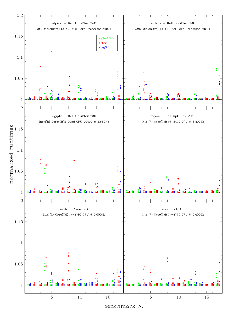
Figure 1: This panel shows, for six different individual PCs, the scatter in run-times after normalizing them to the best (minimum) value for each benchmark test and compiler. Green points refer to the gfortran compiler, red points to ifort, blue points to pgf90. The benchmark test N. 2 (aermod) fails when compiled with pgf90, and is thus omitted.

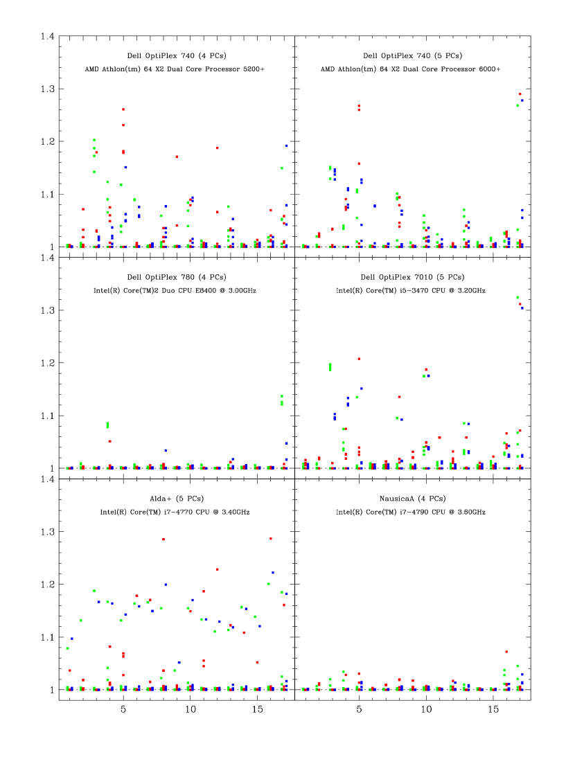
Figure 2: This panel shows, for six different PC models, the scatter in run-times after normalizing them to the best (minimum) value achieved for each model and benchmark test. The color scheme is the same as in Figure 1.

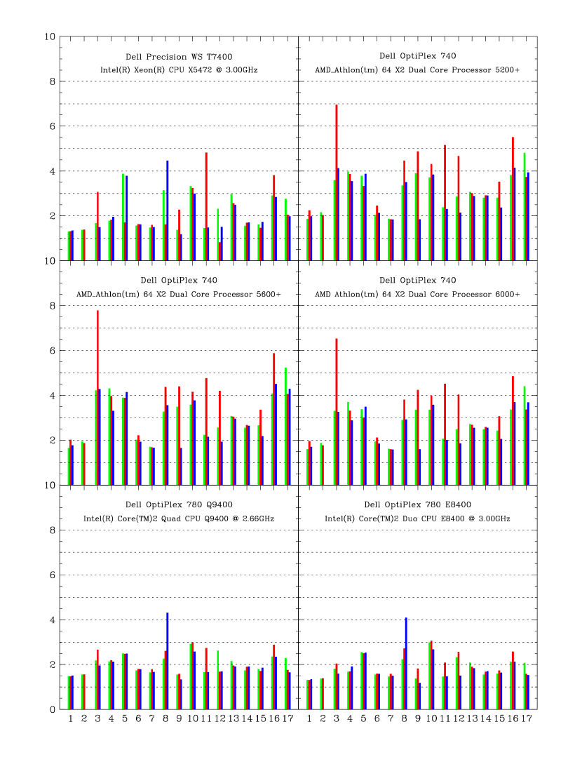
Figure 3: The best (minimum) run-times obtained in our tests for desktop and rack PCs are shown normalized to the value published by Polyhedron for a ”Sandy Bridge Intel Core i5 2500k” CPU. Again, green, red and blue indicates the gfortran, Intel Fortran and PGI Fortran compilers respectively.

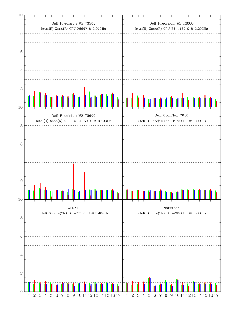
Figure 3: continued

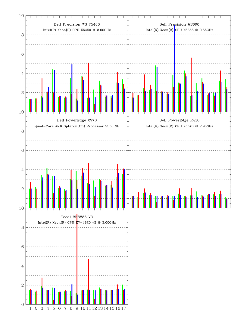
Figure 3: continued

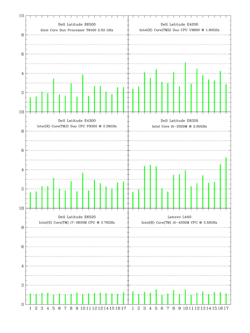
Figure 4: The best (minimum) run-times obtained in our tests for laptops are shown normalized to the value published by Polyhedron for a ”Sandy Bridge Intel Core i5 2500k” CPU. Due to license issues, only the gfortran tests were run on laptops.

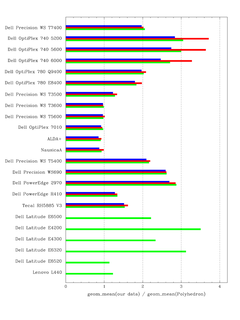
Figure 5: The geometrical mean of the execution times for the 17 benchmarks are shown normalized to the geometrical mean values published by Polyhedron for a Core i5 2500k 3.30GHz processor.

References

- MFL6VW [74649] http://www.polyhedron.com/MFL6VW74649
- [2] http://www.polyhedron.com/benchinstall
- [3] http://www.dell.com/support/home/us/en/19/Products/
- [4] http://research.cs.wisc.edu/htcondor/
- [5] Jim Basney, Miron Livny, and Todd Tannenbaum, ”High Throughput Computing with Condor”, HPCU news, Volume 1(2), June 1997.
- [6] Antonio Dorta, Nicola Caon, and Jorge A. Pérez Prieto, 2014, https://arxiv.org/abs/1412.5847
- [7] http://www.fortran.uk/historic-tables/polyhedron-fortran-benchmarks-64-bit-linux-on-intel-core-i5-2500k-december-2014/