Fast and unsupervised methods for multilingual cognate clustering

Abstract

In this paper we explore the use of unsupervised methods for detecting cognates in multilingual word lists. We use online EM to train sound segment similarity weights for computing similarity between two words. We tested our online systems on geographically spread sixteen different language groups of the world and show that the Online PMI system (Pointwise Mutual Information) outperforms a HMM based system and two linguistically motivated systems: LexStat and ALINE. Our results suggest that a PMI system trained in an online fashion can be used by historical linguists for fast and accurate identification of cognates in not so well-studied language families.

1 Introduction

Cognates are genetically related words that can be traced to a common word in a language that is no longer spoken. For example, English nail and German nagel are cognates with each other which can be traced back to the stage of Proto-Indo-European *$h_{3}enog^{h}-$. Accurate identification of cognates is important for inferring the internal structure of a language family.

Recent years has seen an surge in the number of publications in the field of computational historical linguistics due to the availability of word lists for large number of languages of the world (Brown et al., 2013) and cognate databases for Austronesian (Greenhill and Gray, 2009) and Indo-European (Bouckaert et al., 2012).

The availability of word lists (without cognate judgments) has allowed scholars like Rama and Borin (2015) and Jäger (2015) to experiment with different weighted string similarity measures for the purpose of inferring the family trees of world’s languages, without explicit cognate identification. On the other hand, List (2012) proposed a cognate clustering system that combines handcrafted weighted string similarity measures and permutation tests for the purpose of automated cognate identification. In a different approach, Hauer and Kondrak (2011) experimented with linear classifiers like SVMs for the purpose of identifying cognate clusters. Finally, Rama (2015) use string kernel inspired features for training a SVM linear classifier for pair-wise cognate identification. As noted by Hauer and Kondrak (2011), availability of a reliable multilingual cognate identification system can be used to supply the cognate judgments as an input to the phylogenetic inference algorithms introduced by Gray and Atkinson (2003) and reconstruction methods of Bouchard-Côté et al. (2013).

The phylogenetic inference methods require cognate judgments which are only available for a small number of well-studied language families such as Indo-European and Austronesian. For instance, the ASJP database provides Swadesh word lists (of length $40$ which are resistant to lexical replacement and borrowing) transcribed in a uniform format for more than $60\%$ of the world’s languages. However, the cognacy judgments are only available for a subset of language families. An example of such a word list is given in table 1.

	ALL	AND	ANIMAL	$\ldots$
English	ol	End	Enim3l	$\ldots$
German	al3	unt	tia	$\ldots$
French	tu	e	animal	$\ldots$
Spanish	to8o	i	animal	$\ldots$
Swedish	ala	ok	y3r	$\ldots$

Table 1: Example of a word list for five languages belonging to Germanic (English, German, and Swedish) and Romance (Spanish and French) subfamilies transcribed in ASJP alphabet.

The task at hand is to automatically cluster words that show genealogical relationship. This is achieved by computing similarities between all the word pairs belonging to a meaning and then supplying the resulting distance matrix as an input to a clustering algorithm. The clustering algorithm groups the words into clusters by optimizing a similarity criterion. The similarity between a word pair can be computed using supervised approaches (Hauer and Kondrak, 2011) or by using sequence alignment algorithms such as Needleman-Wunsch (Needleman and Wunsch, 1970) or Levenshtein distance (Levenshtein, 1966).

In dialectometry, Wieling et al. (2007) compared Pair Hidden Markov Model (PHMM) (Mackay and Kondrak, 2005) and pointwise mutual information (PMI) (Church and Hanks, 1990) weighted Levenshtein distance for Dutch dialect comparison. In historical linguistics, Jäger (2013) developed a PMI based method for computing the string similarity using the ASJP database. In this paper, we apply online algorithms to train our PMI and PHMM systems for the purpose of computing word similarity.

We train our PHMM and PMI systems in different settings and test it on sixteen different families of the world. Our results show that online training can perform better than a linguistically well-informed system known as LexStat (List, 2012). Also, the online algorithms allow our systems to be trained in few minutes and give similar accuracies as the batch trained systems of Jäger (2013).

The paper is organized as follows. We discuss the relevant work in section 2. We describe the PMI and PHMM models in section 3. The Online EM procedure is described in section 4. We describe the clustering algorithm in section 5. We discuss the experimental settings and motivation behind our choices in section 6. We present and discuss the results of our experiments in section 7. We discuss the effect of different model parameters in section 8. Finally, we conclude the paper in section 9.

2 Related work

Kondrak (2000) introduced a dynamic programming algorithm for computing the similarity between two sequences based on articulatory phonetic features determined by Ladefoged (1975). The author evaluated his algorithm on a list of English-Latin cognates. In this paper, we evaluate on the Indo-European dataset consisting of English and Latin.

Hauer and Kondrak (2011) trained a linear SVM on word similarity features and use the SVM model to assign a similarity score to the word pair. For each meaning, a word pair distance matrix is computed and supplied to the average linkage clustering algorithm for inferring cognate clusters. The authors observe that the SVM trained system performs better than a baseline that judges the similarity of two words based on the identity of the first two consonants.

List (2012) introduced a system known as LexStat (described in section 6) that is sensitive to segment similarities and chance similarities due to borrowing or semantic shift. The author tests this system on a number of small-sized (consisting of less than $20$ languages) datasets for the purpose of cognate identification and reports that the system performs better than Levenshtein distance.

In a recent paper, List et al. (2016) explore the use of InfoMap (Rosvall and Bergstrom, 2008) for the detection of partial cognates in subgroups of Sino-Tibetan language family. The authors compare the performance of average linkage clustering against InfoMap and find that InfoMap performs better than average linkage clustering.

The above listed works test similar datasets using different experimental settings. For instance, Hauer and Kondrak (2011) trained and tested on a subset of language families that were provided by Wichmann and Holman (2013). At the same time, to the best of our knowledge, the LexStat system has not been evaluated on all the available language families. Moreover, the PMI-LANG (Jäger, 2013), has not been evaluated at the task of unsupervised cognate clustering.

3 Models

In this section, we briefly describe the PMI weighted Needleman-Wunsch algorithm and Pair Hidden Markov Model (PHMM).

3.1 PMI-weighted alignment

The vanilla Needleman-Wunsch (VNW) algorithm is the similarity counterpart of the Levenshtein distance. It maximizes similarity whereas Levenshtein distance minimizes the distance. In VNW, a character or sound segment match increases the similarity by $1$ and a character mismatch has a weight of $-1$. In contrast to Levenshtein distance which treats insertion, deletion, and substitution equally, VNW introduces a gap opening (deletion operation) penalty parameter that has to be set separately. A second parameter known as gap extension penalty has lesser or equal penalty than the gap opening parameter and models the fact that deletions occur in chunks Jäger (2013).

VNW is not sensitive to segment pairs, but a realistic algorithm should assign higher similarity score to sound correspondences such as /l/ $\sim$ /r/ than the sound correspondences /p/ $\sim$ /r/. The weighted Needleman-Wunsch algorithm requires a similarity score for each pair of segments, and it finds the alignment(s) betwen two input strings maximizing the sum of the pairwise similiarities of matched segment pairs.

In computational historical linguistics, similarity between two segments is estimated using PMI. The PMI score for two sounds $i$ and $j$ is defined as followed:

$$\textnormal{PMI}(i,j)=\log\frac{p(i,j)}{q(i)\cdot q(j)}$$ (1)

where, $p(i,j)$ is the probability of $i,j$ being matched in a pair of cognate words, whereas, $q(i)$ is the probability that an arbitrarily chosen segment in an arbitrarily chosen word equals $i$. A positive PMI value between $i$ and $j$ indicates that the probability of $i$ being aligned with $j$ in a pair of cognates is higher than what would be expected by chance. Conversely, a negative PMI value indicates that an alignment of $i$ with $j$ is more likely the result of chance than of shared inheritance.

We estimated PMI scores from raw data, largely following the method described in Jäger (2013).

The whole training procedure can be described as follows:

1. Extract a set of word pairs that are probably cognate using a suitable heuristics. In this paper, we treat all word pairs belonging to the same meaning with a length normalized Levenshtein distance (LDN) below $0.5$ as probable cognates.

2. Align the list of probable cognates using the vanilla Needleman-Wunsch algorithm.

3. Extract aligned segment pairs and compute the PMI value for a segment pair using equation 1 and estimating probabilities as relative frequencies.

4. Generate a new set of aligments using Needleman-Wunsch algorithm and the segment weights learned from step 2. For the gap penalties we used the values proposed in Jäger (2013).

5. We iterate between step 2 and 3 until the average similarity between the two iterations does not change.

This procedure yields a PMI based similarity score for each word pair. We convert the similarity score $x$ into a distance score using the sigmoid transformation: $1.0-(1+exp(-x))^{-1}$ that converts the PMI similarity score into the range of $[0,1]$.

3.2 Pair Hidden Markov Model

Pair Hidden Markov Model was first proposed in the context of computational biology as a tool for the comparison of DNA or protein sequences (Durbin et al., 2001).

A Pair Hidden Markov Model (PHMM) uses two output streams, instead of a single output stream; one for each of the two sequences being aligned. In its simplest version, a PHMM consists of five states. A begin state, an end state, a match state (M) that emits pairs of symbols, a deletion state (X) that emits a symbol in the first string and a gap in the second string; and an insertion state (Y) that emits a gap in the first and a symbol in the second string (cf. figure 1).

Figure 1: Pair Hidden Markov model as proposed by Mackay & Kondrak (Mackay and Kondrak, 2005). The states of the model are depicted as the circles. The arrows show the possible transitions between the states. $<\delta,\epsilon,\lambda,\tau_{M},\tau_{XY}>$ represent the transition probabilities.

The PHMMs, as used in historical linguistics, differ from its biological counterpart in the following regard:

• The historical linguistic PHMM allows a transition between the states X and Y (dashed line, figure 1). An alignment of Italian due and Spanish dos ‘two’ cannot be generated by a PHMM without the transition between X and Y (Mackay and Kondrak, 2005).

  d u e -

  d o - s

• Another difference between the biological and the linguistic PHMM is the split of the parameter for the transition into the end state. Whilst the original version only has one parameter for this purpose, the linguistic PHMM makes use of two different probabilities $\tau_{M}$ and $\tau_{XY}$. This split of parameters enables the model to distinguish between the match state (M) being the final emitting state or any of the gap states (X,Y) (see figure 1). This modification preserves the symmetry of the model, while allowing a little bit more freedom.

The PHMMs are trained using Baum-Welch expectation maximization algorithm (Durbin et al., 2001). The best alignment between two sequences $x$ and $y$ is determined by using the Viterbi algorithm.

The probability of two sequences $x$ and $y$ of lengths $m$ and $n$ respectively evolving independently under a null model $R$ is given by the following equation 2.

$$P(x,y|R)=\iota^{2}(1-\iota)^{n+m}\prod\limits_{i=1}^{n}f_{x_{i}}\prod\limits_{j=1}^{m}f_{y_{j}},$$ (2)

with $f_{x_{i}}$ is the equilibrium frequency of the sound at position $i$ in sequence $x$ where, $\iota=\frac{1}{\frac{m+n}{2}+1}.$

The probability of relatedness between $x$ and $y$ is computed as the logarithmic ratio of the probability scores $P(x,y|\mu)$ and $P(x,y|R)$, where $\mu$ is the trained model and $R$ is the null model.

We employ the same sigmoid transformation, as in PMI, to convert the similarity score (computed under a PHMM) to a distance score.

4 Online EM

The Expectation Maximization algorithm (EM) is widely used in computational linguistics for the purpose of word alignment, document classification, and word segmentation. The EM algorithm starts with an initial setting of model parameters and uses that model parameters to realign words in a sentence pair. The model parameters are reestimated using the word alignments obtained from the previous iteration. The EM algorithm reestimates the model parameters after each full scan of the training data.

Liang and Klein (2009) observe that batch training procedure can lead to slow convergence. As a matter of fact, Jäger (2013) trains his PMI system using the standard EM (also known as batch EM) which updates the parameters in a PMI scoring matrix only after aligning all the word pairs. In contrast, Online EM (Liang and Klein, 2009), updates the model parameters after aligning a subset of word pairs (also known as minibatch in online learning literature).

The Online EM algorithm combines the parameters estimated ($s$) from the current update step $k$ with the previous parameters $\theta_{k-1}$ using the following equation:

$$\theta_{k}=(1-\eta_{k})\theta_{k-1}+\eta_{k}s$$ (3)

where $\eta_{k}$ is defined as: $\eta_{k}=(k+2)^{-\alpha}$.

In the case of PMI, $\theta$ constitutes the PMI scores for all segment pairs. The parameter $\eta_{k}$ determines how fast to forget or remember the updates from the previous steps. The $\alpha$ parameter is in the range of $0.5\leq\alpha\leq 1$. A smaller $\alpha$ implies a large update to the model parameters. The parameter $k$ is related to minibatch parameter ($m$; $m=\lceil D/k\rceil$; where, $D$ is the size of training data) and determines the number of updates to be performed. The setting $k=1$ recovers the batch EM whereas, when $k=D$, implies an update for each sample in the training data.

5 Clustering algorithm

The InfoMap clustering method is an information theoretic approach to detect community structure within a connected network. The method uses random walks on a network as a proxy for information flow to detect communities, i.e., clusters, without the need for a threshold. A community is a group of nodes with more edges connecting the nodes within the community than connecting them with nodes outside the community (Newman and Girvan, 2004).

In our case, a community refers to the words which are cognate and have higher edge weights between them. The idea behind the algorithm is that the random walk is statistically more likely to spend a long period of time within a community than switching communities due to the nature of the network.

A pair-wise distance matrix is a complete weighted graph and any edge that has a weight $<0.5$ and a PMI score $<0$ (due to the sigmoid-based distance transformation). Due to the PMI score’s definition, a PMI score $<0$ implies that the words might not be cognate. We use this property to construct a non-complete graph and supply the resulting network as an input to the InfoMap algorithm.

6 Experiments

In this section, we describe the experimental settings, datasets, evaluation measures, and the comparing systems: Baseline, ALINE, PMI-LANG, and LexStat.

6.1 Hyperparameters of Online EM

We determine the best setting of $m$ and $\alpha$ parameter by searching for $m$ in the range of $m=2^{s}$ where $s\in[5,15]$; and, $\alpha\in[0.5,1.0]$ with a step size of $0.05$. We fix the gap opening and gap extension penalties to $-2.5$ and $-1.75$.

6.2 Datasets

6.2.1 Indo-European database

The Indo-European Lexical database (IELex) was created by Dyen et al. (1992) and curated by Michael Dunn. The IELex database is not transcribed in uniform IPA and retains many forms transcribed in the Romanized IPA format of Dyen et al. (1992). We cleaned the IELex database of any non-IPA-like transcriptions and converted the cleaned subset of the database into ASJP format.

6.2.2 Austronesian vocabulary database

The Austronesian Vocabulary Database (ABVD) (Greenhill and Gray, 2009) has word lists for $210$ Swadesh concepts and $378$ languages. The database does not have transcriptions in a uniform IPA format. We removed all symbols that do not appear in the standard IPA and converted the lexical items to ASJP format. For comparison purpose, we use randomly selected $100$ languages’ dataset in this paper.

6.2.3 Short word lists with cognacy judgments:

Wichmann and Holman (2013) and List (2014a) compiled cognacy wordlists for subsets of families from various scholarly sources such as comparative handbooks and historical linguistics’ articles. The details of different databases is given in table 2.

Family	NOM	NOL	AveCC	AveWC
Austronesian	210	100	20.2142	4.1143
Afrasian	40	21	9.5	2.6868
Bai dialects	110	9	2.5909	6.0166
Chinese dialects	179	18	6.8771	5.2635
Huon	84	14	6.3929	2.7672
Indo-European	207	52	12.2126	7.3461
Japanese dialects	200	10	2.3	6.1373
Kadai	40	12	3.225	5.0027
Kamasau	36	8	1.6667	5.3981
Lolo-Burmese	40	15	2.625	7.3121
Mayan	100	30	8.58	6.1521
Miao-Yao	39	6	1.8974	3.9667
Mixe-Zoque	100	10	3	4.6535
Mon-Khmer	100	16	7.75	2.7956
ObUgrian	110	21	2.2	11.8162
Tujia	109	5	1.6422	3.3792

Table 2: Number of languages (NOL), Number of meanings (NOM), Average number of cognate classes per meaning (AveCC), and Average number of words per cognate class (AveWC).

6.3 Evaluation Measures

We evaluate the results of clustering analysis using B-cubed F-score (Amigó et al., 2009). The B-cubed scores are defined for each word belonging to a meaning as followed. The precision for a word is defined as the ratio between the number of cognates in its cluster to the total number of words in its cluster. The recall for a word is defined as the ratio between the number of cognates in its cluster to the total number of expert labeled cognates. The B-cubed precision and recall are defined as the average of the words’ precision and recall across all the clusters. Finally, the B-cubed F-score for a meaning, is computed as the harmonic mean of the average items’ precision and recall. The Averaged B-cubed F-score for the whole dataset is computed as the average of the B-cubed F-scores across all the meanings.

Amigó et al. (2009) show that the B-cubed F-score satisfies four formal constraints known as cluster homogeneity, cluster completeness, rag bag (robustness to misplacement of a true singleton item), and robustness to variation in cluster size. The authors show that cluster evaluation measures based on entropy such as Mutual Information and V-measure (Rosenberg and Hirschberg, 2007) and Rand index do not satisfy the four constraints. Both Hauer and Kondrak (2011) and List et al. (2016) use B-cubed F-scores to evaluate their cognate clustering systems.

6.4 Comparing systems

Baseline We adopt length normalized Levenshtein distance as the baseline in our experiments.

6.4.1 ALINE

ALINE is a sequence alignment system designed by Kondrak (2000) for computing similarity between two words by decomposing phonemes into multivalued and binary phonetic features. Each phoneme is decomposed into multivalued features such as place and manner for consonants; height and backness for vowels. Multivalued features take values on a continous scale ranging from $[0,1]$ and the values represent the distance between the sources of articulation. Binary valued features consist of nasal, voicing, aspirated, and retroflex.

Each feature is weighed by a salience value that is determined manually. The similarity score between two sequences is computed as the sum of the aligned sound segments. Following Downey et al. (2008), we convert ALINE’s similarity score $s_{ab}$ between two words $a,b$ is converted to a distance score based on the following formula: $1.0-\frac{2.0*s_{ab}}{s_{aa}+s_{bb}}$.

6.4.2 PMI-LANG

Jäger (2013) developed a system that learns PMI sound matrices to optimize a criterion designed to optimize language relatedness. The core idea is to tie up word similarity to language similarity such that close languages such as English/German tend to have more similarity than English/Hindi. The language similarity function amounts to maximizing similarity between probable cognates to learn a PMI score matrix. Jäger (2013) applies the learned PMI score matrix to infer phylogenetic trees of language families. However, the learned PMI score matrix has not been applied for cognate clustering.

6.4.3 LexStat

LexStat (List, 2012) is part of LingPy (List and Forkel, 2016) library offering state-of-the-art alignment algorithms for aligning word pairs and clustering them into cognate sets. We describe the workflow of LexStat system below:

1. LexStat uses a hand-crafted sound segment matrix, $h$, to align and score the word pairs for each meaning. Let a segment pair $i,j$’s similarity be given as $h_{ij}$.

2. For each language pair, $l_{1},l_{2}$ the word pairs belonging to the same meaning are aligned. The frequency of a segment pair $i,j$ belonging to the same meaning is given as $a_{ij}$.

3. For $l_{1},l_{2}$, the words belonging to one of the language is shuffled and realigned using Needleman-Wunsch algorithm. This procedure is repeated for all language pairs for $100$ times. The average frequency of a segment pair $i,j$ from the reshuffling step is given as $e_{ij}$.

4. All the parameters $h,a,e$ are combined according to the following formula to give a new segment similarity score $s_{ij}$ where, $w_{1}+w_{2}=1$.

   $$s_{ij}=2*w_{1}log\frac{a_{ij}}{e_{ij}}+w_{2}h_{ij}$$ (4)

5. The weights $s_{ij}$ are then used to score word pairs and cluster words in a meaning.

The intuition behind step 3 is to reduce the effect of chance similarities between the sound segments that can obscure real genetic sound correspondences. We supply the word distances from all the above systems as input to InfoMap to infer cognate clusters.

7 Results

In this section, we present the results of our experiments. We perform two sets of experiments by training with different datasets which are described below.

Family	LDN	PMI-LANG	Batch PMI	Online PMI	Batch PHMM	Online PHMM	LexStat	ALINE
Austronesian	0.7175	0.7355	0.6539	0.7364	0.6224	0.6709	0.7173	0.5321
Afrasian	0.7993	0.8133	0.7496	0.8392	0.7213	0.7044	–	0.6442
Bai dialects	0.8348	0.8766	0.8716	0.8774	0.8741	0.8639	0.8417	0.8462
Chinese dialects	0.7687	0.7521	0.7217	0.7803	0.7455	0.7396	0.7815	0.6651
Huon	0.8536	0.8556	0.7518	0.8775	0.7612	0.7437	–	0.6413
Indo-European	0.7367	0.7752	0.7337	0.7812	0.715	0.7126	0.7316	0.6583
Japanese dialects	0.893	0.9031	0.8943	0.9051	0.9006	0.9083	0.8875	0.8699
Kadai	0.7581	0.8175	0.8139	0.8309	0.8	0.8159	–	0.7647
Kamasau	0.9561	0.9850	0.9543	0.9823	0.9605	0.9674	–	0.9479
Lolo-Burmese	0.6469	0.713	0.7862	0.7805	0.7846	0.8218	–	0.8027
Mayan	0.8198	0.7798	0.6958	0.8074	0.6804	0.6797	0.7931	0.627
Miao-Yao	0.6412	0.7003	0.7679	0.7801	0.7411	0.7879	–	0.8426
Mixe-Zoque	0.9055	0.9149	0.8528	0.9209	0.8521	0.8599	0.8656	0.8298
Mon-Khmer	0.7883	0.8209	0.7054	0.8302	0.6921	0.7008	0.7925	0.6472
ObUgrian	0.8623	0.911	0.8987	0.9214	0.8951	0.8874	0.8837	0.8826
Tujia	0.8882	0.9091	0.9018	0.9105	0.895	0.9027	0.8905	0.8757
Average	0.8044	0.8289	0.7971	0.8415	0.7901	0.7955	0.8185	0.7548

Table 3: The B-cubed F-scores of different models on sixteen language groups. The last row reports the average of the B-cubed F-scores across all the datasets. The numbers in bold show the highest scores across columns.

7.1 Out-of-family training

In this experiment, we train our PHMM and PMI systems on wordlists from the ASJP database belonging to families other than those language groups present in table 2. We made sure that there is no overlap between the languages present in test dataset and the training dataset. We extracted a list of probable cognates and trained our PMI and PHMM models on the list of probable cognates. We trained all the batch and online systems on $1151178$ word pairs. The results of our experiments are given in table 3. We report the InfoMap clustering results for a threshold of $0.5$ for all the systems. We expect LexStat to perform better in the case of Chinese since LexStat handles tones internally whereas, the ASJP representation does not handle tones. In the case of online systems, we report the best results for $m,\alpha$. Following List (2014b), we do not report LexStat results for the language groups which have word lists shorter than $100$ meanings.

	PMI		PHMM
Family	$m$	$\alpha$	$m$	$\alpha$
Austronesian	64	0.75	32	0.5
Afrasian	256	0.65	32	0.8
Bai dialects	8192	0.75	32	0.55
Chinese dialects	128	0.95	512	0.6
Huon	32	1	32	0.65
Indo-European	512	0.55	1024	0.5
Japanese dialects	512	0.55	32	0.6
Kadai	2048	0.7	32	0.7
Kamasau	512	0.5	128	0.55
Lolo-Burmese	16384	0.5	32	0.75
Mayan	64	0.5	32	0.55
Miao-Yao	8192	0.95	128	0.7
Mixe-Zoque	256	0.7	32	0.7
Mon-Khmer	256	0.7	32	0.5
ObUgrian	512	0.75	32768	0.5
Tujia	1024	0.65	32	0.5

Table 4: Best settings of $m$ and $\alpha$ for Online variants of PMI and PHMM.

The Online PMI performs better than the rest of the systems at nine out of the sixteen families. On an average, the Online PMI system ranks the best followed by PMI-LANG and LexStat system. ALINE performs the best on Miao-Yao language group. The Online PMI system perform better than the Batch PMI on all the datasets. As expected, the LexStat system performs the best on Chinese dialect dataset. Surprisingly, despite its complexity the PHMM systems do not perform as well as the simpler PMI systems.

Now, we will comment on the results of Austronesian and Indo-European language families. Greenhill (2011) applied Levenshtein distance for the classification of Austronesian languages and argued that Levenshtein distance does not perform well at the task of detecting language relationships. Our experiment shows that Levenshtein distance comes close to LexStat in the case of Austronesian language family. Both PMI-LANG and Online PMI are two points better than Levenshtein distance at the task of cognate identification.

The results are much clearer in the case of Indo-European language family. The PMI-LANG and Online PMI systems perform better than rest of the systems. Levenshtein distance performs better than LexStat for the Indo-European language family. On an average, ALINE shows the lowest performance of all the systems.

We report the corresponding setting of $m,\alpha$ for all the online systems in table 4. The value of $m$ is quite variable across language families whereas, $\alpha$ tends to be in the range of $0.5-0.75$. We investigate the effect of $m$ and $\alpha$ for Indo-European and Austronesian languages by plotting the results of Online PMI system in figures 2. The B-cubed F-scores are stable across the range of $\alpha$ but show variable results for value of $m$. The top-3 F-scores for Indo-European are at $m=256,512,1024$ and at $m=64,128,256$ for Austronesian language family. These results suggest that the online training helps cognate clustering than the batch training. The plots (cf. figure 2) suggest that small batch size improves the performance whereas a large batch size (eg., 32768) hurts the performance on Indo-European and Austronesian language families.

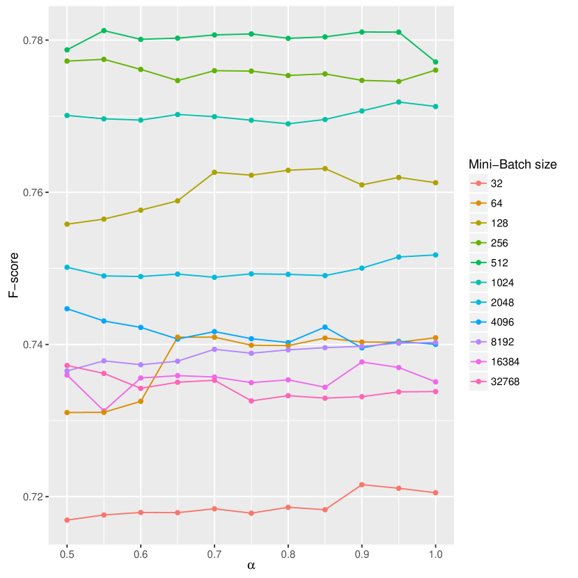
(a) Indo-European

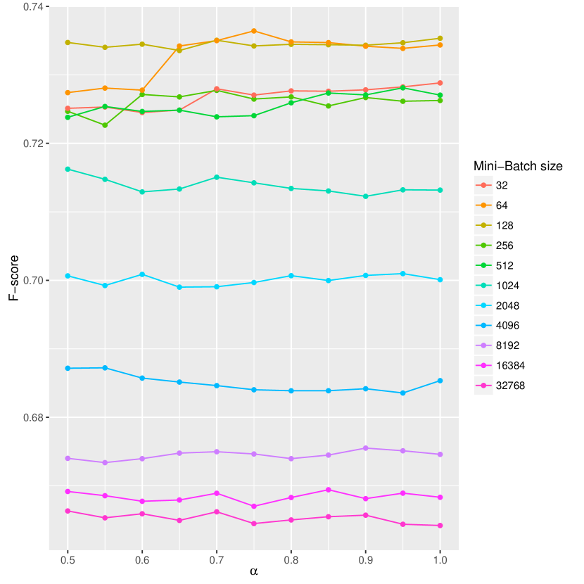
(b) Austronesian

Figure 2: Plots of $m$ and $\alpha$ against B-cubed F-scores for out-of-family training.

7.2 Within-family training

Family	Training word pairs	Online PHMM			Online PMI			Batch PHMM	Batch PMI
		$m$	$\alpha$	F-score	$m$	$\alpha$	F-score
ASJP Indo-European	380769	128	0.60	0.7646	4096	0.60	0.7868	0.7656	0.7704
Indo-European	25386	64	0.50	0.7901	1024	0.85	0.7971	0.7797	0.7914
ASJP Mayan	91665	256	0.55	0.7765	128	0.90	0.8250	0.7814	0.7677
Mayan	11889	32	0.55	0.7952	64	0.70	0.7997	0.7888	0.7544
ASJP Austronesian	1000000	32	0.65	0.6190	128	0.80	0.7453	0.6239	0.6429
Austronesian	84311	32	0.5	0.6709	128	0.80	0.7460	0.6517	0.6509

Table 5: The results of training the PMI and PHMM systems on the ASJP 40 word lists and the full word lists of Indo-European, Mayan, and Austronesian.

In this experiment, we train our PMI and PHMM systems on three largest language families in our dataset: Mayan, Indo-European, and Austronesian language families. We train our systems on word pairs extracted from two different sources.

1. The ASJP database has $40$-length word lists for more languages ($\sim$ 3 times) than the languages in cognate databases of Mayan, Indo-European, and Austronesian language families. The database allows us to access more word pairs than any other database in existence.

2. We extract list of probable cognate pairs from the IELex, ABVD, and Mayan language databases.

The motivation behind these experiments is to investigate the performance of PMI and PHMM systems when trained on the word lists belonging to the same language family but compiled by different group of annotators. A successful experiment indicates that this approach of training a PMI matrix on ASJP $40$ word lists can be applied to language families that have longer word lists but no cognate judgments. The number of training word pairs and the results of our experiments are given in table 5.

The Online variants perform better than the batch systems across all the language families and settings. Online PMI performs the best across all the language families than the Batch PMI. Online PMI trained on ASJP word lists of a language family show close performance to an Online PMI system trained within the language family in the case of Indo-European and Austronesian language families. The performance of batch PMI system comes close to the Online PMI system in the case of Indo-European but falls behind in the case of other language families. Training the online system on ASJP word lists improves the performance in the case of Mayan language family. This performance is not observed in the case of Indo-European and Austronesian language families. The reason for this could be due to the source of origin of the datasets.

The batch PMI/PHMM systems perform better than LexStat on Indo-European and Mayan language families. The Online PHMM system comes close in performance to Online PMI system in the case of Indo-European and Mayan language families. PHMM systems how the lowest performance on Austronesian language family. Except for Indo-European, the best batch sizes for online PMI system are small and are typically $\leq 256$.

8 Discussion

In this section, we discuss the effects of various parameters on our results.

8.1 Effect of $m$ and $\alpha$

Throughout our experiments, we observe that low minibatch size gives better results than a large minibatch size. We also observe that a intermediary value of $\alpha$ is usually sufficient for obtaining the best results.

Figure 2 shows that small values of $m$ yields stable F-scores across the range of $\alpha$. Small values of $m$ typically gives better results than larger values of $\alpha$. In contrast to other NLP tasks that require large $m$ and smaller $\alpha$, the task of aligning two words requires smaller values of $m$. The small value of $m$ implies large number of updates which is important for a task where the average sequence length ($\sim 5$) and the average number of word pairs are in less than $100,000$. Further, an intermediary value of $\alpha$ controls the amount of memory retained at each update.

8.2 Speed

One advantage of our online systems (either PMI or PHMM) is that the training time is typically in the range of $10$ minutes on a single thread of i7-6700 processor. In the case of PHMM, online training speeds up the convergence and yields, typically, better results than the batch variant. In comparison, the PMI-LANG system takes days to train. Finally, our results show that the online algorithm can yield better performance than LexStat. LexStat and PHMM take more than 5 hours to test on the language subset of the Austronesian language family. In contrast, PMI (both online and batch) takes less than $10$ minutes for each value of $m,\alpha$ in the case of out-of-family training. We also observe that $5$ scans over the full data was sufficient for convergence.

8.3 Analyzing PHMM’s performance

Although PHMMs are the most complex among the tested models, the performance of these models is not as good as the conceptually simpler PMI models. This lack of performance could be due to the characteristics of the PHMM. The transition probability from the begin state to the match or gap states is the same as the transition probability from the match state to either gap state or itself (figure 1). Although desirable for biological purposes, this poses a big problem for linguistic applications. To start an alignment with a match is more likely than to start with a gap.

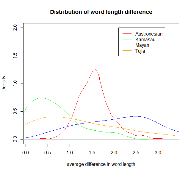
Figure 3: Distribution of average of word length differences across concepts.

Therefore, the alignments generated by PHHMs are more likely to show gaps at the end of the string than in the beginning. This results in problems for data sets where word length differ a lot. The PHMM performs the worst for those datasets that show a huge difference in the word length. On the other hand, for Kamasau and Tujia – the two datasets with the best performance – the difference in word length is much less pronounced (cf. figure 3).

Based on the results of these experiments, we propose that training the PMI-based segment scores in an online fashion and supplied to InfoMap clustering could yield reliable cognate judgments.

9 Conclusion

In this paper, we evaluated the performance of various sequence alignment algorithms – both learned and linguistically designed – for the task of cognate detection across different language families. We find that training PMI and PHMM in an online fashion speeds up convergence and yields comparable or better results than the batch variant and the state-of-the-art LexStat system. Online PMI system shows the best performance across different language families. In conclusion, PMI systems can be trained faster in an online fashion and yield better accuracies than the current state-of-the-art systems.

References

- Amigó et al. [2009] Enrique Amigó, Julio Gonzalo, Javier Artiles, and Felisa Verdejo. A comparison of extrinsic clustering evaluation metrics based on formal constraints. Information retrieval, 12(4):461–486, 2009.
- Bouchard-Côté et al. [2013] Alexandre Bouchard-Côté, David Hall, Thomas L. Griffiths, and Dan Klein. Automated reconstruction of ancient languages using probabilistic models of sound change. Proceedings of the National Academy of Sciences, 110(11):4224–4229, 2013. doi: 10.1073/pnas.1204678110. URL http://www.pnas.org/content/early/2013/02/05/1204678110.abstract.
- Bouckaert et al. [2012] Remco Bouckaert, Philippe Lemey, Michael Dunn, Simon J. Greenhill, Alexander V. Alekseyenko, Alexei J. Drummond, Russell D. Gray, Marc A. Suchard, and Quentin D. Atkinson. Mapping the origins and expansion of the Indo-European language family. Science, 337(6097):957–960, 2012.
- Brown et al. [2013] Cecil H. Brown, Eric W. Holman, and Søren Wichmann. Sound correspondences in the world’s languages. Language, 89(1):4–29, 2013.
- Church and Hanks [1990] Kenneth Ward Church and Patrick Hanks. Word association norms, mutual information, and lexicography. Computational Linguistics, 16(1):22–29, 1990. ISSN 0891-2017.
- Downey et al. [2008] Sean S Downey, Brian Hallmark, Murray P Cox, Peter Norquest, and J Stephen Lansing. Computational feature-sensitive reconstruction of language relationships: Developing the aline distance for comparative historical linguistic reconstruction. Journal of Quantitative Linguistics, 15(4):340–369, 2008.
- Durbin et al. [2001] Richard Durbin, Sean R Eddy, Anders Krogh, and Graeme Mitchison. Biological sequence analysis: probabilistic models of proteins and nucleic acids. Cambridge Univ. Press, repr. edition, 2001.
- Dyen et al. [1992] Isidore Dyen, Joseph B. Kruskal, and Paul Black. An Indo-European classification: A lexicostatistical experiment. Transactions of the American Philosophical Society, 82(5):1–132, 1992.
- Gray and Atkinson [2003] Russell D Gray and Quentin D Atkinson. Language-tree divergence times support the anatolian theory of indo-european origin. Nature, 426(6965):435–439, 2003.
- Greenhill [2011] Simon J Greenhill. Levenshtein distances fail to identify language relationships accurately. Computational Linguistics, 37(4):689–698, 2011.
- Greenhill and Gray [2009] Simon J. Greenhill and Russell D. Gray. Austronesian language phylogenies: Myths and misconceptions about Bayesian computational methods. Austronesian Historical Linguistics and Culture History: A Festschrift for Robert Blust, pages 375–397, 2009.
- Hauer and Kondrak [2011] Bradley Hauer and Grzegorz Kondrak. Clustering semantically equivalent words into cognate sets in multilingual lists. In Proceedings of the 5th International Joint Conference on Natural Language Processing, pages 865–873, 2011.
- Huff and Lonsdale [2011] Paul Huff and Deryle Lonsdale. Positing language relationships using aline. Language Dynamics and Change, 1(1):128–162, 2011.
- Jäger [2013] Gerhard Jäger. Phylogenetic inference from word lists using weighted alignment with empirically determined weights. Language Dynamics and Change, 3(2):245–291, 2013.
- Jäger [2015] Gerhard Jäger. Support for linguistic macrofamilies from weighted sequence alignment. Proceedings of the National Academy of Sciences, 112(41):12752–12757, 2015. doi: –10.1073/pnas.1500331112˝.
- Kondrak [2000] Grzegorz Kondrak. A new algorithm for the alignment of phonetic sequences. In Proceedings of the 1st North American chapter of the Association for Computational Linguistics conference, pages 288–295. Association for Computational Linguistics, 2000.
- Ladefoged [1975] Peter Ladefoged. A course in phonetics. Hardcourt Brace Jovanovich Inc. NY, 1975.
- Levenshtein [1966] V. I. Levenshtein. Binary codes capable of correcting deletions, insertions, and reversals. Soviet Physics Doklady, 10(8):707–710, 1966.
- Liang and Klein [2009] Percy Liang and Dan Klein. Online em for unsupervised models. In Proceedings of Human Language Technologies: The 2009 Annual Conference of the North American Chapter of the Association for Computational Linguistics, NAACL ’09, pages 611–619, Stroudsburg, PA, USA, 2009. Association for Computational Linguistics. ISBN 978-1-932432-41-1. URL http://dl.acm.org/citation.cfm?id=1620754.1620843.
- List [2012] Johann-Mattis List. Lexstat: Automatic detection of cognates in multilingual wordlists. In Proceedings of the EACL 2012 Joint Workshop of LINGVIS & UNCLH, pages 117–125. Association for Computational Linguistics, 2012.
- List [2014a] Johann-Mattis List. Sequence comparison in historical linguistics. Düsseldorf University Press, Düsseldorf, 2014a. URL http://sequencecomparison.github.io/.
- List [2014b] Johann-Mattis List. Investigating the impact of sample size on cognate detection. Journal of Language Relationship, 11:91–101, 2014b.
- List and Forkel [2016] Johann-Mattis List and Robert Forkel. Lingpy. a python library for historical linguistics, 2016. URL http://lingpy.org.
- List et al. [2016] Johann-Mattis List, Philippe Lopez, and Eric Bapteste. Using sequence similarity networks to identify partial cognates in multilingual wordlists. In Proceedings of the 54th Annual Meeting of the Association for Computational Linguistics (Volume 2: Short Papers), pages 599–605, Berlin, Germany, August 2016. Association for Computational Linguistics. URL http://anthology.aclweb.org/P16-2097.
- Mackay and Kondrak [2005] Wesley Mackay and Grzegorz Kondrak. Computing word similarity and identifying cognates with pair hidden Markov models. CONLL ’05, pages 40–47, Stroudsburg, PA, USA, June 2005. Association for Computational Linguistics.
- Needleman and Wunsch [1970] Saul B. Needleman and Christian D. Wunsch. A general method applicable to the search for similarities in the amino acid sequence of two proteins. Journal of Molecular Biology, 48(3):10, 1970.
- Newman and Girvan [2004] Mark EJ Newman and Michelle Girvan. Finding and evaluating community structure in networks. Phys. Rev. E, 69:026113, Feb 2004. doi: 10.1103/PhysRevE.69.026113. URL http://link.aps.org/doi/10.1103/PhysRevE.69.026113.
- Rama [2015] Taraka Rama. Automatic cognate identification with gap-weighted string subsequences. In Proceedings of the 2015 Conference of the North American Chapter of the Association for Computational Linguistics: Human Language Technologies., pages 1227–1231, 2015.
- Rama and Borin [2015] Taraka Rama and Lars Borin. Comparative evaluation of string similarity measures for automatic language classification. In Ján Mačutek and George K. Mikros, editors, Sequences in Language and Text, pages 203–231. Walter de Gruyter, 2015.
- Rosenberg and Hirschberg [2007] Andrew Rosenberg and Julia Hirschberg. V-measure: A conditional entropy-based external cluster evaluation measure. In EMNLP-CoNLL, volume 7, pages 410–420, 2007.
- Rosvall and Bergstrom [2008] Martin Rosvall and Carl T. Bergstrom. Maps of random walks on complex networks reveal community structure. Proceedings of the National Academy of Sciences, 105(4):1118–1123, 2008. doi: 10.1073/pnas.0706851105. URL http://www.pnas.org/content/105/4/1118.abstract.