Performance Analysis of Dense Small Cell Networks with Generalized Fading

Abstract

In this paper, we propose a unified framework to analyze the performance of dense small cell networks (SCNs) in terms of the coverage probability and the area spectral efficiency (ASE). In our analysis, we consider a practical path loss model that accounts for both non-line-of-sight (NLOS) and line-of-sight (LOS) transmissions. Furthermore, we adopt a generalized fading model, in which Rayleigh fading, Rician fading and Nakagami-$m$ fading can be treated in a unified framework. The analytical results of the coverage probability and the ASE are derived, using a generalized stochastic geometry analysis. Different from existing work that does not differentiate NLOS and LOS transmissions, our results show that NLOS and LOS transmissions have a significant impact on the coverage probability and the ASE performance, particularly when the SCNs grow dense. Furthermore, our results establish for the first time that the performance of the SCNs can be divided into four regimes, according to the intensity (aka density) of BSs, where in each regime the performance is dominated by different factors.

I Introduction

With increasing demands on wireless data driven by smartphones, tablets, and video streaming, wireless data traffic is expected to overwhelm cellular networks in the near future. Against this background, network densification, together with millimeter wave and massive multiple-input multiple-output, have been envisioned to be “the three pillars” to support the vision of the emerging fifth generation (5G) wireless networks in the future to accommodate the phenomenal growth of wireless data traffic [1]. In this context, the orthogonal deployment of dense small cellular networks (SCNs) [2, 3] has been selected as the workhorse for capacity enhancement in the fourth generation (4G) and the 5G networks developed by the third Generation Partnership Project (3GPP). In this paper, we focus on the analysis of such dense SCNs.

Different from most previous work studying network performance where the propagation path loss between the base staions (BSs) and the mobile users (MUs) follows the same power-law model, in this paper we consider the co-existence of both non-line-of-sight (NLOS) and line-of-sight (LOS) transmissions, which frequently occur in urban areas. More specifically, for a randomly selected MU, BSs deployed according to a homogeneous Poisson point process (PPP) are divided into two categories, i.e., NLOS BSs and LOS BSs, depending on the distance between the BSs and the MU. In this context, the authors of [4] studied the coverage and capacity performance by using a multi-slop path loss model incorporating probabilistic NLOS and LOS transmissions. The authors of [5] and [6] analyzed the coverage and capacity performance in millimeter wave cellular networks. In [5], a three-state statistical model for each link was assumed, in which a link can either be in a NLOS, LOS or in an outage state. In [6], self-backhauled millimeter wave cellular networks were characterized assuming a cell association scheme based on the smallest path loss. However, both [5] and [6] assumed a noise-limited network, ignoring inter-cell interference, which may not be very practical since modern wireless networks generally work in an interference-limited region.

In this work, we will study the performance impact on the coverage probability and the ASE caused by the coexistence of both NLOS and LOS transmissions in dense SCNs with a generalized fading model. Furthermore, the proposed framework can also be applied to analyze dense SCNs, where BSs are distributed according to non-homogeneous PPPs, i.e., the BS intensity (aka density) varies in the spatial domain. The main contributions of this paper are as follows:

• A general SCN model: For characterizing the signal-to-interference-plus-noise ratio (SINR) coverage probabiliy and the ASE in SCNs, a unified framework is proposed, which is applicable to analyze a SCN assuming a user association scheme based on the strongest received signal power, with a generalized fading channel model and considering both NLOS and LOS transmissions.

• Theoretical analysis: The coverage probability and the ASE are derived based on the proposed model incorporating LOS/NLOS transmissions and generalized fading. The accuracy of our analytical results is validated by Monte Carlo simulations.

• Performance insights: Different from existing work that does not differentiate NLOS and LOS transmissions, our analysis reveals distinctly different results that both SINR and SIR distributions depend on BS intensity. Furthermore, our results establish for the first time that the performance of SCNs can be divided into four regimes, according to the intensity of BSs, where in each regime the performance is dominated by different factor.

The reminder of this paper is organized as follows. Section II introduces the system model and network assumptions. Section III studies the coverage probability and the ASE in a SCN. In Section IV, the analytical results are validated via Monte Carlo simulations and the performance of SCNs with different fading models is investigated. Finally, Section V concludes this paper and discusses possible future work.

II System Model

We consider a homogeneous SCN in urban areas and focus on the analysis of downlink performance. We assume that BSs are spatially distributed on the infinite plane and the locations of BSs $\boldsymbol{X}_{i}$ follow independent homogeneous Poisson point processes (PPPs) denoted by $\Phi=\left\{\boldsymbol{X}_{i}\right\}$ with an intensity of $\lambda$, where $i$ is the BS index. MUs are deployed according to another homogeneous point process denoted by $\Phi_{u}$ with an intensity of $\lambda_{u}$. All BSs in the network operate at the same power $P_{t}$ and share the same bandwidth. Within a cell, MUs use orthogonal frequencies for downlink access and therefore intra-cell interference is not considered in our analysis. However, adjacent BSs may generate inter-cell interference to MUs, which is the main focus of our work.

II-A Path Loss Model

We incorporate both NLOS and LOS transmissions into the path loss model, which recently attracts growing attentions among researches. In reality, the occurrence of NLOS or LOS transmissions depends on various environmental factors, including geographical structure, distance and clusters, etc. The following definition gives a simplified one-parameter model of NLOS and LOS transmissions.

The occurrence of NLOS and LOS transmissions can be modeled by probabilities $p^{\textrm{NL}}\left(R_{i}\right)$ and $p^{\textrm{L}}\left(R_{i}\right)$, respectively. They are functions of the distance between a BS $\boldsymbol{X}_{i}$ and the typical MU, which satisfy

$$p^{\textrm{NL}}\left(R_{i}\right)+p^{\textrm{L}}\left(R_{i}\right)=1,$$ (1)

where $R_{i}=\left\|\boldsymbol{X}_{i}\right\|$ denotes the Euclidean distance between a BS at $\boldsymbol{X}_{i}$ and the typical MU (alternatively called the probe MU or the tagged MU) located at the origin $o$.

Regarding the mathematical form of $p^{\textrm{L}}\left(R_{i}\right)$ (or $p^{\textrm{NL}}\left(R_{i}\right)$), N. Blaunstein [7] formulated $p^{\textrm{L}}\left(R_{i}\right)$ as a negative exponential function, i.e., $p^{\textrm{L}}\left(R_{i}\right)=e^{-\kappa R_{i}}$, where $\kappa$ is a parameter determined by the intensity and the mean length of the blockages lying in the visual path between the typical MU and the serving BS. Bai [8] extended N. Blaunstein’s work by using the random shape theory which shows that $\kappa$ is not only determined by the mean length but also the mean width of the blockages. The authors of [4] considered $p^{\textrm{L}}\left(R_{i}\right)$ as a linear function and a two-piece exponential function, respectively, which are both recommended by the 3GPP.

It should be noted that the NLOS (or LOS) probability is assumed to be independent for different links from BSs to the typical MU. Though such assumption might not be entirely realistic in some scenarios as links may be spatially correlated, the authors of [8] showed that it causes negligible loss of accuracy in the SINR analysis.

Note that from the viewpoint of the typical MU, each BS on the infinite plane $\mathbb{R}^{2}$ is either a NLOS BS or a LOS BS. Accordingly, we perform a thinning procedure on points in the PPP $\Phi$ to model the distributions of NLOS BSs and LOS BSs, respectively. That is, each BS in $\Phi$ will be kept if a BS has a NLOS transmission with the typical MU, thus forming a new point process denoted by $\Phi^{\textrm{NL}}$. While BSs in $\Phi\setminus\Phi^{\textrm{NL}}$ form another point process denoted by $\Phi^{\textrm{L}}$, representing the set of BSs with LOS path to the typical MU. As a consequence of the independence assumption of LOS and NLOS transmissions mentioned in the last paragraph, $\Phi^{\textrm{NL}}$ and $\Phi^{\textrm{L}}$ are two independent non-homogeneous PPPs with intensity functions $\lambda p^{\textrm{NL}}\left(R_{i}\right)$ and $\lambda p^{\textrm{L}}\left(R_{i}\right)$, respectively.

In general, NLOS and LOS transmissions incur different path losses and different fadings, which are captured by the following equations

$$P_{i}^{\textrm{NL}}=P_{t}A^{\textrm{NL}}h^{\textrm{NL}}\left(R_{i}\right)^{-\alpha^{\textrm{NL}}}=B^{\textrm{NL}}h^{\textrm{NL}}\left(R_{i}\right)^{-\alpha^{\textrm{NL}}}$$ (2)

and

$$P_{i}^{\textrm{L}}=P_{t}A^{\textrm{L}}h^{\textrm{L}}\left(R_{i}\right)^{-\alpha^{\textrm{L}}}=B^{\textrm{L}}h^{\textrm{L}}\left(R_{i}\right)^{-\alpha^{\textrm{L}}}$$ (3)

where $A^{\textrm{NL}}$ and $A^{\textrm{L}}$ are the path losses at a reference distance for NLOS and LOS transmissions, respectively, $B^{\textrm{NL}}=P_{t}A^{\textrm{NL}}$ and $B^{\textrm{L}}=P_{t}A^{\textrm{L}}$ are both constants, $h^{\textrm{NL}}$ and $h^{\textrm{L}}$ are random variables capturing the channel power gains for NLOS and LOS transmissons from the BS $\boldsymbol{X}_{i}$ to the typical MU, respectively. Therefore, the received power of the typical MU from BS $\boldsymbol{X}_{i}$ is given by

$$P_{i}\left(R_{i}\right)=\mathbb{I}_{i}P_{i}^{\textrm{NL}}+\left(1-\mathbb{I}_{i}\right)P_{i}^{\textrm{L}},$$ (4)

where $\mathbb{I}_{i}$ is a random indicator variable, which equals to 1 for a NLOS transmission and 0 for a LOS transmission, and the corresponding probabilities are $p^{\textrm{NL}}\left(R_{i}\right)$ and $p^{\textrm{L}}\left(R_{i}\right)$, respectively, i.e.,

$$\mathbb{I}_{i}=\begin{cases}1,&\textrm{with probability }p^{\textrm{NL}}\left(R_{i}\right)\\ 0,&\textrm{with probability }p^{\textrm{L}}\left(R_{i}\right)\end{cases}.$$ (5)

Based on the path loss model discussed above, for downlink transmissions, the SINR experienced by the typical MU associated with BS $\boldsymbol{X}_{i}$ can be written by

$$\textrm{SINR}_{i} =\frac{S}{I+\eta}=\frac{P_{i}\left(R_{i}\right)}{\underset{\boldsymbol{X}_{z}\in\Phi\setminus\boldsymbol{X}_{i}}{\sum}P_{z}\left(R_{z}\right)+\eta},$$ (6)

where $\Phi\setminus\boldsymbol{X}_{i}$ is the Palm point process [9] representing the set of interfering BSs in the network to the typical MU and $\eta$ denotes the noise power at the MU side, which is assumed to be additive white Gaussian noise (AWGN).

II-B Cell Association Scheme

Considering NLOS and LOS transmissions, the typical MU should connect with the BS that provides the highest SINR. Such BS does not necessarily have to be the the nearest BS from the typical MU in the SCN. More specifically, the typical MU associates itself to the BS $\boldsymbol{X}_{i}^{*}$ given by

$$\boldsymbol{X}_{i}^{*} =\arg\underset{\boldsymbol{X}_{i}\in\Phi}{\max}\textrm{SINR}_{i}.$$ (7)

Intuitively, the highest SINR association is equivalent to the strongest received signal power association. Such intuition is formally presented and proved in Lemma 1.

Lemma 1.

For a non-negative set $\Xi=\left\{a_{q}\right\}$, $q\in\mathbb{N}$, then $\frac{a_{m}}{\underset{q\neq m}{\sum}a_{q}+W}>\frac{a_{n}}{\underset{q\neq n}{\sum}a_{q}+W}$ if and only if $a_{m}>a_{n}$, $\forall a_{m},a_{n}\in\Xi$.

Proof:

For a non-negative set $\Xi=\left\{a_{q}\right\}$, $q\in\mathbb{N}$, $\frac{a_{m}}{\underset{q}{\sum}a_{q}+W}>\frac{a_{n}}{\underset{q}{\sum}a_{q}+W}$ if and only if $a_{m}>a_{n}$, thus $\frac{a_{m}}{\underset{q}{\sum}a_{q}+W-a_{m}}>\frac{a_{n}}{\underset{q}{\sum}a_{q}+W-a_{n}}$, which completes the proof. ∎

Lemma 1 states that providing the highest SINR is equivalent to providing the strongest received power to the typical MU. Using a similar mathematical form as Eq. (7), the typical MU associates itself to the BS $\left(\boldsymbol{X}_{i},\textrm{U}\right)^{*}$ given by

$$\left(\boldsymbol{X}_{i},\textrm{U}\right)^{*} =\arg\underset{(\boldsymbol{X}_{i},\textrm{U})\in\mathbb{S}}{\max}B^{\textrm{U}}\mathcal{H}^{\textrm{U}}\left(R_{i}\right)^{-\alpha^{\textrm{U}}},$$ (8)

where $\boldsymbol{X}_{i}\in\Phi$, $\textrm{U}\in\left\{\textrm{NL},\textrm{L}\right\}$ and the set $\mathbb{S}=\Phi\times\left\{\textrm{NL},\textrm{L}\right\}$. In the following, we mainly use Eq. (8) to characterize the considered cell association scheme.

III The Coverage Probability and the ASE Analysis

In downlink performance evaluation, theoretical studies of the typical MU located at the origin $o$ is sufficient to characterize the performance of cellular networks where BSs are random distributed according to a PPP [9]. In this section, the coverage probability is firstly investigated and then the ASE will be derived from the results of coverage probability.

III-A General Case and Main Result

In general, the coverage probability is defined as the probability that the typical MU’s measured SINR is greater than a designated threshold $T$, i.e.,

$$p_{c}\left(\lambda,T\right)=\Pr\left[\textrm{SINR}>T\right],$$ (9)

where the definition of SINR is given by Eq. (6) and the subscript $i$ is omitted here for simplicity. Now, we present the main theorem on the coverage probability assuming a generalized fading model as follows.

Theorem 2 (Coverage Probability).

If we denote $\overline{R_{i}^{\textrm{NL}}}=R_{i}\cdot\left(B^{\textrm{NL}}h^{\textrm{NL}}\right)^{-1/\alpha^{\textrm{NL}}}$ and $\overline{R_{i}^{\textrm{L}}}=R_{i}\cdot\left(B^{\textrm{L}}h^{\textrm{L}}\right)^{-1/\alpha^{\textrm{L}}}$, $\left\{\overline{R_{i}^{\textrm{NL}}}\right\}_{i\in\mathbb{N}}$ (or $\left\{\overline{R_{i}^{\textrm{L}}}\right\}_{i\in\mathbb{N}}$) remains a PPP denoted by $\overline{\Phi^{\textrm{NL}}}$ (or $\overline{\Phi^{\textrm{L}}}$ ) according to the displacement theorem [9]. Given that the signal propagation model follows Eq. (4) and the typical MU selects the serving BS according to Eq. (8), the SINR coverage probability $p_{c}\left(\lambda,T\right)$ assuming a generalized fading can be evaluated by

$$p_{c}\left(\lambda,T\right)=p_{c}^{\textrm{NL}}\left(\lambda,T\right)+p_{c}^{\textrm{L}}\left(\lambda,T\right),$$ (10)

where

$$p_{c}^{\textrm{NL}}\left(\lambda,T\right)=\int_{y=0}^{\infty}\int_{\omega=-\infty}^{\infty}\left[\frac{1-e^{-j\omega/T}}{2\pi j\omega}\right]\lambda^{\textrm{NL}}\left(y\right)$$

$$\quad\,\times\exp\biggl{\{}-\Lambda^{\textrm{L}}\left(\left[0,y^{\alpha^{\textrm{NL}}/\alpha^{\textrm{L}}}\right]\right)-\Lambda^{\textrm{NL}}\left(\left[0,y\right]\right)+j\omega\eta y^{\alpha^{\textrm{NL}}}$$

$$\quad\,+\int_{t=y^{\alpha^{\textrm{NL}}/\alpha^{\textrm{L}}}}^{\infty}\left[e^{j\omega y^{\alpha^{\textrm{NL}}}t^{-\alpha^{\textrm{L}}}}-1\right]\lambda^{\textrm{L}}\left(t\right)\textrm{d}t$$

$$\quad\,+\int_{t=y}^{\infty}\left[e^{j\omega\left(y/t\right)^{\alpha^{\textrm{NL}}}}-1\right]\lambda^{\textrm{NL}}\left(t\right)\textrm{d}t\biggr{\}}\textrm{d}\omega\textrm{d}y,$$ (11)

and

$$p_{c}^{\textrm{L}}\left(\lambda,T\right)=\int_{y=0}^{\infty}\int_{\omega=-\infty}^{\infty}\left[\frac{1-e^{-j\omega/T}}{2\pi j\omega}\right]\lambda^{\textrm{L}}\left(y\right)$$

$$\quad\,\times\exp\biggl{\{}-\Lambda^{\textrm{NL}}\left(\left[0,y^{\alpha^{\textrm{L}}/\alpha^{\textrm{NL}}}\right]\right)-\Lambda^{\textrm{L}}\left(\left[0,y\right]\right)+j\omega\eta y^{\alpha^{\textrm{L}}}$$

$$\quad\,+\int_{t=y^{\alpha^{\textrm{L}}/\alpha^{\textrm{NL}}}}^{\infty}\left[e^{j\omega y^{\alpha^{\textrm{L}}}t^{-\alpha^{\textrm{NL}}}}-1\right]\lambda^{\textrm{NL}}\left(t\right)\textrm{d}t$$

$$\quad\,+\int_{t=y}^{\infty}\left[e^{j\omega\left(y/t\right)^{\alpha^{\textrm{L}}}}-1\right]\lambda^{\textrm{L}}\left(t\right)\textrm{d}t\biggr{\}}\textrm{d}\omega\textrm{d}y$$ (12)

where the intensity measures and intensities of $\overline{\Phi^{\textrm{NL}}}$ and $\overline{\Phi^{\textrm{L}}}$ are

$$\Lambda^{\textrm{NL}}\left(\left[0,t\right]\right)=\mathbb{E}_{h^{\textrm{NL}}}\left[2\pi\lambda\int_{R_{i}=0}^{t\left(B^{\textrm{NL}}h^{\textrm{NL}}\right)^{1/\alpha^{\textrm{NL}}}}p^{\textrm{NL}}\left(R_{i}\right)R_{i}\textrm{d}R_{i}\right],$$ (13)

$$\Lambda^{\textrm{L}}\left(\left[0,t\right]\right)=\mathbb{E}_{h^{\textrm{L}}}\left[2\pi\lambda\int_{R_{i}=0}^{t\left(B^{\textrm{L}}h^{\textrm{L}}\right)^{1/\alpha^{\textrm{L}}}}p^{\textrm{L}}\left(R_{i}\right)R_{i}\textrm{d}R_{i}\right],$$ (14)

$$\lambda^{\textrm{NL}}\left(t\right)=\frac{\textrm{d}}{\textrm{d}t}\Lambda^{\textrm{NL}}\left(\left[0,t\right]\right),$$ (15)

and

$$\lambda^{\textrm{L}}\left(t\right)=\frac{\textrm{d}}{\textrm{d}t}\Lambda^{\textrm{L}}\left(\left[0,t\right]\right),$$ (16)

where $j=\sqrt{-1}$ denotes the imaginary unit.

Proof:

See Appendix. ∎

Note that Theorem 2 applies to a general case with generalized fading. We now turn our attention to a few relevant special cases where NLOS transmissions and LOS transmissions are concatenated with Nakagami-$m$ fading of different parameters, which are more practical in the real SCNs.

III-B Special Case 1: NLOS and LOS Transmissions are concatenated with Nakagami-$m$ Fading

In this subsection, we assume that both NLOS and LOS transmissions (or signal amplitudes) are concatenated with Nakagami-$m$ fadings of different parameters, e.g., $m^{\textrm{NL}}$ and $m^{\textrm{L}}$, then the channel power gains are distributed according to Gamma distributions. That is,

$$f_{H^{\textrm{U}}}\left(h\right)=\frac{\left(m^{\textrm{U}}\right)^{m^{\textrm{U}}}}{\Gamma\left(m^{\textrm{U}}\right)}h^{m^{\textrm{U}}-1}e^{-m^{\textrm{U}}h},$$ (17)

where $\textrm{U}\in\left\{\textrm{NL},\textrm{L}\right\}$. Moreover, a simplified NLOS/LOS transmission model is used for a specific analysis, which is expressed by

$$p^{\textrm{L}}\left(R_{i}\right)=\begin{cases}1,&R_{i}\in\left(0,d\right]\\ 0,&R_{i}\in\left(d,\infty\right]\end{cases},$$ (18)

where $d$ is a constant distance below which all BSs connect with the typical MU with LOS transmissions. This model has been commonly used for modeling NLOS/LOS transmissions [5, 10, 6].

By substituting the PDF of $h^{\textrm{NL}}$ and $h^{\textrm{L}}$ into Eq. (13) – Eq. (16), the intensity measures and intensities of $\overline{\Phi^{\textrm{NL}}}$ and $\overline{\Phi^{\textrm{L}}}$ can be readily obtained as follows

$$\Lambda^{\textrm{NL}}\left(\left[0,t\right]\right)=-\frac{\pi\lambda d^{2}}{\Gamma\left(m^{\textrm{NL}}\right)}\Gamma\left(m^{\textrm{NL}},\frac{m^{\textrm{NL}}}{B^{\textrm{NL}}}\left(\frac{d}{t}\right)^{\alpha^{\textrm{NL}}}\right)$$

$$+\frac{\pi\lambda t^{2}}{\Gamma\left(m^{\textrm{NL}}\right)}\left(\frac{B^{\textrm{NL}}}{m^{\textrm{NL}}}\right)^{\frac{2}{\alpha^{\textrm{NL}}}}\Gamma\left(\frac{2}{\alpha^{\textrm{NL}}}+m^{\textrm{NL}},\frac{m^{\textrm{NL}}}{B^{\textrm{NL}}}\left(\frac{d}{t}\right)^{\alpha^{\textrm{NL}}}\right),$$ (19)

$$\Lambda^{\textrm{L}}\left(\left[0,t\right]\right)=\frac{\pi\lambda d^{2}}{\Gamma\left(m^{\textrm{L}}\right)}\Gamma\left(m^{\textrm{L}},\frac{m^{\textrm{L}}}{B^{\textrm{L}}}\left(\frac{d}{t}\right)^{\alpha^{\textrm{L}}}\right)$$

$$+\frac{\pi\lambda t^{2}}{\Gamma\left(m^{\textrm{L}}\right)}\left(\frac{B^{\textrm{L}}}{m^{\textrm{L}}}\right)^{\frac{2}{\alpha^{\textrm{L}}}}\gamma\left(\frac{2}{\alpha^{\textrm{L}}}+m^{\textrm{L}},\frac{m^{\textrm{L}}}{B^{\textrm{L}}}\left(\frac{d}{t}\right)^{\alpha^{\textrm{L}}}\right),$$ (20)

$$\lambda^{\textrm{NL}}\left(t\right) =\frac{2\pi\lambda t}{\Gamma\left(m^{\textrm{NL}}\right)}\left(\frac{B^{\textrm{NL}}}{m^{\textrm{NL}}}\right)^{\frac{2}{\alpha^{\textrm{NL}}}}$$

$$\quad\,\times\Gamma\left(\frac{2}{\alpha^{\textrm{NL}}}+m^{\textrm{NL}},\frac{m^{\textrm{NL}}}{B^{\textrm{NL}}}\left(\frac{d}{t}\right)^{\alpha^{\textrm{NL}}}\right),$$ (21)

and

$$\lambda^{\textrm{L}}\left(t\right)=\frac{2\pi\lambda t}{\Gamma\left(m^{\textrm{L}}\right)}\left(\frac{B^{\textrm{L}}}{m^{\textrm{L}}}\right)^{\frac{2}{\alpha^{\textrm{L}}}}\gamma\left(\frac{2}{\alpha^{\textrm{L}}}+m^{\textrm{L}},\frac{m^{\textrm{L}}}{B^{\textrm{L}}}\left(\frac{d}{t}\right)^{\alpha^{\textrm{L}}}\right),$$ (22)

respectively, where $\Gamma\left(s,x\right)=\int_{x}^{\infty}v^{s-1}e^{-v}\textrm{d}v$ and $\gamma\left(s,x\right)=\int_{0}^{x}v^{s-1}e^{-v}\textrm{d}v$ denote the upper and the lower incomplete gamma functions, respectively, $\Gamma\left(s\right)=\int_{0}^{\infty}v^{s-1}e^{-v}\textrm{d}v$ is the gamma function. The intermediate steps are easy to derive and thus omitted here. By incorporating Eq. (19) - (22) into Eq. (11) and Eq. (12), the coverage probability of a SCN experiencing Nakagami-$m$ fading can be calculated.

III-C Special Case 2: NLOS Transmission + Rayleigh Fading and LOS Transmission + Rician Fading

In this part, we consider a more common case in which NLOS transmission and LOS transmission are concatenated with Rayleigh fading and Rician fading, respectively, i.e., $h^{\textrm{NL}}$ follows an exponential distribution and $h^{\textrm{L}}$ follows a noncentral Chi-squared distribution. With $m=\left(K+1\right)^{2}/2K+1$, Rician fading can be approximated by a Nakagami-$m$ distribution, where $K$ is the Rician $K$-factor representing the ratio between the power of the direct path and that of the scattered paths. Without loss of generality, we assume $f_{H^{\textrm{NL}}}\left(h\right)=e^{-h}$ and $f_{H^{\textrm{L}}}\left(h\right)=\frac{m^{m}}{\Gamma\left(m\right)}h^{m-1}e^{-mh}$ for NLOS and LOS transmissions, respectively.

As we have provided the intensity measure and intensity of $\overline{\Phi^{\textrm{L}}}$ experiencing Nakagami-$m$ fading in the previous subsection, in this part we just provide the intensity measures and intensities of $\overline{\Phi^{\textrm{NL}}}$. By substituting the PDF of $h^{\textrm{NL}}$ into Eq. (13) and Eq. (15), $\Lambda^{\textrm{NL}}\left(\left[0,t\right]\right)$ and $\lambda^{\textrm{NL}}\left(t\right)$ can be easily evaluated by

$$\Lambda^{\textrm{NL}}\left(\left[0,t\right]\right) =\pi\lambda t^{2}\left(B^{\textrm{NL}}\right)^{\frac{2}{\alpha^{\textrm{NL}}}}\Gamma\left(\frac{2}{\alpha^{\textrm{NL}}}+1,\frac{1}{B^{\textrm{NL}}}\left(\frac{d}{t}\right)^{\alpha^{\textrm{NL}}}\right)$$

$$-\pi\lambda d^{2}\exp\left[-\frac{\left(d/t\right)^{\alpha^{\textrm{NL}}}}{B^{\textrm{NL}}}\right],$$ (23)

and

$$\lambda^{\textrm{NL}}\left(t\right)=2\pi\lambda t\left(B^{\textrm{NL}}\right)^{\frac{2}{\alpha^{\textrm{NL}}}}\Gamma\left(\frac{2}{\alpha^{\textrm{NL}}}+1,\frac{1}{B^{\textrm{NL}}}\left(\frac{d}{t}\right)^{\alpha^{\textrm{NL}}}\right),$$ (24)

respectively. After substituting the intensity measures and intensities of $\overline{\Phi^{\textrm{NL}}}$ and $\overline{\Phi^{\textrm{L}}}$ into Eq. (11) and Eq. (12), the coverage probability can be obtained and we omit the rest derivations.

III-D The ASE Analysis

Finally, we turn our attention to the ASE in the unit of bps/Hz/k$m^{2}$ for a given BS intensity $\lambda$, which can be evaluated as follows

$$\textrm{ASE}\left(\lambda\right) =\lambda\cdot\mathbb{E}_{\textrm{SINR}}\left[\log_{2}\left(1+\textrm{SINR}\right)\right]$$

$$=\frac{\lambda}{\ln 2}\int_{u=0}^{\infty}\frac{p_{c}\left(\lambda,u\right)}{u+1}\textrm{d}u.$$

$$\overset{\left(a\right)}{\approx}\frac{\lambda}{\ln 2}\stackrel{{\scriptstyle[}}{{n}}=1]{N_{G}}{\sum}\frac{w_{n}}{u_{n}+1}p_{c}\left(\lambda,u_{n}\right),$$ (25)

where the approximation in $(a)$ follows the Gauss-Chebyshev Quadrature (GCQ) rule [11, Eq. (10)] which makes numerical computation easier, $u_{n}$ and $w_{n}$ are defined by

$$u_{n}=\tan\left[\frac{\pi}{4}\cos\left(\frac{2n-1}{2N_{G}}\pi\right)+\frac{\pi}{4}\right],$$ (26)

and

$$w_{n}=\frac{\pi^{2}\sin\left(\frac{2n-1}{2N_{G}}\pi\right)}{4N_{G}\cos^{2}\left[\frac{\pi}{4}\cos\left(\frac{2n-1}{2N_{G}}\pi\right)+\frac{\pi}{4}\right]},$$ (27)

respectively, where the truncation index $N_{G}$ should be set to a sufficiently large value, such as 30, to ensure a good accuracy [11] .

IV Results and Discussions

In this section, we present numerical results to validate the accuracy of our theoretical analysis, followed by discussions to shed new light on the performance of the SCNs. We use the following parameter values, $P_{t}=24\textrm{ dBm}$, $A^{\textrm{NL}}=10^{-3.29}$, $A^{\textrm{L}}=10^{-4.14}$, $\alpha^{\textrm{NL}}=3.75$, $\alpha^{\textrm{L}}=2.09$, $\eta=-95\textrm{ dBm}$ and $d=250\textrm{ m}$ [6, 12, 13, 14].

IV-A Validation of the Analytical Results of $p_{c}\left(\lambda,T\right)$ with Monte Carlo Simulations

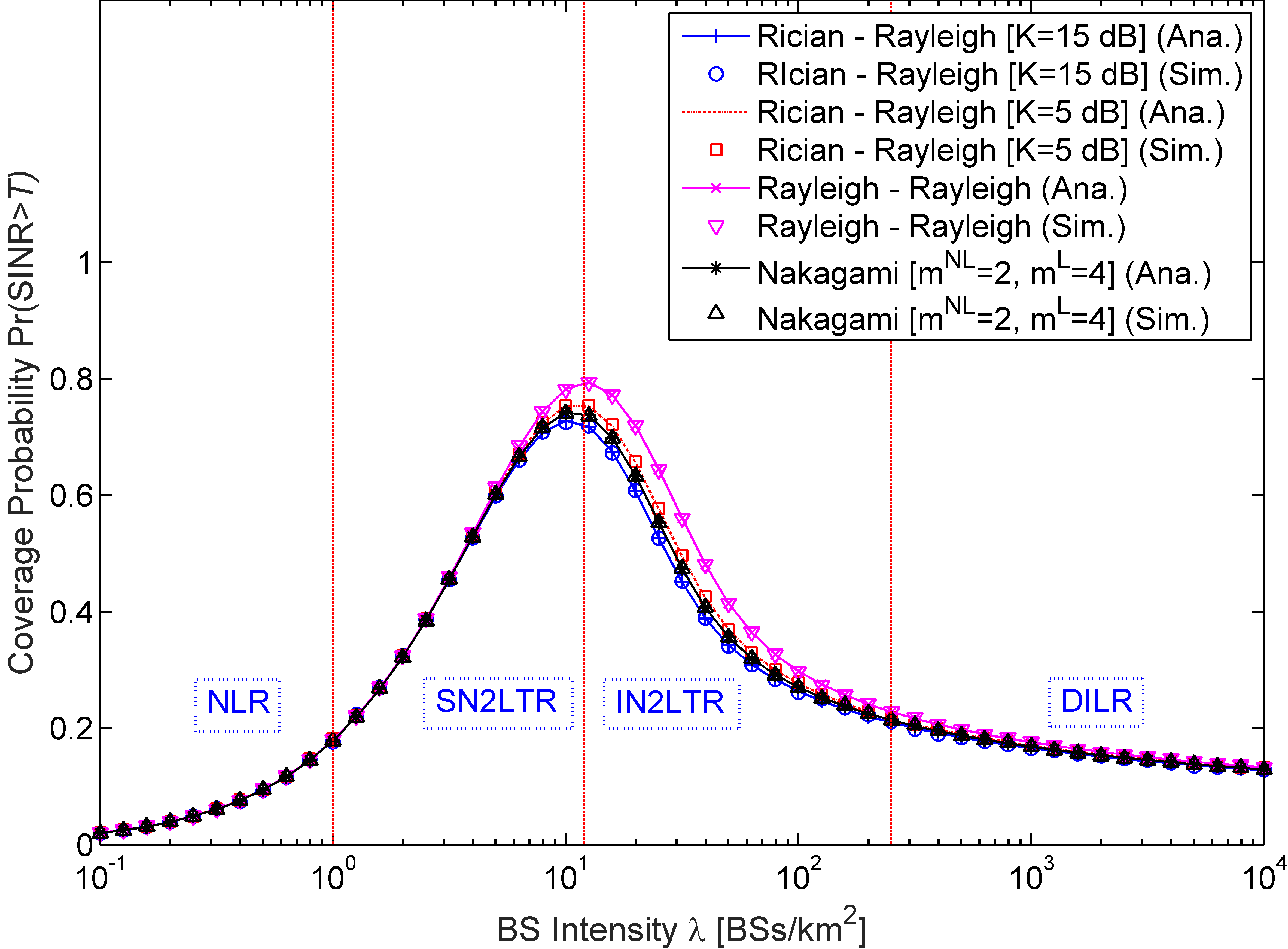
Figure 1: Coverage probability vs. BS intensity $\lambda$, $\eta=-95\textrm{ dBm}$, $T=0\textrm{ dB}.$

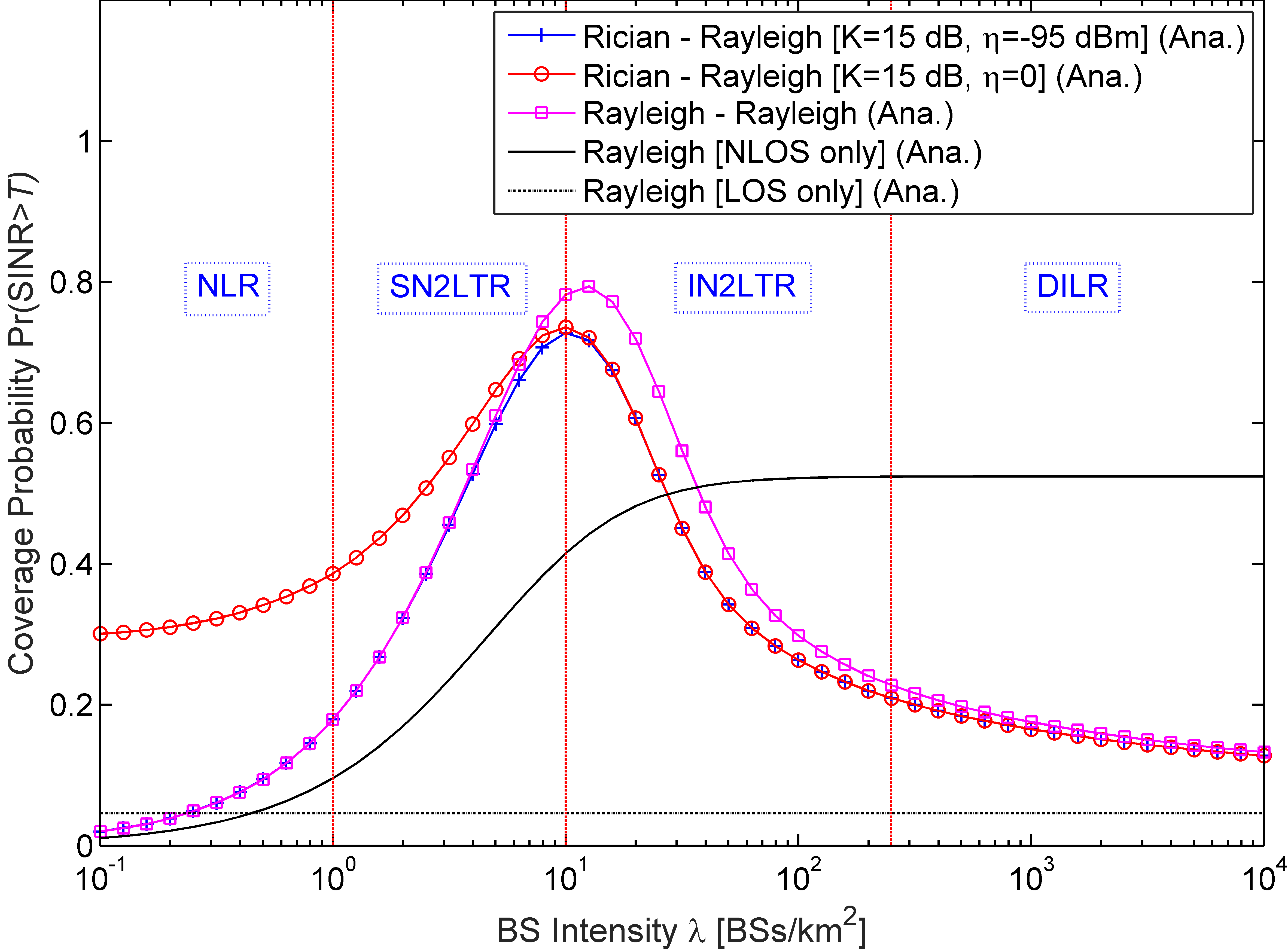
Figure 2: Coverage probability vs. BS intensity $\lambda$, $T=0\textrm{ dB}.$

The results of $p_{c}\left(\lambda,T\right)$ configured with $T=0\textrm{ dB}$ are plotted in Fig. 1 and Fig. 2. As can be observed from Fig. 1, the analytical results match the simulation results well, which validate the accuracy of our theoretical analysis. Note that in the case where both NLOS and LOS transmissions are concatenated with Rayleigh fading, the coverage probability is the highest among the interested cases. By contrast, in the case where NLOS transmission is concatenated with Rayleigh fading and LOS transmission is concatenated with Rician fading with $K=15\textrm{ dB}$, the coverage probability is the lowest. Meanwhile we should notice that the gap between the plotted curves is small, which suggests that multi-path fading has a minor impact on the coverage probability performance. In the following, we develop a more detailed analysis on the coverage probability according to $\lambda$, i.e.,

• Noise-Limited Regime (NLR): $\lambda\leqslant 1\textrm{ BSs/k$m^{2}$}$. In this regime, the typical MU is likely to have a NLOS path with the serving BS. The network in the NLR regime is very sparse and thus the interference can be ignored compared with the thermal noise if we use SINR as our performance metric. In this case, $\textrm{SINR}=\frac{S}{\eta}$ and the coverage probability will increase with the increase of $\lambda$ as the strongest received power ($S$) grows and noise power ($\eta$) remains the same. On the other hand, if we use SIR as our performance metric, the SIR coverage probability shows a flat trail in this regime as $\lambda$ increases (see Fig. 2). This is because the increase in the received signal power is almost counterbalanced by the increase in the aggregate interference power. Besides, as the aggregate interference power is smaller than noise power, the SIR coverage probability is larger than the SINR coverage probability.

• Signal NLOS-to-LOS-Transition Regime (SN2LTR): $\lambda\in(1,12]\textrm{ BSs/k$m^{2}$}$. In this regime, when $\lambda$ is small, the typical MU has a higher probability to connect to a NLOS BS; while when $\lambda$ becomes larger, the typical MU has an increasingly higher probability to connect to a LOS BS. That is to say, with the increase of $\lambda$, the typical MU is more likely to be associated with a LOS BS, i.e., the received signal transforms from a NLOS path to a LOS one. Even though the associated BS is LOS, the majority of interfering BSs are still NLOS in this regime and thus the SINR (or SIR) coverage probability continues growing. Besides, from this regime on, noise power has a negligible impact on coverage performance, i.e., the SCN becomes interference-limited.

• Interference NLOS-to-LOS-Transition Regime (IN2LTR): $\lambda\in(12,250]\textrm{ BSs/k$m^{2}$}$. In this regime, the typical MU is connected to a LOS BS with a high probability. However, different from the situation in the SN2LTR, the majority of interfering BSs experience transitions from NLOS to LOS path, which causes much more severe interference to the typical MU compared with interfering BSs with NLOS paths. As a result, the SINR (or SIR) coverage probability decreases with the increase of $\lambda$ because the transition of interference from NLOS path to LOS path causes a larger increase in interference compared with that in signal. Note that in this regime the coverage probability performance in our model exhibits a huge difference from that of the analysis in [15], which are indicated as “NLOS only” and “LOS only” in Fig. 2.

• Dense Interference-Limited Regime (DILR): $\lambda>250\textrm{ BSs/k$m^{2}$}$. In this regime, the network is extremely dense and LOS BSs dominate the SCNs. The SINR (or SIR) coverage probability becomes stable with the increase of BS intensity as any increase in the received LOS BS signal power is counterbalanced by the increase in the aggregate LOS BS interference power.

Remark 3.

Note that the boundaries between two adjacent regimes are quite qualitative which are worth further investigation.

Remark 4.

Note that the qualitative analysis of the coverage probability performance is in line with the findings in [4] (see the curve with square markers in Fig. 2).

IV-B Discussion on the Analytical Results of $\textrm{ASE}\left(\lambda\right)$

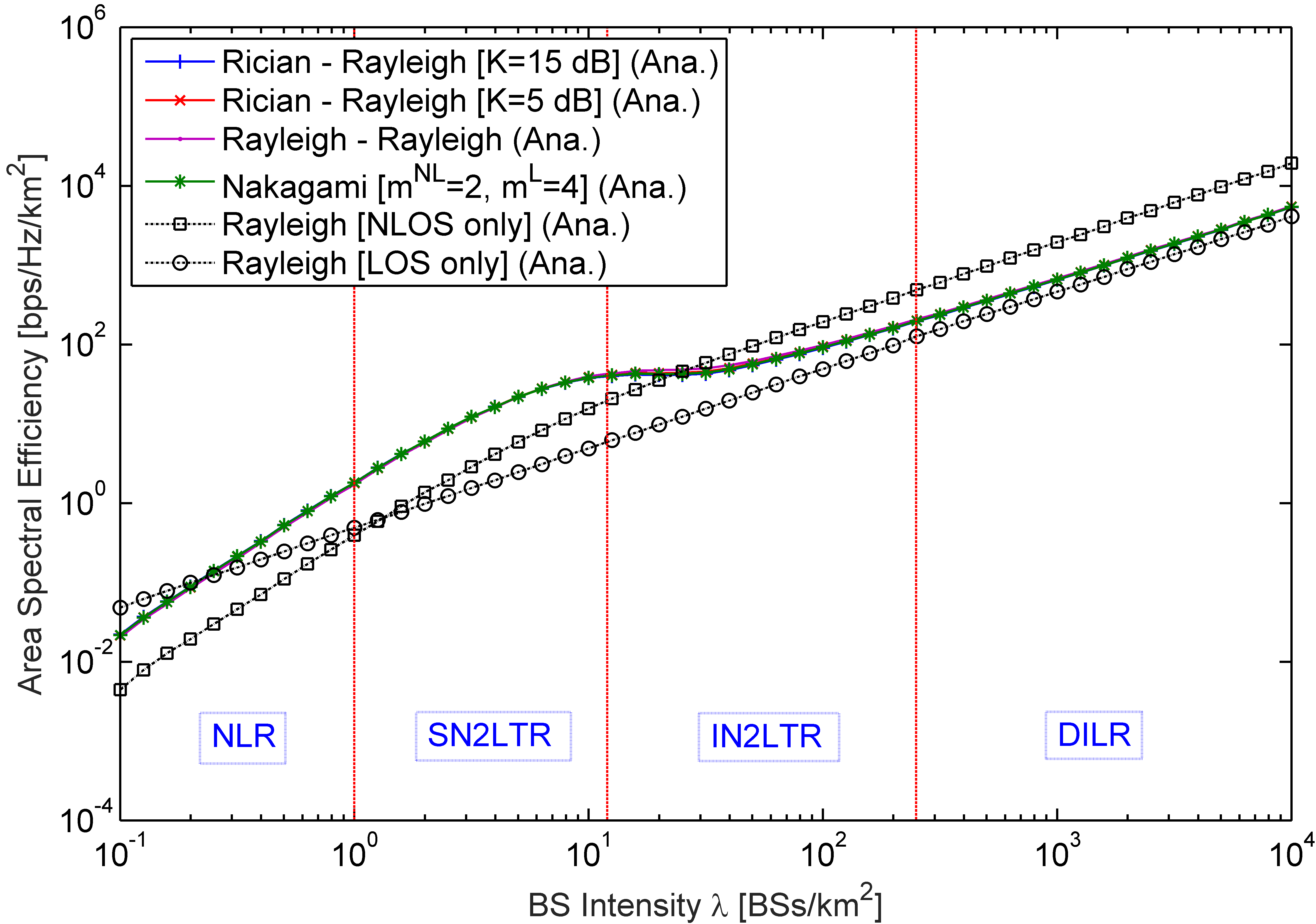
Figure 3: ASE vs. BS intensity $\lambda$, $\eta=-95\textrm{ dBm}$, $T=0\textrm{ dB}.$

In this subsection, the ASE with $T=0\textrm{ dB}$ is evaluated analytically, as $\textrm{ASE}\left(\lambda\right)$ is a function of $p_{c}\left(\lambda,T\right)$ which is analytically investigated in Eq. (25).

Fig. 3 illustrates the ASE with different fading models vs. $\lambda$. It is found that the ASE of the SCN incorporating both NLOS and LOS transmissions reveal a deviation from that of the analysis considering NLOS (or LOS) transmissions only [15]. Specifically, when the SCN is sparse and thus in the NLR or the SN2LTR, the ASE quickly increases with $\lambda$ because the network is generally noise-limited, and thus adding more small cells immensely benefits the ASE. When the network becomes dense, i.e., $\lambda$ enters the IN2LTR, which is the practical range of $\lambda$ for the existing 4G networks and the future 5G networks, the trend of the ASE performance is very interesting. First, when $\lambda\in(12,50]\textrm{ BSs/k$m^{2}$}$, the ASE exhibits a slowing-down in the rate of growth due to the fast decrease of the coverage probability at $\lambda\in(12,50]\textrm{ BSs/k$m^{2}$}$, as shown in Figs. 1 and 2. Second, when $\lambda>50\textrm{ BSs/k$m^{2}$}$, the ASE will pick up the growth rate since the decrease of the coverage probability becomes a minor factor compared with the increase of $\lambda$. When the SCN is extremely dense, e.g., $\lambda$ is in the DILR, the ASE exhibits a nearly linear trajectory with regard to $\lambda$ because both the signal power and the interference power are now LOS dominated, and thus statistically stable as explained before. Moreover, it can be observed that the change of the multi-path fading model has a minor impact on the ASE performance compared with the change of the path loss model.

V Conclusions and Future Work

In this paper, we proposed a unified framework to analyze the performance of the SCNs. In our analysis, we considered a practical path loss model that accounts for both NLOS and LOS transmissions. Furthermore, we adopted a generalized fading model, in which Rayleigh fading, Rician fading and Nakagami-$m$ fading can be treated in a unified framework. Different from existing work that does not differentiate NLOS and LOS transmissions, our results show that the co-existence of NLOS and LOS transmissions have a significant impact on the coverage probability and the ASE performance. Furthermore, our results establish for the first time that the performance of the SCNs can be divided into four regimes, according to the intensity of BSs, where in each regime the performance is dominated by different factors.

In our future work, both shadow fading and multi-path fading will be considered in our analysis which is more practical for the real network. Furthermore, heterogeneous networks (HetNets) incorporating both NLOS and LOS transmissions will also be investigated.

Appendix: Proof of Theorem 2

If we denote $\overline{R_{i}^{\textrm{NL}}}=R_{i}\cdot\left(B^{\textrm{NL}}h^{\textrm{NL}}\right)^{-1/\alpha^{\textrm{NL}}}$ and $\overline{R_{i}^{\textrm{L}}}=R_{i}\cdot\left(B^{\textrm{L}}h^{\textrm{L}}\right)^{-1/\alpha^{\textrm{L}}}$, $\left\{\overline{R_{i}^{\textrm{NL}}}\right\}_{i\in\mathbb{N}}$ (or $\left\{\overline{R_{i}^{\textrm{L}}}\right\}_{i\in\mathbb{N}}$) remains a PPP denoted by $\overline{\Phi^{\textrm{NL}}}$ (or $\overline{\Phi^{\textrm{L}}}$ ) according to the displacement theorem [9]. The intensity measure and intensities of $\overline{\Phi^{\textrm{NL}}}$ and $\overline{\Phi^{\textrm{L}}}$ are given by Eq. (13) - Eq. (16). The proof can be referred to [16, 17], which is omitted here. Next, we give the main proof of Theorem 2.

By invoking the law of total probability, the coverage probability can be divided into two parts, i.e., $p_{c}^{\textrm{NL}}\left(\lambda,T\right)$ and $p_{c}^{\textrm{L}}\left(\lambda,T\right)$, which denotes the conditional coverage probability given that the typical MU is associated with a BS in $\Phi^{\textrm{NL}}$ and $\Phi^{\textrm{L}}$, respectively. Moreover, denote by $\mathcal{P}^{\textrm{NL}}$ and $\mathcal{P}^{\textrm{L}}$ the strongest received signal power from BS in $\Phi^{\textrm{NL}}$ and $\Phi^{\textrm{L}}$, i.e., $\mathcal{P}^{\textrm{NL}}=\max\left(P_{i}^{\textrm{NL}}\right)$ and $\mathcal{P}^{\textrm{L}}=\max\left(P_{i}^{\textrm{L}}\right)$, respectively. Then by using the law of total probability, $p_{c}^{\textrm{L}}\left(\lambda,T\right)$ can be computed by

$$p_{c}^{\textrm{L}}\left(\lambda,T\right) =\Pr\left[\left(\textrm{SINR}^{\textrm{L}}>T\right)\cap\left(\mathcal{P}^{\textrm{L}}>\mathcal{P}^{\textrm{NL}}\right)\cap\mathcal{Y}^{\textrm{L}}\right]$$

$$=\mathbb{E}_{\mathcal{Y}^{\textrm{L}}}\biggl{\{}\underset{\textrm{II}}{\underbrace{\Pr\left[\left.\textrm{SINR}^{\textrm{L}}>T\right|\left(\mathcal{P}^{\textrm{L}}>\mathcal{P}^{\textrm{NL}}\right)\cap\mathcal{Y}^{\textrm{L}}\right]}}$$

$$\quad\,\times\underset{\textrm{I}}{\underbrace{\Pr\left[\left.\mathcal{P}^{\textrm{L}}>\mathcal{P}^{\textrm{NL}}\right|\mathcal{Y}^{\textrm{L}}\right]}}\biggr{\}},$$ (28)

where $\mathcal{Y}^{\textrm{L}}$ is the equivalent distance between the typical MU and the BS providing the strongest received signal power to the typical MU in $\Phi^{\textrm{L}}$, i.e., $\mathcal{Y}^{\textrm{L}}=\underset{\overline{R_{i}^{\textrm{L}}}\in\overline{\Phi^{\textrm{L}}}}{\arg\max}\left(\overline{R_{i}^{\textrm{L}}}\right)^{-\alpha^{\textrm{L}}}$, and also note that $\mathcal{P}^{\textrm{L}}=\left(\mathcal{Y}^{\textrm{L}}\right)^{-\alpha^{\textrm{L}}}$. Besides, Part I guarantees that the typical MU is connected to a LOS BS and Part II denotes the coverage probability conditioned on the proposed cell association scheme in Eq. (8). Next, Part I and Part II will be respectively derived separately. For Part I,

$$\quad\,\Pr\left[\left.\mathcal{P}^{\textrm{L}}>\mathcal{P}^{\textrm{NL}}\right|\mathcal{Y}^{\textrm{L}}\right]$$

$$=\Pr\left[\left.\left(\mathcal{Y}^{\textrm{L}}\right)^{-\alpha^{\textrm{L}}}>\left(\mathcal{Y}^{\textrm{NL}}\right)^{-\alpha^{\textrm{NL}}}\right|\mathcal{Y}^{\textrm{L}}\right]$$

$$=\Pr\left[\left.\mathcal{Y}^{\textrm{NL}}>\left(\mathcal{Y}^{\textrm{L}}\right)^{\alpha^{\textrm{L}}/\alpha^{\textrm{NL}}}\right|\mathcal{Y}^{\textrm{L}}\right]$$

$$\overset{\left(a\right)}{=}\exp\left[-\Lambda^{\textrm{NL}}\left(\left[0,\left(\mathcal{Y}^{\textrm{L}}\right)^{\alpha^{\textrm{L}}/\alpha^{\textrm{NL}}}\right]\right)\right],$$ (29)

where $\mathcal{Y}^{\textrm{NL}}$, similar to the definition of $\mathcal{Y}^{\textrm{L}}$, is the equivalent distance between the typical MU and the BS providing the strongest received signal power to the typical MU in $\Phi^{\textrm{NL}}$, i.e., $\mathcal{Y}^{\textrm{NL}}=\underset{\overline{R_{i}^{\textrm{NL}}}\in\overline{\Phi^{\textrm{NL}}}}{\arg\max}\left(\overline{R_{i}^{\textrm{NL}}}\right)^{-\alpha^{\textrm{NL}}}$, and also note that $\mathcal{P}^{\textrm{NL}}=\left(\mathcal{Y}^{\textrm{NL}}\right)^{-\alpha^{\textrm{NL}}}$, and $\left(a\right)$ follows from the void probability of a PPP.

For Part II, we know that $\textrm{SINR}=\frac{\mathcal{P}}{I+\eta}=\frac{\mathcal{P}}{I^{\textrm{NL}}+I^{\textrm{L}}+\eta},$ where $I^{\textrm{NL}}$ and $I^{\textrm{L}}$ denote the aggregate interference from NLOS BSs and LOS BSs, respectively. The conditional coverage probability is derived as follows

$$\quad\,\Pr\left[\left.\textrm{SINR}^{\textrm{L}}>T\right|\left(\mathcal{P}^{\textrm{L}}>\mathcal{P}^{\textrm{NL}}\right)\cap\mathcal{Y}^{\textrm{L}}\right]$$

$$=\Pr\left[\left.\frac{1}{\textrm{SINR}^{\textrm{L}}}<\frac{1}{T}\right|\left(\mathcal{P}^{\textrm{L}}>\mathcal{P}^{\textrm{NL}}\right)\cap\mathcal{Y}^{\textrm{L}}\right]$$

$$\overset{\left(a\right)}{=}\int_{x=0}^{1/T}\int_{\omega=-\infty}^{\infty}\frac{e^{-j\omega x}}{2\pi}\mathcal{F}_{\frac{1}{\textrm{SINR}^{\textrm{L}}}}\left(\omega\right)\textrm{d}\omega\textrm{d}x$$

$$=\int_{\omega=-\infty}^{\infty}\left[\frac{1-e^{-j\omega/T}}{2\pi j\omega}\right]\mathcal{F}_{\frac{1}{\textrm{SINR}^{\textrm{L}}}}\left(\omega\right)\textrm{d}\omega,$$ (30)

where $\textrm{SINR}^{\textrm{L}}$ denotes the SINR when the typical MU is associated with a LOS BS, the inner integral in $\left(a\right)$ is the conditional PDF of $\frac{1}{\textrm{SINR}^{\textrm{L}}}$, and $\mathcal{F}_{\frac{1}{\textrm{SINR}^{\textrm{L}}}}\left(\omega\right)$ denotes the conditional characteristic function of $\frac{1}{\textrm{SINR}^{\textrm{L}}}$ which is given by

$$\mathcal{F}_{\frac{1}{\textrm{SINR}^{\textrm{L}}}}\left(\omega\right)=\mathbb{E}_{\Phi}\left[\left.\exp\left(j\omega\frac{1}{\textrm{SINR}^{\textrm{L}}}\right)\right|\left(\mathcal{P}^{\textrm{L}}>\mathcal{P}^{\textrm{NL}}\right)\cap\mathcal{Y}^{\textrm{L}}\right]$$

$$=\mathbb{E}_{\Phi}\left[\left.e^{j\omega\left(I^{\textrm{NL}}+I^{\textrm{L}}+\eta\right)\left(\mathcal{Y}^{\textrm{L}}\right)^{\alpha^{\textrm{L}}}}\right|\left(\mathcal{P}^{\textrm{L}}>\mathcal{P}^{\textrm{NL}}\right)\cap\mathcal{Y}^{\textrm{L}}\right]$$

$$\overset{\left(a\right)}{=}\mathbb{E}_{\Phi^{\textrm{NL}}}\left\{\left.\exp\left[j\omega I^{\textrm{NL}}\cdot\left(\mathcal{Y}^{\textrm{L}}\right)^{\alpha^{\textrm{L}}}\right]\right|\left(\mathcal{P}^{\textrm{L}}>\mathcal{P}^{\textrm{NL}}\right)\cap\mathcal{Y}^{\textrm{L}}\right\}$$

$$\quad\,\times\mathbb{E}_{\Phi^{\textrm{L}}}\left\{\left.\exp\left[j\omega I^{\textrm{L}}\cdot\left(\mathcal{Y}^{\textrm{L}}\right)^{\alpha^{\textrm{L}}}\right]\right|\left(\mathcal{P}^{\textrm{L}}>\mathcal{P}^{\textrm{NL}}\right)\cap\mathcal{Y}^{\textrm{L}}\right\}$$

$$\quad\,\times e^{j\omega\eta\left(\mathcal{Y}^{\textrm{L}}\right)^{\alpha^{\textrm{L}}}},$$ (31)

where $\left(a\right)$ comes from the facts that $\Phi=\Phi^{\textrm{NL}}\cup\Phi^{\textrm{L}}$ and the mutual independence of $\Phi^{\textrm{NL}}$ and $\Phi^{\textrm{L}}$. Now by applying concepts from stochastic geometry, we will derive the term $\mathbb{E}_{\Phi^{\textrm{NL}}}\left\{\left.\exp\left[j\omega I^{\textrm{NL}}\left(\mathcal{Y}^{\textrm{L}}\right)^{\alpha^{\textrm{L}}}\right]\right|\left(\mathcal{P}^{\textrm{L}}>\mathcal{P}^{\textrm{NL}}\right)\cap\mathcal{Y}^{\textrm{L}}\right\}$ in Eq. (31) as follows

$$\quad\,\mathbb{E}_{\Phi^{\textrm{NL}}}\left\{\left.\exp\left[j\omega I^{\textrm{NL}}\cdot\left(\mathcal{Y}^{\textrm{L}}\right)^{\alpha^{\textrm{L}}}\right]\right|\left(\mathcal{P}^{\textrm{L}}>\mathcal{P}^{\textrm{NL}}\right)\cap\mathcal{Y}^{\textrm{L}}\right\}$$

$$\overset{\left(a\right)}{=}\mathbb{E}_{\overline{\Phi^{\textrm{NL}}}}\Biggl{\{}\left.\underset{i:\overline{R_{i}^{\textrm{NL}}}\in\overline{\Phi^{\textrm{NL}}}^{\prime}}{\prod}\exp\left[j\omega\cdot\left(\mathcal{Y}^{\textrm{L}}\right)^{\alpha^{\textrm{L}}}\left(\overline{R_{i}^{\textrm{NL}}}\right)^{-\alpha^{\textrm{NL}}}\right]\right|\bigl{(}\mathcal{P}^{\textrm{L}}$$

$$\quad\,>\mathcal{P}^{\textrm{NL}}\bigr{)}\cap\mathcal{Y}^{\textrm{L}}\Biggr{\}}$$

$$\overset{\left(b\right)}{=}\exp\left\{\int_{t=\left(\mathcal{Y}^{\textrm{L}}\right)^{\alpha^{\textrm{L}}/\alpha^{\textrm{NL}}}}^{\infty}\left[e^{j\omega\left(\mathcal{Y}^{\textrm{L}}\right)^{\alpha^{\textrm{L}}}t^{-\alpha^{\textrm{NL}}}}-1\right]\lambda^{\textrm{NL}}\left(t\right)\textrm{d}t\right\},$$ (32)

where in $\left(a\right)$, $\overline{\Phi^{\textrm{NL}}}^{\prime}=\overline{\Phi^{\textrm{NL}}}\setminus b\left(0,\left(\mathcal{Y}^{\textrm{L}}\right)^{\alpha^{\textrm{L}}/\alpha^{\textrm{NL}}}\right)$ and $\overline{R_{i}^{\textrm{NL}}}\in\overline{\Phi^{\textrm{NL}}}^{\prime}$ can guarantee the condition that $\mathcal{P}^{\textrm{L}}>\mathcal{P}^{\textrm{NL}}$, and $\left(b\right)$ is obtained by applying the probability generating functional (PGFL) [15, Eq. (3)] of the PPP. Similarly, the term $\mathbb{E}_{\Phi^{\textrm{L}}}\left\{\left.\exp\left[j\omega I^{\textrm{L}}\cdot\left(\mathcal{Y}^{\textrm{L}}\right)^{\alpha^{\textrm{L}}}\right]\right|\left(\mathcal{P}^{\textrm{L}}>\mathcal{P}^{\textrm{NL}}\right)\cap\mathcal{Y}^{\textrm{L}}\right\}$ in Eq. (31) is given by

$$\quad\,\mathbb{E}_{\Phi^{\textrm{L}}}\left\{\left.\exp\left[j\omega I^{\textrm{L}}\cdot\left(\mathcal{Y}^{\textrm{L}}\right)^{\alpha^{\textrm{L}}}\right]\right|\left(\mathcal{P}^{\textrm{L}}>\mathcal{P}^{\textrm{NL}}\right)\cap\mathcal{Y}^{\textrm{L}}\right\}$$

$$=\exp\left\{\int_{t=\mathcal{Y}^{\textrm{L}}}^{\infty}\left[e^{j\omega\left(\mathcal{Y}^{\textrm{L}}/t\right)^{\alpha^{\textrm{L}}}}-1\right]\lambda^{\textrm{L}}\left(t\right)\textrm{d}t\right\}\text{.}$$ (33)

Then the product of Part I and Part II in Eq. (28) can be obtained by substituting them with Eq. (29) – Eq. (33).

Finally, note that the value of $p_{c}^{\textrm{L}}\left(\lambda,T\right)$ in Eq. (28) should be calculated by taking the expectation with respect to $\mathcal{Y}^{\textrm{L}}$ in terms of its PDF, which is given as follows

$$f_{\mathcal{Y}^{\textrm{L}}}\left(y\right)=\frac{\textrm{d}}{\textrm{d}y}\left[1-\Pr\left(\mathcal{Y}^{\textrm{L}}>y\right)\right]=\lambda^{\textrm{L}}\left(y\right)\exp\left[-\Lambda^{\textrm{L}}\left(\left[0,y\right]\right)\right].$$ (34)

Given that the typical MU is connected to a NLOS BS, the conditional coverage probability $p_{c}^{\textrm{NL}}\left(\lambda,T\right)$ can be derived using the similar way as the above. In this way, the coverage probability is obtained by $p_{c}\left(\lambda,T\right)=p_{c}^{\textrm{L}}\left(\lambda,T\right)+p_{c}^{\textrm{NL}}\left(\lambda,T\right)$. Thus the proof is completed.

References

- [1] D. Lopez-Perez, M. Ding, H. Claussen, and A. H. Jafari, “Towards 1 gbps/ue in cellular systems: Understanding ultra-dense small cell deployments,” IEEE Commun. Surv. Tut., vol. 17, no. 4, pp. 2078–2101, Nov. 2015.
- [2] X. Ge, S. Tu, G. Mao, C. X. Wang, and T. Han, “5g ultra-dense cellular networks,” IEEE Wireless Commun., vol. 23, no. 1, pp. 72–79, Feb. 2016.
- [3] X. Ge, S. Tu, T. Han, Q. Li, and G. Mao, “Energy efficiency of small cell backhaul networks based on gauss-markov mobile models,” IET Networks, vol. 4, no. 2, pp. 158–167, Mar. 2015.
- [4] M. Ding, P. Wang, D. Lopez-Perez, G. Mao, and Z. Lin, “Performance impact of los and nlos transmissions in dense cellular networks,” IEEE Trans. Wireless Commun., vol. 15, no. 3, pp. 2365–2380, Mar. 2016.
- [5] M. D. Renzo, “Stochastic geometry modeling and analysis of multi-tier millimeter wave cellular networks,” IEEE Trans. Wireless Commun., vol. 14, no. 9, pp. 5038–5057, Sep. 2015.
- [6] S. Singh, M. N. Kulkarni, A. Ghosh, and J. G. Andrews, “Tractable model for rate in self-backhauled millimeter wave cellular networks,” IEEE J. Sel. Areas Commun., vol. 33, no. 10, pp. 2196–2211, Oct. 2015.
- [7] N. Blaunstein and M. Levin, “Parametric model of uhf/l-wave propagation in city with randomly distributed buildings,” in Proc. IEEE Antennas and Propagation Society International Symposium, vol. 3, Jun. 1998, pp. 1684–1687.
- [8] T. Bai, R. Vaze, and R. W. Heath, “Analysis of blockage effects on urban cellular networks,” IEEE Trans. Wireless Commun., vol. 13, no. 9, pp. 5070–5083, Sep. 2014.
- [9] F. Baccelli and B. Blaszczyszyn, Stochastic geometry and wireless networks. Now Publishers Inc, 2009.
- [10] T. Bai and R. W. Heath, “Coverage and rate analysis for millimeter-wave cellular networks,” IEEE Trans. Wireless Commun., vol. 14, no. 2, pp. 1100–1114, Feb. 2015.
- [11] F. Yilmaz and M. S. Alouini, “A unified mgf-based capacity analysis of diversity combiners over generalized fading channels,” IEEE Trans. Commun., vol. 60, no. 3, pp. 862–875, Mar. 2012.
- [12] 3GPP, “Tr 36.828 (v11.0.0): Further enhancements to lte time division duplex (tdd) for downlink-uplink (dl-ul) interference management and traffic adaptation,” Jun. 2012.
- [13] A. A. Kannan, B. Fidan, and G. Mao, “Robust distributed sensor network localization based on analysis of flip ambiguities,” in Proc. IEEE Globecom 2008, pp. 1–6.
- [14] B. Yang, G. Mao, X. Ge, H. H. Chen, T. Han, and X. Zhang, “Coverage analysis of heterogeneous cellular networks in urban areas,” in Proc. IEEE ICC, May 2016, pp. 1–6.
- [15] J. G. Andrews, F. Baccelli, and R. K. Ganti, “A tractable approach to coverage and rate in cellular networks,” IEEE Trans. Commun., vol. 59, no. 11, pp. 3122–3134, Nov. 2011.
- [16] B. Blaszczyszyn, M. K. Karray, and H. P. Keeler, “Using poisson processes to model lattice cellular networks,” in Proc. IEEE INFOCOM, Apr. 2013, pp. 773–781.
- [17] B. Yang, G. Mao, M. Ding, and X. Ge, “Performance analysis of dense scns with generalized shadowing/fading and nlos/los transmissions,” Jan. 2017. Available at: http://arxiv.org/abs/1701.01544.