Enstrophy Cascade in Decaying Two-Dimensional Quantum Turbulence

Abstract

We report evidence for an enstrophy cascade in large-scale point-vortex simulations of decaying two-dimensional quantum turbulence. Devising a method to generate quantum vortex configurations with kinetic energy narrowly localized near a single length scale, the dynamics are found to be well-characterised by a superfluid Reynolds number, $\operatorname{\mathrm{R\kern-0.44998pte}}_{\mathrm{s}}$, that depends only on the number of vortices and the initial kinetic energy scale. Under free evolution the vortices exhibit features of a classical enstrophy cascade, including a $k^{-3}$ power-law kinetic energy spectrum, and steady enstrophy flux associated with inertial transport to small scales. Clear signatures of the cascade emerge for $N\gtrsim 500$ vortices. Simulating up to very large Reynolds numbers ($N=32,768$ vortices), additional features of the classical theory are observed: the Kraichnan-Batchelor constant is found to converge to $C^{\prime}\approx 1.6$, and the width of the $k^{-3}$ range scales as $\operatorname{\mathrm{R\kern-0.44998pte}}_{\mathrm{s}}^{1/2}$. The results support a universal phenomenology underpinning classical and quantum fluid turbulence.

Quantum vortices in atomic Bose-Einstein condensates (BECs) offer the possibility not only to physically realize the point-vortex model envisaged by Onsager Onsager (1949), but also to observe and manipulate it at the level of individual quanta. Experimental techniques to controllably generate quantum vortices Kwon et al. (2014); Neely et al. (2010); Wilson et al. (2013); Samson et al. (2016), produce hard-wall trapping potentials containing large, uniform density condensates Henderson et al. (2009); Gauthier et al. (2016), and determine vortex circulation Seo et al. (2016) have all been recently demonstrated, and measurements of thermal friction coefficients Moon et al. (2015) and vortex annihilation and number decay Kwon et al. (2014); Neely et al. (2013) have already been made. For well-separated vortices, the point-vortex regime of two-dimensional quantum turbulence (2DQT) can be considered as a ‘stripped-down’ model of hydrodynamic turbulence with a definite number of degrees of freedom Billam et al. (2015), and thus studying the analogies between 2QDT and 2D classical turbulence (2DCT) may expand our understanding of universal turbulent phenomena. The recent experimental observation of a von Kármán vortex street and the transition to turbulence in the wake of a stirring obstacle Kwon et al. (2016), for example, adds to evidence that the classical Reynolds number concept may be generalized to quantum turbulence in frictionless superfluid flows Frisch et al. (1992); Finne et al. (2003); Reeves et al. (2015).

The enstrophy cascade of decaying 2DCT predicted by Batchelor Batchelor (1969) is a key process of classical turbulence for which the quantum analogue has remained unexplored. While much theoretical attention has focused on the inverse energy cascade of forced turbulence Numasato and Tsubota (2009); Numasato et al. (2010); Reeves et al. (2013); Chesler et al. (2013); Kobyakov et al. (2014); Siggia and Aref (1981) and macroscopic vortex clustering in 2DQT Billam et al. (2014); Simula et al. (2014); Yu et al. (2016), a clear demonstration of an enstrophy cascade has yet to be presented. A challenge to overcome in order to numerically demonstrate such a cascade in 2DQT is that of obtaining sufficiently large vortex number, initial spectral energy concentration, and range of wave numbers $k$, to identify the steep associated energy spectrum, $E(k)\propto k^{-3}$, over a significant range of scale space. The $k^{-3}$ scaling must also occur at large enough scales to distinguish it from the identical, physically unrelated, power-law scaling in the kinetic energy spectrum at the vortex-core scale Bradley and Anderson (2012a).

In this Letter we directly simulate an $N$-point-vortex model of decaying 2D quantum turbulence at large $N$. We devise a method of constructing an initial condition with a large energy contained within a single wavenumber, allowing us to simulate the 2DQT analog of a scenario where the existence of an enstrophy cascade is well-established in 2DCT Fox and Davidson (2010); Lindborg and Vallgren (2010). The initial states are found to be well-characterised by a superfluid Reynolds number $\operatorname{\mathrm{R\kern-0.44998pte}}_{\mathrm{s}}$ that depends only on the number of vortices and the initial wavenumber $k_{i}$. We show that under free evolution the characteristic $k^{-3}$ spectrum of the enstrophy cascade emerges for $N\gtrsim 500$, and the associated enstrophy and energy fluxes are found to agree with the Batchelor theory. By increasing $N$ up to $32,768$, additional key features of the theory are verified: the Kraichnan–Batchelor constant is found to be $C^{\prime}\approx 1.6$, close to the accepted classical value, and the length of the inertial range scales as $\operatorname{\mathrm{R\kern-0.44998pte}}_{\mathrm{s}}^{1/2}$.

Background.— Turbulent flows at large Reynolds numbers ($\operatorname{\mathrm{R\kern-0.44998pte}}$) can spontaneously develop self-similar cascade solutions, in which quantities are conservatively transported across a subregion of scale space called the inertial range. Two-dimensional turbulence cannot support the usual Kolmogorov energy cascade of 3D turbulence, since the mean square vorticity, or enstrophy is unable to be amplified through vortex stretching. However, Batchelor Batchelor (1969) hypothesised that in 2D the enstrophy itself could therefore undergo a cascade, from small to large wavenumbers, via a filamentation of vorticity patches. The enstrophy cascade is signified by a kinetic energy spectrum $E(k)=C^{\prime}\eta^{2/3}k^{-3}$, where $\eta$ is the enstrophy dissipation rate (assumed equal to the enstrophy flux in the inertial range), and $C^{\prime}$ is the Kraichnan–Batchelor constant. The lossless cascade terminates at a dissipation wavenumber $k_{d}\sim k_{i}\operatorname{\mathrm{R\kern-0.44998pte}}^{1/2}$, at which viscous dissipation becomes important. The enstrophy casade must be accompanied by a drift of energy to small wavenumbers, in order to be simultaneously consistent with the conservation laws of energy and enstrophy.

Model.— We consider a quantum fluid, such as a BEC, characterized by healing length $\xi$ and speed of sound $c$, carrying quantized vortices of charge $\kappa_{i}=\pm 1$ and circulation $\Gamma_{i}=\kappa_{i}\Gamma$ . For a quasi-2D system, vortex bending is suppressed and the dynamics become effectively two-dimensional Rooney et al. (2011). In the low Mach number limit, where the average intervortex distance $\ell$ is much greater than the healing length $\xi$, interactions between vortices and density fluctuations can be ignored on scales $\gtrsim\xi$. In this limit a fully compressible (e.g., Gross-Pitaevskii Blakie et al. (2008)) description, that complicates interpretation of fluxes Billam et al. (2015), is not needed. Instead, the motion of the $i$th quantum vortex, located at $\mathbf{r}_{i}$, can be described by a dissipative point-vortex model Törnkvist and Schröder (1997) with compressible effects (at length scales $\lesssim\xi$) added phenomenologically Billam et al. (2015); Kim et al. (2016). The motion of the $i$th quantum vortex, located at $\mathbf{r}_{i}$, is given by

$$\frac{d\mathbf{r}_{i}}{dt} =\mathbf{v}_{i}+\mathbf{w}_{i};\;\;\mathbf{v}_{i}=\sum_{j=1,j\neq i}^{N}\mathbf{v}_{i}^{(j)};\;\;\mathbf{w}_{i}=-\gamma\kappa_{i}\hat{\mathbf{e}}_{3}\times\mathbf{v}_{i},$$ (1)

where $\gamma$ is the dissipation rate, $\mathbf{\hat{e}}_{3}$ is a unit vector perpendicular to the fluid plane, and $\mathbf{v}_{i}$ and $\mathbf{w}_{i}$ are the conservative and dissipative parts of the velocity respectively. The dissipation rate $\gamma$ arises from thermal friction due to the normal fluid component, here assumed to be stationary Moon et al. (2015). Phenomenologically, we remove opposite-sign vortex pairs separated by less than $\xi$ (modelling dipole annihilation), and smoothly increase the dissipation $\gamma$ for same-sign vortex pairs as their separation decreases to around $\xi$ (modelling sound radiation by accelerating vortices Pismen (1999)). Details can be found in the Supplemental Material Sup , or Ref. Billam et al. (2015).

The velocity of the $i$th vortex due to the $j$th, $\mathbf{v}_{i}^{(j)}$, is obtained from a Hamiltonian point-vortex model subject to appropriate boundary conditions. As usually considered classically Lilly (1969, 1971); Brachet et al. (1988); Vallgren and Lindborg (2011), we will consider a doubly-periodic square box with side length $L\gg\xi$, for which Weiss and McWilliams (1991)

$$\mathbf{v}_{i}^{(j)}=\frac{\pi c\kappa_{j}}{(L/\xi)}\sum_{m=-\infty}^{\infty}\left(\begin{array}[]{c}\frac{-\sin(y_{ij}^{\prime})}{\cosh(x_{ij}^{\prime}-2\pi m)-\cos(y_{ij}^{\prime})}\\ \frac{\sin(x_{ij}^{\prime})}{\cosh(y_{ij}^{\prime}-2\pi m)-\cos(x_{ij}^{\prime})}\end{array}\right),$$ (2)

where $(x_{ij}^{\prime},y_{ij}^{\prime})/(2\pi/L)\equiv\mathbf{r}_{ij}\equiv\mathbf{r}_{i}-\mathbf{r}_{j}$. The absence of a physical boundary offers the usual advantage: vortices cannot reach their own images, enforcing conservation of the (zero) net vorticity. This helps achieve statistical homogeneity and isotropy, as required for comparisons with Batchelor’s theory.

Spectrum.— The kinetic energy spectrum (per unit mass) in the periodic box is given by Billam et al. (2014)

$$E(\mathbf{k})={} E_{\rm self}(\mathbf{k})+E_{\rm int}(\mathbf{k})$$ (3)

$$={} \frac{\Gamma^{2}}{8(\pi kL)^{2}}\left[N+2\sum_{i=1}^{N}\sum_{j=i+1}^{N}\langle\kappa_{i}\kappa_{j}\cos(\mathbf{k}\cdot\mathbf{r}_{ij})\rangle\right],$$ (4)

where $\mathbf{k}=(n_{x}\Delta k,n_{y}\Delta k)$ for $n_{x},n_{y}\in\mathbb{Z}$, $\Delta k=2\pi/L$, and $\langle\,\cdot\,\rangle$ denotes ensemble averaging. The average kinetic energy is $\sum_{\mathbf{k}}\;E(\mathbf{k})(\Delta k)^{2}=E_{\rm self}+E_{\rm int}$. The self-energy term is, for fixed $N$, a cutoff-dependent constant, set by $L$ and the vortex core structure at wavenumbers $k\gtrsim\xi^{-1}$ Billam et al. (2014) (not considered here). The time evolution of $E(\mathbf{k})$ governs the spectral transport of kinetic energy:

$$\frac{dE(\mathbf{k})}{dt} =T(\mathbf{k})+D(\mathbf{k}),$$ (5)

where $T(\mathbf{k})$ is the transfer function, given by

$$T(\mathbf{k}) =-\frac{\Gamma^{2}}{4(\pi kL)^{2}}\sum_{i=1}^{N}\sum_{j=i+1}^{N}\langle\kappa_{i}\kappa_{j}\sin(\mathbf{k}\cdot\mathbf{r}_{ij})\mathbf{k}\cdot(\mathbf{v}_{i}-\mathbf{v}_{j})\rangle,$$ (6)

and $D(\mathbf{k})$ is the dissipation spectrum, obtained from Eq. (6) by setting $\mathbf{v}\rightarrow\mathbf{w}$. As usual, the enstrophy and energy spectra are related via $\Omega(\mathbf{k})=2k^{2}E(\mathbf{k})$. Like its classical counterpart, the superfluid transfer function $T(\mathbf{k})$ conservatively redistributes energy, with $\sum_{\mathbf{k}}T(\mathbf{k})(\Delta k)^{2}=0$. The dissipation spectrum $D(\mathbf{k})$ governs the rate of energy loss: $\sum_{\mathbf{k}}D(\mathbf{k})(\Delta k)^{2}=dE/dt<0$. The one-dimensional (angularly integrated) spectral measures $E(k)=\int d\phi_{k}kE(\mathbf{k})$ etc., are analysed by defining a discrete angular integral over a ring of wavenumbers: $\tilde{f}(n\Delta k)=\sum_{\mathbf{k}\in\mathcal{D}_{n}}f(\mathbf{k})\,\Delta k$, where $\mathcal{D}_{n}=\{\mathbf{k}\,|\,(n-1/2)\Delta k\leq|\mathbf{k}|\leq(n+1/2)\Delta k\}$, and $n=1,2,\ldots$. Hence we may define the discrete energy and enstrophy fluxes Kraichnan (1967); Kraichnan and Montgomery (1980)

$$\tilde{\Pi}_{\epsilon}\left(n\Delta k\right) =-\textstyle\sum_{m=1}^{n}\tilde{T}(m\Delta k)\,\Delta k,$$ (7)

$$\tilde{\Pi}_{\omega}\left(n\Delta k\right) =-2\textstyle\sum_{m=1}^{n}(m\Delta k)^{2}\tilde{T}(m\Delta k)\,\Delta k,$$ (8)

that represent the instantaneous energy and enstrophy fluxes through the $k$-space bin $|\mathbf{k}|=n\Delta k$ due to the conservative interactions. Turbulent cascades can be expected to develop when $\gamma\ll 1$ and $T(\mathbf{k})$ is large, allowing a lossless inertial range to be established over some range of $k$.

Initial condition.— Although at sufficiently large Reynolds number any initial state should tend towards the $k^{-3}$ similarity state, the simplest initial state has all the kinetic energy localized near an initial wavenumber, as is often considered classically Lilly (1971); Lindborg and Vallgren (2010). However, it is not immediately evident from Eq. (16) how such a state can be created with quantum vortices. Here we devise a simple method to create a superfluid analog of these states: We define a set of wavenumbers $\mathcal{D}_{i}$ that form a shell of width $w$ localised around a chosen initial wavenumber $k_{i}$: $\mathcal{D}_{i}=\{\mathbf{k}\,|\,k_{i}-w/2\leq|\mathbf{k}|\leq k_{i}+w/2\}$. Each mode in $\mathcal{D}_{i}$ is occupied with a random complex phase $\theta(\mathbf{k})$, uniformly sampled on $[0,2\pi]$ to define a (Hermitian) vorticity field $\hat{\omega}(\mathbf{k})=e^{i\theta(\mathbf{k})}$ if $\mathbf{k}\in\mathcal{D}_{i}$ and $\hat{\omega}(\mathbf{k})=0$ otherwise. The real-space vorticity field, $\omega(\mathbf{r})=\int d^{2}\mathbf{k}\;e^{i\mathbf{k}\cdot\mathbf{r}}\hat{\omega}(\mathbf{k})$, is then separated into positive and negative regions $\omega_{\pm}(\mathbf{r})$ as $\omega_{+}(\mathbf{r})=\omega(\mathbf{r})$ if $\omega(\mathbf{r})>0$ and $\omega_{+}(\mathbf{r})=0$ otherwise, and similarly for $\omega_{-}(\mathbf{r})$. The components are then normalised to unity [$\int d^{2}\mathbf{r}\omega_{\pm}(\mathbf{r})=1$], and used as probability distributions to create an $N$-point-vortex initial condition via rejection sampling. This procedure creates an initial condition with the vast majority of the interaction energy contained within one $k$-mode [Fig. 1(a), inset], even for small vortex numbers $N\sim 10^{2}$.

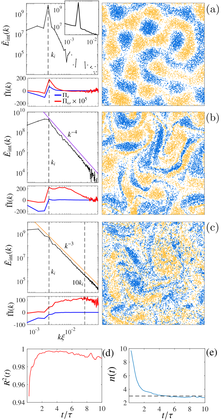
Figure 1: (color online). Vorticity distributions, kinetic energy spectra, and fluxes (in units of $\Gamma^{2}/4\pi L^{2}$) for $N=16,384$ at (a) $t\approx 0.25\tau$, (b) $t\approx 1.85\tau$, and (c) $t\approx 4\tau$. In the top panel, at high $k$, $E_{\rm int}(k)$ is comparatively small and oscillates about zero. The negative values cannot be shown on the log scale, causing the broken data line. Inset shows the full spectrum, $E_{\rm self}(k)+E_{\rm int}(k)$, at $t=0$. (d) and (e) show, respectively, the $R^{2}$ goodness of fit value and the best-fit slope $n$ [$E(k)\sim k^{-n}$] as functions of time, obtained from a linear fit to the log-log data over the decade of wavenumbers marked in (c). Values are averaged over $4$ runs and $9$ time samples with time-spacing $\delta t\approx\tau/20$. The dashed line in (e) shows $n=3$.

Dynamics.— Starting from the initial conditions described above, we simulate the dynamics of neutral point-vortex systems with fixed $L=10^{4}\xi$, fixed dissipation $\gamma=10^{-4}$ Bradley and Anderson (2012a); Stagg et al. (2015), and vortex numbers $N=2^{n},n=\{9,10,\dots,15\}$ . The system can be characterised by the superfluid Reynolds number $\mathrm{Re_{s}}$ Onsager (1953) and the eddy turnover time $\tau$

$$\operatorname{\mathrm{R\kern-0.44998pte}}_{\mathrm{s}} =\frac{E_{\rm int}^{1/2}L_{i}}{\Gamma},\quad\quad\tau=\frac{L_{i}}{\mathrm{v}_{\rm rms}},$$ (9)

where $L_{i}=2\pi/k_{i}$, and $\mathrm{v}_{\rm rms}$ is the root-mean-square vortex velocity. In the Supplemental Material Sup we show that for a wide range of the localised initial conditions, $E_{\rm int}$ is well-approximated by

$$E_{\rm int} =A\times\left(\frac{\Gamma^{2}}{4\pi L^{2}}\right)\left(\frac{N}{k_{i}}\right)^{2}(\Delta k)^{2},$$ (10)

where $A=\mathrm{const.}\approx 0.25$. Neglecting unimportant constant factors, this yields a remarkably simple formula for $\mathrm{Re_{s}}$ as the ratio of two dimensionless quantities,

$$\mathrm{Re_{s}} =N/n_{i}^{2},$$ (11)

where $n_{i}\equiv k_{i}/\Delta k$ is the dimensionless initial wavenumber. To maximise $\mathrm{Re_{s}}$ while still maintaining approximate isotropy, we thus set $L_{i}=L/4$. Since $\mathrm{Re_{s}}$ is independent of the value of $w$, we choose the narrowest window, $w=\Delta k$. We directly simulate the point-vortex model [Eqs. (12) and (2)] and compute time- and ensemble-averaged spectra and fluxes [Eqs. (16)–(8)], using GPU codes NVIDIA Corporation (2014) that allow us to evaluate the full $N$-body problem for very large $N$.

Fig. 1(a)-(c) shows the dynamics of the vortices, kinetic energy spectra, and fluxes for $N=16,384$. The qualitative behaviour is similar for all $N$ considered, but naturally large $N$ yields cleaner results. Movies for some cases are provided in the Supplemental Material Sup . Very early times [Fig. 1(a)] show the spectrum rapidly spreads from the initial state well-localised at $k_{i}=4(\Delta k)$ [Fig. 1(a), inset]. A linear fit to the log-log spectrum indicates that $t\approx 2\tau$, where the $R^{2}$ goodness of fit plateaus near unity [Fig  1(d)], marks the onset of power-law scaling. At the onset, the spectrum agrees quite well with the Saffman Saffman (1992) scaling $k^{-4}$, consistent with the formation of sharp, isolated vorticity-gradient filaments [Fig. 1, (b)]. These filaments are repeatedly stretched and packed, and the spectral slope gradually transitions, settling to the $k^{-3}$ scaling from $t\sim 4\tau$ onwards [Fig. 1, (c,e)], maintaining a high goodness of fit, $R^{2}>0.988$ [Fig 1(d)]. A transition from $k^{-4}$ to $k^{-3}$ scaling was also reported in pseudospectral Navier-Stokes simulations of decaying 2D turbulence Brachet et al. (1988). Note that in Fig. 1 only the interaction term $E_{\rm int}(k)$ is shown, as the self-energy term can only ever contribute a trivial $N/k$ scaling.

Inspection of the energy and enstrophy fluxes confirms the directions of spectral transport. The early developing stages of evolution [Fig. 1(b)] clearly demonstrate a development of a negative energy flux (indicating flow to low $k$) and positive enstrophy flux (indicating flow to high $k$) in the mutually exclusive wavenumber regions $k<k_{i}$ and $k>k_{i}$ respectively. The $k^{-3}$ spectrum [Fig. 1(c)] is corroborated by a nearly constant enstrophy flux over approximately one decade of wavenumbers, providing a means to estimate $\eta$ and determine the Kraichnan-Batchelor constant via the so-called compensated kinetic energy spectrum: $C^{\prime}=E(k)k^{3}/\eta^{2/3}$, where $\eta=\Pi_{\omega}$ averaged over $k$, time window, and ensemble.

Fig. 2 shows the compensated spectrum for different $N$ at $t\sim 4\tau$. The $k^{-3}$ scaling is observed to some degree for all $N$ considered, albeit over less than a decade for small $N$ ($\sim 0.7$ decades for $N=512$). However the quality and range of the scaling increases dramatically as $N$ is increased. For smaller $N$, $C^{\prime}$ is quite large ($C^{\prime}\approx 3.8$) , but as $N$ increases $C^{\prime}$ decreases and tends towards a constant value $C^{\prime}\approx 1.6$. A simulation with $N=16,384$ and $k_{f}=8(\Delta k)$ yielded $C^{\prime}\approx 2.0$, in good agreement with $N=4096$, $k_{f}=4(\Delta k)$, that has the same $\operatorname{\mathrm{R\kern-0.44998pte}}_{\mathrm{s}}$ and yielded $C^{\prime}\approx 1.9$. The scaling range is found to persist up to $k_{\ell}=2\pi/\ell$, the wavenumber associated with the average intervortex distance $\ell=L/N^{1/2}$. Notice that for $N\geq 16,384$ this means the compensated spectrum is constant over a significant range of roughly 1.5 decades above the initial wavenumber. Above $k_{\ell}$, the interaction spectrum quickly decreases, indicating a transition from many-vortex to single-vortex physics.

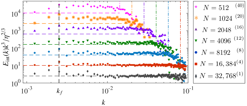
Figure 2: Compensated kinetic energy spectra for a range of $N$, averaged over ensemble and a time window $\sim 0.5\tau$. For clarity the spectra are vertically shifted by increasing powers of $4$. The horizontal dashed lines shows the value $C^{\prime}=1.6$ (also vertically shifted for comparison at different $N$). Dash-dot lines indicate the intervortex distance wavenumber $k_{\ell}$ at different $N$ (see text). In the legend the bracketed superscripts indicate the number of independent realisations used in the ensemble average.

Discussion.— It appears that the basic phenomenology of the decaying enstrophy cascade can indeed be seen in 2DQT. For large $\operatorname{\mathrm{R\kern-0.44998pte}}_{\mathrm{s}}$, we find a Kraichnan-Batchelor constant $C^{\prime}\approx 1.6$ close to the accepted value for a classical fluid, $C^{\prime}=1.4$ Paret et al. (1999); Lindborg and Vallgren (2010). Similarly, the Kolmogorov constant in 3D has been found to be the same above and below the $\lambda$-transition in superfluid He⁴ Barenghi et al. (2014). Our observation of greater values of $C^{\prime}$ at lower $\operatorname{\mathrm{R\kern-0.44998pte}}_{\mathrm{s}}$ (although with greater uncertainties) suggests that fewer available degrees of freedom result in less efficient spectral transport. Importantly, our results show that $\operatorname{\mathrm{R\kern-0.44998pte}}_{\mathrm{s}}$ as defined in Eq. (11) quantifies the degree of turbulence very well, and can be used to estimate the range of the enstrophy cascade. Since $\operatorname{\mathrm{R\kern-0.44998pte}}_{\mathrm{s}}=N(\Delta k/k_{i})^{2}$, our results exhibit the same power-law range scaling as a classical fluid: $k_{\ell}/k_{i}\sim\operatorname{\mathrm{R\kern-0.44998pte}}_{\mathrm{s}}^{1/2}$. Similarly, a recent experiment Babuin et al. (2014) found $\ell^{-1}\sim\operatorname{\mathrm{R\kern-0.44998pte}}_{\mathrm{s}}^{3/4}$ in 3DQT (for an appropriately defined $\operatorname{\mathrm{R\kern-0.44998pte}}_{\mathrm{s}}$), similar to the dissipation scale in the Kolmogorov energy casade. However, here the cascade terminates due to a crossover from many-vortex to single-vortex physics, rather than due to dissipative effects. The sudden drop in $E_{\rm int}(k)$ at $k_{\ell}$ suggests that the point-vortex system can effectively be truncated at wavenumbers $k\sim k_{\ell}$, as was qualitatively argued by Kraichnan Kraichnan (1975).

Further study of how dual inverse-energy and direct-enstrophy cascades Kraichnan (1967); Leith (1968) could manifest in forced 2DQT is certainly warranted. A study of the inverse energy cascade using a forced point-vortex model Siggia and Aref (1981) found the Kraichnan-Kolmogorov constant to be twice the accepted value. However in Ref. Siggia and Aref (1981) forcing was introduced by essentially reversing the sign of $\gamma$. Adapting our rejection-sampling method to dynamically introduce vorticity instead could provide a more physical model, roughly corresponding to turbulence generated by a stirring grid in a 2D quantum fluid Skaugen and Angheluta (2016); Sommeria (1986); Rutgers (1998). Studying the forced case would allow exploration of conditions under which both cascades coexist in the point-vortex system, and of intermittency effects Paret et al. (1999). It will also be interesting to explore the relation between the enstrophy cascade observed here and the anomalous scaling at non-thermal fixed points in compressible decaying 2DQT Karl and Gasenzer (2016); Schole et al. (2012).

Finally, let us discuss the prospect of observing the cascade in atomic condensates. The main challenge would be creating a system large enough relative to the healing length, $\xi$. Currently, experimental setups have produced pure, stable condensates of up to $N_{a}\sim 10^{8}$ atoms with atomic number densities $n_{0}\sim 10^{14}$ cm^-3, using ²³Na Streed et al. (2006). The $s$-wave scattering length $a_{s}\approx 2.8$nm Streed et al. (2006), gives $\xi=1/\sqrt{4\pi n_{0}a_{s}}\approx 0.53\mu\mathrm{m}$. Assuming such parameters in a uniform quasi-2D system of volume $L^{2}h$, with thickness $h\sim 6.6\xi$ Kwon et al. (2014), gives $L/\xi\approx 1000$. This would allow $N=512$, since here $\mathrm{v_{rms}}/c\approx 0.025$ and hence the system size could be reduced to $L/\xi\sim 850$ without invalidating the incompressibility assumption $\mathrm{v}_{\mathrm{rms}}/c\lesssim 0.3$ [in Eqs. (12) and (2) $\{\mathbf{x},L\}\rightarrow\lambda\{\mathbf{x},L\}$ gives $\mathbf{v}\rightarrow\lambda^{-1}\mathbf{v}$, $t\rightarrow\lambda^{2}t$]. However, a system with $L/\xi\sim 1000$ would correspond to a cloud $\sim$$500$ $\mu$m across, an order of magnitude larger than in current experiments. Recent experimental 2DQT studies have acheived $L\sim 500\xi$ and $N\sim 80$ vortices in harmonically confined systems Kwon et al. (2014); Moon et al. (2015); Kwon et al. (2015), and hard-wall traps Gaunt et al. (2013); Navon et al. (2016) with $L/\xi\gtrsim 200$ Gauthier et al. (2016). Ultracold Fermi gases, with a much shorter healing length, may also be a viable alternative Bulgac et al. (2016). Condensate lifetimes $T>60$ s are common Kwon et al. (2014), giving $T\approx 4.6\times 10^{5}$ $\xi/c$, or $T/\tau\approx 460$, greatly exceeding the requirements here. Some further additional freedom is possible by decreasing $\xi\propto a_{s}^{-1/2}$ through a Feshbach resonance Inouye et al. (1998); Chin et al. (2010), although this would eventually enhance three-body losses Stenger et al. (1999). Controlled stirring protocols show promise for efficient cluster injection Reeves et al. (2015); Stagg et al. (2015); Kwon et al. (2014). While challenging, the required experimental conditions are not inaccessible.

Conclusion.— We have numerically observed signatures of an enstrophy cascade in decaying 2DQT, including a $k^{-3}$ power-law spectrum, constant enstrophy flux over a wide inertial range, and a Kraichnan-Batchelor constant converging to $C^{\prime}\approx 1.6$ for large vortex number. We have shown that the extent of the inertial range scales as $\operatorname{\mathrm{R\kern-0.44998pte}}_{\mathrm{s}}^{1/2}$ for a suitably-defined superfluid Reynolds number, $\operatorname{\mathrm{R\kern-0.44998pte}}_{\mathrm{s}}$, that depends only on the number of vortices and the length scale where kinetic energy is initially concentrated. The relevance of the classical cascade theory for describing decaying 2DQT suggests an underlying universality of decaying turbulence phenomena. Signatures of the enstrophy cascade become observable for systems of a few hundred vortices, and may soon be within reach of cold-atom 2DQT experiments.

We thank B. P. Anderson for many stimulating discussions and A. J. Groszek for valuable comments. A.S.B was supported by a Rutherford Discovery Fellowship administered by the Royal Society of New Zealand.

Supplemental Material

I Point-vortex simulations

As described in the main text, we simulate a weakly-dissipative point-vortex model with added phenomenological treatment of the main effects arising from compressibility of a quantum fluid when vortices approach each other at healing-length scales. This model was described in Ref. Billam et al. (2015); we summarize it here for convenience.

We consider a dissipative point-vortex model in which the motion of the $i$th quantum vortex, located at $\mathbf{r}_{i}$, is given by

$$\frac{d\mathbf{r}_{i}}{dt} =\mathbf{v}_{i}+\mathbf{w}_{i};\;\;\mathbf{v}_{i}=\sum_{j=1,j\neq i}^{N}\mathbf{v}_{i}^{(j)};\;\;\mathbf{w}_{i}=-\gamma\kappa_{i}\hat{\mathbf{e}}_{3}\times\mathbf{v}_{i},$$ (12)

where $\gamma$ is the background dissipation rate, $\mathbf{\hat{e}}_{3}$ is a unit vector perpendicular to the fluid plane, and $\mathbf{v}_{i}$ and $\mathbf{w}_{i}$ are the conservative and dissipative parts of the velocity respectively [see Eq. (1) in the main text]. The added phenomenolgical treatment has two aspects:

(a) To model the annihilation of closely-spaced vortex – antivortex dipoles, at the end of every simulation timestep we remove any opposite-circulation vortex pairs that are separated by distances less than the healing length $\xi$.

(b) To model the effects of sound radiation by closely-spaced same-circulation vortex pairs, for a vortex $i$ with nearest same-circulation neighbour $s$ located a distance $r_{is}$ away we compute a local disspation rate

$$\gamma_{i}=\mathrm{max}\left(\exp\left[\ln(\gamma)\frac{r_{is}-r_{1}}{r_{2}-r_{1}}\right],\gamma\right)\,.$$ (13)

When computing the evolution of vortex $i$, we replace the background dissipation rate $\gamma$ with the local dissipation rate $\gamma_{i}$ in Eq. (12). We choose $r_{2}=\xi$ and $r_{1}=0.1\xi$, although the results are insensitive to the precise values of these parameters. Increasing $r_{2}$ and $r_{1}$ by an order of magnitude did not qualitatively alter the results presented Billam et al. (2015).

We emphasise that the inclusion of dissipation in our model is important to describe the dynamics of typical experimental quantum fluids. For example, in the case of BEC experiments Eq. (12) can be derived from the damped Gross-Pitaevskii equation Billam et al. (2015),

$$i\frac{\partial\psi}{\partial t}=(1-i\gamma)\left[-\frac{1}{2}\nabla^{2}+|\psi|^{2}-1\right]\psi,$$ (14)

(written here in dimensionless form), in the limit of large vortex separation. Eq. (14) can itself be derived, by neglecting noise terms, from a rigorous microscopic treatment of a degenerate Bose-gas Blakie et al. (2008), where the background dissipation rate $\gamma$ describes collisions between condensate and non-condensate atoms. Eq. (14) has been shown to provide a capable description of experimentally observable BEC dynamics, where $\gamma$ (calculable a priori from the microscopic treatment) is typically of order $10^{-4}$ Bradley and Anderson (2012b). We also note that because we consider systems with large average inter-vortex spacing, the rate of vortex – antivortex annihilations modeled by phenomenological treatment (a) described above is low; we find $\lesssim 1$% of the original vortices are annihilated during our simulations. This emphasizes the fact that the spectral transport of kinetic energy we observe is driven by the $N$-body vortex dynamics, rather than by decay processes.

II Interaction energy and Reynolds Number

The point-vortex system can be characterized by Onsager’s superfluid Reynolds number $\mathrm{Re}_{s}$ Onsager (1953) and the characteristic eddy turnover time $\tau$

$$\mathrm{Re}_{s}=\frac{UD}{\Gamma},\quad\quad\tau=\frac{D}{U},$$ (15)

where $D$ and $U$ are an appropriate characteristic length and velocity respectively, and $\Gamma=h/m$ is the quantum of circulation. Natural choices to characterize $\tau$ are root-mean-square vortex velocity $U=\mathrm{v}_{\rm rms}$ and the initial cluster size $D=L_{i}=2\pi/k_{i}$, thus defining a natural cluster turnover time. While $\mathrm{v_{rms}}$ could also be used for $\operatorname{\mathrm{R\kern-0.44998pte}}_{\mathrm{s}}$, it is equally valid to use $U=E_{\rm int}^{1/2}$, which has the same dimensions, and is a more natural parameter for characterizing the kinetic energy spectrum. This choice also allows for a useful formula for the Reynolds number to be obtained from the kinetic energy spectrum [Eq. (3) in the main text]

$$E(\mathbf{k})=E_{\rm self}(\mathbf{k})+E_{\rm int}(\mathbf{k})\\ =\frac{\Gamma^{2}}{8(\pi kL)^{2}}\left[N+2\sum_{i=1}^{N}\sum_{j=i+1}^{N}\langle\kappa_{i}\kappa_{j}\cos(\mathbf{k}\cdot\mathbf{r}_{ij})\rangle\right],$$ (16)

where $\mathbf{k}=(n_{x}\Delta k,n_{y}\Delta k)$ for $n_{x},n_{y}\in\mathbb{Z}$, $\Delta k=2\pi/L$, and $\langle\,\cdot\,\rangle$ denotes ensemble averaging. For the states with positive interaction energies of relevance here, the $N^{2}-N\approx N^{2}$ terms in the double sum of Eq. (16) yield $E_{\rm int}\propto N^{2}$ (whereas at negative interaction energies $E_{\rm int}\sim N$, see, e.g., Montgomery and Joyce (1974); Yu et al. (2016)). Furthermore, since the sum has been explicitly constructed to form a delta function shell of the radial wavevector, we are motivated to propose the (continuum) ansatz

$$\lim_{\Delta k\rightarrow 0}E_{\rm int}(\mathbf{k})=\frac{\Gamma^{2}}{8(\pi n\Delta kL)^{2}}\left[N^{2}\frac{\delta(n-n_{i})}{n}\langle A(N,n_{i})\rangle\right]$$ (17)

where $n\equiv k/\Delta k$ and $n_{i}\equiv k_{i}/\Delta k\equiv L/L_{i}$ are dimensionless wavenumbers, and $A(N,n_{i})$ is a random function that allows for additional, “anomalous” dependence on $N$ and $n_{i}$. For the continuum, making the replacement $\sum_{\mathbf{k}}(\Delta k)^{2}\rightarrow\iint n\,dn\,d\theta_{n}\,(\Delta k)^{2}$, yields

$$E_{\rm int}=\left(\frac{\Gamma^{2}}{4\pi L^{2}}\right)\left(\frac{N^{2}}{n_{i}^{2}}\right)\langle A(N,n_{i})\rangle.$$ (18)

The average values $\langle A\rangle$ for a range of $N$ and $n_{i}$, as calculated from the numerical initial conditions, are presented in Fig. 3. The value $\langle A\rangle$ is found to be virtually constant, and of order unity. The surprising result that $\langle A\rangle$ is close to constant leads to a remarkably simple formula for the Reynolds number as the ratio of two dimensionless quantities

Figure 3: Average values for the parameter $\langle A\rangle$ as defined in Eq. (18), for different values of the vortex number $N$ and the (dimensionless) initial wavenumber $n_{i}=k_{i}/\Delta k$. Averages were calculated from 100 samples for each value of $n_{i}$ and $N$.

$$\mathrm{Re_{s}}^{\prime}=\frac{N}{n_{i}^{2}}$$ (19)

since we may formally neglect the factor of $\sqrt{\langle A\rangle/4\pi}$ when $\operatorname{\mathrm{R\kern-0.44998pte}}_{\mathrm{s}}^{\prime}$ is large. Eq. (19) can be viewed as the product of the total vortex number and the typical cluster area (relative to the box area), which is essentially a measure of the number of vortices contained in each cluster. $\operatorname{\mathrm{R\kern-0.44998pte}}_{\mathrm{s}}^{\prime}$ could therefore be interpreted as an effective number of degrees of freedom, based on how important many-body effects are in the system due to same-sign vortex clustering. The discrete vorticity field becomes uncorrelated when $n_{i}\gtrsim L/\ell$, where $\ell=L/\sqrt{N}$ is the average intervortex distance, since the discrete vorticity field will not be able to (on average) resolve spatial frequencies higher than $k\sim\ell^{-1}$. Hence by this measure, uncorrelated vortex distributions (i.e. the so-called “ultraquantum” regime $E_{\rm int}\sim 0$) correspond to $\operatorname{\mathrm{R\kern-0.44998pte}}_{\mathrm{s}}^{\prime}\sim 1$. One would expect the ansatz to become invalid as this regime is approached. Indeed this is clearly demonstrated by the deviation in the general trend in Fig. 3 for the case $N=1024$, $n_{i}=32$, for which $\operatorname{\mathrm{R\kern-0.44998pte}}_{\mathrm{s}}^{\prime}=1$. The requirement for Eq. (19) to be valid is therefore $n_{i}^{2}\ll N$. States with negative interaction energies cannot be described by Eq. (19).

References

- Onsager (1949) L. Onsager, Nuovo Cimento Suppl. 6, 279 (1949).
- Kwon et al. (2014) W. J. Kwon, G. Moon, J.-y. Choi, S. W. Seo, and Y.-i. Shin, Phys. Rev. A 90, 063627 (2014).
- Neely et al. (2010) T. W. Neely, E. C. Samson, A. S. Bradley, M. J. Davis, and B. P. Anderson, Phys. Rev. Lett. 104, 160401 (2010).
- Wilson et al. (2013) K. E. Wilson, E. C. Samson, Z. L. Newman, T. W. Neely, and B. P. Anderson, Annual Review of Cold Atoms and Molecules 1, 261 (2013).
- Samson et al. (2016) E. C. Samson, K. E. Wilson, Z. L. Newman, and B. P. Anderson, Phys. Rev. A 93, 023603 (2016).
- Henderson et al. (2009) K. Henderson, C. Ryu, C. MacCormick, and M. G. Boshier, New J. Phys. 11, 043030 (2009).
- Gauthier et al. (2016) G. Gauthier, I. Lenton, N. McKay Parry, M. Baker, M. J. Davis, H. Rubinsztein-Dunlop, and T. W. Neely, “Configurable microscopic optical potentials for Bose-Einstein condensates using a digital-micromirror device,” (2016), arXiv:1605.04928 .
- Seo et al. (2016) S. W. Seo, B. Ko, J. H. Kim, and Y. i. Shin, “Probing 2D quantum turbulence in atomic superfluid gas using Bragg scattering,” (2016), arXiv:1610.06635 .
- Moon et al. (2015) G. Moon, W. J. Kwon, H. Lee, and Y.-i. Shin, Phys. Rev. A 92, 051601 (2015).
- Neely et al. (2013) T. W. Neely, A. S. Bradley, E. C. Samson, S. J. Rooney, E. M. Wright, K. J. H. Law, R. Carretero-González, P. G. Kevrekidis, M. J. Davis, and B. P. Anderson, Phys. Rev. Lett. 111, 235301 (2013).
- Billam et al. (2015) T. P. Billam, M. T. Reeves, and A. S. Bradley, Phys. Rev. A 91, 023615 (2015).
- Kwon et al. (2016) W. J. Kwon, J. H. Kim, S. W. Seo, and Y. Shin, Phys. Rev. Lett. 117, 245301 (2016).
- Frisch et al. (1992) T. Frisch, Y. Pomeau, and S. Rica, Phys. Rev. Lett. 69, 1644 (1992).
- Finne et al. (2003) A. Finne, T. Araki, R. Blaauwgeers, V. Eltsov, N. Kopnin, M. Krusius, L. Skrbek, M. Tsubota, and G. Volovik, Nature 424, 1022 (2003).
- Reeves et al. (2015) M. T. Reeves, T. P. Billam, B. P. Anderson, and A. S. Bradley, Phys. Rev. Lett. 114, 155302 (2015).
- Batchelor (1969) G. K. Batchelor, Phys. Fluids Suppl. II 12, 233 (1969).
- Numasato and Tsubota (2009) R. Numasato and M. Tsubota, Journal of Low Temperature Physics 158, 415 (2009).
- Numasato et al. (2010) R. Numasato, M. Tsubota, and V. S. L’vov, Phys. Rev. A 81, 063630 (2010).
- Reeves et al. (2013) M. T. Reeves, T. P. Billam, B. P. Anderson, and A. S. Bradley, Phys. Rev. Lett. 110, 104501 (2013).
- Chesler et al. (2013) P. M. Chesler, H. Liu, and A. Adams, Science 341, 368 (2013).
- Kobyakov et al. (2014) D. Kobyakov, A. Bezett, E. Lundh, M. Marklund, and V. Bychkov, Phys. Rev. A 89, 013631 (2014).
- Siggia and Aref (1981) E. D. Siggia and H. Aref, Physics of Fluids (1958-1988) 24, 171 (1981).
- Billam et al. (2014) T. P. Billam, M. T. Reeves, B. P. Anderson, and A. S. Bradley, Phys. Rev. Lett. 112, 145301 (2014).
- Simula et al. (2014) T. Simula, M. J. Davis, and K. Helmerson, Phys. Rev. Lett. 113, 165302 (2014).
- Yu et al. (2016) X. Yu, T. P. Billam, J. Nian, M. T. Reeves, and A. S. Bradley, Phys. Rev. A 94, 023602 (2016).
- Bradley and Anderson (2012a) A. S. Bradley and B. P. Anderson, Phys. Rev. X 2, 041001 (2012a).
- Fox and Davidson (2010) S. Fox and P. A. Davidson, Journal of Fluid Mechanics 659, 351 (2010).
- Lindborg and Vallgren (2010) E. Lindborg and A. Vallgren, Physics of Fluids 22, 091704 (2010).
- Note (1) In the case of an atomic BEC, one has , , and , where is the chemical potential and is the mass of a constituent particle.
- Rooney et al. (2011) S. J. Rooney, P. B. Blakie, B. P. Anderson, and A. S. Bradley, Phys. Rev. A 84, 023637 (2011).
- Blakie et al. (2008) P. Blakie, A. Bradley, M. Davis, R. Ballagh, and C. Gardiner, Advances in Physics 57, 363 (2008).
- Törnkvist and Schröder (1997) O. Törnkvist and E. Schröder, Phys. Rev. Lett. 78, 1908 (1997).
- Kim et al. (2016) J. H. Kim, W. J. Kwon, and Y. I. Shin, ArXiv e-prints (2016), 1607.00092 .
- Pismen (1999) L. Pismen, Vortices in Nonlinear Fields, International series of monographs on physics (Clarendon Press, Oxford, 1999).
- (35) See Supplemental Material at [url will be inserted by publisher] for movies of the dynamics, further details of the point-vortex model, and an analytic estimate of . The Supplemental Material includes Refs. Bradley and Anderson (2012b); Montgomery and Joyce (1974).
- Lilly (1969) D. K. Lilly, Physics of Fluids 12, 240 (1969).
- Lilly (1971) D. K. Lilly, Journal of Fluid Mechanics 45, 395 (1971).
- Brachet et al. (1988) M. E. Brachet, M. Meneguzzi, H. Politano, and P. L. Sulem, Journal of Fluid Mechanics 194, 333 (1988).
- Vallgren and Lindborg (2011) A. Vallgren and E. Lindborg, Journal of Fluid Mechanics 671, 168 (2011).
- Weiss and McWilliams (1991) J. B. Weiss and J. C. McWilliams, Physics of Fluids A: Fluid Dynamics 3, 835 (1991).
- Kraichnan (1967) R. H. Kraichnan, Physics of Fluids 10, 1417 (1967).
- Kraichnan and Montgomery (1980) R. H. Kraichnan and D. Montgomery, Reports on Progress in Physics 43, 547 (1980).
- Stagg et al. (2015) G. W. Stagg, A. J. Allen, N. G. Parker, and C. F. Barenghi, Phys. Rev. A 91, 013612 (2015).
- Note (2) The point-vortex approximation requires that , so in this sense, for the given parameters, the largest simulations are not physically reasonable. However, our choice of is somewhat arbitrary, and the rescaling (for fixed ) yields .
- Onsager (1953) L. Onsager, in International Conference of Theoretical Physics (Science Council of Japan, Kyoto and Tokyo, 1953) pp. 877–880.
- Note (3) The superfluid Reynolds number introduced in Ref. Reeves et al. (2015) may be more appropriate in the presence of a stirring potential.
- NVIDIA Corporation (2014) NVIDIA Corporation, “NVIDIA CUDA Programming Guide, Version 6.5,” (2014).
- Saffman (1992) P. G. Saffman, Vortex dynamics (Cambridge University Press, 1992).
- Note (4) Slight variation of with the forcing scale or Reynolds number is not uncommon Kraichnan (1967); Lindborg and Vallgren (2010); Vallgren and Lindborg (2011).
- Paret et al. (1999) J. Paret, M.-C. Jullien, and P. Tabeling, Phys. Rev. Lett. 83, 3418 (1999).
- Barenghi et al. (2014) C. F. Barenghi, V. S. L’vov, and P.-E. Roche, Proceedings of the National Academy of Sciences 111, 4683 (2014).
- Babuin et al. (2014) S. Babuin, E. Varga, L. Skrbek, E. Leveque, and P.-E. Roche, Europhysics Letters 106, 24006 (2014).
- Kraichnan (1975) R. H. Kraichnan, Journal of Fluid Mechanics 67, 155 (1975).
- Leith (1968) C. E. Leith, Phys. Fluids 11, 671 (1968).
- Skaugen and Angheluta (2016) A. Skaugen and L. Angheluta, “Origin of the inverse energy cascade in two-dimensional quantum turbulence,” (2016), arXiv:1610.04382 .
- Sommeria (1986) J. Sommeria, Journal of Fluid Mechanics 170, 139 (1986).
- Rutgers (1998) M. A. Rutgers, Phys. Rev. Lett. 81, 2244 (1998).
- Karl and Gasenzer (2016) M. Karl and T. Gasenzer, “Strongly anomalous non-thermal fixed point in a quenched two-dimensional Bose gas,” (2016), arXiv:1611.01163 .
- Schole et al. (2012) J. Schole, B. Nowak, and T. Gasenzer, Phys. Rev. A 86, 013624 (2012).
- Streed et al. (2006) E. W. Streed, A. P. Chikkatur, T. L. Gustavson, M. Boyd, Y. Torii, D. Schneble, G. K. Campbell, D. E. Pritchard, and W. Ketterle, Review of Scientific Instruments 77, 023106 (2006).
- Kwon et al. (2015) W. J. Kwon, S. W. Seo, and Y.-i. Shin, Phys. Rev. A 92, 033613 (2015).
- Gaunt et al. (2013) A. L. Gaunt, T. F. Schmidutz, I. Gotlibovych, R. P. Smith, and Z. Hadzibabic, Phys. Rev. Lett. 110, 200406 (2013).
- Navon et al. (2016) N. Navon, A. L. Gaunt, R. P. Smith, and Z. Hadzibabic, Nature 539, 72 (2016).
- Bulgac et al. (2016) A. Bulgac, M. M. Forbes, and G. Wlazłowski, “Towards Quantum Turbulence in Cold Atomic Fermionic Superfluids,” (2016), arXiv:1609.00363 .
- Inouye et al. (1998) S. Inouye, M. R. Andrews, J. Stenger, H.-J. Miesner, D. M. Stamper-Kurn, and W. Ketterle, Nature 392, 151 (1998).
- Chin et al. (2010) C. Chin, R. Grimm, P. Julienne, and E. Tiesinga, Rev. Mod. Phys. 82, 1225 (2010).
- Stenger et al. (1999) J. Stenger, S. Inouye, M. R. Andrews, H.-J. Miesner, D. M. Stamper-Kurn, and W. Ketterle, Phys. Rev. Lett. 82, 2422 (1999).
- Bradley and Anderson (2012b) A. S. Bradley and B. P. Anderson, Phys. Rev. X 2, 041001 (2012b).
- Montgomery and Joyce (1974) D. Montgomery and G. Joyce, Phys. Fluids 17, 1139 (1974).