Chiral anomaly and anomalous finite-size conductivity in graphene

Abstract

Graphene is a monolayer of carbon atoms packed into a hexagon lattice to host two pairs of massless two-dimensional Dirac fermions in the absence of or with negligible spin-orbit coupling. It is known that the existence of non-zero electric polarization in reduced momentum space which is associated with a hidden chiral symmetry will lead to the zero-energy flat band of zigzag nanoribbon. The Adler-Bell-Jackiw chiral anomaly or non-conservation of chiral charges at different valleys can be realized in a confined ribbon of finite width. In the laterally diffusive regime, the finite-size correction to conductivity is always positive and goes inversely with the square of the lateral dimension $W$, which is different from the finite-size correction inversely with $W$ from boundary modes. This anomalous finite-size conductivity reveals the signature of the chiral anomaly in graphene, and is measurable experimentally.

Introduction - Graphene Neto09rmp is a monolayer of carbon atoms packed into a hexagon lattice to host two pairs of two-dimensional Dirac fermions or four Dirac cones in the absence of or with negligible spin-orbit coupling. Each pair of Dirac fermions have two Dirac cones with opposite chirality, where the well-defined Berry phase $\pi$ or $-\pi$ rests around the Dirac cones when electron moves around one Dirac point adiabatically Mikitik99prl ; Suzuura02prl ; Shen04prb ; Young15prl . The chiral nature and topological properties of the Dirac fermions in graphene have been extensively discussed over the past decade, such as the anomalous integer quantum Hall effect ZhangYB05nat ; Novoselov05nat , Klein tunneling Katsnelson06np , and valley physics Xiao12prl ; Rycerz07np . Stimulated by the recent advances in three-dimensional Weyl semimetals Volovik03book ; Wan11prb ; Xu11prl ; Burkov11prl ; Yang11prb ; Xu15sci-TaAs ; Lv15prx ; ZhangCL16nc , we come to re-examine the topological properties and chiral nature of two-dimensional Dirac fermions in graphene.

Starting with the tight-binding model for electrons in graphene, it was known that there exists the non-zero electric polarization in reduced one-dimensional momentum space, which is associated with a hidden chiral symmetry Ryu02prl . This topological invariant leads to the famous zero-energy flat band for a stripe of graphene with zigzag boundary. For a zigzag nanoribbon of finite width, the energy band dispersions become a series of discrete one-dimensional bands, which are very similar to the Landau bands for the Weyl fermions in a magnetic field, and the chiral currents exist along the boundary. Here we show that the Adler-Bell-Jackiw chiral anomaly Adler69pr ; Bell69Jackiw or non-conservation of chiral charge at two different valleys can be realized by applying an electric field along the ribbon. The change rate of chiral electrons at each valley is proportional to electric field, but inversely to the lateral dimension $W$. In the laterally diffusive regime where the mean free path is shorter than $W$, the energy balance between the energy transfer between two valleys and the Joule’s heating of electric current gives a residual correction to the finite-size conductivity inversely proportional to the square of the lateral dimension $W$. This is opposite to the case that the conductivity goes inversely with $W$ if the lateral modes can be resolved or the mean free path is much bigger than $W$. This anomalous behavior of finite-size effect indicates that a narrower ribbon may have a larger finite-size conductance, manifesting a signature of the chiral anomaly of two-dimensional Dirac fermions in graphene.

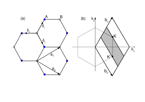
Figure 1: (a) The lattice unit vectors $\mathbf{a}_{1}$ and $\mathbf{a}_{2}$ in a unit cell of a hexagonal lattice of graphene. (b) The corresponding Brillouin zone, and the Dirac cones are located at the $\mathbf{K}$ and $\mathbf{K}^{\prime}$ points. The shadowed area indicates the region with non-zero electric polarization.

Spinless graphene as a two-dimensional topological Dirac semimetal - Since the spin-orbit coupling in graphene is tiny Yao07prb , we assume the spin degeneracy of electrons here. The energy dispersions of electrons in graphene have been investigated extensivelyNeto09rmp ; Wakabayashi10stam . To diagonalize the tight-biding model for graphene, a basis of two-component “spinors” of Bloch states constructed on the two sublattices $\mathbf{A}$ and $\mathbf{B}$ is introduced Neto09rmp . Let $\delta_{1}$, $\delta_{2}$ and $\delta_{3}$ be the displacements from a B site to its three nearest-neighbor A sites as shown in Fig. 1(a). The lattice vectors are chosen to be $\mathbf{a}_{1}=\sqrt{3}a(\frac{\sqrt{3}}{2},\frac{1}{2})$ and $\mathbf{a}_{2}=\sqrt{3}a(\frac{\sqrt{3}}{2},-\frac{1}{2})$. The corresponding reciprocal lattice vectors are $\mathbf{b}_{1}=\frac{4\pi}{3a}(\frac{1}{2},\frac{\sqrt{3}}{2})$ and $\mathbf{b}_{2}=\frac{4\pi}{3a}(\frac{1}{2},-\frac{\sqrt{3}}{2})$. In this representation the Hamiltonian becomes

$$H=-t\sum_{\mathbf{k}}\left(\begin{array}[]{cc}0&\phi(\mathbf{k})\\ \phi^{*}(\mathbf{k})&0\end{array}\right),$$ (1)

where $\sigma_{i}$ are the Pauli matrices and $\phi(\mathbf{k})=\sum_{n=1}^{3}e^{i\mathbf{k}\cdot(\delta_{n}-\delta_{1})}$. The energy band dispersions are obtained as,

$$E_{s}=-st\left|\phi(\mathbf{k})\right|,$$ (2)

where $s=\pm$. The two bands touch at the points of $\mathbf{K}=(\frac{2\pi}{3a},\frac{2\pi}{3\sqrt{3}a})=\frac{2}{3}\mathbf{b}_{1}+\frac{1}{3}\mathbf{b}_{2}$ and $\mathbf{K}^{\prime}=(\frac{2\pi}{3a},-\frac{2\pi}{3\sqrt{3}a})=\frac{1}{3}\mathbf{b}_{1}+\frac{2}{3}\mathbf{b}_{2}$ in the Brillouin zone formed by the reciprocal lattice vectors $\mathbf{b}_{1}$ and $\mathbf{b}_{2}$ as shown in Fig. 1(b), and the dispersions become linear in $k$ approximately measured from the two points. Thus two Dirac cones are formed around $\mathbf{K}$ and $\mathbf{K}^{\prime}$. The density of states is linear in energy $E$ near the two Dirac points, which is a key feature of a semimetal. The vector connecting $\mathbf{K}$ and $\mathbf{K}^{\prime}$ is along $\delta\mathbf{K}=\mathbf{K}-\mathbf{K}^{\prime}=\frac{1}{3}\left(\mathbf{b}_{1}-\mathbf{b}_{2}\right)$. To explore the topological properties of the two Dirac cones, we take $\mathbf{k}=k_{1}\mathbf{b}_{1}+k_{2}\mathbf{b}_{2}$ and consider a specific direction by taking a specific value of $k_{1}$ (or $k_{2}$ ) as a constant, and the model is reduced to one-dimensional along the $\mathbf{b}_{2}$ (or $\mathbf{b}_{1}$) direction. When $k_{1}$ is away from the Dirac points, i.e., $k_{1}\neq 1/3$ and $2/3$, the reduced one-dimensional system always possesses a finite band gap. This gap will close and re-open when $k_{1}$ is sweeping over one Dirac point, which indicates that a topological phase transition may occur in the process.

Ryu and Hatsugai Ryu02prl first realized that zero energy modes in the zigzag ribbon of graphene are closely associated to a hidden chiral symmetry for a reduced one-dimensional Hamiltonian in a parameter space. Denote the eigenstates of $H$ by $\left|\phi_{s}\left(k_{x},k_{y}\right)\right\rangle=\frac{1}{\sqrt{2}}\left(1,s\phi(\mathbf{k})/\left|\phi(\mathbf{k})\right|\right)^{T}$with the eigenvalue $E_{s}(\mathbf{k})$ in Eq. (2). In reduced one-dimensional momentum space, e.g., keeping $k_{1}$ constant, the electric polarization for the reduced one-dimensional bands is defined as Xiao10rmp ; Kingsmith93prb

$$P_{s}=-\frac{e\sqrt{3}a}{2\pi}\oint_{C}dk_{2}\left\langle\phi_{s}(k_{1},k_{2})\right|(i\partial_{k_{2}})\left|\phi_{s}(k_{1},k_{2})\right\rangle.$$ (3)

The electric polarization has its topological origin, and is quantized to be $P_{s}=e\nu_{s}\sqrt{3}a$ where the integer $\nu_{s}=0$ or 1/2 with modulo 1 appears as a topological invariant for quantum transport. It is found that $P_{s}=se\sqrt{3}a/2$ for $1/3<k_{1}<2/3$, and $P_{s}=0$ otherwise. Thus the one-dimensional system is topologically nontrivial when $1/3\leq k_{1}<2/3$. Therefore a spinless graphene is a two-dimensional topological Dirac semimetal characterized by a topological invariant, which is very similar to the three-dimensional Weyl semimetal where a k-dependent Chern number is defined Hosur13Physique . According to the bulk-boundary correspondence, there exists a pair of end modes near the two ends of an open and topological nontrivial chain, and the energy of the end states should be zero due to the chiral symmetry Ryu02prl , just as the end modes in the Su-Schrieffer-Heeger model Shen12book . Correspondingly, the open boundary parallel with the vector $\mathbf{b}_{1}$ (or $\mathbf{b}_{2}$) is the zigzag boundary of the lattice. Each $k_{1}$ in the shadow regime will have a pair of zero energy modes near two edges according to the the bulk-edge correspondence and the particle-hole symmetry in Eq. (1), and a flat band is formed for a zigzag boundary of the graphene lattice. This demonstrates that the famous flat band of graphene with a zigzag boundary condition has its topological origin related to the non-zero electric polarization or topological invariant, just as the Fermi arc in three-dimensional Weyl semimetals Lu15Weyl-shortrange . Unlike that a magnetic monopole is located at a three-dimensional Weyl node, a well-defined $\pi$ Berry phase exists around the Dirac point in two dimensions Suzuura02prl ; Mikitik99prl ; Shen04prb .

Chiral anomaly - It is well known that the chiral charge conservation may be violated for Weyl fermions in three dimensions. Nielsen and Ninomiya Nielsen83plb proposed to simulate the chiral anomaly in one-dimensional chiral bands by using the lowest Landau band of a three-dimensional semimetal in the presence of a magnetic field. Applying an external electric field along the magnetic field will drive electrons flowing from one node to another one, which leads to the so-called Adler-Bell-Jackiw chiral anomaly Adler69pr ; Bell69Jackiw . Consequently, it is expected that the longitudinal magnetoresistivity becomes extremely strong, and negative Nielsen83plb . If the electric field is normal to the magnetic field, the anomaly will disappear. Recently, thanks to the discovery of a number of realistic materials of topological semimetal Xu15sci-TaAs ; Lv15prx , there is growing passion on their electronic transport and signatures of the chiral anomaly Xiong15sci ; ZhangCL16nc ; LiH16nc ; LiQ-16np . Inspired by the advances in three-dimensional Weyl semimetals, it becomes an appealing issue whether or not there also exists the chiral anomaly or its signature in two-dimensional Dirac semimetal or graphene Young15prl . A perpendicular magnetic field can induce discrete Landau bands, but it is always perpendicular to the electric field or electric current in graphene, and an in-plane magnetic field cannot produce Landau bands. Thus it is obvious that there is no chiral anomaly in graphene in the presence of both magnetic and electric fields, opposite to the three-dimensional case. However early works on quasi-one-dimensional graphene nanoribbon has shown that they may support the formation of one-dimensional chiral bands due to the finite-size effect of quantum confinement Peres06prb .

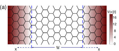
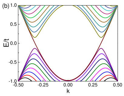
Figure 2: (a) Schematic of a carrier-guiding graphene sheet encapsulated by two confining gates or potentials along the zigzag direction. The shadow area means a confining potential $V(x)$ is added, say $V(x)=V_{0}\left|x\right|$ where $x$ is the position measured from the potential boundary, i.e., the dashed lines. The potential is zero in the white regime. (b) The energy band dispersions near two Dirac points. $k$ is the wave vector. The parameters are $N=20$ , $V_{0}=\frac{3t}{a}$, and $a_{0}=\sqrt{3}a$.

Consider a monolayer graphene sheet encapsulated by two confining gates along the zigzag direction to realize the quasi-one-dimensional ballistic channels as shown in Fig. 2. The width of the free channel is $W=(\frac{3}{2}N-1)a$, where $N\geq 2$ is the site number of one sublattice along the unit vector. Without loss of generality, a confining potential is taken to be $V(x)=V_{0}\left|x\right|$ where $x$ is the position measured away from the dashed line or the potential boundary or as shown in Fig. 2(a). $V_{0}$ represents the strength of the confining potential. It is worth of emphasizing that the finial result in this paper is not so sensitive to the form of the confining potential. Due to the effect of quantum confinement, the energy dispersion evolves into a set of one-dimensional chiral bands. Modes $n=1,2,3,\cdots,N$ lie in the right valley whereas modes $n=-1,-2,\cdots,-N$ lie in the left valley. At each valley, the energy spacing for different non-zero energy bands is approximately $\triangle=\frac{3\pi}{2}\frac{ta}{W}$, and the gap between conduction band and valence band is about $3\Delta$. Within the band gap, the zeroth mode, $n=0$, with nearly linear dispersion crossing two the Dirac points at $k=\pm 1/3$ with opposite velocities, $v=\pm\frac{3}{2}ta/\hbar$. Take the periodic boundary condition along the vertical direction. The energy band dispersion is shown in Fig. 2b. The energy dispersions are split into a series of energy bands due to the confining effect of the potential, which are very similar to the Landau bands induced by an external magnetic field in graphene Rammal85jp , and also those in topological Weyl semimetals Lu15Weyl-shortrange . It is noted that the shape and position of $n=0$ mode depends on the strength of potential. When $V_{0}\rightarrow\infty$, it is similar to a zigzag nanoribbon, in which the modes will be flattened Peres06prb ; Rycerz07np .

In the absence of an external electric field, if the Fermi level is near $E_{F}=0$, the effective velocities at the points of the Fermi level are opposite to each other, the right one is positive and the left one is negative, indicating the formation of chiral states. Applying an external electric field will drive electrons flowing from one valley to the other. The change rate of the density of charge carriers at one valley $s$($=\pm$) is $\frac{dn_{s}}{dt}=\frac{s}{2\pi W}\frac{2\pi}{a_{0}}\frac{dk}{dt}$, and $\frac{d}{dt}\left(k\frac{2\pi}{a_{0}}\right)=\frac{eE}{\hbar}$. Thus the change rate at each valley is

$$\frac{dn_{s}}{dt}=s\frac{e}{h}\frac{E}{W},$$ (4)

indicating the violation of the charge conservation at each valley, although the total charges of the whole system is conserved, $d(n_{+}+n_{-})/dt=0$. Thus the chiral anomaly of two-dimensional Dirac fermions can also be realized, as an analog of three-dimensional Weyl fermions in parallel electric and magnetic fields Nielsen83plb . For three-dimensional Weyl fermions, the changing rate of density at each valley is proportional to $\mathbf{B}\cdot\mathbf{E}$ ($\mathbf{B}$ is the magnetic field and E is the electric field), and the chiral anomaly disappears when the electric field is normal to the magnetic field. Here the anisotropy of chiral anomaly in graphene is determined by the orientation of the confining potential. If the confining potential is along the armchair direction $\mathbf{a}_{0}$, i.e., along the direction of $\mathbf{a}_{1}+\mathbf{a}_{2}$, the chiral band crossing the conduction and valence bands may disappear, and consequently, so does the chiral anomaly. For a specific orientation of confining potential between the armchair and zigzag orientation, $\mathbf{a}=\cos\theta\mathbf{a}_{2}+\sin\theta\mathbf{a}_{0}$, where $\theta$ varies from 0 to $\pi/2$, the change rate will be modified by a factor $\cos\theta$ , which approaches zero when $\theta=\pi/2$.

It is noted that the ferromagnetism may appear along the zigzag edge of a graphene nanoribbon Son-Nature-06 ; Tao-11np . Due to the fact that the dispersions still connect two valleys, the current mechanism of the chiral anomaly will survive when the Fermi level crosses the the edge dispersions.

Signature of chiral anomaly - Now we come to explore the measurable signature of chiral anomaly in graphene. It is known that the chiral anomaly of Weyl fermions generates the chiral magnetic effect Vilenkin80prd ; Nielsen83plb ; Fukushima08prd . Its magnetoconductivity is positive and quadratic in magnetic field B LiQ-16np . As the change rate of Dirac fermions at each valley in graphene is proportional to $1/W$, a finite-size conductivity is expected to reveal a signature of chiral anomaly for Dirac fermions in graphene. Consider the relation between the density of charge carriers $n_{\pm}$ and the chemical potential $\mu_{\pm}$, $n_{\pm}=\frac{1}{4\pi}\frac{\mu_{\pm}^{2}}{\left(v_{F}\hbar\right)^{2}}$ at each valley. Without loss of generality, assume the chemical potentials are positive, i.e., in the electron doped case. In the presence of an electric field, electrons will flow from the right valley to the left valley, and cause a difference of chemical potentials, $\delta\mu=\mu_{+}-\mu_{-}.$ However, the process will be balanced by the inter-valley scattering between the left and right moving electrons. Consider the lateral diffusive regime where the mean free path is shorter than the width, and denote the inter-valley scattering time by $\tau_{v}$. The equation for the chiral anomaly is reduced to

$$\frac{d(n_{+}-n_{-})}{dt}=2\frac{eE}{hW}-\frac{n_{+}-n_{-}}{\tau_{v}}.$$ (5)

In a steady state, the solution to the equation is $n_{+}-n_{-}=2\frac{eE}{hW}\tau_{v}$. Thus the difference of the chemical potentials at two valley is $\delta\mu=\frac{2\pi\left(v_{F}\hbar\right)^{2}}{\mu}\frac{2eE}{hW}\tau_{v}$ (assume $\mu\neq 0$)note-1 . As the Fermi levels at two valleys are different, and the change rate of electrons is finite due to the chiral anomaly, the energy cost for transferring the electrons from one valley to the other is simply the product of the change rate of electrons at each valley and the energy difference between the two valleys. This energy must be extracted from the Joule’s heating in the presence of a charge current, and the energy balance gives $jE=2\frac{eE}{hW}\delta\mu$ Nielsen83plb , where the factor 2 comes from the spin degeneracy in graphene. Thus the solution to the current is

$$j=\frac{2e}{hW}\delta\mu=2\frac{e^{2}v_{F}^{2}\tau_{v}}{\pi\mu W^{2}}E$$ (6)

Consequently the conductivity correction due to the chiral anomaly is $\sigma_{W}=\frac{2e^{2}v_{F}^{2}\tau_{v}}{\pi\mu W^{2}}$, which is proportional to $1/W^{2}$. It is an anomalous behavior that the conductivity correction increases with decreasing the width in $W^{2}$. The inter-valley scattering time $\tau_{v}$ depends on the scattering mechanism. If the scattering potential is short ranged of the form $V=v_{0}\delta(\mathbf{r})$, the inter-valley scattering time is given by $\tau_{v}\sim\frac{4v_{F}}{n_{i}v_{0}^{2}}\frac{1}{\left|\delta\mathbf{K}\right|}$ where $n_{i}$ is the impurity density Shon-98jpsj . Thus $\sigma_{W}$ is proportional to the square root of the density of charge carriers, $\sigma_{W}\propto 1/\sqrt{n}$. To estimate the order of the finite size correction, we take $\mu=\tilde{\mu}$eV, $W=\tilde{W}$nm, $l=v_{F}\tau_{v}=\tilde{l}$nm, and $v_{F}=10^{6}\mathrm{m/s}$, and have $\sigma_{W}\simeq 2.63\frac{\tilde{l}}{\tilde{\mu}\tilde{W}^{2}}\frac{e^{2}}{h}$ . $\tilde{\mu}\sim 0.1$ for the charge density $n\sim 10^{12}/\mathrm{cm}^{2}$. The intervalley scattering length is much longer than the mean free path in graphene Shon-98jpsj ; Morpurgo-06prl . Thus for a sample with scattering length of several tens of nanometer, the correction is measurable for $W$ up to several tens or even hundred of nanometers. The conventional Drude conductivity of graphene $\sigma_{0}$ was found to proportional to the density of charge carriers, $n$, while reaches at a minimal conductivity at the charge neutral point Shon-98jpsj ; Nomura-07prl ; Cheianov-06prl ; Adam-07pnas . The conductivity is always of the order of $e^{2}/h$ and has a weak dependence on size Lewenkopf-08prb ; Neto09rmp . The quantized conductance in steps of $4e^{2}/h$ has been measured in a graphene nanoribbon Kim-16np . For wires or ribbons without boundary modes, the conductivity usually has a negative correction due to excess scattering from the boundary which is inversely proportional to $W$. In the presence of a boundary mode, the correction can become positive, but still goes inversely with $W$. However, the anomalous correction here is always positive and goes inversely with the square of $W$.

Summary - In short, we propose that the chiral anomaly of two-dimensional Dirac fermions can be realized in a quasi-one-dimensional monolayer graphene, and its signature can be detected by measuring the finite-size conductivity. It is necessary to emphasize that we consider the laterally diffusive regime where the mean free path is shorter than the width. When the mean free path is much larger than the width $W$, the story will be very different. It is believed that this property is associated with the chiral symmetry of the Dirac fermions in the reduced one-dimensional momentum space, and the formation of chiral currents of the system. Chiral anomaly is a purely quantum mechanical effect for Weyl fermions. It is widely accepted that the positive magnetoconductivity or negative magnetoresistance in topological Weyl semimetals is a signature of chiral anomaly. The anomalous finite-size conductivity in graphene may provide an alternative way to detect this quantum mechanical effect in solid.

This work was supported by the Research Grant Council, University Grants Committee, Hong Kong under Grant No. 17304414 and HKU3/CRF/13G. SQ would like to thank Di Xiao, Jian Li, Hai-Zhou Lu and Jian-Hui Zhou for helpful discussions. This research is conducted in part using the HKU ITS research computing facilities that are supported in part by the Hong Kong UGC Special Equipment Grant (SEG HKU09).

References

- (1) A. H. Castro Neto, F. Guinea, N. M. R. Peres, K. S. Novoselov, and A. K. Geim, Rev. Mod. Phys. 81, 109 (2009).
- (2) G. P. Mikitik and Y. V. Sharlai, Phys. Rev. Lett. 82, 2147 (1999).
- (3) H. Suzuura and T. Ando, Phys. Rev. Lett. 89, 266603 (2002).
- (4) S. Q. Shen, Phys. Rev. B 70, 081311(R) (2004).
- (5) S. M. Young and C. L. Kane, Phys. Rev. Lett. 115, 126803 (2015).
- (6) Y. B. Zhang, Y. W. Tan, H. L. Stormer, and P. Kim, Nature 438, 201 (2005).
- (7) K. S. Novoselov, A. K. Geim, S. V. Morozov, D. Jiang, M. I. Katsnelson, I. V. Grigorieva, S. V. Dubonos, and A. A. Firsov, Nature 438, 197 (2005).
- (8) M. I. Katsnelson, K. S. Novoselov, and A. K. Geim, Nat. Phys. 2, 620 (2006).
- (9) D. Xiao, G.-B. Liu, W. Feng, X. Xu, and W. Yao, Phys. Rev. Lett. 108, 196802 (2012).
- (10) A. Rycerz, J. Tworzydlo, and C. W. J. Beenakker, Nat. Phys. 3, 172 (2007).
- (11) G. E. Volovik, The Universe in a Helium Droplet (Clarendon Press, Oxford, 2003).
- (12) X. Wan, A. M. Turner, A. Vishwanath, and S. Y. Savrasov, Phys. Rev. B 83, 205101 (2011).
- (13) G. Xu, H. M. Weng, Z. J. Wang, X. Dai, and Z. Fang, Phys. Rev. Lett. 107, 186806 (2011).
- (14) A. A. Burkov and L. Balents, Phys. Rev. Lett. 107, 127205 (2011).
- (15) K. Y. Yang, Y. M. Lu, and Y. Ran, Phys. Rev. B 84, 075129 (2011).
- (16) S. Y. Xu, I. Belopolski, N. Alidoust, M. Neupane, G. Bian, C. L. Zhang, R. Sankar, G. Q. Chang, Z. J. Yuan, C. C. Lee, et al., Science 349, 613 (2015).
- (17) B. Q. Lv, H. M. Weng, B. B. Fu, X. P. Wang, H. Miao, J. Ma, P. Richard, X. C. Huang, L. X. Zhao, G. F. Chen, et al., Phys. Rev. X 5, 031013 (2015).
- (18) C. L. Zhang, S.-Y. Xu, I. Belopolski, Z. Yuan, Z. Lin, B. Tong, G. Bian, N. Alidoust, C. C. Lee, S. M. Huang, et al., Nat Commun. 7, 10735 (2016).
- (19) S. Ryu and Y. Hatsugai, Phys. Rev. Lett. 89, 077002 (2002).
- (20) S. L. Adler, Phys. Rev. 177, 2426 (1969).
- (21) J. S. Bell and R. Jackiw, Il Nuovo Cimento A 60, 47 (1969).
- (22) Y. Yao, F. Ye, X. L. Qi, S. C. Zhang, and Z. Fang, Phys. Rev. B 75, 041401 (2007).
- (23) K. Wakabayashi, K. ichi Sasaki, T. Nakanishi, and T. Enoki, Science and Technology of Advanced Materials 11, 054504 (2010).
- (24) D. Xiao, M. C. Chang, and Q. Niu, Rev. Mod. Phys. 82, 1959 (2010).
- (25) R. D. King-Smith and D. Vanderbilt, Phys. Rev. B 47, 1651 (1993).
- (26) P. Hosur and X. Qi, C. R. Physique 14, 857 (2013).
- (27) S. Q. Shen, Topological Insulators (Springer-Verlag, Berlin Heidelberg, 2012).
- (28) H. Z. Lu, S. B. Zhang, and S. Q. Shen, Phys. Rev. B 92, 045203 (2015).
- (29) H. B. Nielsen and M. Ninomiya, Physics Letters B 130, 389 (1983).
- (30) J. Xiong, S. K. Kushwaha, T. Liang, J. W. Krizan, M. Hirschberger, W. Wang, R. J. Cava, and N. P. Ong, Science 10, 1126 (2015).
- (31) H. Li, H. He, H.-Z. Lu, H. Zhang, H. Liu, R. Ma, Z. Fan, S. Q. Shen, and J. Wang, Nat Commun. 7, 10301 (2016).
- (32) Q. Li, D. E. Kharzeev, C. Zhang, Y. Huang, I. Pletikosic, A. V. Fedorov, R. D. Zhong, J. A. Schneeloch, G. D. Gu, and T. Valla, Nat. Phys. 12, 550 (2016).
- (33) N. M. R. Peres, A. H. Castro Neto, and F. Guinea, Phys. Rev. B 73, 195411 (2006).
- (34) Y. W. Son, M. L. Cohen, and S. G. Louie, Nature 444, 347 (2006).
- (35) C. Tao, et al., Nat. Phys. 7, 616 (2011)).
- (36) R. Rammal, J. Phys. France 46, 1345 (1985).
- (37) A. Vilenkin, Phys. Rev. D 22, 3080 (1980).
- (38) For , , and the charge current is . However at this point other effects such as disorders or fluctuations become dominant to produce a minimal conductivity.
- (39) K. Fukushima, D. Kharzeev and H. Warringa, Phys. Rev. D 78, 074033 (2008).
- (40) N. H. Shon and T. Ando, J. Phys. Soc. Jpn. 67, 2421 (1998).
- (41) A. F. Morpurgo and F. Guinea, Phys. Rev. Lett. 97, 196804 (2006).
- (42) K. Nomura and A. H. MacDonald, Phys. Rev. Lett. 98, 076602 (2007).
- (43) V. V. Cheianov and V. I. Falko, Phys. Rev. Lett. 97, 226801 (2006).
- (44) S. Adam, E. H. Hwang, V. M. Galitski and S. Das Sarma, Proc. Natl. Acad. Sci. USA, 104, 18392 (2007).
- (45) C. H. Lewenkopf, E. R. Mucciolo, and A. H. Castro Neto, Phys. Rev. B 77, 081410 (2008).
- (46) M. Kim, J. H. Choi, S. H. Lee, K. Watanabe, T. Taniguchi, S. H. Jhi and H. J. Lee, Nat. Phys. 12, 1022 (2016).