Beyond Whittle: Nonparametric correction of a parametric likelihood with a focus on Bayesian time series analysis

Abstract

Abstract. The Whittle likelihood is widely used for Bayesian nonparametric estimation of the spectral density of stationary time series. However, the loss of efficiency for non-Gaussian time series can be substantial. On the other hand, parametric methods are more powerful if the model is well-specified, but may fail entirely otherwise. Therefore, we suggest a nonparametric correction of a parametric likelihood taking advantage of the efficiency of parametric models while mitigating sensitivities through a nonparametric amendment. Using a Bernstein-Dirichlet prior for the nonparametric spectral correction, we show posterior consistency and illustrate the performance of our procedure in a simulation study and with LIGO gravitational wave data.

1 Introduction

Statistical models can be broadly classified into parametric and nonparametric models. Parametric models, indexed by a finite dimensional set of parameters, are focused, easy to analyse and have the big advantage that when correctly specified, they will be very efficient and powerful. However, they can be sensitive to misspecifications and even mild deviations of the data from the assumed parametric model can lead to unreliabilities of inference procedures. Nonparametric models, on the other hand, do not rely on data belonging to any particular family of distributions. As they make fewer assumptions, their applicability is much wider than that of corresponding parametric methods. However, this generally comes at the cost of reduced efficiency compared to parametric models.

Standard time series literature is dominated by parametric models like autoregressive integrated moving average models (Box et al., 2013), the more recent autoregressive conditional heteroskedasticity models for time-varying volatility (Engle, 1982; Bollerslev, 1986), state-space (Durbin and Koopman, 2012), and Markov switching models (Bauwens et al., 2000). In particular, Bayesian time series analysis (Steel, 2008) is inherently parametric in that a completely specified likelihood function is needed. Nonetheless, the use of nonparametric techniques has a long tradition in time series analysis. (Schuster, 1898) introduced the periodogram which may be regarded as the origin of spectral analysis and a classical nonparametric tool for time series analysis (Härdle et al., 1997). Frequentist time series analyses especially use nonparametric methods (Fan and Yao, 2002; Wasserman, 2006) including a variety of bootstrap methods, computer-intensive resampling techniques initially introduced for independent data, that have been taylored to and specifically developed for time series (Härdle et al., 2003; Kreiss and Lahiri, 2012; Kreiss and Paparoditis, 2011). An important class of nonparametric methods is based on frequency domain techniques, most prominently smoothing the periodogram. These include a variety of frequency domain bootstrap methods strongly related to the Whittle likelihood (Hurvich and Zeger, 1987; Franke and Härdle, 1992; Kirch and Politis, 2011; Kirch, 2007; Kim and Nordman, 2013) and found important applications in a variety of disciplines (Hidalgo, 2008; Costa et al., 2013; Emmanoulopoulos et al., 2013).

Despite the fact that nonparametric Bayesian inference has been rapidly expanding over the last decade, as reviewed by Hjort et al. (2010), Müller and Mitra (2013), and Walker (2013), only very few nonparametric Bayesian approaches to time series analysis have been developed. Most notably, Carter and Kohn (1997), Gangopadhyay et al. (1999), Liseo et al. (2001), Choudhuri et al. (2004a), Hermansen (2008), and Chopin et al. (2013) used the Whittle likelihood Whittle (1957) for Bayesian modelling of the spectral density as the main nonparametric characteristic of stationary time series. The Whittle likelihood is an approximation of the true likelihood. It is exact only for Gaussian white noise. However, even for non-Gaussian stationary time series which are not completely specified by their first and second-order structure, the Whittle likelihood results in asymptotically correct statistical inference in many situations. As shown in Contreras-Cristán et al. (2006), the loss of efficiency of the nonparametric approach using the Whittle likelihood can be substantial even in the Gaussian case for small samples if the autocorrelation of the Gaussian process is high.

On the other hand, parametric methods are more powerful than nonparametric methods if the observed time series is close to the considered model class but fail if the model is misspecified. To exploit the advantages of both parametric and nonparametric approaches, the autoregressive-aided periodogram bootstrap has been developed by Kreiss and Paparoditis (2003) within the frequentist bootstrap world of time series analysis. It fits a parametric working model to generate periodogram ordinates that mimic the essential features of the data and the weak dependence structure of the periodogram while a nonparametric correction is used to capture features not represented by the parametric fit. This has been extended in various ways (see Jentsch and Kreiss (2010); Jentsch et al. (2012); Kreiss and Paparoditis (2012)). Its main underlying idea is a nonparametric correction of a parametric likelihood approximation. The parametric model is used as a proxy for rough shape of the autocorrelation structure as well as the dependency structure between periodogram ordinates. Sensitivities with respect to the spectral density are mitigated through a nonparametric amendment. We propose to use a similar nonparametrically corrected likelihood approximation as a pseudo-likelihood in the Bayesian framework to compute the pseudo-posterior distribution of the power spectral density (PSD) and other parameters in time series models. This will yield a pseudo-likelihood that generalises the widely used Whittle likelihood which, as we will show, can be regarded as a special case of a nonparametrically corrected likelihood under the Gaussian i.i.d. working model. Software implementing the methodology is available in the R package beyondWhittle, which is available on the Comprehensive R Archive Network (CRAN), see Meier et al. (2017).

The paper is structured as follows: In Chapter 2, we briefly revisit the Whittle likelihood and demonstrate that it is a nonparametrically corrected likelihood, namely that of a Gaussian i.i.d. working model. Then, we extend this nonparametric correction to a general parametric working model. The corresponding pseudo-likelihood turns out to be equal to the true likelihood if the parametric working model is correctly specified but also still yields asymptotically unbiased periodogram ordinates if it is not correctly specified. In Chapter 3, we propose a Bayesian nonparametric approach to estimating the spectral density using the pseudo-posterior distribution induced by the corrected likelihood of a fixed parametric model. We describe the Gibbs sampling implementation for sampling from the pseudo-posterior. This nonparametric approach is based on the Bernstein polynomial prior of Petrone (1999) and used to estimate the spectral density via the Whittle likelihood in Choudhuri et al. (2004a). We show posterior consistency of this approach and discuss how to incorporate the parametric working model in the Bayesian inference procedure. Chapter 4 gives results from a simulation study, including case studies of sunspot data, and gravitational wave data from the sixth science run of the Laser Interferometric Gravitational Wave Observatory (LIGO). This is followed by discussion in Chapter 5, which summarises the findings and points to directions for future work. The proofs, the details about the Bayesian autoregressive sampler as well as some additional simulation results are deferred to the Appendices A – C.

2 Likelihood approximation for time series

While the likelihood of a mean zero Gaussian time series is completely characterised by its autocovariance function, its use for nonparametric frequentist inference is limited as it requires estimation in the space of positive definite covariance functions. Similarly for nonparametric Bayesian inference, it necessitates the specification of a prior on positive definite autocovariance functions which is a formidable task. A quick fix is to use parametric models such as ARMA models with data-dependent order selection, but these methods tend to produce biased results when the ARMA approximation to the underlying time series is poor. A preferable nonparametric route is to exploit the correspondence of the autocovariance function and the spectral density via the Wiener-Khinchin theorem and nonparametrically estimate the spectral density. To this end, Whittle (1957) defined a pseudo-likelihood, known as the Whittle likelihood, that directly depends on the spectral density rather than the autocovariance function and that gives a good approximation to the true Gaussian and certain non-Gaussian likelihoods. In the following subsection we will revisit this approximate likelihood proposed by Whittle (1957), before introducing a semiparametric approach which extends the Whittle likelihood.

2.1 Whittle likelihood revisited

Assume that $\{Z_{t}\colon t=0,1,\ldots\}$ is a real zero mean stationary time series with absolutely summable autocovariance function $\sum_{h\in\mathbb{Z}}|\gamma(h)|<\infty$. Under these assumptions the spectral density of the time series exists and is given by the Fourier transform (FT) of the autocovariance function

$$f(\lambda)=\frac{1}{2\pi}\sum_{k=-\infty}^{\infty}\gamma(k)\exp^{-ik\lambda},\quad 0\leq\lambda\leq 2\pi.$$

Consequently, there is a one-to-one-correspondence between the autocovariance function and the spectral density, and estimation of the spectral density is amenable to smoothing techniques. The idea behind these smoothing techniques is the following observation, which also gives rise to the so-called Whittle approximation of the likelihood of a time series: Consider the periodogram of $\mathbf{Z}_{n}=(Z_{1},\ldots,Z_{n})^{T}$,

$$I_{n}(\lambda)=I_{n,\lambda}(\mathbf{Z}_{n})=\frac{1}{2\pi n}\left|\sum_{t=1}^{n}Z_{t}\exp^{-it\lambda}\right|^{2}.$$

The periodogram is given by the squared modulus of the discrete Fourier coefficients, the Fourier transformed time series evaluated at Fourier frequencies $\lambda_{j}=\frac{2\pi j}{n}$, for $j=0,\ldots,N=\lfloor(n-1)/2\rfloor$. It can be obtained by the following transformation: Define for $j=1,\ldots,N$

$$\mathbf{c}_{j}=\sqrt{2}\Re\mathbf{e}_{j}=\frac{1}{\sqrt{2}}(\mathbf{e}_{j}+\mathbf{e}_{n-j}),\qquad\mathbf{s}_{j}=\sqrt{2}\Im\mathbf{e}_{j}=\frac{1}{i\,\sqrt{2}}(\mathbf{e}_{j}-\mathbf{e}_{n-j}),$$

where

$$\mathbf{e}_{j}=n^{-1/2}(e_{j},e_{j}^{2},\ldots,e_{j}^{n})^{T},\qquad e_{j}=\exp(-2\pi ij/n),\qquad j=0,\ldots,N$$

and for $n$ even, $\mathbf{e}_{n/2}$ is defined analogously. Then,

$$F_{n}=\begin{cases}(\mathbf{e}_{0},\mathbf{c}_{1},\mathbf{s}_{1},\ldots,\mathbf{c}_{N},\mathbf{s}_{N},\mathbf{e}_{n/2})^{T},&n\text{ even},\\ (\mathbf{e}_{0},\mathbf{c}_{1},\mathbf{s}_{1},\ldots,\mathbf{c}_{N},\mathbf{s}_{N})^{T},&n\text{ odd},\end{cases}$$

is an orthonormal $n\times n$ matrix (cf. e.g. Brockwell and Davis (2009), paragraph 10.1). Real- and imaginary parts of the discrete Fourier coefficients are collected in the vector

$${\tilde{\mathbf{Z}}}_{n}:=(\tilde{Z}_{n}(0),\ldots,\tilde{Z}_{n}(n-1))^{T}=F_{n}\mathbf{Z}_{n}$$

and the periodogram can be written as

$$I_{n}(\lambda_{j})=\frac{1}{4\pi}\left(\tilde{Z}_{n}^{2}(2j)+\tilde{Z}^{2}_{n}(2j-1)\right),\quad j=1,\ldots,N,$$

$$I_{n}(\lambda_{0})=\frac{1}{2\pi}\tilde{Z}_{n}^{2}(0),\qquad\text{as well as for }n\text{ even: }I_{n}(\lambda_{n/2})=\frac{1}{2\pi}\tilde{Z}_{n}^{2}(n-1).$$ (1)

It is well known that the periodograms evaluated at two different Fourier frequencies are asymptotically independent and have an asymptotic exponential distribution with mean equal to the spectral density, a statement that remains true for non-Gaussian and even non-linear time series Shao and Wu (2007). Similarly, the Fourier coefficients $\boldsymbol{\tilde{Z}}_{n}$ are asymptotically independent and normally distributed with variances equal to $2\pi$ times the spectral density at the corresponding frequency. This result gives rise to the following Whittle approximation in the frequency domain

$$p_{\widetilde{\mathbf{Z}}_{n}}^{W}(\boldsymbol{\tilde{z}}_{n}|f)\propto\det(D_{n})^{-1/2}\exp\left(-\frac{1}{2}\boldsymbol{\tilde{z}}_{n}^{T}D_{n}^{-1}\boldsymbol{\tilde{z}}_{n}\right)$$ (2)

by the likelihood of a Gaussian vector with diagonal covariance matrix

$$D_{n}:=D_{n}(f):=2\pi\,\begin{cases}\text{diag}(f(0),f(\lambda_{1}),f(\lambda_{1}),\ldots,f(\lambda_{N}),f(\lambda_{N}),f(\lambda_{n/2}))&n\text{ even},\\ \text{diag}(f(0),f(\lambda_{1}),f(\lambda_{1}),\ldots,f(\lambda_{N}),f(\lambda_{N}))&n\text{ odd}.\end{cases}$$ (3)

As explicitly shown in Appendix A, this yields the famous Whittle likelihood in the time domain via the transformation theorem

$$p^{W}_{\mathbf{Z}_{n}=F_{n}^{T}\boldsymbol{\tilde{Z}}_{n}}(\boldsymbol{z}_{n}|f)\propto\exp\left\{-\frac{1}{2}\sum_{j=0}^{n-1}\left(\log f(\lambda_{j})+\frac{I_{n,\lambda_{j}}(\boldsymbol{z}_{n})}{f(\lambda_{j})}\right)\right\}$$ (4)

which provides an approximation of the true likelihood. It is exact only for Gaussian white noise in which case $f(\lambda_{j})=\sigma^{2}/2\pi$. It has the advantage that it depends directly on the spectral density in contrast to the true likelihood that depends on $f$ indirectly via Wiener-Khinchin’s theorem. Sometimes, the summands corresponding to $j=0$ as well as $j=n/2$ (the latter for $n$ even) are omitted in the likelihood approximation. In fact, the term corresponding to $j=0$ contains the sample mean (squared) while the term corresponding to $j=n/2$ gives the alternating sample mean (squared). Both have somewhat different statistical properties and usually need to be considered separately. Furthermore, the first term is exactly zero if the methods are applied to time series that have been centered first, while the last one is approximately zero and asymptotically negligible (refer also Remark 3.2).

The density of $F_{n}^{T}D_{n}^{1/2}F_{n}\mathbf{Z}_{n}$ under the i.i.d. standard Gaussian working model is the Whittle likelihood. It has two potential sources of approximation errors: The first one is the assumption of independence between Fourier coefficients which holds only asymptotically but not exactly for a finite time series, the second one is the Gaussianity assumption. In this paper, we restrict our attention to the first problem, extending the proposed methods to non-Gaussian situations will be a focus of future work. In fact, the independence assumption leads to asymptotically consistent results for Gaussian data. But even for Gaussian data with relatively small sample sizes and relatively strong correlation the loss of efficiency of the nonparametric approach using the Whittle likelihood can be substantial as shown in Contreras-Cristán et al. (2006) or by the simulation results of Kreiss and Paparoditis (2003).

2.2 Nonparametric likelihood correction

The central idea in this work is to extend the Whittle likelihood by proceeding from a certain parametric working model (with mean 0) for $\mathbf{Z}_{n}$ rather than an i.i.d. standard Gaussian working model before making a correction analogous to the Whittle correction in the frequency domain.

To this end, we start with some parametric likelihood in the time domain, such as e.g. obtained from an ARMA-model, that is believed to be a reasonable approximation to the true time series. We denote the spectral density that corresponds to this parametric working model by $f_{\text{param}}(\cdot)$. If the model is misspecified, then this spectral density is also wrong and needs to be corrected to obtain the correct second-order dependence structure. To this end, we define a correction matrix

$$C_{n}=C_{n}(f,f_{\text{param}})=C_{n}(c(\lambda))\qquad\left(c:=\frac{f}{f_{\text{param}}}\right)$$

$$=\begin{cases}\text{diag}\left(\frac{f(\lambda_{0})}{f_{\text{param}}(\lambda_{0})},\frac{f(\lambda_{1})}{f_{\text{param}}(\lambda_{1})},\frac{f(\lambda_{1})}{f_{\text{param}}(\lambda_{1})},\ldots,\frac{f(\lambda_{N})}{f_{\text{param}}(\lambda_{N})},\frac{f(\lambda_{N})}{f_{\text{param}}(\lambda_{N})},\frac{f(\lambda_{n/2})}{f_{\text{param}}(\lambda_{n/2})}\right)&n\text{ even},\\ \text{diag}\left(\frac{f(\lambda_{0})}{f_{\text{param}}(\lambda_{0})},\frac{f(\lambda_{1})}{f_{\text{param}}(\lambda_{1})},\frac{f(\lambda_{1})}{f_{\text{param}}(\lambda_{1})},\ldots,\frac{f(\lambda_{N})}{f_{\text{param}}(\lambda_{N})},\frac{f(\lambda_{N})}{f_{\text{param}}(\lambda_{N})}\right)&n\text{ odd}.\end{cases}$$

This is analogous to the Whittle correction in the previous section as, in particular, $D_{n}=C_{n}(f,f_{\text{ i.i.d.}N(0,1)})$ with $D_{n}$ as in (3). However, the corresponding periodogram ordinates are no longer independent under this likelihood but instead inherit the dependence structure from the original parametric model (see Proposition 2.1 c). Such an approach in a bootstrap context has been proposed and successfully applied by Kreiss and Paparoditis (2003) using an AR($p$) approximation. This concept of a nonparametric correction of a parametric time domain likelihood is illustrated in the schematic diagram:

$$\begin{array}[]{lcl}\underline{\mbox{time domain}}&&\underline{\mbox{frequency domain}}\\ \mathbf{Z}_{n}\sim\text{parametric working model}&\mbox{ }\stackrel{{\scriptstyle\mbox{ $\operatorname{FT}$}}}{{\xrightarrow{\hskip 71.13188pt}}}\mbox{ }&F_{n}\mathbf{Z}_{n}\\ &&{\left\downarrow\vbox to22.76228pt{}\right.\kern-1.2pt}C_{n}(f,f_{\text{param}})\\ F_{n}^{T}C_{n}(f,f_{\text{param}})^{1/2}F_{n}\mathbf{Z}_{n}&\stackrel{{\scriptstyle\mbox{ $\operatorname{FT}^{-1}$}}}{{\xleftarrow{\hskip 71.13188pt}}}&C_{n}(f,f_{\text{param}})^{1/2}F_{n}\mathbf{Z}_{n}\\ \end{array}$$

As a result we obtain the following nonparametrically corrected likelihood function under the parametric working model

$$p_{\text{param}}^{C}(\mathbf{Z}_{n}|f)\propto\det(C_{n})^{-1/2}\;p_{\text{param}}(F_{n}^{T}C_{n}^{-\frac{1}{2}}F_{n}\mathbf{Z}_{n}),$$ (5)

where $p_{\text{param}}$ denotes the parametric likelihood.

Remark 2.1

Parametric models with a multiplicative scale parameter $\sigma\neq 1$ yield the same corrected likelihood as the one with $\sigma=1$ , i.e. if $\sigma\mathbf{Z}_{n}$ is used as working model this leads to the same corrected likelihood for all $\sigma>0$. For instance, if the parametric model is given by i.i.d. $N(0,\sigma^{2})$ random variables with $\sigma^{2}>0$ arbitrary, then the correction also results in the Whittle likelihood (for a proof we refer to Appendix A). Analogously, for linear models $Z_{t}=\sum_{l=-\infty}^{\infty}d_{l}e_{t-l}$, $e_{t}\sim(0,\sigma^{2})$, which includes the class of ARMA-models, the corrected likelihood is independent of $\sigma^{2}$.

We can now prove the following proposition which shows two important things: First, the corrected likelihood is the exact likelihood in case the parametric model is correct. Second, the periodograms associated with this likelihood are asymptotically unbiased for the true spectral density regardless of whether the parametric model is true.

Proposition 2.1

Let $\{Z_{t}\}$ be a real zero mean stationary time series with absolutely summable autocovariance function $\sum_{h\in\mathbb{Z}}|\gamma(h)|<\infty$ and let $f_{\text{param}}(\lambda)\geq\beta>0$ for $0\leq\lambda\leq\pi$ be the spectral density associated with the (mean zero) parametric model used for the correction.

1. If $f=f_{\text{param}}$, then $p_{\text{param}}^{C}=p_{\text{param}}$.

2. The periodogram associated with the corrected likelihood is asymptotically unbiased for the true spectral density, i.e.

   $$\operatorname{E}_{p_{\text{param}}^{C}}I_{n,\lambda_{j}}(\mathbf{Z}_{n}) =\int I_{n,\lambda_{j}}(z_{1},\ldots,z_{n})\,dp_{\text{param}}^{C}(z_{n},\ldots,z_{n})$$

   $${=\frac{f(\lambda_{j})}{f_{\text{param}}(\lambda_{j})}\operatorname{E}_{p_{\text{param}}}I_{n,\lambda_{j}}(\mathbf{Z}_{n})}=f(\lambda_{j})+o(1),$$

   where the convergence is uniform in $j=0,\ldots,\lfloor(n-1)/2\rfloor$. Furthermore,

   $$\operatorname{Cov}_{p_{\text{param}}^{C}}(I_{n,\lambda_{l}}(\mathbf{Z}_{n}),I_{n,\lambda_{k}}(\mathbf{Z}_{n}))=\frac{f(\lambda_{l})f(\lambda_{k})}{f_{\text{param}}(\lambda_{l})\,f_{\text{param}}(\lambda_{k})}\,\operatorname{Cov}_{p_{\text{param}}}(I_{n,\lambda_{l}}(\mathbf{Z}_{n}),I_{n,\lambda_{k}}(\mathbf{Z}_{n})).$$

The proof shows that the vector of periodograms under the corrected likelihood has exactly the same distributional properties as the vector of the periodograms under the parametric likelihood multiplied with $f(\cdot)/f_{\text{param}}(\cdot)$. Hence, asymptotic properties as the ones derived in Theorem 10.3.2 in Brockwell and Davis (2009) carry over with the appropriate multiplicative correction.

In the remainder of the paper we describe how to make use of this nonparametric correction in a Bayesian set-up.

3 Bayesian semiparametric approach to time series analysis

To illustrate the Bayesian semiparametric approach and how to sample from the pseudo-posterior distribution, in the following we restrict our attention to an AR($p$) model as our parametric working model for the time series, i.e. $Z_{i}=\sum_{l=1}^{p}a_{l}Z_{i-l}+\epsilon_{i}$, where $\{\epsilon_{i}\}$ are i.i.d. N($0,1)$ random variables with density denoted by $\varphi(\cdot)$. Note that without loss of generality, $\sigma^{2}=1$, cf. Remark 2.1. This yields the parametric likelihood of our working model, depending on the order $p\geq 0$ and on the coefficients $\mathbf{a}=(a_{1},...,a_{p})$:

$$p_{\text{param}}(\mathbf{Z}_{n}|\mathbf{a})\propto p_{\text{param}}(\mathbf{Z}_{p}|\mathbf{a})\prod_{i=p+1}^{n}\varphi\left(Z_{i}-\sum_{l=1}^{p}a_{l}Z_{i-l}\right)$$ (6)

with spectral density

$$f_{\text{param}}(\lambda;\mathbf{a})=\frac{1}{2\pi}\left|1-\sum_{l=1}^{p}a_{l}e^{-il\lambda}\right|^{-2}.$$ (7)

We assume the time series to be stationary and causal a priori. Thus, $\mathbf{a}$ is restricted such that $\phi(z):=1-a_{1}z-...-a_{p}z^{p}$ has no zeros inside the closed unit disc, c.f. Theorem 3.1.1. in Brockwell and Davis (2009). For now, we assume that the parameters $(p,\mathbf{a})$ of the parametric working model are fixed (and in practice set to Bayesian point estimates obtained from a preceding parametric estimation step). An extension to combine the estimation of the parametric model with the nonparametric correction will be detailed later in Section 3.4.

3.1 Nonparametric prior for spectral density inference

For a Bayesian analysis using either the Whittle or nonparametrically corrected likelihood, we need to specify a nonparametric prior distribution for the spectral density. Here we employ the approach by Choudhuri et al. (2004a) which is essentially based on the Bernstein polynomial prior of Petrone (1999) as a nonparametric prior for a probability density on the unit interval. We briefly describe the prior specification and refer to Choudhuri et al. (2004a) for further details.

In contrast to the approach in Choudhuri et al. (2004a), we do not specify a nonparametric prior distribution for the spectral density $f(\cdot)$, but for a pre-whitened version thereof, incorporating the spectral density of the parametric working model into the estimation. To elaborate, for $0\leq\eta\leq 1$, consider the eta-damped correction function

$$c_{\eta}(\lambda)=c_{\eta}(\lambda;{\mathbf{a}}):=f(\lambda)/f_{\text{param}}(\lambda;{\mathbf{a}})^{\eta}.$$ (8)

This corresponds to a reparametrization of the likelihood (5) by replacing $C_{n}=C_{n}(c(\lambda))$ with $C_{n}=C_{n}(c_{\eta}(\lambda;{\mathbf{a}})f_{\text{param}}(\lambda;{\mathbf{a}})^{\eta-1})$.

Remark 3.1

The parameter $\eta$ models the confidence in the parametric model: If $\eta$ is close to $1$ and the model is well-specified, then $c_{\eta}(\cdot)$ will be much smoother than the original spectral density, since $f_{\text{param}}(\cdot)$ already captures the prominent spectral peaks of the data very well. As a consequence, nonparametric estimation of $c_{\eta}(\cdot)$ should involve less effort than nonparametric estimation of $f(\cdot)$ itself. This remains true in the misspecified case, as long as the parametric model does describe the essential features of the data sufficiently well in the sense that it captures at least the more prominent peaks. However, it is possible that the parametric model introduces erroneous spectral peaks if the model is misspecified. In that case, $\eta$ close to zero ensures a damping of the model misspecification, such that nonparametric estimation of $c_{\eta}(\cdot)$ should involve less effort than nonparametric estimation of $f(\cdot)/f_{\text{param}}(\cdot)$. The choice of $\eta$ will be detailed in Section 3.4, but for now, $\eta$ is assumed fixed.

We reparametrise $c_{\eta}(\cdot)$ to a density function $q(\cdot)$ on $[0,1]$ via $c_{\eta}(\pi\omega)=\tau q(\omega),0\leq\omega\leq 1$ with normalization constant $\tau=\int_{0}^{1}c_{\eta}(\pi\omega)d\omega$. Thus, a prior for $c_{\eta}(\cdot)$ may be specified by putting a Bernstein polynomial prior on $q(\cdot)$ and then an independent Inverse-Gamma$(\alpha_{\tau},\beta_{\tau})$ prior on $\tau$, its density denoted by $p_{\tau}$. The Bernstein polynomial prior of $q$ is specified in a hierarchical way as follows:

1. $\displaystyle q(\omega|k,G)=\sum_{j=1}^{k}G\left(\frac{j-1}{k},\frac{j}{k}\right]\beta(\omega|j,k-j+1)$ where $G(u,v]=G(v)-G(u)$ for a distribution function $G$ and $\beta(\omega|l,m)=\frac{\Gamma(l+m)}{\Gamma(l)\Gamma(m)}\;\omega^{l-1}(1-\omega)^{m-1}$ is the beta density with parameters $l$ and $m$.

2. $G$ has a Dirichlet process distribution with base measure $\alpha=MG_{0}$, where $M>0$ is a constant and $G_{0}$ a distribution function with Lebesgue density $g_{0}$.

3. $k$ has a discrete distribution on the integers $k=1,2,\ldots$, independent of $G$, with probability function $p_{k}(k)\propto\exp(-\theta_{k}k\log(k))$. Note that smaller values of $k$ yield smoother densities.

Furthermore, we achieve an approximate finite-dimensional characterization of this nonparametric prior in terms of $2L+3$ parameters $(V_{1},\ldots,V_{L},W_{0},W_{1},\ldots,W_{L},k,\tau)$ by employing the truncated Sethuraman (1994) representation of the Dirichlet process

$$G=\sum_{l=1}^{L}p_{l}\delta_{W_{l}}+(1-p_{1}-\ldots-p_{L})\delta_{W_{0}}$$

with $p_{1}=V_{1}$, $p_{l}=\left(\prod_{j=1}^{l-1}(1-V_{j})\right)V_{l}$ for $l\geq 2$, $V_{l}\sim\mbox{beta}(1,M)$, and $W_{l}\sim G_{0}$, all independent. This gives a prior finite mixture representation of the eta-damped correction

$$c_{\eta}(\pi\omega)=\tau\sum_{j=1}^{k}\tilde{w}_{j,k}\beta(\omega|j,k-j+1),$$ (9)

where $\tilde{w}_{j,k}=\sum_{l=0}^{L}p_{l}I\{\frac{j-1}{k}<W_{l}\leq\frac{j}{k}\}$ and $p_{0}=1-\sum_{l=1}^{L}p_{l}$.

The joint prior density of $c_{\eta}$ by means of this finite-dimensional approximation can be written as

$$p(V_{1},\ldots,V_{L},W_{0},W_{1},\ldots,W_{L},k,\tau)\propto\left(\prod_{l=1}^{L}M(1-V_{l})^{M-1}\right)\left(\prod_{l=0}^{L}g_{0}(W_{l})\right)p_{k}(k)\,p_{\tau}(\tau).$$ (10)

Here, we specify a diffuse prior by choosing the uniform distribution for $G_{0}$ and $M=1$. We set $\theta_{k}=0.01$, $\alpha_{\tau}=\beta_{\tau}=0.001$ and follow the recommendation by Choudhuri et al. (2004a) for the truncation point $L=\max\{20,n^{1/3}\}$.

3.2 Posterior computation

The prior (9) on $c_{\eta}(\cdot)$ induces a prior on $f(\cdot)$ by multiplication with $f_{\text{param}}(\cdot;\mathbf{a})^{\eta}$, see (8). Accordingly, the pseudo-posterior distribution of $f(\cdot)$ can be computed as prior times the corrected parametric likelihood:

$$p_{\text{post}}^{C}(V_{1},\ldots,V_{L},W_{0},W_{1},\ldots,W_{L},k,\tau|\mathbf{Z}_{n},\mathbf{a},\eta)$$

$$\qquad\propto p(V_{1},\ldots,V_{L},W_{0},W_{1},\ldots,W_{L},k,\tau)\det(C_{n})^{-1/2}p_{\text{param}}(F_{n}^{T}C_{n}^{-1/2}F_{n}\mathbf{Z}_{n}|\mathbf{a}),$$

where $C_{n}=C_{n}\left(c_{\eta}(\lambda;{\mathbf{a}})f_{\text{param}}(\lambda;{\mathbf{a}})^{\eta-1}\right)$ and $f_{\text{param}}(\lambda;\mathbf{a})$ as in (7). Samples from the pseudo-posterior distribution can be obtained via Gibbs sampling following the steps outlined in Choudhuri et al. (2004a). The full conditional for $k$ is discrete and readily sampled, as is the conjugate full conditional of $\tau$. We use the Metropolis algorithm to sample from each of the full conditionals of $V_{l}$ and $W_{l}$ using the uniform proposal density of Choudhuri et al. (2004a).

Remark 3.2

As in Choudhuri et al. (2004a), we omit the first and last terms in the corrected likelihood that correspond to $\lambda=0$ and $\lambda=n/2$ (and setting $c_{\eta}(0)=c_{\eta}(n/2)=0$ as well as $F_{n}\mathbf{Z}_{n}(0)=F_{n}\mathbf{Z}_{n}(n)=0$). This is due to the role that the corresponding Fourier coefficients play (being equal to the sample mean respectively alternating sample mean), which typically requires a special treatment (see Proposition 10.3.1 and (10.4.7) in Brockwell and Davis (2009)). For the application to spectral density estimation in this paper this leads to more stable statistical procedures irrespective of the true mean of the time series. However, in situations, where the time series is merely used as a nuisance parameter such as regression models, change point or unit-root testing, these coefficients should be included and the likelihood used for the time series $Z_{t}-\mu$, where $\mu$ is the mean (not the sample mean) of the time series.

3.3 Posterior consistency

In this section, we will show consistency of the pseudo-posterior distribution based on the Bernstein polynomial prior and the corrected likelihood for a given working model under the same assumptions as Choudhuri et al. (2004a). Throughout the section, we will make the following assumption:

Assumption $\mathcal{A}$.  1

1. Denote by $\gamma_{\text{param}}(\cdot)$ and $f_{\text{param}}(\cdot)$ the autocovariance function respectively spectral density of the parametric working model. Assume that

   $$\sum_{h\in\mathbb{Z}}h^{\alpha}|\gamma_{\text{param}}(h)|<\infty\text{ for some }\alpha>1,\qquad$$

   $$f_{\text{param}}(\lambda)\geq\beta>0\text{ for some }\beta>0\quad\text{ and all }-\pi\leq\lambda\leq\pi.$$

2. Let $\{Z_{t}\}$ be a stationary mean zero Gaussian time series with autocovariance function $\gamma_{0}(\cdot)$ and spectral density $f_{0}(\cdot)$ fulfilling

   $$\sum_{h\in\mathbb{Z}}h^{\alpha}|\gamma_{0}(h)|<\infty\text{ for some }\alpha>1,\qquad$$

   $$f_{0}(\lambda)\geq\beta>0\text{ for some }\beta>0\quad\text{ and all }-\pi\leq\lambda\leq\pi.$$

   Denote by $p_{n,f_{0}}(\cdot)$ and $P_{n,f_{0}}$ the density and the distribution of $\mathbf{Z}_{n}=(Z_{1},\ldots,Z_{n})$.

An important first observation is, that the corrected likelihood, the Whittle likelihood as well as the true likelihood are all mutually contiguous in the Gaussian case. This fact may also be of independent interest:

Theorem 3.1

Under Assumptions $\mathcal{A}$.1 the true density $p_{n,f_{0}}(\cdot)$, the Whittle likelihood $p^{W}(\cdot|f)$ given in (4) as well as the corrected (Gaussian) parametric likelihood $p_{\text{param}}^{C}(\cdot|f)$ given in (5) are all mutually contiguous.

With the help of this theorem we are now able to prove posterior consistency under certain assumptions on the time series and prior.

Theorem 3.2

Let $0\leq\eta\leq 1$ fixed. Let Assumptions $\mathcal{A}$.1 hold in addition to the following assumptions on the prior for $c_{\eta}(\cdot)$:

• for all $k$, $0<p_{k}(k)\leq B\exp^{-b\,k\log k}$ for some constants $B,b>0$,

• $g_{0}$ is bounded, continuous and bounded away from 0,

• the parameter $\tau$ is assumed fixed and known.

Let $c_{0,\eta}(\lambda)=f_{0}(\lambda)/f_{\text{param}}^{\eta}(\lambda)$. Then the posterior distribution is consistent, i.e. for any $\epsilon>0$,

$$\Pi_{n}(c:||c-c_{0,\eta}||_{1}>\epsilon|\mathbf{Z}_{n})\rightarrow 0$$

in $P_{n,f_{0}}$-probability, where $\Pi_{n}(\cdot|\mathbf{Z}_{n})$ denotes the pseudoposterior distribution computed using the corrected likelihood.

3.4 Prior for the parameters of the working model

In the previous sections, the parameters of the working model were assumed to be fixed, as e.g. obtained in an initial pre-estimation step. From a Bayesian perspective, it is desirable to couple the inference about the parametric working model with the nonparametric correction, allowing for the inclusion of prior knowledge about the model and for uncertainty quantification about the interaction of model and correction. Thus, for a fixed order $p$, we include both the autoregressive parameters $\mathbf{a}=(a_{1},\ldots,a_{p})$ and the spectral shape confidence $\eta$ from (8) into the Bayesian inference. The introduction of the parameter $\eta$ effectively robustifies the procedure in the sense that it guarantees our method will not be worse than a corresponding fully nonparametric one.

To ensure stationarity and causality (and hence identifiability) of the parametric model, we put a prior on the partial autocorrelations $\boldsymbol{\rho}=(\rho_{1},\ldots,\rho_{p})$ with $-1<\rho_{l}<1$ for $1\leq l\leq p$. The autoregressive parameters $\mathbf{a}=\mathbf{a}(\boldsymbol{\rho})$ can be readily obtained from this parametrisation (see Appendix B).

We consider the following prior specification for the spectral density:

$$f(\lambda) =c_{\eta}(\lambda)f_{\text{param}}(\lambda;\boldsymbol{\rho})^{\eta},$$

with a Bernstein-Dirichlet prior on $c_{\eta}(\cdot)$ as in Section 3.1, a uniform prior on $\eta$ and uniform priors on the $\rho_{l}$’s, all a priori independent. Of course, it is possible to employ different prior models (see Liseo and Macaro (2013); Sørbye and Rue (2016)). In conjunction with the corrected parametric likelihood, we obtain samples from the joint pseudo-posterior distribution

$$p_{\text{post}}^{C}(v_{1},\ldots,v_{L},w_{0},w_{1},\ldots,w_{L},k,\tau,\rho_{1},\ldots,\rho_{p},\eta|\mathbf{Z}_{n})$$

analogously to Section 3.2 via Gibbs sampling. Note that, since the corrected parametric likelihood is the Lebesgue density of a probability measure, it is sufficient that the prior distributions are proper for the posterior distribution to be proper. We use random walk Metropolis-within-Gibbs steps with normal proposal densities to sample from the full conditionals of $\eta$ and $\rho_{1},...,\rho_{p}$ respectively. The proposal variance for $\eta$ is set to 0.01, where proposals larger than 1 (smaller than 0) are truncated at 1 (at 0). To achieve proper mixing of the parametric model parameters, the proposal variances $\sigma_{l}^{2}$ for $\rho_{l}$ are determined adaptively as described in Roberts and Rosenthal (2009) during the burn-in period, aiming for an acceptance rate of 0.44, where proposals with absolute value larger or equal to one are discarded.

Remark 3.3

The autoregressive order $p$ is assumed to be fixed. In our approach, it is determined in a preliminary model selection step. However, it is also possible to include the autoregressive order in the Bayesian inference by using a Reversible-jump Markov Chain Monte Carlo scheme Green (1995) or stochastic search variables Barnett et al. (1996).

4 Numerical evaluation

In this section, we evaluate the finite sample behavior of our nonparametrically corrected (NPC) approach to Bayesian spectral density estimation numerically. To demonstrate the trade-off between the parametric working model and the nonparametric spectral correction, we compare our approach to both fully parametric and fully nonparametric approaches. We first present the results of a simulation study with ARMA data in Section 4.1 before considering sunspot data in Section 4.2 and gravitational wave data in Section 4.3. An implementation of all procedures presented below is provided in the R package beyondWhittle, which is available on CRAN, see Meier et al. (2017).

4.1 Simulated ARMA data

We consider data generated from the ARMA model

$$Z_{t}=aZ_{t-1}+be_{t-1}+e_{t},\quad 1\leq t\leq n$$ (11)

with standard Gaussian white noise $e_{t}$ and different values of $a,b$ and $n$. The following competing approaches are compared with NPC:

Nonparametric estimation (NP). The procedure from Choudhuri et al. (2004a), which is based on the Whittle likelihood and a Bernstein-Dirichlet prior on the spectral density. Note that this coincides with the NPC approach with a white noise parametric working model ($p=0$), c.f. Remark 2.1.

Autoregressive estimation (AR). For $p=0,1,\ldots,p_{\text{max}}$, an autoregressive model of order $p$ is fitted to the data using a Bayesian approach with the same partial autocorrelation parametrization and the same prior assumptions as for the parametric working model within the nonparametrically corrected likelihood procedure, see Section 3.4 (for details on the sampling scheme we refer to Appendix B). The order $p^{*}$ minimizing the DIC is then chosen for model comparison.

The working model in the NPC approach is chosen to be the AR($p^{*}$) model from the AR procedure. The prior for the working model parameters is as described in Section 3.4 and the prior for the nonparametric correction is as described in Section 3.1. For the NP approach, the same Bernstein-Dirichlet prior for $f(\cdot)$ is used as for $c_{\eta}(\cdot)$ in the NPC approach.

We compare the average Integrated Absolute Error (aIAE) of the posterior median spectral density estimate and the empirical coverage probability of a Uniform Credible Interval (cUCI). Note that pointwise posterior credible intervals are not suited for investigating coverage, since they do not take the multiple testing problem into account that arises at different frequencies. Following Häfner and Kirch (2016) (see also Neumann and Polzehl (1998)), a Uniform Credible Interval for the spectral density can be constructed as follows: Denote by $f^{*}_{1}(\cdot),\ldots,f^{*}_{N}(\cdot)$ the posterior spectral density samples obtained by one of the procedures. Then for $0<\alpha<1$ the Uniform $\alpha$-Credible Interval is given by

$$\left[\exp\left(\log f^{*}(\lambda)-C^{*}_{\alpha}\sigma^{*}(\lambda)\right),\exp\left(\log f^{*}(\lambda)+C^{*}_{\alpha}\sigma^{*}(\lambda)\right)\right]$$

where $f^{*}(\lambda)$ denotes the sample median at frequency $0\leq\lambda\leq\pi$, $\sigma^{*}(\lambda)$ the median absolute deviation of $\log f^{*}_{1}(\lambda),\ldots,\log f^{*}_{N}(\lambda)$ and $C^{*}_{\alpha}$ is chosen such that

$$\frac{1}{N}\sum_{j=1}^{N}1\left\{\max_{0\leq\lambda\leq\pi}\frac{\log f^{*}(\lambda)-\log f^{*}_{j}(\lambda)}{\sigma^{*}(\lambda)}\leq C^{*}_{\alpha}\right\}\geq 1-\alpha.$$

The intervals are constructed on a logarithmic scale to ensure that their covered range contains only positive values. Because small values of $f^{*}$ lead to very large absolute values on a log scale, we do not employ the usual logarithm, but the Fuller-logarithm as described in Fuller (1996), page 496, i.e.

$$\log_{\operatorname{Fuller}}(x)=\log(x+\xi)-\xi/(x+\xi),$$

for some small $\xi>0$. We use $\alpha=0.9$ and $\xi=0.001$ in our simulations. The chains were run for 12,000 iterations for AR (after a burn-in period of 8,000 iterations) and for 20,000 iterations for NP and NPC (after a burn-in period of 30,000 iterations), where a thinning of 4 was employed for NP and NPC. We choose $p_{\text{m}ax}=15$ and consider lengths $n=64,128,256$ from model (11) with $N=1024$ replicates ($N$ a power of 2 to use the computational resources efficiently) respectively.

The results are shown in Table 1. For AR(1) data, the AR procedure yields the best results (in terms of both aIAE and cUCI), whereas the NP performs worst. It can be seen that AR and NPC benefit from the well-specified parametric model. For MA(1) data, however, the AR approach yields the worst results, whereas NPC benefits from the nonparametric correction, yielding only slighly worse integrated errors than NP, although with superior uniform credible intervals for $n\geq 128$. In case of ARMA(1,1) data, the estimation does not benefit from the autoregressive fit, i.e. the moving average misspecification dominates the estimation. Thus the results are similar to the MA(1) case. Further results for data from the ARMA model can be found in Appendix C.

Table 1: Average Integrated Absolute Error (aIAE), Uniform 0.9-Credible Interval coverage (cUCI) and average posterior model confidence $\hat{\eta}$ for different realizations of model (11).

AR($1$): $a=0.95$ MA($1$): $b=0.8$ ARMA($1,1$): $a=0.75$, $b=0.8$ $n=64$ $n=128$ $n=256$ $n=64$ $n=128$ $n=256$ $n=64$ $n=128$ $n=256$ aIAE AR 2.661 2.101 1.600 0.298 0.244 0.192 1.236 1.038 0.862 NP 3.543 2.946 2.370 0.197 0.153 0.119 1.022 0.806 0.625 NPC 2.992 2.240 1.612 0.206 0.157 0.121 1.083 0.907 0.727 cUCI AR 0.948 0.963 0.984 0.876 0.860 0.867 0.866 0.846 0.891 NP 0.863 0.771 0.801 0.998 0.999 0.995 0.953 0.919 0.906 NPC 0.952 0.973 0.996 0.998 1.000 1.000 0.999 1.000 0.998 $\hat{\eta}$ 0.697 0.818 0.896 0.285 0.191 0.121 0.483 0.384 0.272

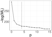
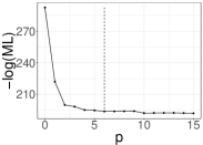
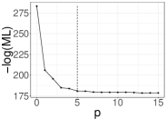
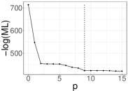
Figure 1: Negative maximum log likelihood for different AR($p$) models applied to (a)-(c): three realizations of the ARMA(1,1) model with $a=0.75,b=0.8$ of length $n=128$ and (d) the sunspot data. The respective DIC-minimizing order is visualized by a black dashed line.

Remark 4.1

Under relatively weak conditions (see e.g. Kreiss et al. (2011)) a linear process can be written as an AR($\infty$)-process with white noise errors (similarly to the famous Wold representation). Consequently, an AR($p$)-model with sufficiently large order captures the structure of a (Gaussian) linear process to any degree of accuracy. In this sense, the use of an AR-model with a sufficiently large order can be viewed as a nonparametric procedure, a fact, that has been exploited by AR-sieve-bootstrap methods for quite some time. For a recent mathematical analysis of the validity and limitations of this approach we refer to Kreiss et al. (2011).

Consequently, an AR-model can still be used for spectral density estimation under misspecification as long as the order is sufficiently large. In this sense standard order selection techniques such as DIC-minimization tend to choose large orders in this situation. However, looking at scree-like plots of the negative maximum log likelihood for increasing orders one can often see a clear bend (elbow) in the curve (with a slow decay from that point on that is not slow enough to be captured by standard penalization techniques). Similar to the use of scree plots in the context of PCA, that point can be seen as a reasonable truncation point (’elbow criterion’) where those features best explained by the parametric model have been captured. While this small model does not yet fully explain the data, adding more parameters is not helping the nonparametrically corrected procedure that we propose. In other words, we are not interested in an elaborate AR($\infty$) approximation but rather in a proxy model that captures the main parametric features of the data.

In the context of an autoregressive working model, we approximate the negative maximum log-likelihood by the negative log-likelihood evaluated at the Yule-Walker estimate. This is to ensure numerical stability and computational speed, especially for large orders. The approximation is motivated by the asymptotic equivalence of both estimates, see e.g. Chapter 8 in Brockwell and Davis (2009). The estimate is referred to as negative maximum log-likelihood in the text.

Figure 1 shows the scree-like plots for three exemplary ARMA(1,1) realizations from the above model as well as the sunspot data set. In all three realizations the elbow is clearly at $p=1$ (which is consistent with the AR-part of the model), while the DIC-criterion choses orders between 4 and 6.

Table 2 shows the simulation results for the ARMA(1,1) model and a fixed order of $p=1$. While a parametric AR($1$) model is clearly not able to explain the data (see e.g. the zero coverage of the uniform credibility intervals), this choice of the order significantly improves the results of the NPC procedure for the ARMA(1,1) data. In fact, the latter is now better than both the AR procedure as well as the NP procedure while at the same time the confidence in the model as indicated by $\hat{\eta}$ increases.

Table 2: Average Integrated Absolute Error (aIAE), Uniform 0.9-Credible Interval coverage (cUCI) and average posterior model confidence $\hat{\eta}$ for ARMA(1,1) data and fixed order $p=1$.

ARMA($1,1$): $a=0.75$, $b=0.8$ aIAE cUCI $\hat{\eta}$ $n=64$ $n=128$ $n=256$ $n=64$ $n=128$ $n=256$ $n=64$ $n=128$ $n=256$ $\operatorname{AR_{(p=1)}}$ 1.179 1.243 1.289 0 0 0 - - - $\operatorname{NPC_{(p=1)}}$ 0.942 0.741 0.586 0.986 0.969 0.954 0.601 0.635 0.670

For the sunspot data that effect can also be seen clearly as the above procedure proposes to use $p=2$ in the nonparametric procedure while the DIC-criterion suggests $p=9$. For a detailed discussion of this data analysis we refer to Section 4.2, similar effects for the LIGO data are discussed in Section 4.3.

4.2 Sunspot data

In this section, we analyse the yearly sunspot data from 1700 until 1987. We take the mean-centered version of the square root of the 288 observations as input data. We compare the AR and the NPC procedure for fixed values $p=1,2,3,9$. While $p=9$ minimises the DIC, $p=2$ captures the main AR-features of the data as indicated by the elbow criterion (see Remark 4.1 and Figure 1 (d)). The results are shown in Figure 2.

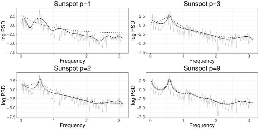
Figure 2: Posterior median spectral density estimates NPC (solid black) and AR (dashed black) for the transformed sunspot data on a logarithmic scale, for different autoregressive orders $p$. The log-periodogram is visualised in grey.

While for $p=1$ the Bernstein polynomials of the nonparametric correction cannot yet capture the peaks sufficiently well, this is clearly the case for $p=2$ (the choice obtained from the elbow criterion): While the parametric model itself can clearly not yet explain the data well, enough features are captured to improve the nonparametric correction. For larger order choices, the estimate from the NPC method does not change much anymore, so that the correction does indeed not profit from additional parameters in the AR-model. In fact for $p=9$ (as indicated by DIC), the Bayes estimator of AR and NPC are very similar.

4.3 Gravitational wave data

Gravitational waves, ripples in the fabric of spacetime caused by accelerating massive objects, were predicted by Albert Einstein in 1916 as a consequence of his general theory of relativity, see Einstein (1916). Gravitational waves originate from non-spherical acceleration of mass-energy distributions, such as binary inspiraling black holes, pulsars, and core collapse supernovae, propagating outwards from the source at the speed of light. However, they are very small (a thousand times smaller than the diameter of a proton) so that their measurement has provided decades of enormous engineering challenges.

On Sept. 14, 2015, the Laser Interferometric Gravitational Wave Observatory (LIGO), see Aasi et al. (2015), made the first direct detection of a gravitational wave signal, GW150914, originating from a binary black hole merger (Abbott et al., 2016a). The two L-shaped LIGO instruments (in Hanford, Washington and Livingston, Louisiana) each consist of two perpendicular arms, each 4 kilometers long. A passing gravitational wave will alternately stretch one arm and squeeze the other, generating an interference pattern which is measured by photo-detectors. The detector output is a time series that consists of the time-varying dimensionless strain $h(t)$, the relative change in spacing between two test masses. The strain can be modelled as a deterministic gravitational wave signal $s(t,\boldsymbol{\theta})$ depending on a vector $\boldsymbol{\theta}$ of unknown waveform parameters plus additive noise $n(t)$, such that

$$h(t)=s(t,\boldsymbol{\theta})+n(t),\quad t=1,\ldots,T.$$

There are a variety of noise sources at the LIGO detectors. This includes seismic noise, due to the motion of the mirrors from ground vibrations, earthquakes, wind, ocean waves, and vehicle traffic, thermal noise, from the microscopic fluctuations of the individual atoms in the mirrors and their suspensions, and shot noise, due to the discrete nature of light and the statistical uncertainty from the “photon counting” that is performed by the photo-detectors. In particular, LIGO noise includes high power, narrow band, spectral lines, visible as sharp peaks in the log-periodogram. As the LIGO spectrum is time-varying and subject to short-duration large-amplitude transient noise events, so-called “glitches”, a precise and realistic modelling and estimation of the noise component jointly with the signal is important for an accurate inference of the signal parameters $\boldsymbol{\theta}$. The current approach, which was also used for estimating the parameters of GW150914 in Abbott et al. (2016b), is to first use the Welch method (Welch, 1967) to estimate the spectral density from a separate stretch of data, close to but not including the signal and then to assume stationary Gaussian noise with this known spectral density in order to estimate the signal parameters.

Several approaches have been suggested in the recent gravitational wave literature to simultaneously estimate the noise spectral density and signal parameters. These include generalising the Whittle likelihood to a Student-t likelihood as in Röver et al. (2011), similarly modifying the likelihood to include additional scale parameters and then marginalising over the uncertainty in the PSD as in Littenberg et al. (2013), using cubic splines for smoothly varying broad-band noise and Lorentzians for narrow-band line features as in Littenberg and Cornish (2015), a Morlet-Gabor continuous wavelet basis for both gravitational wave burst signals and glitches as in Cornish and Littenberg (2015), the nonparametric approach of Choudhuri et al. (2004a) using a Dirichlet-Bernstein prior (Edwards et al., 2015) and a generalisation of this using a B-spline prior, see Edwards et al. (2017).

We consider 1 s of real LIGO data collected during the sixth science run (S6), recoloured to match the target noise sensitivity of Advanced LIGO (Christensen, 2010). The data is differenced and then multiplied by a Hann window to mitigate spectral leakage. A low-pass Butterworth filter (of order 20 and attenuation 0.25) is then applied before downsampling from a LIGO sampling rate of 16384 Hz to 4096 Hz, reducing the volume of data.

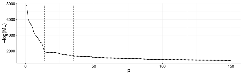
Figure 3: Negative maximum log likelihood for different AR($p$) models applied to Advanced LIGO S6 data.

We first run a pure nonparametric model, corresponding to a nonparametrically corrected likelihood with an AR(0) working model (i.e. the Whittle likelihood) to estimate the spectral density. We then compare this to a nonparametrically corrected model with an order of $p=14$, where a clear elbow can be seen in the negative log-likelihood plot (see Figure 3 and Remark 4.1). We run these simulations for 100,000 MCMC iterations, with a burn-in of 50,000, and thinning factor of 5. Results are illustrated in Figure 4 (a).

Even though $k$ converged to $k\approx 900$ mixture components, it is clear that the Bernstein-Dirichlet prior together with the Whittle likelihood is not flexible enough to estimate the sharp peaks of the LIGO spectral density. The parametric AR(14) model (estimated using the Bayesian autoregressive sampler described in Appendix B) captures the four main peaks but not their sharpness. Additionally, it does not capture the structure well in the frequency bands 0 to 450 Hz as well as larger than 1100 Hz. When compared to the AR(0) model, the nonparametrically corrected model based on $p=14$ estimates the sharp peaks much better. Furthermore, it sharpens all four peaks of the AR(14)-model (with a slight exception around 400 Hz, where seemingly two very sharp peaks overlap, a feature that is not captured by the AR(14) model at all). In the frequency bands 0 to 450 Hz as well as larger than 1100 Hz, where the parametric model fails altogether, the correction yields similar results to the nonparametric Whittle procedure. Similarly to the nonparametric Whittle procedure $k$ tends towards $k_{\max}=800$ indicating that the Bernstein-Dirichlet prior together with an AR($14$)-model is not yet flexible enough for this data set.

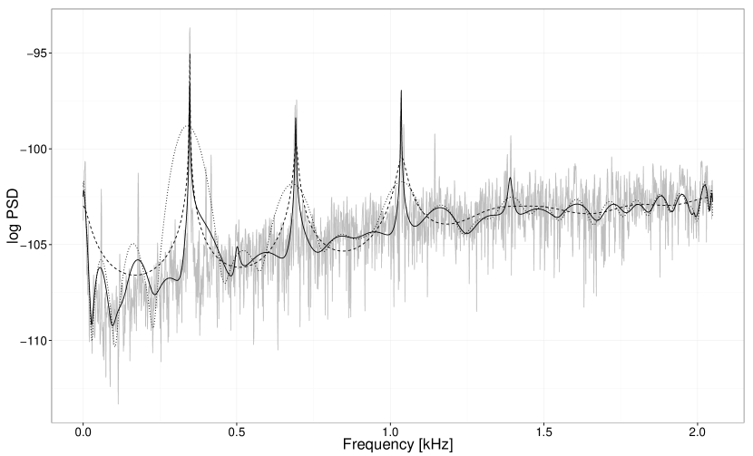
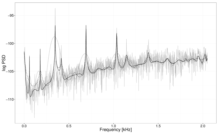
Figure 4: Estimated log spectral density for a 1 s segment of LIGO S6 data. The posterior median log spectral density estimate of NPC under an AR($p$) working model (solid black), AR($p$) (dashed black), and NPC under an AR(0) working model (dotted black) are overlaid with the log periodogram (grey), where (a) depicts $p=14$ and (b) depicts $p=35$.

Looking closer at Figure 3, the negative log-likelihood between the models AR(14) and AR(35) decreases by 533, which is not as sharp as the elbow at $p=14$, but still significant – keeping in mind that the LIGO data is a very complex data set – much more so than the ARMA(1,1) or the sunspot data. There is a moderately sized jump before $p=35$, while afterwards the descend slows down significantly. In fact the BIC chooses an order of $p=118$, where the log-likelihood reaches the level of 879, showing that the difference between $p=14$ and $p=35$ (of 533) is comparable to the one between $p=35$ and $p=128$ (of 512). This indicates that there is indeed another change of gradient around $p=35$. When looking at penalized likelihoods, this is also the point, where different penalizations start to obviously diverge. The results for $p=35$ can be found in Figure 4 (b).

The parametric AR($35$) model already provides a reasonable fit to the periodogram, picking up the major peaks (with the exception around 100 Hz), but under- and overestimates some of the peaks. In particular there are still major problems in the frequency bands 0 to 300 Hz and 400 to 700 Hz. The NPC procedure with $p=35$ keeps the peaks that have been capture well by the parametric model but corrects problems most prominently in the above mentioned frequency bands. It is worth mentioning that the correction works in several ways: Sharpening existing peaks (e.g. at 0 Hz), adding new peaks (e.g. at 100 Hz) as well as smoothing out some erroneous peaks (e.g. at 600 Hz). Overall, the resulting estimate seems to capture the structure quite well in all frequency bands. This impression is complemented by the results of the NPC method with AR($35$) working model together with the pointwise and uniform credible bounds obtained from the procedure in Figure 5.

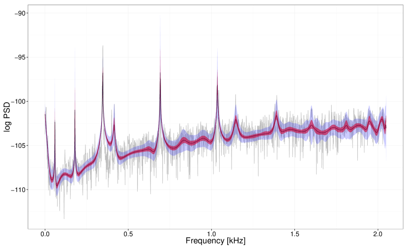
Figure 5: Estimated log spectral density for a 1 s segment of LIGO S6 data. The posterior median log spectral density estimate of NPC under an AR(35) working model (solid black), pointwise 0.9-credible region (shaded red), and uniform 0.9-credible region (shaded violet) are overlaid with the log periodogram (grey).

5 Conclusion

In this work we propose a nonparametric correction of a parametric likelihood to obtain an approximation of the true (inaccessible) likelihood of a stationary time series. This approach extends the famous approximation by Whittle. For Gaussian data, the Whittle likelihood, the nonparametric correction as well as the true likelihood are asymptotically equivalent. Secondly, we propose a Bayesian procedure for spectral density estimation, where a parametric likelihood is used with a Bayesian nonparametric spectral correction. We show consistency of the resulting pseudo-posterior distribution for a fixed parametric likelihood. Furthermore, we present a Bayesian semiparametric procedure that combines inference about the parametric working model with the nonparametric correction. The extent of the contribution of the parametric spectral density to the spectral density estimate is controlled by a shape confidence parameter. Simulation results have shown that this procedure inherits the benefits from the parametric working model if the latter is well-specified or describe a part of the features of the data well, while in the misspecified case the results are comparable to the usage of the Whittle likelihood.

Regarding future work, it is interesting to investigate whether in the non-Gaussian case the class of time series for which asymptotically consistent inference holds can be enlarged by choosing an appropriate model. It is important to understand the distributional influence in the non-Gaussian case both in finite samples and asymptotically. As an example, in a bootstrap context, it suffices to capture the fourth order structure of a linear model to obtain asymptotically valid second-order frequentist properties of the autocovariance structure Dahlhaus and Janas (1996); Kreiss and Paparoditis (2003). As suggested by Kleijn et al. (2012) in a parametric setting, this property does not simply carry over to a Bayesian context. Preliminary results for non-Gaussian autoregressive time series however have shown considerable benefits (with respect to first and second order frequentist properties) when the innovation distribution is well-specified in comparison to a Gaussian model. Since any parametric likelihood is susceptible to misspecification, the ultimate goal is to consider a Bayesian nonparametric model for the innovation distribution, such as Dirichlet mixtures of normals. Further directions for future work are automation of the elbow criterion discussed in Remark 4.1. Instead of choosing a fixed order in advance, an automation might as well serve as a guideline for specifying a prior on the AR order parameter, which can be included in the inference by means of RJMCMC (c.f. Remark 3.3).

Appendix A Appendix: Proofs

Proof A.1 (of (4)).

Since $F_{n}$ is orthonormal it holds $|\det F_{n}|=1$ and hence by an application of the transformation theorem

$$p^{W}_{\mathbf{Z}_{n}=F_{n}^{T}\mathbf{\tilde{Z}}_{n}}(\mathbf{z}_{n}|f) = |\det F_{n}|\;p_{\mathbf{\tilde{Z}}_{n}}^{W}(F_{n}\mathbf{z}_{n}|f)\propto\det(D_{n})^{-1/2}\exp\left(-\frac{1}{2}\boldsymbol{\tilde{z}}_{n}^{T}D_{n}^{-1}\boldsymbol{\tilde{z}}_{n}\right)$$

$$\propto \exp\left(-\frac{1}{2}\sum_{j=0}^{n-1}\log f(\lambda_{j})-\frac{1}{2}\boldsymbol{\tilde{z}}_{n}^{T}D_{n}^{-1}\boldsymbol{\tilde{z}}_{n}\right),$$

where $\boldsymbol{\tilde{z}}_{n}=F_{n}\boldsymbol{z}_{n}$. Finally, by (2.1), $I_{n}(\lambda_{k})=I_{n}(\lambda_{n-k})$ as well as $f(\lambda_{k})=f(\lambda_{n-k})$ it holds

$$\boldsymbol{\tilde{z}}_{n}^{T}D_{n}^{-1}\boldsymbol{\tilde{z}}_{n}=\frac{\tilde{z}_{n}^{2}(0)}{2\pi f(0)}+\frac{\tilde{z}_{n}^{2}(n/2)}{2\pi f(\pi)}1_{\{n\text{ even}\}}+\sum_{j=1}^{N}\frac{\tilde{z}^{2}_{n}(2j-1)+\tilde{z}^{2}_{n}(2j)}{2\pi f(\lambda_{j})}$$

$$=\frac{I_{n,\lambda_{0}}(\boldsymbol{z})}{f(0)}+\frac{I_{n,\lambda_{n/2}}(\boldsymbol{z})}{f(\pi)}1_{\{n\text{ even}\}}+\sum_{j=1}^{N}\frac{2I_{n,\lambda_{j}}(\boldsymbol{z})}{f(\lambda_{j})}=\sum_{j=0}^{n-1}\frac{I_{n,\lambda_{j}}(\boldsymbol{z})}{f(\lambda_{j})},$$

yielding the assertion.

Proof A.2 (of Remark 2.1).

The spectral density corresponding to a Gaussian white noise with variance $\sigma^{2}$ is given by $\sigma^{2}/2\pi$, hence $\sigma^{2}\,C_{n}=D_{n}$ and

$$p_{\text{i.i.d. }N(0,\sigma^{2})}^{C}(\mathbf{Z}_{n}|f) \propto\frac{\det C_{n}^{-1/2}}{\sigma^{n}}\exp\left(-\frac{1}{2\sigma^{2}}\mathbf{Z}_{n}^{T}F_{n}^{T}C_{n}^{-1/2}F_{n}F_{n}^{T}C_{n}^{-1/2}F_{n}\mathbf{Z}_{n}\right)$$

$$\propto\det D_{n}^{-1/2}\exp\left(-\frac{1}{2}(F_{n}\mathbf{Z}_{n})^{T}D_{n}^{-1}(F_{n}\mathbf{Z}_{n})\right),$$

which can be shown to be the Whittle likelihood analogously to the proof of equation 4 since $F_{n}\mathbf{Z}_{n}=\boldsymbol{\tilde{Z}}_{n}$.

Proof A.3 (of Proposition 2.1).

If $f=f_{\text{param}}$ then $C_{n}=\text{Id}$ and $F_{n}^{T}C_{n}^{-1/2}F_{n}=\text{Id}$, hence a) follows. For b), consider a time series distributed according to the corrected likelihood, i.e. $\mathbf{X}_{n}=(X_{1},\ldots,X_{n})\sim p_{\text{param}}^{C}$. An application of the transformation theorem shows that $\mathbf{Y}_{n}=F_{n}^{T}C_{n}^{-1/2}F_{n}\mathbf{X}_{n}\sim p_{\text{param}}$ on noting that $(F_{n}^{T}C_{n}^{-1/2}F_{n})^{-1}=F_{n}^{T}C_{n}^{1/2}F_{n}$ and $\operatorname{det}((F_{n}^{T}C_{n}^{-1/2}F_{n})^{-1})=\sqrt{\mbox{det}(C_{n})}$. By (2.1) it holds

$$I_{n,\lambda_{j}}(\mathbf{X}_{n})=I_{n,\lambda_{j}}(F_{n}^{T}C_{n}^{1/2}F_{n}\mathbf{Y}_{n})=\frac{f(\lambda_{j})}{f_{\text{param}}(\lambda_{j})}\,I_{n,\lambda_{j}}(\mathbf{Y}_{n})$$

as $F_{n}(F_{n}^{T}C_{n}^{1/2}F_{n}\mathbf{Y}_{n})=C_{n}^{1/2}(F_{n}\mathbf{Y}_{n})$. By Brockwell and Davis [2009], Proposition 10.3.1., it holds $\operatorname{E}I_{n,\lambda_{j}}(\mathbf{Y}_{n})=f_{\text{param}}(\lambda_{j})+o(1)$ where convergence is uniform in $j$ (recall that the time series is mean zero). From this the assertion follows because $f_{\text{param}}$ is bounded from below by assumption.

Proof A.4 (of Theorem 3.1).

Choudhuri et al. [2004b] proved mutual contiguity of the true Gaussian and the Whittle likelihood in the frequency domain which carries over to the time domain by an application of the transformation theorem because $F_{n}$ is bijective. Hence, it is sufficient to show mutual contiguity of the corrected parametric likelihood and the Whittle likelihood. Following the proof of Theorem 1 in Choudhuri et al. [2004b] it is enough to show that their log-likelihood ratio is a tight sequence under both $p^{C}$ as well as $p^{W}$. To this end, note that it holds

$$p^{W}\propto\det D_{n}^{-1/2}\exp\left(-\frac{1}{2}\mathbf{Z}_{n}^{T}F_{n}^{T}D_{n}^{-1}F_{n}\mathbf{Z}_{n}\right),$$

$$p^{C}\propto\det C_{n}^{-1/2}\;\det\Sigma_{n,\text{param}}^{-1/2}\exp\left(-\frac{1}{2}\mathbf{Z}_{n}^{T}F_{n}^{T}C_{n}^{-1/2}F_{n}\Sigma_{n,\text{param}}^{-1}F_{n}^{T}C_{n}^{-1/2}F_{n}\mathbf{Z}_{n}\right),$$

where $\Sigma_{n,\text{param}}$ is the covariance matrix of the corresponding parametric time series, e.g. for the AR($p$)-case the covariance matrix associated with likelihood (6). Hence, the log-likelihood ratio is given by

$$\frac{1}{2}\left(\log\det D_{n}-\log\det C_{n}-\log\det\Sigma_{n,\text{param}}\right)$$

$$+\frac{1}{2}\left(\mathbf{Z}_{n}^{T}F_{n}^{T}D_{n}^{-1}F_{n}\mathbf{Z}_{n}-\mathbf{Z}_{n}^{T}F_{n}^{T}C_{n}^{-1/2}F_{n}\Sigma_{n,\text{param}}^{-1}F_{n}^{T}C_{n}^{-1/2}F_{n}\mathbf{Z}_{n}\right)=:\frac{1}{2}A_{n}+\frac{1}{2}B_{n}(\mathbf{Z}_{n}).$$

Defining $D_{n,\text{param}}$ analogously to $D_{n}$ as in (3) with the nonparametric spectral density $f$ replaced by the parametric version $f_{\text{param}}$ as e.g. for AR($p$) given in (7), we get

$$A_{n}=\log\det D_{n,\text{param}}-\log\det\Sigma_{n,\text{param}}=O(1),$$

where the boundedness follows from Lemma A.1 in Choudhuri et al. [2004b]. To obtain stochastic boundedness of $B_{n}(\mathbf{Z}_{n})$ under $p^{W}$ as well as $p^{C}$ we will show boundedness of the expectation and variance. Following Choudhuri et al. [2004b] we get under $p^{W}$ (i.e. $F_{n}\mathbf{Z}_{n}\sim N(0,D_{n})$)

$$\operatorname{E}B_{n}(\mathbf{Z}_{n})=\mbox{tr}\left(I_{n}-C_{n}^{-1/2}F_{n}\Sigma^{-1}_{n,\text{param}}F_{n}^{T}C_{n}^{-1/2}D_{n}\right).$$

Because $\mbox{tr}(AB)=\mbox{tr}(BA)$, it holds by $C_{n}^{-1/2}D_{n}C_{n}^{-1/2}=D_{n,\text{param}}$

$$\mbox{tr}(C_{n}^{-1/2}F_{n}\Sigma^{-1}_{n,\text{param}}F_{n}^{T}C_{n}^{-1/2}D_{n})=\mbox{tr}(F_{n}\Sigma^{-1}_{n,\text{param}}F_{n}^{T}D_{n,\text{param}}),$$ (12)

the assertion follows by Lemma A.2 in Choudhuri et al. [2004b] by the linearity of the trace. Similar arguments yield the assertion under $p^{C}$ (i.e. $\mathbf{Z}_{n}\sim N(0,F_{n}^{T}C_{n}^{1/2}F_{n}\Sigma_{n,\text{param}}F_{n}^{T}C_{n}^{1/2}F_{n}))$ noting that

$$\operatorname{E}B_{n}(\mathbf{Z}_{n})=\mbox{tr}\left(F_{n}^{T}D_{n}^{-1}C_{n}^{1/2}F_{n}\Sigma_{n,\text{param}}F_{n}^{T}C_{n}^{1/2}F_{n}-I_{n}\right)=\mbox{tr}\left(D_{n,\text{param}}^{-1}F_{n}\Sigma_{n,\text{param}}F_{n}^{T}-I_{n}\right).$$

Concerning the variance we get under $p^{W}$

$$\operatorname{Var}B_{n}(\mathbf{Z}_{n})=2\,\mbox{tr}\left(\left(I_{n}-C_{n}^{-1/2}F_{n}\Sigma^{-1}_{n,\text{param}}F_{n}^{T}C_{n}^{-1/2}D_{n}\right)^{2}\right).$$

Similar arguments as above yield

$$\mbox{tr}\left(\left(C_{n}^{-1/2}F_{n}\Sigma^{-1}_{n,\text{param}}F_{n}^{T}C_{n}^{-1/2}D_{n}\right)^{2}\right)=\mbox{tr}\left(\left(F_{n}\Sigma_{n,\text{param}}^{-1}F_{n}^{T}D_{n,\text{param}}\right)^{2}\right).$$

Together with (12) this yields

$$\operatorname{Var}B_{n}(\mathbf{Z}_{n})=2\,\mbox{tr}\left(\left(I_{n}-F_{n}\Sigma_{n,\text{param}}^{-1}F_{n}^{T}D_{n,\text{param}}\right)^{2}\right)$$

by $\mbox{tr}((I_{n}-A)^{2})=\mbox{tr}(I)-2\mbox{tr}(A)+\mbox{tr}(A^{2})$. Hence, the assertion follows by Lemma A.2 in Choudhuri et al. [2004b]. Analogous assertions yield the result under $p^{C}$.

Ghosal et al. [1999] give sufficient conditions for the consistency of the posterior distribution when using Bernstein polynomial priors in terms of the existence of exponentially powerful tests for testing $H_{0}:\theta=\theta_{0}$ and prior positivity of a Kullback-Leibler neighbourhood. But these require i.i.d. observations. To prove posterior consistency under the Whittle likelihood, Choudhuri et al. [2004a] extend this result to independent but not identically distributed observations and apply this to the periodogram ordinates which are independent exponential random variables under the Whittle likelihood. However, periodogram ordinates under the corrected likelihood are no longer independent, therefore this theorem is not applicable. We give an extension to non-independent random variables in the following theorem, which is needed to prove Theorem 3.2:

Theorem A.5.

Let $\mathbf{Z}_{n}=(Z_{1,n},\ldots,Z_{n,n})$ be random vectors with probability distribution $P^{n}_{\theta}$ and corresponding pdf $p_{n}(\cdot|\theta)$. Let $\theta_{0}\in\Theta$, $U_{n}\in{\cal T}$, where ${\cal T}$ denotes the Borel $\sigma$-algebra on $\Theta$, and $\Pi$ a probability distribution on $(\Theta,{\cal T})$. Define

$$K_{n}(\theta_{0},\theta) = \operatorname{E}_{\theta_{0}}\left[\log\frac{p_{n}(\mathbf{Z}_{n}|\theta_{0})}{p_{n}(\mathbf{Z}_{n}|\theta)}\right]\mbox{ and }$$

$$V_{n}(\theta_{0},\theta) = \operatorname{Var}_{\theta_{0}}\left[\log\frac{p_{n}(\mathbf{Z}_{n}|\theta_{0})}{p_{n}(\mathbf{Z}_{n}|\theta)}\right].$$

Under the following assumptions of prior positivity of neighbourhoods and existence of tests:

• There exists a set $B\in{\cal T}$ with $\Pi(B)>0$ such that

  • $\frac{1}{n^{2}}V_{n}(\theta_{0},\theta)\rightarrow 0\qquad\mbox{for all }\theta\in B$, and

  • $\lim\inf_{n\rightarrow\infty}\Pi(\{\theta\in B:\frac{1}{n}K_{n}(\theta_{0},\theta)<\epsilon\})>0\qquad\forall\epsilon>0$.

• There exists test functions $\{\phi_{n}\}$, subsets $\Theta_{n}\subset\Theta$, and constants $K_{1},K_{2},k_{1},k_{2}>0$ such that

  • $\operatorname{E}_{\theta_{0}}\phi_{n}\rightarrow 0$.

  • $\sup_{\theta\in U_{n}^{c}\cap\Theta_{n}}\operatorname{E}_{\theta}(1-\phi_{n})\leq K_{1}\exp^{-k_{1}n}$, and

  • $\Pi(\Theta_{n}^{c})\leq K_{2}\exp^{-k_{2}n}.$

Then

$$\Pi(\theta\in U_{n}^{c}|\mathbf{Z}_{n})\rightarrow 0\qquad\mbox{in }P_{\theta_{0}}^{n}\mbox{-probability}.$$

Proof A.6.

The proof is completely analogous to the proof of Theorem A.1 in Choudhuri et al. [2004a].

The following lemma replaces Lemma B.3 in Choudhuri et al. [2004a].

Lemma A.7.

Let $\mathbf{Z}_{n}\sim N(0,F_{n}^{T}D_{n}(f)^{1/2}S_{n}D_{n}(f)^{1/2}F_{n})$ where $S_{n}$ is a symmetric positive definite matrix and $D_{n}(f)=\mbox{diag}(f(\lambda_{1}),\ldots,f(\lambda_{n}))$. With $c(\lambda_{i})=f(\lambda_{i})/f_{\text{param}}(\lambda_{i})^{\eta}$ consider testing

$$H_{0}:c(\lambda_{i})=c_{0}(\lambda_{i}),\quad\mbox{ where }c_{0}(\lambda_{i})\leq a\quad\mbox{ for }i=1,\ldots,n,\quad\mbox{ against }$$

$$H_{1}:c(\lambda_{i})=c_{1}(\lambda_{i}),\quad\mbox{ where }c_{1}(\lambda_{i})<c_{0}(\lambda_{i})-\epsilon\quad\mbox{ for }i=1,\ldots,n,$$

where $a>\epsilon>0$ do not depend on $n$. Then there exists a test $\phi_{n}$ and constants $\beta_{1},\beta_{2}>0$ depending only on $a$ and $\epsilon$ such that

$$\operatorname{E}_{H_{0}}(\phi_{n})\leq\exp^{-\beta_{1}n}\qquad\mbox{ and}\qquad\operatorname{E}_{H_{1}}(1-\phi_{n})\leq\exp^{-\beta_{2}n}.$$

Proof A.8.

Consider a test $\phi_{n}$ that rejects $H_{0}$ if

$$T_{n}=\mathbf{Z}_{n}^{T}F_{n}^{T}D_{n}(f_{0})^{-1/2}S_{n}^{-1}D_{n}(f_{0})^{-1/2}F_{n}\mathbf{Z}_{n}<nx$$

with a critical value $x>0$ with $x\neq 1$ and $x\neq 1-\epsilon/a$.

Denote $\mathbf{Y}_{n}\sim N(0,I_{n})$, then

$$T_{n}\overset{\mathcal{D}}{\underset{H_{0}}{=}}\mathbf{Y}_{n}^{T}\mathbf{Y}_{n}\overset{\mathcal{D}}{\underset{H_{0}}{=}}\chi^{2}_{n}.$$

Consequently, the moment generating function of $T_{n}$ under $H_{0}$ is given by $E\left[\exp^{tT_{n}}\right]=(1-2t)^{-n/2}$ and exists for $t<1/2$. By an application of the Markov inequality, we get for all $z>0$

$$P_{c_{0}}\left(T_{n}<nx\right)=P_{c_{0}}\left(e^{-zT_{n}}>e^{-nzx}\right)\leq\exp^{nzx}\operatorname{E}_{c_{0}}\left[\exp^{-zT_{n}}\right]=e^{-n[-zx+\frac{1}{2}\log(1+2z)]}.$$

The function $g_{1}(z)=-zx+\frac{1}{2}\log(1+2z)$ attains its maximum at $z_{1}=\frac{1-x}{2x}>0$ and

$$g_{1}(z_{1})=-\frac{1-x}{2}+\frac{1}{2}\log\left(1+\frac{1-x}{x}\right)>-\frac{1-x}{2}+\frac{1-x}{2}=0$$

as $\log(1+y)>\frac{y}{1+y}$ for $y\neq 0$. Thus, setting $\beta_{1}=g_{1}(z_{1})>0$, we obtain

$$\operatorname{E}_{H_{0}}(\phi_{n})=P_{c_{0}}\left(T_{n}<nx\right)\leq e^{-n\beta_{1}}.$$

Similarly, under $H_{1}$, we get

$$T_{n}\overset{\mathcal{D}}{\underset{H_{1}}{=}}\mathbf{Y}_{n}^{T}BB^{T}\mathbf{Y}_{n},\qquad\text{with }B=S_{n}^{1/2}D_{n}(f_{1}/f_{0})^{1/2}S_{n}^{-1/2}.$$

Since

$$\mbox{det}(B-\lambda I_{n})=\mbox{det}(S_{n}^{1/2}[D_{n}^{1/2}(f_{1}/f_{0})-\lambda I_{n}]S_{n}^{-1/2})=\mbox{det}(D_{n}^{1/2}(f_{1}/f_{0})-\lambda I_{n})$$

the matrix $B$ has the eigenvalues $(c_{1}(\lambda_{i})/c_{0}(\lambda_{i}))^{1/2}=(f_{1}(\lambda_{i})/f_{0}(\lambda_{i}))^{1/2}$, $i=1,\ldots,n$. Since $B$ is a normal matrix (recall that $S_{n}$ is symmetric positive definite), we find that $BB^{T}$ has the eigenvalues $c_{1}(\lambda_{i})/c_{0}(\lambda_{i})$, $i=1,\ldots,n$. Consequently,

$$T_{n}\overset{\mathcal{D}}{\underset{H_{1}}{=}}\mathbf{Y}_{n}^{T}BB^{T}\mathbf{Y}_{n}\overset{\mathcal{D}}{\underset{H_{1}}{=}}\mathbf{Y}_{n}^{T}D_{n}(f_{1}/f_{0})\mathbf{Y}_{n}\leq\mathbf{Y}_{n}^{T}\mathbf{Y}_{n}\,\max_{1\leq i\leq n}\frac{c_{1}(\lambda_{i})}{c_{0}(\lambda_{i})}<\mathbf{Y}_{n}^{T}\mathbf{Y}_{n}\,\max_{1\leq i\leq n}\frac{c_{0}(\lambda_{i})-\epsilon}{c_{0}(\lambda_{i})}$$

$$\leq\left(1-\frac{\epsilon}{a}\right)\,\mathbf{Y}_{n}^{T}\mathbf{Y}_{n}.$$

Consequently,

$$\operatorname{E}_{H_{1}}(1-\phi_{n})=P_{c_{1}}\left(T_{n}\geq nx\right)\leq P_{c_{1}}\left(\mathbf{Y}_{n}^{T}\mathbf{Y}_{n}\geq\frac{nx}{1-\epsilon/a}\right).$$

Analogously to the proof under the null hypothesis, we get for any $z<1/2$

$$P_{c_{1}}\left(\mathbf{Y}_{n}^{T}\mathbf{Y}_{n}\geq\frac{nx}{1-\epsilon/a}\right)\leq e^{-n\left(\frac{zx}{1-\epsilon/a}+\frac{1}{2}\log(1-2z)\right)}.$$

Now $g_{2}(z)=zy+\frac{1}{2}\log(1-2z)$, $y=x/(1-\epsilon/a)$, attains its maximum at $z_{2}=\frac{y-1}{2y}<\frac{1}{2}$ with

$$g_{2}(z_{2})=\frac{y-1}{2}-\frac{1}{2}\log y>0$$

as $\log y<y-1$ for $y\neq 1$, i.e. $x\neq 1-\epsilon/a$. Setting $\beta_{2}=g_{2}(z_{2})>0$ yields $\operatorname{E}_{H_{1}}(1-\phi_{n})\leq e^{-\beta_{2}n}$, completing the proof.

Proof A.9 (of Theorem 3.2).

We follow Choudhuri et al. [2004a], proof of Theorem 1, and show (C1) and (C2) of Theorem A.5 above. Let $p_{n}(\mathbf{Z}_{n}|c)$ denote the corrected likelihood and define $a=||c_{0,\eta}||_{\infty}=\sup_{\lambda\in[0,\pi]}|c_{0,\eta}(\lambda)|$ and $b=\inf_{\lambda\in[0,\pi]}|c_{0,\eta}(\lambda)|$. An analogous argument as in Appendix B.1. of Choudhuri et al. [2004a] shows that for all $\epsilon>0$ the set $\{c:||c-c_{0,\eta}||_{\infty}<\epsilon\}$ has positive prior probability under the Bernstein polynomial prior on $\Theta$. We need to show (C1)(a) and (b). To this end, let $c\in B$ where

$$B=\{c:||c-c_{0,\eta}||_{\infty}<b/2\}.$$

For $c\in B$ we have $c>b/2$. To prove (C1), first note that

$$\log\frac{p_{n}(\mathbf{Z}_{n}|c_{0,\eta})}{p_{n}(\mathbf{Z}_{n}|c)} =\frac{1}{2}\sum_{i=1}^{n}\log\frac{f(\lambda_{i})}{f_{0}(\lambda_{i})}-\frac{1}{2}\mathbf{Z}_{n}^{T}F_{n}^{T}D_{n}^{-1/2}(f_{0})S_{n}^{-1}D_{n}^{-1/2}(f_{0})F_{n}\mathbf{Z}_{n}$$

$$\quad+\frac{1}{2}\mathbf{Z}_{n}^{T}F_{n}^{T}D_{n}^{-1/2}(f)S_{n}^{-1}D_{n}^{-1/2}(f)F_{n}\mathbf{Z}_{n}$$

where $S_{n}=D_{n}^{-1/2}(f_{\text{param}})F_{n}\Sigma_{n,\text{param}}F_{n}^{T}D_{n}(f_{\text{param}})^{-1/2}$. For $\mathbf{Y}_{n}\overset{\mathcal{D}}{=}N(0,\Sigma)$ it holds $\operatorname{E}\mathbf{Y}_{n}^{T}A\mathbf{Y}_{n}=\mbox{tr}(A\Sigma)$ as well as $\operatorname{Var}(\mathbf{Y}_{n}^{T}A\mathbf{Y}_{n})=2\mbox{tr}(A\Sigma A\Sigma)$. Furthermore, by analogous argument as in the proof of Lemma A.7 we get that the eigenvalues of

$$F_{n}^{T}D_{n}(f)^{-1/2}S_{n}^{-1}D_{n}(f_{0}/f)^{1/2}S_{n}D_{n}(f_{0})^{1/2}F_{n}$$

are given by $f_{0}(\lambda_{i})/f(\lambda_{i})=c_{0,\eta}(\lambda_{i})/c(\lambda_{i})$, $i=1,\ldots,n$, hence

$$\mbox{tr}(F_{n}^{T}D_{n}(f)^{-1/2}S_{n}^{-1}D_{n}(f_{0}/f)^{1/2}S_{n}D_{n}(f_{0})^{1/2}F_{n})=\sum_{i=1}^{n}\frac{c_{0,\eta}(\lambda_{i})}{c(\lambda_{i})}.$$

As a consequence, we get

$$0 \leq\frac{1}{n}K_{n}(c_{0},c)=\frac{1}{2n}\sum_{i=1}^{n}\log\frac{f(\lambda_{i})}{f_{0}(\lambda_{i})}-\frac{1}{2}+\frac{1}{2n}\mbox{tr}(F_{n}^{T}D_{n}(f)^{-1/2}S_{n}^{-1}D_{n}(f_{0}/f)^{1/2}S_{n}D_{n}(f_{0})^{1/2}F_{n})$$

$$=\frac{1}{2n}\sum_{i=1}^{n}\log\left(\frac{c(\lambda_{i})-c_{0,\eta}(\lambda_{i})}{c_{0,\eta}(\lambda_{i})}+1\right)+\frac{1}{2n}\sum_{i=1}^{n}\left(\frac{c_{0,\eta}(\lambda_{i})-c(\lambda_{i})}{c(\lambda_{i})}+1\right)-\frac{1}{2}$$

$$=O(1)\;\|c-c_{0,\eta}\|_{\infty}.$$

Similar arguments yield

$$0\leq\frac{1}{n^{2}}V_{n}(c_{0,\eta},c)=\frac{1}{2n^{2}}\mbox{tr}\left[\left(I_{n}-F_{n}^{T}D_{n}(f)^{-1/2}S_{n}^{-1}D_{n}^{1/2}(f_{0}/f)S_{n}D_{n}(f_{0})^{1/2}F_{n})\right)^{2}\right]$$

$$=\frac{1}{2n^{2}}\sum_{i=1}^{n}\left(\frac{c_{0,\eta}(\lambda_{i})-c(\lambda_{i})}{c(\lambda_{i})}\right)^{2}=O(1/n)\;\|c-c_{0,\eta}\|_{\infty}^{2}\to 0.$$

The proof can now be concluded as in Choudhuri et al. [2004a] by replacing Lemma B.3 by Lemma A.7 above.

Appendix B Appendix: Bayesian autoregressive sampler

For fixed order $p\geq 0$, the autoregressive model $Z_{t}=\sum_{l=1}^{p}a_{l}Z_{t-l}+e_{t}$ with i.i.d. N($0,\sigma^{2}$) random variables is parametrized by the the innovation variance $\sigma^{2}$ and the partial autocorrelation structure $\mathbf{\boldsymbol{\rho}}=(\rho_{1},\ldots,\rho_{p})$, where $\rho_{k}$ is the conditional correlation between $Z_{t}$ and $Z_{t+k}$ given $Z_{t+1},\ldots,Z_{t+k-1}$. Note that $\mathbf{\boldsymbol{\rho}}\in(-1,1)^{p}$ and that there is a one-to-one relation between $\mathbf{a}=(a_{1},\ldots,a_{p})$ and $\boldsymbol{\rho}$. To elaborate, we follow Barndorff-Nielsen and Schou [1973] and introduce the auxiliary variables $\phi_{k,l}$ as solutions of the following Yule-Walker-type equation with the autocorrelations $r_{k}=\operatorname{E}[Z_{t}Z_{t+k}]/\operatorname{E}Z_{1}^{2}$:

$$\begin{pmatrix}1&r_{1}&\ldots&r_{k-1}\\ r_{1}&1&\ldots&r_{k-2}\\ \vdots&\vdots&\ddots&\vdots\\ r_{k-1}&r_{k-2}&\ldots&1\end{pmatrix}\begin{pmatrix}\phi_{k,1}\\ \phi_{k,2}\\ \vdots\\ \phi_{k,k}\end{pmatrix}=\begin{pmatrix}r_{1}\\ r_{2}\\ \vdots\\ r_{k}\end{pmatrix}.$$

As shown in Barndorff-Nielsen and Schou [1973], the well-known relationships

$$\phi_{p,l} =a_{l},\quad l=1,\ldots,p,$$

$$\phi_{k,k} =\rho_{k},\quad k=1,\ldots,p$$

readily imply $a_{p}=\rho_{p}$ and (recall that $\rho_{k}=0$ for $k>p$) the recursive formula

$$a_{l}=\rho_{l}-\rho_{l+1}\phi_{l,1}-\rho_{l+2}\phi_{l+1,2}-\ldots-\rho_{p}\phi_{p-1,p-l},\quad l=1,\ldots,p-1.$$

We specify the following prior assumptions for the model parameters:

$$\rho_{l} \sim\text{uniform}((-1,1)),\quad 1\leq l\leq p,$$

$$\sigma^{2} \sim\text{inverse-gamma}(\alpha_{\sigma},\beta_{\sigma}),$$

all a priori independent. We use $\alpha_{\sigma}=\beta_{\sigma}=0.001$. Furthermore, we employ the Gaussian likelihood

$$p(\mathbf{Z}_{n}|\mathbf{\rho},\sigma^{2}) =\det\Sigma_{p,\mathbf{a},\sigma^{2}}^{-1/2}\exp\left\{-\frac{1}{2}\mathbf{Z}_{p}^{T}\Sigma_{p,\mathbf{a},\sigma^{2}}^{-1}\mathbf{Z}_{p}\right\}\prod_{i=p+1}^{n}\phi_{\sigma}\left(Z_{i}-\sum_{l=1}^{p}a_{l}Z_{i-l}\right)$$

with the N($0,\sigma^{2}$) density $\phi_{\sigma}(\cdot)$ and the $p\times p$ autocovariance matrix $\Sigma_{p,\mathbf{a}(\mathbf{\rho})}$ of the autoregressive model. To draw samples from the corresponding posterior distribution, we use a Gibbs sampler, where the conjugate full conditional for $\sigma^{2}$ is readily sampled. For $j=1,\ldots,p$ the full conditional for $\rho_{j}$ is sampled with the Metropolis algorithm using a normal random walk proposal density with proposal variance $\sigma_{l}^{2}$. As for the parameters of the working model within the corrected parametric approach (see Section 3.4), the proposal variances are adjusted adaptively during the burn-in period, aiming for a respective acceptance rate of 0.44.

Appendix C Appendix: Further simulation results

Table 2 depicts further results of the AR, NP and NPC procedures for normal ARMA data.

Table 3: Average Integrated Absolute Error (aIAE), Uniform Credible Interval coverage (cUCI) and average posterior model confidence $\hat{\eta}$ for different realizations of model (11).

White Noise: $a=b=0$ MA($2$): $b_{1}=0.75$, $b_{2}=-0.5$ AR($2$): $a_{1}=0.75$, $a_{2}=-0.5$ Methods $n=64$ $n=128$ $n=256$ $n=64$ $n=128$ $n=256$ $n=64$ $n=128$ $n=256$ aIAE AR 0.095 0.074 0.053 0.343 0.278 0.221 0.270 0.201 0.150 NP 0.102 0.066 0.042 0.233 0.177 0.128 0.314 0.257 0.207 NPC 0.104 0.070 0.047 0.236 0.180 0.137 0.276 0.211 0.163 cUCI AR 1.000 0.999 0.999 0.771 0.757 0.786 0.996 1.000 1.000 NP 1.000 1.000 1.000 0.999 0.999 0.992 0.998 0.992 0.982 NPC 1.000 1.000 1.000 1.000 1.000 1.000 0.999 1.000 1.000 $\hat{\eta}$ 0.368 0.325 0.293 0.293 0.199 0.123 0.461 0.529 0.614

For white noise, all procedures yield good results, whereas NP is superior due to the implicitly well-specified white noise working model (recall that the order $p$ within AR and NPC are estimated with the DIC). The results for MA(2) data are qualitatively similar to the results for MA(1) data in Table 1. The spectral peaks of the AR(2) model are not as strong as the spectral peak of the AR(1) model considered in Table 1. Accordingly, it can be seen that the NP results are better in this case. The NPC benefits again from the well-specified parametric model, yielding results that are comparable to the AR procedure.

References

- Aasi et al. [2015] J. Aasi et al. Advanced LIGO. Classical and Quantum Gravity, 32:074001, 2015.
- Abbott et al. [2016a] B. P. Abbott et al. Observation of gravitational waves from a binary black hole merger. Physical Review Letters, 116:061102, 2016a.
- Abbott et al. [2016b] B. P. Abbott et al. Properties of the binary black hole merger GW150914. Physical Review Letters, 116:241102, 2016b.
- Barndorff-Nielsen and Schou [1973] O. Barndorff-Nielsen and G. Schou. On the parametrization of autoregressive models by partial autocorrelations. Journal of Multivariate Analysis, 3(4):408–419, 1973.
- Barnett et al. [1996] G. Barnett, R. Kohn, and S. Sheather. Bayesian estimation of an autoregressive model using Markov chain Monte Carlo. Journal of Econometrics, 74(2):237–254, 1996.
- Bauwens et al. [2000] L. Bauwens, M. Lubrano, and J.-F. Richard. Bayesian inference in dynamic econometric models. Oxford University Press, 2000.
- Bollerslev [1986] T. Bollerslev. Generalized autoregressive conditional heteroskedasticity. Journal of Econometrics, 31(3):307–327, 1986.
- Box et al. [2013] G. E. P. Box, G. M. Jenkins, and G. C. Reinsel. Time series analysis: Forecasting and control. John Wiley & Sons, 2013.
- Brockwell and Davis [2009] P. J. Brockwell and R. A. Davis. Time series: Theory and methods. Springer, 2009.
- Carter and Kohn [1997] C.K. Carter and R. Kohn. Semiparametric Bayesian inference for time series with mixed spectra. Journal of the Royal Statistical Society: Series B (Statistical Methodology), 59(1):255–268, 1997.
- Chopin et al. [2013] N. Chopin, J. Rousseau, and B. Liseo. Computational aspects of Bayesian spectral density estimation. Journal of Computational and Graphical Statistics, 22(3):533–557, 2013.
- Choudhuri et al. [2004a] N. Choudhuri, S. Ghosal, and A. Roy. Bayesian estimation of the spectral density of a time series. Journal of the American Statistical Association, 99(468):1050–1059, 2004a.
- Choudhuri et al. [2004b] N. Choudhuri, S. Ghosal, and A. Roy. Contiguity of the Whittle measure for a Gaussian time series. Biometrika, 91:211–218, 2004b.
- Christensen [2010] N. Christensen. LIGO S6 detector characterization studies. Classical and Quantum Gravity, 27:194010, 2010.
- Contreras-Cristán et al. [2006] A. Contreras-Cristán, E. Gutiérrez-Peña, and S. G. Walker. A note on Whittle’s likelihood. Communications in Statistics – Simulation and Computation, 35(4):857–875, 2006.
- Cornish and Littenberg [2015] N. J. Cornish and T. B. Littenberg. Bayeswave: Bayesian inference for gravitational wave bursts and instrument glitches. Classical and Quantum Gravity, 32:135012, 2015.
- Costa et al. [2013] M. J. Costa, B. Finkenstädt, V. Roche, F. Ladvi, P. D. Gould, J. Foreman, K. Halliday, A. Hall, and D. A. Rand. Inference on periodicity of circadian time series. Biostatistics, 14(4):792–806, 2013.
- Dahlhaus and Janas [1996] R. Dahlhaus and D. Janas. A frequency domain bootstrap for ratio statistics in time series analysis. The Annals of Statistics, 24(5):1934–1963, 1996.
- Durbin and Koopman [2012] J. Durbin and S.J. Koopman. Time series analysis by state space methods. Number 38. Oxford University Press, 2012.
- Edwards et al. [2015] M. C. Edwards, R. Meyer, and N. Christensen. Bayesian semiparametric power spectral density estimation with applications in gravitational wave data analysis. Physical Review D, 92:064011, 2015.
- Edwards et al. [2017] M. C. Edwards, R. Meyer, and N. Christensen. Bayesian nonparametric spectral density estimation using B-spline priors. Pre-print, 2017.
- Einstein [1916] A. Einstein. Approximative integration of the field equations of gravitation. Sitzungsberichte Preußischen Akademie der Wissenschaften, 1916 (Part 1):688–696, 1916.
- Emmanoulopoulos et al. [2013] D. Emmanoulopoulos, I.M. McHardy, and I.E. Papadakis. Generating artificial light curves: Revisited and updated. Monthly Notices of the Royal Astronomical Society, 433(2):907–927, 2013.
- Engle [1982] R.F. Engle. Autoregressive conditional heteroscedasticity with estimates of the variance of United Kingdom inflation. Econometrica: Journal of the Econometric Society, pages 987–1007, 1982.
- Fan and Yao [2002] J. Fan and Q. Yao. Nonlinear time series, volume 2. Springer, 2002.
- Franke and Härdle [1992] J. Franke and W Härdle. On bootstrapping kernel spectral estimates. The Annals of Statistics, pages 121–145, 1992.
- Fuller [1996] W.A. Fuller. Introduction to Statistical Time Series. Wiley Series in Probability and Statistics. Wiley, 1996.
- Gangopadhyay et al. [1999] A.K. Gangopadhyay, B.K. Mallick, and D.G.T. Denison. Estimation of spectral density of a stationary time series via an asymptotic representation of the periodogram. Journal of statistical planning and inference, 75(2):281–290, 1999.
- Ghosal et al. [1999] S. Ghosal, J.K. Ghosh, and R.V. Ramamoorthi. Posterior consistency of Dirichlet mixtures in density estimation. Annals of Statistics, 27:143–158, 1999.
- Green [1995] P. J. Green. Reversible jump Markov chain Monte Carlo computation and Bayesian model determination. Biometrika, 82(4):711–732, 1995.
- Häfner and Kirch [2016] F. Häfner and C. Kirch. Moving Fourier analysis for locally stationary processes with the bootstrap in view. preprint, 2016.
- Härdle et al. [1997] W. Härdle, H. Lütkepohl, and R. Chen. A review of nonparametric time series analysis. International Statistical Review, 65(1):49–72, 1997.
- Härdle et al. [2003] W. Härdle, J. Horowitz, and J.-P. Kreiss. Bootstrap methods for time series. International Statistical Review, 71(2):435–459, 2003.
- Hermansen [2008] G. H. Hermansen. Bayesian nonparametric modelling of covariance functions, with application to time series and spatial statistics. PhD thesis, Universitetet i Oslo, 2008.
- Hidalgo [2008] J. Hidalgo. Specification testing for regression models with dependent data. Journal of Econometrics, 143(1):143–165, 2008.
- Hjort et al. [2010] N. L. Hjort, C. C. Holmes, P. Müller, and S. G. Walker. Bayesian nonparametrics. AMC, 10:12, 2010.
- Hurvich and Zeger [1987] C. M. Hurvich and S. Zeger. Frequency domain bootstrap methods for time series. New York University, Graduate School of Business Administration, 1987.
- Jentsch and Kreiss [2010] C. Jentsch and J.-P. Kreiss. The multiple hybrid bootstrap - Resampling multivariate linear processes. Journal of Multivariate Analysis, 101(10):2320–2345, 2010.
- Jentsch et al. [2012] C. Jentsch, J.-P. Kreiss, P. Mantalos, and E. Paparoditis. Hybrid bootstrap aided unit root testing. Computational Statistics, 27(4):779–797, 2012.
- Kim and Nordman [2013] Y. M. Kim and D. J. Nordman. A frequency domain bootstrap for Whittle estimation under long-range dependence. Journal of Multivariate Analysis, 115:405–420, 2013.
- Kirch [2007] C. Kirch. Resampling in the frequency domain of time series to determine critical values for change-point tests. Statistics & Decisions, 25(3/2007):237–261, 2007.
- Kirch and Politis [2011] C. Kirch and D. N. Politis. TFT-bootstrap: Resampling time series in the frequency domain to obtain replicates in the time domain. Annals of Statistics, 39(3):1427–1470, 2011.
- Kleijn et al. [2012] B. J. K. Kleijn, A. W. van der Vaart, et al. The Bernstein-von-Mises theorem under misspecification. Electronic Journal of Statistics, 6:354–381, 2012.
- Kreiss and Lahiri [2012] J.-P. Kreiss and S. N. Lahiri. Bootstrap methods for time series. Handbook of Statistics, 30:3–26, 2012.
- Kreiss and Paparoditis [2003] J.-P. Kreiss and E. Paparoditis. Autoregressive-aided periodogram bootstrap for time series. Annals of Statistics, 31(6):1923–1955, 2003.
- Kreiss and Paparoditis [2011] J.-P. Kreiss and E. Paparoditis. Bootstrap methods for dependent data: A review. Journal of the Korean Statistical Society, 40(4):357–378, 2011.
- Kreiss and Paparoditis [2012] J.-P. Kreiss and E. Paparoditis. The hybrid wild bootstrap for time series. Journal of the American Statistical Association, 107(499):1073–1084, 2012.
- Kreiss et al. [2011] J.-P. Kreiss, E. Paparoditis, and D. N Politis. On the range of validity of the autoregressive sieve bootstrap. The Annals of Statistics, pages 2103–2130, 2011.
- Liseo and Macaro [2013] B. Liseo and C. Macaro. Objective priors for causal AR (p) with partial autocorrelations. Journal of Statistical Computation and Simulation, 83(9):1613–1628, 2013.
- Liseo et al. [2001] B. Liseo, D. Marinucci, and L. Petrella. Bayesian semiparametric inference on long-range dependence. Biometrika, 88(4):1089–1104, 2001.
- Littenberg and Cornish [2015] T. B. Littenberg and N. J. Cornish. Bayesian inference for spectral estimation of gravitational wave detector noise. Physical Review D, 91:084034, 2015.
- Littenberg et al. [2013] T. B. Littenberg, M. Coughlin, B. Farr, and Farr W. M. Fortifying the characterization of binary mergers in LIGO data. Physical Review D, 88:084044, 2013.
- Meier et al. [2017] A. Meier, C. Kirch, M. C. Edwards, and R. Meyer. beyondWhittle: Bayesian Spectral Inference for Stationary Time Series, 2017. R package.
- Müller and Mitra [2013] P. Müller and R. Mitra. Bayesian nonparametric inference–why and how. Bayesian analysis (Online), 8(2), 2013.
- Neumann and Polzehl [1998] M. H. Neumann and J. Polzehl. Simultaneous bootstrap confidence bands in nonparametric regression. Journal of Nonparametric Statistics, 9(4):307–333, 1998.
- Petrone [1999] S. Petrone. Random Bernstein polynomials. Scandinavian Journal of Statistics, 26(3):373–393, 1999.
- Roberts and Rosenthal [2009] G. O. Roberts and J. S. Rosenthal. Examples of adaptive MCMC. Journal of Computational and Graphical Statistics, 18(2):349–367, 2009.
- Röver et al. [2011] C. Röver, R. Meyer, and N. Christensen. Modelling coloured residual noise in gravitational-wave signal processing. Classical and Quantum Gravity, 28:015010, 2011.
- Schuster [1898] A. Schuster. On the investigation of hidden periodicities with application to a supposed 26 day period of meteorological phenomena. Terrestrial Magnetism, 3(1):13–41, 1898.
- Shao and Wu [2007] X. Shao and B. W. Wu. Asymptotic spectral theory for nonlinear time series. Annals of Statistics, 35(4):1773–1801, 2007.
- Sørbye and Rue [2016] S. H. Sørbye and H. Rue. Penalised complexity priors for stationary autoregressive processes. arXiv preprint arXiv:1608.08941, 2016.
- Steel [2008] M. F. J. Steel. The new palgrave dictionary of economics, chapter bayesian time series analysis, 2008.
- Walker [2013] S. Walker. Bayesian Theory and Applications, chapter Bayesian nonparametrics, pages 1–34. Oxford University Press, 2013.
- Wasserman [2006] L. Wasserman. All of nonparametric statistics. Springer, 2006.
- Welch [1967] P. D. Welch. The use of fast Fourier transform for the estimation of power spectra: A method based on time averaging over short, modified periodograms. IEEE Transactions on Audio and Electroacoustics, 15:70–73, 1967.
- Whittle [1957] P. Whittle. Curve and periodogram smoothing. Journal of the Royal Statistical Society. Series B (Methodological), pages 38–63, 1957.