A note on dual demodulator continuous transmission frequency modulation technique

Abstract

The range resolution in conventional continuous time frequency modulation (CTFM) is inversely proportional to the signal bandwidth. The dual-demodulator continuous time frequency modulation (DD-CTFM) processing technique was proposed by Gough et al [1] as a method to increase the range resolution by making the output of DD-CTFM truly continuous. However, it has been found that in practice the range resolution is still limited by the signal bandwidth. The limitation of DD-CTFM has been explained using simulations and mathematically in this paper.

I Introduction

According to Gough et al [1], “by using a dual-demodulator continuous time frequency modulation (DD-CTFM) system the demodulated signal can be made continuous, resulting in the complete elimination of the blind time and in a range resolution as good as two wavelengths of the mean frequency”. However, in practice DD-CTFM technique does not offer significant improvement in range resolution. Actually, the range resolution improvement is only 10 to 20 % depending on the blind time duration over a conventional CTFM technique. The range resolution of CTFM technique is $\frac{C}{2B}$, where $C$ is the speed of the wave and $B$ is the bandwidth of the signal [2]. The reason for the limitation of DD-CTFM technique is the phase mismatch at the boundaries of the concatenated segments from the two channels in the difference frequency signal in each sweep cycle. The phase mismatch problem makes the claim of Gough et al [1] to be incorrect which states that “we have managed to eliminate the blind time associated with conventional CTFM sonars, thus making the output truly continuous”. This issue was not addressed in [1] and is explained in this paper.

The next section discusses the basic principle of DD-CTFM technique. Section III describes the issues in obtaining higher range resolution using DD-CTFM. The final section concludes this paper.

II Basic Principle of DD-CTFM

The problem of blind time limits the observation time and hence the range resolution in CTFM [1]. According to Gough et al [1], DD-CTFM receiver processing eliminates the blind time and thereby increases the observation time leading to high resolution in frequency and hence range. As proposed in Fig 1, the output of DD-CTFM processing should ideally consist of continuous sinusoids, whose frequencies are proportional to the range of the reflection interfaces. In the output of DD-CTFM processing, continuity of sinusoids across the sweep periods is achieved by extending the transmitted signal by a duration equal to the maximum blind time using a local oscillator in the second channel as shown in Fig 1. The local oscillator generates a linear frequency in phase continuity with the transmitted signal with identical slope same as the transmitted signal. The frequency of the local oscillator increases from $f_{2}$ to $f_{3}$. Thus, the receiver has two channels, with the processing in channel 1 being the same as in CTFM technique [3]. In channel 1 the received signal is multiplied with the transmitted signal and low pass filtered while in channel 2, the received signal is multiplied with the signal from the local oscillator and low pass filtered. To obtain a continuous waveform, the outputs of both channels are added. Now, the added low pass filtered signals from both the channels can be ideally expected to be continuous with no blind time. Hence, one can ideally expect to obtain any desired frequency resolution, as the observation time can be extended to any duration.

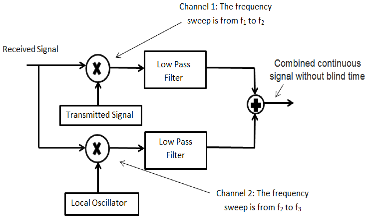
Figure 1: Receiver processing for DD-CTFM technique.

III Issues in DD-CTFM

In doing careful analysis of the DD-CTFM technique, it is found that there is a problem of phase discontinuity in the output signal. The output signal of DD-CTFM processing should ideally contain a sinusoidal waveform without any phase discontinuity, corresponding to each echo. However, there will be phase discontinuity in the concatenated sinusoids from the two channels as illustrated in Fig. 2.

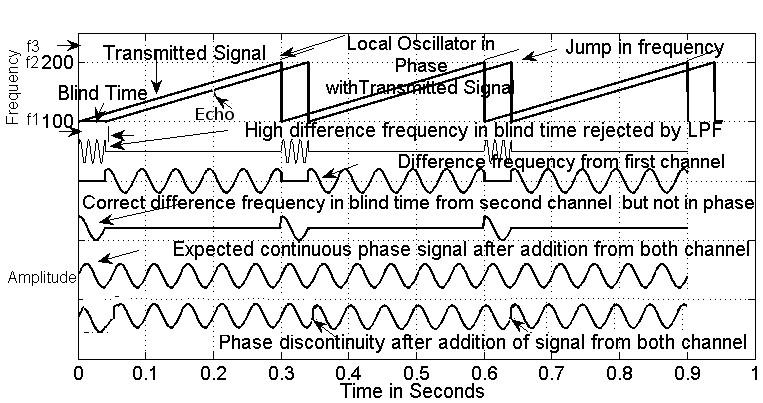
Figure 2: Time-frequency plot and DD-CTFM processing: difference between desired waveform (2^nd from bottom) and actual waveform (bottom).

The time-frequency plot and difference frequency signal waveforms are shown in Fig. 2. The upper part of Fig. 2 shows the time-frequency plots of the transmitted and received signals for a single target. The lower part of Fig. 2 shows the incorrect jump frequency (that does not contain the range information) and correct difference frequency signals respectively. The correct difference frequency signal refers to the desired signal corresponding to the actual delay. The jump difference frequency signal is incorrect as it contains wrong information of the delay. As shown in Fig. 2, the correct difference frequency signal is obtained from a segment of the total cycle duration only from channel 1. In the remaining part of each cycle just after the frequency jumps in the transmitted signal, the difference frequency signal becomes incorrect in channel 1. The duration for which we get the incorrect difference frequency signal is known as blind time and it depends on the target range. The blind time limits the total observation time of the correct frequency and hence limits the frequency resolution. To get the correct difference frequency signal during the blind time, a second channel with a local oscillator was proposed by Gough et al [1]. The desired added signal from both the channels is shown in Fig. 2 by the second last waveform, which does not contain any phase discontinuity. However, the actual concatenated sinusoids shown by the bottom waveform contains the phase discontinuity, which limits the observation time and hence the range resolution.

Mathematical explanation of phase discontinuity in the added signal

Let the transmitted signal $x(t)$ be a linear frequency modulated signal (up-chirp) represented as:

$$x(t)=cos\Big{(}2\pi(f_{1}t+\frac{\mu t^{2}}{2})\Big{)}$$ (1)

where $f_{1}$ represents the starting frequency of the LFM signal and $\mu$ is the sweep rate. Let $\phi_{x}(t)$ be the instantaneous phase of the transmitted signal given as:

$$\phi_{x}(t)=2\pi(f_{1}t+\frac{\mu t^{2}}{2}).$$ (2)

Let the received signal $y(t)$ be a delayed version of the transmitted signal given as:

$$y(t)=cos\Big{(}2\pi(f_{1}(t-\tau)+\frac{\mu}{2}(t-\tau)^{2})\Big{)}$$ (3)

where $\tau$ is the time delay of the received signal. The instantaneous phase of $y(t)$ be expressed as:

$$\phi_{y}(t)=2\pi(f_{1}(t-\tau)+\frac{\mu}{2}(t-\tau)^{2})$$ (4)

where $\phi_{y}(t)$ represents the phase of $y(t)$ at time $t$.

The transmitted and received signals are multiplied and low pass filtered in channel 1 as shown in Fig. 1. To get the ideally desired signal corresponding to a range cell during the blind time, a local oscillator is used. According to Gough et al [1] if the local oscillator is in phase continuity with the transmitted signal and with the same slope, we should get a continuous sinusoidal signal after the addition of the two channels. Let the local oscillator signal which is in phase continuity with the transmitted signal be given as:

$$z(t)=cos\Big{(}2\pi(f_{2}t+\frac{\mu}{2}t^{2})+\phi_{I}\Big{)}$$ (5)

where $f_{2}$ is the starting frequency of the local oscillator, that is equal to the final frequency of the transmitted chirp signal. The initial phase $\phi_{I}$ of the local oscillator is equal to the phase of the transmitted signal at the instant when the transmitted signal frequency reaches its final value. The initial phase $\phi_{I}$ is calculated using (2) as:

$$\phi_{I}=2\pi(f_{1}T+\frac{\mu}{2}T^{2}).$$ (6)

Let the phase of $z(t)$ be denoted by $\phi_{l}(t)$. It is given as:

$$\phi_{l}(t)=2\pi(f_{2}t+\frac{\mu}{2}t^{2})+\phi_{I}.$$ (7)

The phase of the low pass filtered signal at the output of channel 1 is calculated as:

$$\phi_{f1}(t)=\phi_{x}(t)-\phi_{y}(t).$$ (8)

The phase of the low pass filtered signal at the output of channel 2 is calculated as:

$$\phi_{f2}(t)=\phi_{l}(t)-\phi_{y}(t).$$ (9)

Let the starting frequency $f_{1}$, the final frequency $f_{2}$ and the duration $T$ of the chirp signal be taken as 100 Hz, 200 Hz and 300 ms respectively. Let the delay $\tau$ in the received signal be 93 ms. The value of $\mu$ for this case is 333.3 Hz/sec. The phase of the transmitted signal at $t=300$ ms using (2) is $(90\pi)_{mod2\pi}=0$ radians. The phase of the received signal at this instant using (4) is $(55.68)_{mod2\pi}=1.68\pi$ radians. So, the phase of the low pass filtered signal using (8) at $t=300$ ms from channel 1 is $(34.32\pi)_{mod2\pi}=0.32\pi$ radians. At $t=300$ ms, the transmitted signal will jump back to its starting frequency of 100 Hz for the next cycle. Now, the desired signal during the blind time is provided by channel 2. Using (4) and (7), the phase of the received signal $\phi_{y}$ and local oscillator signal $\phi_{l}$ at $t=300$ ms are $(55.68)_{mod2\pi}=1.68\pi$ and $(90\pi)_{mod2\pi}=0$ radians respectively. So, using (9) the starting phase of the low pass filtered signal from channel 2 is $(34.32\pi)_{mod2\pi}=0.32\pi$ radians. Thus, the phase of signals from the two channels is continuous without any discontinuity at $t=300$ ms.

At $t=393$ ms, the desired signal is obtained from channel 2. The phase of the local oscillator $\phi_{l}$ and the received signal $\phi_{y}$ at $t=393$ ms using (7) and (2), are $(130.08\pi)_{mod2\pi}=0.08\pi$ and $(90\pi)_{mod2\pi}=0$ radians respectively. So, the phase of the low pass filtered signal from channel 2 at the end of the first cycle using (9) is $(40.08\pi)_{mod2\pi}=0.08\pi$ radians. The desired signal just after $t=393$ ms is again obtained from channel 1. At $t=393$ ms in the next cycle, the phase of the transmitted $\phi_{x}$ and the received signals $\phi_{y}$ using (2) and (4), are $(21.48\pi)_{mod2\pi}=1.48\pi$ and $(90\pi)_{mod2\pi}=0$ radians respectively. The starting phase of channel 1 in the second cycle using (8) is $(-68.52\pi)_{mod2\pi}=-0.52\pi$ radians that is very different from the previous phase of $(40.08\pi)_{mod2\pi}=0.08\pi$. Thus, the added difference frequency signal from the two channels contains a strong phase discontinuity after $t=393$ ms. Thus, the observation duration of the sinusoidal signal corresponding to an echo is increased only by a duration equal to blind time, which is a fraction of total chirp duration. So, one cannot increase the observation duration to any desired value as claimed in [1]. The expressions for the phase of the two channels at various instants with a typical example explained above are summarized in table I to demonstrate the phase discontinuity issue.

Parameter	Expression	Example
Starting frequency	$f_{1}$	100 Hz
Final frequency of $x(t)$	$f_{2}$	200 Hz
Sweep duration	$T$	300 ms
Delay in $y(t)$	$\tau$	93 ms
Sweep rate	$\dfrac{(f_{2}-f_{1})}{T}$	333.3 Hz/sec.
Phase of $x(t)$ at $t=T$	$\phi_{x}(t)=2\pi(f_{1}T+\dfrac{\mu}{2}T^{2})$	90$\pi$
Phase of $y(t)$ at $t=T$	$\phi_{y}(t)=2\pi(f_{1}(T-\tau)+\dfrac{\mu}{2}(T-\tau)^{2})$	55.68$\pi$
Phase of $z(t)$ at $t=T$	$\phi_{l}(t)=\phi_{i}$	90$\pi$
Phase of $x(t)$	$\phi_{x}(t)=2\pi(f_{1}\tau+\dfrac{\mu}{2}\tau^{2})$	40.08$\pi$
at $t=T+\tau$
Phase of $y(t)$	$\phi_{y(t)}=2\pi(f_{1}T+\dfrac{\mu}{2}T^{2})$	90$\pi$
at $t=T+\tau$
Phase of $z(t)$	$\phi_{l}(t)=2\pi(f_{2}\tau+\dfrac{\mu}{2}\tau^{2})+\phi_{i}$	130.08$\pi$
at $t=T+\tau$
Phase of	$\phi_{f2}(t)=\phi_{x}(t)-\phi_{y}(t)$	34.32$\pi$
channel 1 at $t=T$
Phase of	$\phi_{f2}(t)=\phi_{l}(t)-\phi_{y}(t)$	34.32$\pi$
channel 2 at $t=T$
Phase of channel 1	$\phi_{f2}(t)=\phi_{x}(t)-\phi_{y}(t)$	-49.92$\pi$
at $t=T+\tau$
Phase of channel 2	$\phi_{f2}(t)=\phi_{l}(t)-\phi_{y}(t)$	40.08$\pi$
at $t=T+\tau$

TABLE I: Parameters for calculation of phase mismatch in DD-CTFM processing.

Simulation study of phase discontinuity in the added signal

For the simulation study the parameters starting frequency $f_{1}$, final frequency $f_{2}$ and duration $T$ of the chirp signal are taken to be 100 Hz, 200 Hz and 300 ms respectively. The parameters starting frequency $f_{2}$, final frequency $f_{3}$ and duration $T$ of the chirp signal generated using local oscillator are taken to be 200 Hz, 240 Hz and 120 ms respectively. The number of sweep cycles are taken to be 12, so the output signal duration is 3.6 seconds. The maximum duration of blind time is assumed to be 120 ms. The initial phase of the transmitted chirp signal is taken as 0. The initial phase of the local oscillator is taken to be same as the phase of the transmitted chirp signal at 300 ms. Let the received signal consist of a delayed version of the transmitted signal. Let the delay in the received signal be 96 ms. So, the DD-CTFM output frequency in this simulation should ideally be 32 Hz. However, it is estimated as 31.01 Hz as observed from Fig. 3 for this simulated case. Due to phase discontinuities in every sweep of the chirp signal, the observation time is still limited just as in case of CTFM processing and hence there will be an error in the estimate of the correct difference frequency. Thus, the range resolution improvement in DD-CTFM technique is only slightly better depending upon the blind time duration compared to $\frac{C}{2\bigtriangleup f}$ of CTFM technique. This improvement is negligible compared to the claim made in [1] which states that “the output will be truly continuous resulting in the complete elimination of the blind time and in a range resolution as good as two wavelengths of the mean frequency”.

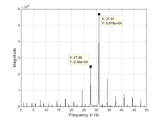
Figure 3: DFT magnitude plot of the output signal in DD-CTFM processing with phase discontinuity problem.

Sidelobe artifact issue

There is another issue of sidelobe artifacts in the DFT magnitude of the DD-CTFM output signal. The artifacts are located at integer multiples of $\dfrac{1}{T}$ Hz around the estimated frequency in the form of peaks at several bins in DFT of the DD-CTFM output signal. For the simulation example, the side lobe artifacts exist at integer multiples of $3.33$ Hz as shown in Fig. 3, from $31.01$ Hz . The side lobe artifacts are only 2.3 times i.e., 7.26 dB down the main peak as shown in Fig. 3. Thus, another weaker target echo with amplitude up to 7.26 dB below the main echo magnitude, will not be detected.

IV Conclusion

The issues in DD-CTFM technique proposed by Gough et al [1] are presented. The mathematical analysis and simulation example demonstrate the incorrect inference of DD-CTFM technique which states that which states that “we have managed to eliminate the blind time associated with conventional CTFM sonars, thus making the output truly continuous” [1].

References

- [1] A. d. R. P. T. Gough and M. J. Cusdin, “Continuous transmission FM sonar with one octave bandwidth and no blind time,” Proceedings of the IEE, vol. F-131, pp. 270-74, June 1984.
- [2] Z. Politis, P.J. Probert, “Target localization and identification using CTFM sonar imaging:the AURBIT method,” IEEE International Symposium on Computational Intelligence in Robotics ans Automation, pp. 256-261, Nov. 1999.
- [3] A. G. Stove, “Linear FMCW Radar Techniques,” IEE Proceedings-F, Vol. 139, No. 5, October 1992, pp. 343- 350.