Quantum phases of a two-dimensional polarized degenerate Fermi gas in an optical cavity

Abstract

In this paper we analytically investigate the ground-state properties of a two-dimensional polarized degenerate Fermi gas in a high-finesse optical cavity, which is governed by a generalized Fermi-Dicke model with tunable parameters. By solving the photon-number dependent Bogoliubov–de–Gennes equation, we find rich quantum phases and phase diagrams, which depend crucially on the fermion-photon coupling strength, the fermion-fermion interaction strength, and the atomic resonant frequency (effective Zeeman field). In particular, without the fermion-fermion interaction and with a weak atomic resonant frequency, we find a mixed phase that the normal phase with two Fermi surfaces and the superradiant phase coexist, and reveal a first-order phase transition from this normal phase to the superradiant phase. With the intermediate fermion-fermion interaction and fermion-photon coupling strengths, we predict another mixed phase that the superfluid and superradiant phases coexist. Finally, we address briefly how to detect these predicted quantum phases and phase diagrams in experiments.

I Introduction

The experimental combination of a Bose-Einstein condensate with a high-finesse optical cavity FB07 ; YC07 opens a conceptually new regime of both cavity quantum electrodynamics and ultracold atoms. In this combination, all ultracold bosons, occupying the same quantum state, interact identically with a single-mode quantized field, and thus, a strong collective matter-field interaction can be achieved. Moreover, cavities can generate unconventional dynamical optical potentials, which induce rich nonequilibrium and strongly-corrected many-body phenomena HR13 . For example, when pumped transversely, the spinless ultracold bosons in the cavity-induced dynamical optical potentials undergo self-organization PD02 ; DN06 ; DN08 , which has been observed experimentally KB10 ; KB11 and has been regarded as an equivalence to the well-known superradiant (SR) phase transition in an effective Dicke model DH54 .

Motivated by near-term experimental prospects, another fundamental interaction between ultracold fermions and a high-finesse optical cavity has been investigated theoretically. Since at lower temperature fermions exhibit quite different behavior than bosons, exotic physics is expected to arise in this new platform RK10 ; QS11 ; MM12 ; XG12 ; BP13 ; JK14 ; FP14 ; YC14 ; JP14 ; YC15 ; CK16 ; AS16 ; ASF16 ; WZ16 . In particular, followed by the experimental scheme in Ref. KB10 ; KB11 , three groups have considered simultaneously spinless fermions in the cavity-induced dynamical optical potential JK14 ; FP14 ; YC14 . They have found that the Fermi statistics plays a dominate role in the SR phase transition at moderate and high densities. At the moderate density, the Fermi surface displays a nesting structure and strongly enhances superradiance, which is, however, suppressed largely at high density, due to the Pauli blocking effect. In addition, by introducing a cavity-assisted spin-orbit coupling YD14 ; LD14 , a topological SR phase has been predicted JP14 . Recently, the cavity-induced artificial magnetic field CK16 , chiral phases AS16 , and non-trivial topological states ASF16 have been created. Moreover, when fermions are gauge coupled to a cavity mode, a SR phase with an infinitesimal pumping threshold, which induces a directed particle flow, has been found for an infinite lattice WZ16 .

In this paper, followed by the experimental scheme in Ref. KJA12 ; MPB14 , we consider a two-dimensional (2D) polarized degenerate Fermi gas in a high-finesse optical cavity. When introducing two Raman transitions induced by the quantized cavity field and two transverse pumping lasers, we first realize a generalized Fermi-Dicke model, in which all parameters, including the fermion-photon coupling strength, the fermion-fermion interaction strength, and the atomic resonant frequency (effective Zeeman field), can be controlled independently. Then, based on a photon-number dependent Bogoliubov–de–Gennes (BdG) equation, we reveal rich quantum phases and phase diagrams, which depend crucially on these tunable parameters. In particular, without the fermion-fermion interaction and with a weak atomic resonant frequency, we find a mixed phase that the normal phase with two Fermi surfaces and the SR phase coexist, and reveal a first-order phase transition from this normal phase to the SR phase. With the intermediate fermion-fermion interaction and fermion-photon coupling strengths, we predict another mixed phase that the superfluid (SF) and SR phases coexist. Finally, we address briefly how to detect the predicted quantum phases and phase diagrams in experiments.

This paper is organized as follows. In Sec. II, we present an experimentally-feasible scheme to realize a generalized Fermi-Dicke model with tunable parameters. In Sec. III, we derive a photon-number dependent BdG equation, and then obtain the ground-state energy and the mean-field gap, particle number, and SR equations. In Secs. IV and V, we reveal rich quantum phases and phase diagrams without or with the fermion-fermion two-body interaction, respectively. The parameter estimation and possible experimental observation are addressed in Sec. VI, and the brief discussion and conclusion are given in Sec. VII.

II Model and Hamiltonian

Figure 1 shows our proposed scheme that all ultracold fermions are coupled with a high-finesse optical cavity supporting a single-mode photon. As illustrated in Fig. 1(a), the fermions in the optical cavity are confined in a far-of-resonance optical trap ($yz$ plane) by a tightly-radial confinement along the $x$ direction. The cavity mode is driven by a linearly-polarized laser and the fermions are pumped by two transverse lasers, which are left- and right-handed circular polarized in the $yz$ plane. In addition, each fermion has four levels, including two ground states ($\left|\uparrow\right\rangle$ and $\left|\downarrow\right\rangle$) and two excited states ($\left|1\right\rangle$ and $\left|2\right\rangle$), as shown in Fig. 1(b). The quantized cavity field and the two transverse pumping lasers induce two Raman processes; see more details in the caption.

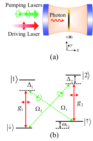
Figure 1: (a) Our proposed schematic setup that all ultracold fermions (black online), which are confined in a far-of-resonance optical trap (yellow online) of the $yz$ plane by a tightly-radial confinement along the $x$ direction, are coupled with a high-finesse optical cavity. The cavity mode is driven by a linearly-polarized driving laser (with frequency $\omega_{l}$), which propagates along the $x$ direction. Two transverse pumping lasers (with frequencies $\omega_{A}$ and $\omega_{B}$), which are left- and right-handed circular polarized in the $yz$ plane, propagate along the $x$ direction and induce two Raman processes by combining the quantized cavity field. In order to obtain a time-independent Hamiltonian, these frequencies should satisfy the following condition: $\omega_{l}=\left(\omega_{A}+\omega_{B}\right)/2$; see the detailed derivation in the main text. The magnetic field $\mathbf{B}$ is applied along the positive $z$ direction and produces a Zeeman shift between two hyperfine ground states. (b) The atomic energy levels and their transitions. Each fermion has two ground states ($\left|\uparrow\right\rangle$ and $\left|\downarrow\right\rangle$) and two excited states ($\left|1\right\rangle$ and $\left|2\right\rangle$). The $\left|\downarrow\right\rangle$ $\longleftrightarrow\left|1\right\rangle$ and $\left|\uparrow\right\rangle$ $\longleftrightarrow\left|2\right\rangle$ transitions (red solid lines) are caused by the quantized cavity field with fermion-photon coupling strengths $g_{1}$ and $g_{2}$. The $\left|\uparrow\right\rangle$ $\longleftrightarrow\left|1\right\rangle$ and $\left|\downarrow\right\rangle$ $\longleftrightarrow\left|2\right\rangle$ transitions (green dashed lines) are governed by the transverse pumping lasers with Rabi frequencies $\Omega_{1}$ and $\Omega_{2}$. $\omega_{\uparrow\downarrow}=\omega_{\uparrow}-\omega_{\downarrow}$ is the resonant frequency between the ground states $\left|\uparrow\right\rangle$ and $\left|\downarrow\right\rangle$ with eigenfrequencies $\omega_{\uparrow}$ and $\omega_{\downarrow}$. $\Delta_{1}$ and $\Delta_{2}$ are the detunings from the excited states $\left|1\right\rangle$ and $\left|2\right\rangle$.

Formally, the total time-dependent 2D Hamiltonian is written as

$$\hat{H}_{\text{T}}(t)=\hat{H}_{\text{F}}+\hat{H}_{\text{P}}+\hat{H}_{\text{D}}(t)+\hat{H}_{\text{AR}}(t)+\hat{H}_{\text{AP}}+\hat{H}_{\text{INT}}.$$ (1)

Here, the Hamiltonian of the free four-level fermions is given by

$$\hat{H}_{\text{F}}=\sum_{i=1,2,\uparrow,\downarrow}\int d^{2}\mathbf{r}\hat{\psi}_{i}^{\dagger}\left(\mathbf{r}\right)\left(\frac{\mathbf{\hat{p}}^{2}}{2M}-\mu+\omega_{i}\right)\hat{\psi}_{i}\left(\mathbf{r}\right),$$ (2)

where $\hat{\psi}_{i}^{\dagger}\left(\mathbf{r}\right)$ and $\hat{\psi}_{i}\left(\mathbf{r}\right)$ ($i=1,2,\downarrow,\uparrow$) are the creation and annihilation operators of the fermionic fields, $M$ is the atom mass, $\mu$ is the chemical potential, and $\omega_{i}$ are the eigenfrequencies of all quantum states. The Hamiltonian of the quantized cavity field, together with the driving laser, is written as

$$\hat{H}_{\text{P}}+\hat{H}_{\text{D}}(t)=\omega_{c}\hat{a}^{{\dagger}}\hat{a}+\varepsilon\left(\hat{a}e^{i\omega_{l}t}+\hat{a}^{\dagger}e^{-i\omega_{l}t}\right),$$ (3)

where $\hat{a}^{{\dagger}}$ and $\hat{a}$ are the creation and annihilation operators of the quantized cavity field with frequency $\omega_{c}$, and $\varepsilon$ ($\omega_{l}$) is the magnitude (frequency) of the driving laser. Under the rotating-wave approximation, the Hamiltonian, which describes the interaction between the fermionic fields and the two transverse pumping lasers, reads

$$\hat{H}_{\text{AR}}(t) = \frac{1}{2}\int d^{2}\mathbf{r}\left[\Omega_{1}\hat{\psi}_{1}^{\dagger}\left(\mathbf{r}\right)\hat{\psi}_{\uparrow}\left(\mathbf{r}\right)e^{-i\omega_{A}t}\right.$$ (4)

$$+\left.\Omega_{2}\hat{\psi}_{2}^{\dagger}\left(\mathbf{r}\right)\hat{\psi}_{\downarrow}\left(\mathbf{r}\right)e^{-i\omega_{B}t}+\text{H.c.}\right],$$

where $\Omega_{1}$ and $\Omega_{2}$ ($\omega_{A}$ and $\omega_{B}$) are the Rabi frequencies (frequencies) of the transverse pumping lasers and H.c. denotes the Hermitian conjugate, whereas the Hamiltonian for governing the interaction between the fermionic and quantized cavity fields is given by

$$\hat{H}_{\text{AP}}\!=\!\!\int\!d^{2}\mathbf{r}\left\{\left[g_{1}\hat{\psi}_{1}^{\dagger}\left(\mathbf{r}\right)\hat{\psi}_{\downarrow}\left(\mathbf{r}\right)\!+\!g_{2}\hat{\psi}_{2}^{\dagger}\left(\mathbf{r}\right)\hat{\psi}_{\uparrow}\left(\mathbf{r}\right)\right]\hat{a}\!+\!\text{H.c.}\!\right\},$$ (5)

where $g_{1}$ and $g_{2}$ are both the fermion-photon coupling strengths. In addition, here we only consider the attractive contact interaction between the ground states $\left|\uparrow\right\rangle$ and $\left|\downarrow\right\rangle$ since the excited states are eliminated adiabatically, as will be shown below. Therefore, the two-body interacting Hamiltonian is given by

$$\hat{H}_{\text{INT}}=\lambda\int d^{2}\mathbf{r}\hat{\psi}_{\uparrow}^{\dagger}\left(\mathbf{r}\right)\hat{\psi}_{\downarrow}^{\dagger}\left(\mathbf{r}\right)\hat{\psi}_{\downarrow}\left(\mathbf{r}\right)\hat{\psi}_{\uparrow}\left(\mathbf{r}\right),$$ (6)

where $\lambda$ is the negative interaction strength, i.e., $\lambda\;<\;0$.

For the time-dependent Hamiltonian (1), we first perform a unitary transformation $\hat{U}(t)=\exp\left(i\hat{H}^{\prime}t\right)$, where

$$\hat{H}^{\prime} = \omega_{l}\hat{a}^{{\dagger}}\hat{a}+\frac{\omega_{B}}{2}\left[\hat{\psi}_{2}^{\dagger}\left(\mathbf{r}\right)\hat{\psi}_{2}\left(\mathbf{r}\right)-\hat{\psi}_{\downarrow}^{\dagger}\left(\mathbf{r}\right)\hat{\psi}_{\downarrow}\left(\mathbf{r}\right)\right]$$ (7)

$$+\frac{\omega_{A}}{2}\left[\hat{\psi}_{1}^{\dagger}\left(\mathbf{r}\right)\hat{\psi}_{1}\left(\mathbf{r}\right)-\hat{\psi}_{\uparrow}^{\dagger}\left(\mathbf{r}\right)\hat{\psi}_{\uparrow}\left(\mathbf{r}\right)\right]$$

with $\omega_{l}=\left(\omega_{B}+\omega_{A}\right)/2$, to obtain a time-independent Hamiltonian $\hat{H}_{1}=\hat{U}(t)\hat{H}_{\text{T}}(t)\hat{U}^{\dagger}(t)+i\left[\partial\hat{U}(t)/\partial t\right]\hat{U}^{\dagger}(t)$, i.e.,

$$\hat{H}_{1} = \tilde{\omega}\hat{a}^{{\dagger}}\hat{a}+\varepsilon\left(\hat{a}+\hat{a}^{\dagger}\right)+\sum_{i=1,2,\uparrow,\downarrow}\int d^{2}\mathbf{r}\hat{\psi}_{i}^{\dagger}\left(\mathbf{r}\right)\left(\frac{\mathbf{\hat{p}}^{2}}{2M}-\mu\right)\hat{\psi}_{i}\left(\mathbf{r}\right)+\int d^{2}\mathbf{r}\left[\Delta_{1}\hat{\psi}_{1}^{\dagger}\left(\mathbf{r}\right)\hat{\psi}_{1}\left(\mathbf{r}\right)+\Delta_{2}\hat{\psi}_{2}^{\dagger}\left(\mathbf{r}\right)\hat{\psi}_{2}\left(\mathbf{r}\right)\right]$$ (8)

$$+\int d^{2}\mathbf{r}\left[\tilde{\omega}_{\uparrow}\hat{\psi}_{\uparrow}^{\dagger}\left(\mathbf{r}\right)\hat{\psi}_{\uparrow}\left(\mathbf{r}\right)+\tilde{\omega}_{\downarrow}\hat{\psi}_{\downarrow}^{\dagger}\left(\mathbf{r}\right)\hat{\psi}_{\downarrow}\left(\mathbf{r}\right)\right]+\frac{1}{2}\int d^{2}\mathbf{r}\left[\Omega_{1}\hat{\psi}_{1}^{\dagger}\left(\mathbf{r}\right)\hat{\psi}_{\uparrow}\left(\mathbf{r}\right)+\Omega_{2}\hat{\psi}_{2}^{\dagger}\left(\mathbf{r}\right)\hat{\psi}_{\downarrow}\left(\mathbf{r}\right)+\text{H.c.}\right]$$

$$+\lambda\int d^{2}\mathbf{r}\hat{\psi}_{\uparrow}^{\dagger}\left(\mathbf{r}\right)\hat{\psi}_{\downarrow}^{\dagger}\left(\mathbf{r}\right)\hat{\psi}_{\downarrow}\left(\mathbf{r}\right)\hat{\psi}_{\uparrow}\left(\mathbf{r}\right)+\int d^{2}\mathbf{r}\left\{\left[g_{1}\hat{\psi}_{1}^{\dagger}\left(\mathbf{r}\right)\hat{\psi}_{\downarrow}\left(\mathbf{r}\right)+g_{2}\hat{\psi}_{2}^{\dagger}\left(\mathbf{r}\right)\hat{\psi}_{\uparrow}\left(\mathbf{r}\right)\right]\hat{a}+\text{H.c.}\right\}.$$

where $\tilde{\omega}=\omega_{c}-\omega_{l}$ is the effective cavity frequency, $\Delta_{1}=\omega_{1}-\omega_{A}/2$ ($\Delta_{2}=\omega_{2}-\omega_{B}/2$) is the detuning from the excited state $\left|1\right\rangle$ ($\left|2\right\rangle$), and $\tilde{\omega}_{\uparrow}=$ $\omega_{\uparrow}+\omega_{A}/2$ ($\tilde{\omega}_{\downarrow}=\omega_{\downarrow}+\omega_{B}/2$) is the effective eigenfrequency of the ground state $\left|\uparrow\right\rangle$ ($\left|\downarrow\right\rangle$).

In experiments KB10 ; KB11 ; MPB14 , a weak driving ($\varepsilon\rightarrow 0$) and large detunings ($\left|\Delta_{1,2}\right|\gg\left\{\Omega_{1,2},g_{1,2},\tilde{\omega},\omega_{0}\right\}$) are usually taken into account. In such case, the term $\varepsilon\left(a+a^{\dagger}\right)$ in the Hamiltonian (8) can be neglected and both the excited states $\left|1\right\rangle$ and $\left|2\right\rangle$ can be eliminated adiabatically FD07 ; JF14 . Therefore, we obtain

$$\hat{H} = \tilde{\omega}\hat{a}^{{\dagger}}\hat{a}+\sum_{\sigma=\uparrow,\downarrow}\int d^{2}\mathbf{r}\hat{\psi}_{\sigma}^{\dagger}\left(\mathbf{r}\right)\left(\frac{\mathbf{p}^{2}}{2M}-\mu\right)\hat{\psi}_{\sigma}\left(\mathbf{r}\right)+\int d^{2}\mathbf{r}\left[\tilde{\omega}_{\uparrow}\hat{\psi}_{\uparrow}^{\dagger}\left(\mathbf{r}\right)\hat{\psi}_{\uparrow}\left(\mathbf{r}\right)+\tilde{\omega}_{\downarrow}\hat{\psi}_{\downarrow}^{\dagger}\left(\mathbf{r}\right)\hat{\psi}_{\downarrow}\left(\mathbf{r}\right)\right]$$ (9)

$$+\lambda\int d^{2}\mathbf{r}\hat{\psi}_{\uparrow}^{\dagger}\left(\mathbf{r}\right)\hat{\psi}_{\downarrow}^{\dagger}\left(\mathbf{r}\right)\hat{\psi}_{\downarrow}\left(\mathbf{r}\right)\hat{\psi}_{\uparrow}\left(\mathbf{r}\right)+\int d^{2}\mathbf{r}\left[\frac{|g_{2}|^{2}}{\Delta_{2}}\hat{\psi}_{\uparrow}^{\dagger}\left(\mathbf{r}\right)\hat{\psi}_{\uparrow}\left(\mathbf{r}\right)+\frac{|g_{1}|^{2}}{\Delta_{1}}\hat{\psi}_{\downarrow}^{\dagger}\left(\mathbf{r}\right)\hat{\psi}_{\downarrow}\left(\mathbf{r}\right)\right]\hat{a}^{\dagger}\hat{a}$$

$$+\frac{1}{2}\int d^{2}\mathbf{r}\left\{\left[\frac{g_{2}\Omega_{2}^{\ast}}{\Delta_{2}}\hat{\psi}_{\downarrow}^{\dagger}\left(\mathbf{r}\right)\hat{\psi}_{\uparrow}\left(\mathbf{r}\right)+\frac{g_{1}\Omega_{1}^{\ast}}{\Delta_{1}}\hat{\psi}_{\uparrow}^{\dagger}\left(\mathbf{r}\right)\hat{\psi}_{\downarrow}\left(\mathbf{r}\right)\right]\hat{a}+\text{H.c.}\right\}.$$

When the parameters are chosen as

$$\frac{|g_{1}|^{2}}{\Delta_{1}}=\frac{|g_{2}|^{2}}{\Delta_{2}}\text{, \ \ \ \ }\frac{g_{1}\Omega_{1}^{\ast}}{\Delta_{1}}=\frac{g_{2}\Omega_{2}^{\ast}}{\Delta_{2}},$$ (10)

the Hamiltonian (9) becomes

$$\hat{H} = \omega\hat{a}^{{\dagger}}\hat{a}+\sum_{\sigma=\uparrow,\downarrow}\int d^{2}\mathbf{r}\hat{\psi}_{\sigma}^{\dagger}\left(\mathbf{r}\right)\left(\frac{\mathbf{\hat{p}}^{2}}{2M}-\mu\right)\hat{\psi}_{\sigma}\left(\mathbf{r}\right)$$ (11)

$$-\omega_{0}\int d^{2}\mathbf{r}\left[\hat{\psi}_{\uparrow}^{\dagger}\left(\mathbf{r}\right)\hat{\psi}_{\uparrow}\left(\mathbf{r}\right)-\hat{\psi}_{\downarrow}^{\dagger}\left(\mathbf{r}\right)\hat{\psi}_{\downarrow}\left(\mathbf{r}\right)\right]$$

$$+\frac{\eta}{\sqrt{N}}\int d^{2}\mathbf{r}\left[\hat{\psi}_{\downarrow}^{\dagger}\left(\mathbf{r}\right)\hat{\psi}_{\uparrow}\left(\mathbf{r}\right)+\hat{\psi}_{\uparrow}^{\dagger}\left(\mathbf{r}\right)\hat{\psi}_{\downarrow}\left(\mathbf{r}\right)\right]\left(\hat{a}+\hat{a}^{\dagger}\right)$$

$$+\lambda\int d^{2}\mathbf{r}\hat{\psi}_{\uparrow}^{\dagger}\left(\mathbf{r}\right)\hat{\psi}_{\downarrow}^{\dagger}\left(\mathbf{r}\right)\hat{\psi}_{\downarrow}\left(\mathbf{r}\right)\hat{\psi}_{\uparrow}\left(\mathbf{r}\right),$$

where the factor $1/\sqrt{N}$, with $N$ being the total atom number, is introduced to ensure that the free energy per fermion is finite in the thermodynamic limit YKW73 ; FTH73 . In the Hamiltonian (11), $\omega_{0}=$ $\left(\tilde{\omega}_{\downarrow}-\tilde{\omega}_{\uparrow}\right)/2$ is the effective resonant frequency between the ground states $\left|\uparrow\right\rangle$ and $\left|\downarrow\right\rangle$ and can be usually regarded as an effective Zeeman field. For simplicity, we take $\omega_{0}>0$ in the following discussions. $\eta=\sqrt{N}g_{1}\Omega_{1}^{\ast}/\left(2\Delta_{1}\right)$ $=\sqrt{N}g_{2}\Omega_{2}^{\ast}/\left(2\Delta_{2}\right)$ is the effective fermion-photon coupling strength. $\omega=N\zeta+\tilde{\omega}$ is the atom-number dependent cavity frequency, where $\zeta=|g_{1}|^{2}/\Delta_{1}=|g_{2}|^{2}/\Delta_{2}$. It should be emphasized that the choice of parameters in Eq. (10) has been used experimentally KB10 ; KB11 ; MPB14 .

The Hamiltonian (11) is our required Hamiltonian that governs two fundamental interactions, including the fermion-photon and fermion-fermion two-body interactions, and thus, is called a generalized Fermi-Dicke model. This Hamiltonian has a distinct advantage that all parameters can be controlled independently. For example, $\omega_{0}$ and $\omega$ can be tuned by controlling the frequencies of the driving and transverse pumping lasers, and $\eta$ can be determined by the Rabi frequencies of the transverse pumping lasers. Besides, $\lambda$ can be tuned by varying the $s$-wave scattering length $a_{s}$ through the Feshbach resonant technique CC10 . See more detailed discussions in Sec. VI.

III Ground-state properties

In order to investigate the ground-state properties of the Hamiltonian (11), we first expand operators of the fermionic fields in terms of the plane waves, i.e.,

$$\hat{\psi}_{\sigma}\left(\mathbf{r}\right)=\frac{1}{\sqrt{S}}\sum_{\mathbf{k,}\sigma=\uparrow,\downarrow}\hat{C}_{\mathbf{k},\sigma}e^{i\mathbf{k\cdot r}},$$ (12)

where $\hat{C}_{\mathbf{k},\sigma}$ are the annihilation operators of fermions in the momentum space and $S$ is the gas area (hereafter $S=1$). After a straightforward calculation, we obtain

$$\hat{H} = \omega\hat{a}^{{\dagger}}\hat{a}+\sum_{\mathbf{k}}\xi_{\mathbf{k}}\hat{C}_{\mathbf{k},\sigma}^{\dagger}\hat{C}_{\mathbf{k},\sigma}+\omega_{0}\sum_{\mathbf{k}}\left(\hat{C}_{\mathbf{k},\uparrow}^{\dagger}\hat{C}_{\mathbf{k},\uparrow}-\hat{C}_{\mathbf{k},\downarrow}^{\dagger}\hat{C}_{\mathbf{k},\downarrow}\right)$$ (13)

$$+\lambda\sum_{\mathbf{k}}\hat{C}_{\mathbf{k},\uparrow}^{\dagger}\hat{C}_{-\mathbf{k},\downarrow}^{\dagger}\hat{C}_{-\mathbf{k},\downarrow}\hat{C}_{\mathbf{k},\uparrow}+\frac{\eta}{\sqrt{n}}\sum_{\mathbf{k}}\left(\hat{C}_{\mathbf{k},\uparrow}^{\dagger}\hat{C}_{\mathbf{k},\downarrow}+\hat{C}_{\mathbf{k},\downarrow}^{\dagger}\hat{C}_{\mathbf{k},\uparrow}\right)\left(\hat{a}+\hat{a}^{\dagger}\right),$$

where $\xi_{\mathbf{k}}=\epsilon_{\mathbf{k}}-\mu$, $\epsilon_{\mathbf{k}}=\mathbf{k}^{2}/2M$ is the kinetic energy, $n=K_{F}^{2}/\left(2\pi\right)=E_{F}M/\pi$ is the density of fermions in 2D, and $E_{F}=K_{F}^{2}/\left(2M\right)$ is the Fermi energy. The Hamiltonian (13) describes the interaction between two-component ultracold fermions and a high-finesse optical cavity in the momentum space.

For the attractive fermion-fermion two-body interaction, the Cooper pairing with the opposite momentum and different spin is formed near to the Fermi surface LNC56 . In the mean-field approximation, the corresponding SF order parameter called the gap is assumed as MR89 ; MR90

$$\Delta=\lambda\sum_{\mathbf{k}}\left\langle\hat{C}_{-\mathbf{k},\downarrow}\hat{C}_{\mathbf{k},\uparrow}\right\rangle.$$ (14)

In such case, the two-body interacting Hamiltonian becomes

$$\hat{H}_{\text{INT}}=\Delta\sum_{\mathbf{k}}\left(\hat{C}_{-\mathbf{k},\downarrow}\hat{C}_{\mathbf{k},\uparrow}+\hat{C}_{\mathbf{k},\uparrow}^{\dagger}\hat{C}_{-\mathbf{k},\downarrow}^{\dagger}\right)-\frac{\Delta^{2}}{\lambda}.$$ (15)

For simplicity, the mean-field gap is here assumed to be real, i.e., $\Delta=\Delta^{\ast}$.

In addition, our considered system usually exists the cavity decay with rate $\kappa$, and thus, we should introduce the Hesienberg-Langevin equation for the cavity field operator $\hat{a}$ GWF88 ; MOS97 ,

$$i\frac{\partial\hat{a}}{\partial t}=\left[\hat{a},\hat{H}\right]-i\kappa\hat{a}+\hat{\gamma}_{\text{in}}\left(t\right),$$ (16)

where $\hat{\gamma}_{\text{in}}\left(t\right)$ is the quantum noise operator and satisfies the following conditions: $\left\langle\hat{\gamma}_{\text{in}}^{\dagger}\left(t\right)\hat{\gamma}_{\text{in}}\left(t^{\prime}\right)\right\rangle=2\kappa\delta\left(t-t^{\prime}\right)$ and $\left\langle\hat{\gamma}_{\text{in}}\left(t\right)\hat{\gamma}_{\text{in}}\left(t^{\prime}\right)\right\rangle=0$. In general, the fluctuation of quantum noise varies faster than $1/\kappa$ on the time scale JL08 . When the time scale of the atom dynamics in the motional degree of freedom is larger than $1/\kappa$, the cavity field can reach a steady state DN08 ; KB10 , which is responsible for obtaining the ground-state phase diagrams. In terms of Eqs. (13) and (16), the steady-state solution of $\hat{a}$ is given by

$$\alpha=\left\langle\hat{a}\right\rangle=\frac{\eta\sum_{k}\left\langle\hat{C}_{\mathbf{k},\uparrow}^{\dagger}\hat{C}_{\mathbf{k},\downarrow}+\hat{C}_{\mathbf{k},\downarrow}^{\dagger}\hat{C}_{\mathbf{k},\uparrow}\right\rangle}{\sqrt{n}\left(-\omega+i\kappa\right)}.$$ (17)

Notice that when considering $\left\langle\hat{a}\right\rangle$, the noise term can be neglected. In experiments KB10 ; KB11 , the mean-photon number $\left\langle\hat{a}^{\dagger}\hat{a}\right\rangle=\left|\alpha\right|^{2}$ governs the SR properties and is thus called the SR order parameter.

Based on above discussions and in the basis of Nambu spinor $\hat{\Psi}_{\mathbf{k}}=\left(\hat{C}_{\mathbf{k},\uparrow},\hat{C}_{\mathbf{k},\downarrow},\hat{C}_{-\mathbf{k},\downarrow}^{\dagger},-\hat{C}_{-\mathbf{k},\uparrow}^{\dagger}\right)^{T}$, where $T$ stands for the transposition of a matrix, the Hamiltonian (13) turns into

$$\hat{H}=\frac{1}{2}\sum_{\mathbf{k}}\hat{\Psi}_{\mathbf{k}}^{\dagger}M_{\mathbf{k}}\hat{\Psi}_{\mathbf{k}}+\sum_{\mathbf{k}}\xi_{\mathbf{k}}-\frac{\Delta^{2}}{\lambda}+\omega\left|\alpha\right|^{2},$$ (18)

where the photon-number dependent BdG matrix is given by

$$M_{\mathbf{k}}=\left(\begin{array}[]{cccc}\xi_{\mathbf{k}}-\omega_{0}&\bar{\eta}&\Delta&0\\ \bar{\eta}&\xi_{\mathbf{k}}+\omega_{0}&0&\Delta\\ \Delta&0&-\xi_{\mathbf{k}}-\omega_{0}&\bar{\eta}\\ 0&\Delta&\bar{\eta}&-\xi_{\mathbf{k}}+\omega_{0}\end{array}\right),$$ (19)

with $\bar{\eta}=\eta\left(\alpha+\alpha^{\ast}\right)/\sqrt{n}$. The BdG matrix (19) is also written as

$$M_{\mathbf{k}}=\left(\begin{array}[]{cc}H_{0}&\Delta\mathbbm{1}\\ \Delta\mathbbm{1}&-\sigma_{y}H_{0}\sigma_{y}\end{array}\right),$$ (20)

where $H_{0}=\xi_{\mathbf{k}}+\omega_{0}\sigma_{z}+\bar{\eta}\sigma_{x}$, $\sigma_{x}$ and $\sigma_{y}$ are the Pauli matrices, and $\mathbbm{1}$ is the $2\times 2$ unit matrix. The property of the BdG matrix (20) implies that the Hamiltonian (18) has the particle-hole symmetry.

By diagonalizing the BdG matrix $M_{\mathbf{k}}$, we obtain the following dispersion relations of the Bogoliubov quasiparticles:

$$E_{\mathbf{k},\pm}^{\upsilon}=\upsilon\left(\sqrt{\xi_{\mathbf{k}}^{2}+\Delta^{2}}\pm\sqrt{\bar{\eta}^{2}+\omega_{0}^{2}}\right),$$ (21)

where $\upsilon=\pm 1$ correspond to the particle and hole branches of the excitation spectra, and $\bar{\eta}^{2}=4\omega^{2}\eta^{2}\left|\alpha\right|^{2}/\left[n\left(\omega^{2}+\kappa^{2}\right)\right]$. For each branch, there are two different excitations, due to the coexistence of the fermion-photon and fermion-fermion two-body interactions. In terms of Eq. (21), the Hamiltonian (18) is rewritten as

$$\hat{H} = \sum_{\mathbf{k}}\left(E_{\mathbf{k},+}\hat{\alpha}_{\mathbf{k},+}^{\dagger}\hat{\alpha}_{\mathbf{k},+}+E_{\mathbf{k},-}\hat{\alpha}_{\mathbf{k},-}^{\dagger}\hat{\alpha}_{\mathbf{k},-}\right)$$ (22)

$$+\sum_{\mathbf{k}}\left(\xi_{\mathbf{k}}-\sqrt{\xi_{\mathbf{k}}^{2}+\Delta^{2}}\right)-\frac{\Delta^{2}}{\lambda}+\omega\left|\alpha\right|^{2},$$

where $\hat{\alpha}_{\mathbf{k},\pm}$ are the operators of the Bogoliubov quasiparticles and satisfy the anticommutation relations $\left\{\hat{\alpha}_{\mathbf{k},\pm}^{\dagger},\hat{\alpha}_{\mathbf{k},\pm}\right\}=\delta_{ll^{\prime}}$ ($l=l^{\prime}=\pm$).

If $E_{\mathbf{k},+}$ and $E_{\mathbf{k},-}$ in Eq. (21) are both positive, the first two terms in the Hamiltonian (22) reflect the excitation energies and its rest term is called the ground-state energy. In fact, $E_{\mathbf{k},\pm}$ are positive definite only when $\sqrt{\xi_{\mathbf{k}}^{2}+\Delta^{2}}>\sqrt{\bar{\eta}^{2}+\omega_{0}^{2}}$. In order to correctly write down the Hamiltonian (22) as a sum of the excitation energies and the ground-state energy, we should introduce the Heaviside step function, which is defined as $\Theta\left(x\right)=1$ for $x\geqslant 0$ and $\Theta\left(x\right)=0$ for $x<0$. This Heaviside step function can help us separate the sum over momenta in the different regions DES07 : $E_{\mathbf{k},\pm}>0$ and $E_{\mathbf{k},\pm}<0$. By means of $\Theta\left(x\right)$, the Hamiltonian (22) becomes

$$\hat{H} = \sum_{\mathbf{k,\pm}}E_{\mathbf{k},\pm}\Theta\left(E_{\mathbf{k},\pm}\right)\hat{\alpha}_{\mathbf{k},\pm}^{\dagger}\hat{\alpha}_{\mathbf{k},\pm}$$ (23)

$$-\sum_{\mathbf{k,\pm}}E_{\mathbf{k},\pm}\Theta\left(-E_{\mathbf{k},\pm}\right)\hat{\alpha}_{\mathbf{k},\pm}\hat{\alpha}_{\mathbf{k},\pm}^{\dagger}+E_{\text{G}},$$

with

$$E_{\text{G}} = \sum_{\mathbf{k}}\left[E_{\mathbf{k},+}\Theta\left(-E_{\mathbf{k},+}\right)+E_{\mathbf{k},-}\Theta\left(-E_{\mathbf{k},-}\right)\right]$$ (24)

$$+\sum_{\mathbf{k}}\left(\xi_{\mathbf{k}}-\sqrt{\xi_{\mathbf{k}}^{2}+\Delta^{2}}\right)-\frac{\Delta^{2}}{\lambda}+\omega\left|\alpha\right|^{2}.$$

In terms of Eq. (21), it is easy to see that $E_{\mathbf{k},+}$ is always positive, i.e., $\Theta\left(E_{\mathbf{k},+}\right)=1$. Therefore, the ground-state energy in Eq. (24) is simplified as a simple form

$$E_{\text{G}} = \sum_{\mathbf{k}}E_{\mathbf{k},-}\Theta\left(-E_{\mathbf{k},-}\right)$$ (25)

$$+\sum_{\mathbf{k}}\left(\xi_{\mathbf{k}}-\sqrt{\xi_{\mathbf{k}}^{2}+\Delta^{2}}\right)-\frac{\Delta^{2}}{\lambda}+\omega\left|\alpha\right|^{2}.$$

According to the ground-state energy in Eq. (25), three parameters $\Delta$, $\mu$, and $\left|\alpha\right|$ can be derived from the mean-field gap equation $\partial E_{\text{G}}/\partial\Delta=0$, the particle number equation $\partial E_{\text{G}}/\partial\mu=-n$, and the SR equation $\partial E_{\text{G}}/\partial\left(\left|\alpha\right|\right)=0$. If using the relation $\Theta^{\prime}(x)=\delta\left(x\right)$, where $\delta\left(x\right)$ is the Dirac delta function, the above three equations are given respectively by

$$\Delta\left[\sum_{\mathbf{k}}\frac{f(-E_{\mathbf{k},-})}{\sqrt{\xi_{\mathbf{k}}^{2}+\Delta^{2}}}-\sum_{\mathbf{k}}\frac{1}{\sqrt{\xi_{\mathbf{k}}^{2}+\Delta^{2}}}-\frac{2}{\lambda}\right] = 0,$$ (26)

$$\sum_{\mathbf{k}}\frac{\xi_{\mathbf{k}}f(-E_{\mathbf{k},-})}{\sqrt{\xi_{\mathbf{k}}^{2}+\Delta^{2}}}+\sum_{\mathbf{k}}\left(1-\frac{\xi_{\mathbf{k}}}{\sqrt{\xi_{\mathbf{k}}^{2}+\Delta^{2}}}\right) = n,$$ (27)

$$\left|\alpha\right|\left[\sum_{\mathbf{k}}-2\omega\eta^{2}f(-E_{\mathbf{k},-})+n\bar{\chi}\left(\omega^{2}+\kappa^{2}\right)\right] = 0,$$ (28)

where $f(-E_{\mathbf{k},-})=\Theta\left(-E_{\mathbf{k},-}\right)-E_{\mathbf{k},-}\delta\left(-E_{\mathbf{k},-}\right)$ and $\bar{\chi}=\sqrt{\bar{\eta}^{2}+\omega_{0}^{2}}$. Notice that when $k\rightarrow\mathbf{\infty}$, Eq. (26) diverges. In order to eliminate this ultraviolet divergence, $\lambda$ should be renormalized as MR89 ; MR90

$$\frac{1}{\lambda}=-\sum_{\mathbf{k}}\frac{1}{2\epsilon_{\mathbf{k}}+E_{b}},$$ (29)

where $E_{b}>0$ is the two-body binding energy in 2D. In the following discussions, we self-consistently solve the coupled equations (26)-(28) at a fixed atom density $n$ to obtain three parameters $\Delta$, $\mu$, and $\left|\alpha\right|$. Equations (26) and (28) show that there always exists different solutions about $\Delta$ and $\left|\alpha\right|$. In fact, we must consider the stability of the system to find the proper solutions, and then predict rich quantum phase and phase diagrams. For simplicity, we take $E_{F}$ as the unit of energy.

IV Phase diagrams for $E_{b}=0$

When $E_{b}=0$, the system has no fermion-fermion two-body interaction. To better understand the relevant behavior, we first consider the case of $\eta=0$, i.e., the free Fermi gas. In this case, the scaled ground-state energy defined as $\bar{E}_{\text{G}}=E_{\text{G}}/n$ (i.e., the ground-state energy per fermion) is given by

$$\bar{E}_{\text{G}}\!=\!-\frac{1}{4E_{F}}\!\left[\left(\mu\!+\!\omega_{0}\right)^{2}\Theta\left(\mu\!+\!\omega_{0}\right)\!+\!\left(\mu\!-\!\omega_{0}\right)^{2}\Theta\left(\mu\!-\!\omega_{0}\right)\right].$$ (30)

We always assume $\Theta\left(\mu+\omega_{0}\right)\neq 0$, which implies $\mu+\omega_{0}\;>\;0$. If $\mu+\omega_{0}\;<\;0$, $\bar{E}_{\text{G}}=0$, in which the system has no definite physical meaning since under such condition no real fermions can be found DES15 . When $\omega_{0}>\mu$, $\Theta\left(\mu-\omega_{0}\right)=0$ and the scaled ground-state energy in Eq. (30) becomes

$$\bar{E}_{\text{G}}=-\frac{\left(\omega_{0}+\mu\right)^{2}}{4E_{F}}.$$ (31)

In order to describe the effects induced by the effective Zeeman field, we should introduce the scaled polarization DES06

$$\bar{m}=\frac{n_{\uparrow}-n_{\downarrow}}{n}=-\frac{\partial\bar{E}_{\text{G}}}{\partial\omega_{0}}.$$ (32)

Based on Eqs. (27), (31), and (32), we obtain

$$\mu=2E_{F}-\omega_{0}\text{, \ \ \ \ \ }\bar{m}=1.$$ (33)

Equation (33) shows that the Fermi gas is fully polarized and the system only has a Fermi surface with $\mu_{\uparrow}=2E_{F}$. The corresponding normal phase is called the N-I phase. When $\omega_{0}\;<\;\mu$, $\Theta\left(\mu-\omega_{0}\right)=1$ and the scaled ground-state energy in Eq. (30) becomes

$$\bar{E}_{\text{G}}=-\frac{\left(\mu^{2}+\omega_{0}^{2}\right)}{2E_{F}}.$$ (34)

We further obtain

$$\text{\ \ }\mu=E_{F}\text{, \ \ \ \ \ }\bar{m}=\frac{\omega_{0}}{E_{F}}.$$ (35)

It is quite different from the N-I phase that in this case the Fermi gas is partially polarized and the system has two Fermi surfaces defined respectively as $\mu_{\uparrow}=E_{F}+\omega_{0}$ and $\mu_{\downarrow}=E_{F}-\omega_{0}$. The corresponding phase is called the N-II phase. From above discussions, it can be seen that when varying $\omega_{0}$, the system undergoes a first-order phase transition from the N-I phase to the N-II phase at the critical point $\omega_{0}^{c}=E_{F}$ DES07 .

For a weak $\eta$, the noninteracting terms in the Hamiltonian (13), $\omega\hat{a}^{\dagger}\hat{a}+\sum_{\mathbf{k}}\xi_{\mathbf{k}}\hat{C}_{\mathbf{k,\sigma}}^{\dagger}\hat{C}_{\mathbf{k,\sigma}}+\omega_{0}\sum_{\mathbf{k}}\left(\hat{C}_{\mathbf{k,\uparrow}}^{\dagger}\hat{C}_{\mathbf{k,\uparrow}}-\hat{C}_{\mathbf{k,\downarrow}}^{\dagger}\hat{C}_{\mathbf{k,\downarrow}}\right)$, play a dominate role in the systematic dynamics. In this case, no fermion-photon interaction occurs and $\left|\alpha\right|^{2}=0$ for the ground state, i.e., the system still remains the fundamental properties of the N-I or N-II phases.

If $\eta$ becomes stronger, the fermion-photon interacting term, $\left(\eta/\sqrt{n}\right)\sum_{\mathbf{k}}\left(\hat{C}_{\mathbf{k,\uparrow}}^{\dagger}\hat{C}_{\mathbf{k,\downarrow}}+\hat{C}_{\mathbf{k,\downarrow}}^{\dagger}\hat{C}_{\mathbf{k,\uparrow}}\right)\left(\hat{a}+\hat{a}^{\dagger}\right)$, dominates and the system acquires the macroscopic collective excitation with $\left|\alpha\right|^{2}\neq 0$. This implies that when increasing $\eta$, the SR transition can be expected to occur. In terms of Eq. (25), the corresponding scaled ground-state energy is obtained by

$$\bar{E}_{\text{G}}=-\frac{1}{4E_{F}}\left[\mu_{+}^{2}+\mu_{-}^{2}\Theta\left(\mu_{-}\right)\right]+\omega\left|\bar{\alpha}\right|^{2},$$ (36)

where $\mu_{\pm}=\mu\pm\bar{\chi}$ and $\left|\bar{\alpha}\right|^{2}=\left|\alpha\right|^{2}/n$ is the scaled mean-photon number. Since the Heaviside step function in Eq. (36) depends crucially on $\mu_{-}$, the following discussion of the ground-state properties should be divided into two specific cases: $\mu_{-}<0$ and $\mu_{-}\geqslant 0$.

IV.1 $\mu_{-}<0$

When

$$\mu_{-}=\mu-\bar{\chi}<0,$$ (37)

$\Theta\left(\mu_{-}\right)=0$ and the scaled ground-state energy in Eq. (36) becomes

$$\bar{E}_{\text{G}}=-\frac{1}{4E_{F}}\mu_{+}^{2}+\omega\left|\bar{\alpha}\right|^{2}.$$ (38)

In addition, Eqs. (27), (28), and (32) turn into

$$\mu+\sqrt{\bar{\eta}^{2}+\omega_{0}^{2}} = 2E_{F},$$ (39)

$$\left|\bar{\alpha}\right|\left[2\omega-\frac{2\omega^{2}\eta^{2}\left(\mu+\sqrt{\bar{\eta}^{2}+\omega_{0}^{2}}\right)}{E_{F}\left(\omega^{2}+\kappa^{2}\right)\sqrt{\bar{\eta}^{2}+\omega_{0}^{2}}}\right] = 0,$$ (40)

$$\frac{\omega_{0}\left(\mu+\sqrt{\bar{\eta}^{2}+\omega_{0}^{2}}\right)}{2E_{F}\sqrt{\bar{\eta}^{2}+\omega_{0}^{2}}} = \bar{m}.$$ (41)

By further solving Eqs. (39)-(41), we obtain

$$\text{ }\mu=2E_{F}-\omega_{0}\text{, \ \ \ }\left|\bar{\alpha}\right|=0\text{, \ \ \ }\bar{m}=1,$$ (42)

or

$$\left\{\begin{array}[]{l}\mu=2\left(E_{F}-\frac{\omega\eta^{2}}{\omega^{2}+\kappa^{2}}\right),\\ \left|\bar{\alpha}\right|=\sqrt{\frac{\eta^{2}}{\omega^{2}+\kappa^{2}}-\frac{\omega_{0}^{2}\left(\omega^{2}+\kappa^{2}\right)}{4\omega^{2}\eta^{2}}},\\ \text{ }\bar{m}=\frac{\omega_{0}\left(\omega^{2}+\kappa^{2}\right)}{2\omega\eta^{2}}.\end{array}\right.$$ (43)

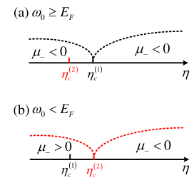
Figure 2: The comparison of the critical points $\eta_{c}^{(1)}$ and $\eta_{c}^{(2)}$ for (a) $\omega_{0}\geqslant E_{F}$ and (b) $\omega_{0}<E_{F}$. When $\omega_{0}\geqslant E_{F}$, $\eta_{c}^{(1)}>\eta_{c}^{(2)}$, and $\mu_{-}<0$ for both $0<\eta<\eta_{c}^{(1)}$ and $\eta>\eta_{c}^{(1)}$. When $\omega_{0}<E_{F}$, $\eta_{c}^{(1)}<\eta_{c}^{(2)}$, and $\mu_{-}<0$ for $\eta>\eta_{c}^{(2)}$ and $\mu_{-}>0$ for $0<\eta<\eta_{c}^{(2)}$.

In order to find the stable ground state, we should introduce the condition governed by $\partial^{2}\bar{E}_{\text{G}}/\partial\left(\left|\bar{\alpha}\right|\right)^{2}>0$. In terms of this stable condition, we find immediately that $\left|\bar{\alpha}\right|=0$ for $\eta<\eta_{c}^{(1)}$, where

$$\eta_{c}^{(1)}=\sqrt{\frac{\omega_{0}\left(\omega^{2}+\kappa^{2}\right)}{2\omega}},$$ (44)

and $\left|\bar{\alpha}\right|=\sqrt{\eta^{2}/\left(\omega^{2}+\kappa^{2}\right)-\omega_{0}^{2}\left(\omega^{2}+\kappa^{2}\right)/\left(4\omega^{2}\eta^{2}\right)}$ [i.e., Eq. (43)] for $\eta>\eta_{c}^{(1)}$. At the same time, we must notice the restrictive condition $\mu_{-}=\mu-\bar{\chi}<0$ in Eq. (37), which also induces a critical point

$$\eta_{c}^{(2)}=\sqrt{\frac{E_{F}\left(\omega^{2}+\kappa^{2}\right)}{2\omega}}.$$ (45)

When $\eta>\eta_{c}^{(2)}$, $\mu_{-}<0$.

From the critical points in Eqs. (44) and (45), we find that when $\omega_{0}\geqslant E_{F}$, $\eta_{c}^{(1)}>\eta_{c}^{(2)}$, and Eqs. (42)-(43) satisfy the condition $\mu_{-}<0$ for both $0<\eta<\eta_{c}^{(1)}$ and $\eta>\eta_{c}^{(1)}$ [see Fig. 2(a)]. However, when $\omega_{0}<E_{F}$, $\eta_{c}^{(1)}<\eta_{c}^{(2)}$, and only Eq. (43) satisfy the condition $\mu_{-}<0$ for $\eta>\eta_{c}^{(2)}$ [see Fig. 2(b)]. In other words, when $0<\eta<\eta_{c}^{(2)}$, $\mu_{-}\geqslant 0$, in which we should introduce a new scaled ground-state energy, as will be shown in the next subsection.

As a consequence, in the case of $\omega_{0}\geqslant E_{F}$, the scaled ground-state energy is written as

$$\bar{E}_{\text{G}}=\left\{\begin{array}[]{lcl}{-E_{F}}&&{0<\eta<\eta_{c}^{(1)}}\\ {-E_{F}+\frac{\omega\eta^{2}}{\omega^{2}+\kappa^{2}}-\frac{\omega_{0}^{2}\left(\omega^{2}+\kappa^{2}\right)}{4\omega\eta^{2}}}&&{\eta>\eta_{c}^{(1)}}\end{array}\right.,$$ (46)

and three parameters are given respectively by

$$\mu = \left\{\begin{array}[]{lcl}{2E_{F}-\omega_{0}}&&{0<\eta<\eta_{c}^{(1)}}\\ {2\left(E_{F}-\frac{\omega\eta^{2}}{\omega^{2}+\kappa^{2}}\right)}&&{\eta>\eta_{c}^{(1)}}\end{array}\right.,$$ (49)

$$\left|\bar{\alpha}\right| = \left\{\begin{array}[]{lcl}0&&{0<\eta<\eta_{c}^{(1)}}\\ \sqrt{\frac{\eta^{2}}{\omega^{2}+\kappa^{2}}-\frac{\omega_{0}^{2}\left(\omega^{2}+\kappa^{2}\right)}{4\omega^{2}\eta^{2}}}&&\eta>\eta_{c}^{(1)}\end{array}\right.,$$ (52)

$$\bar{m} = \left\{\begin{array}[]{lcl}1&&{0<\eta<\eta_{c}^{(1)}}\\ \frac{\omega_{0}\left(\omega^{2}+\kappa^{2}\right)}{2\omega\eta^{2}}&&{\eta>\eta_{c}^{(1)}}\end{array}\right..$$ (55)

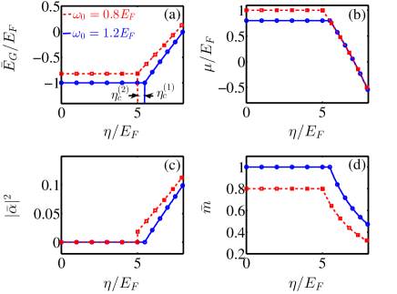
Figure 3: (a) The scaled ground-state energy $\bar{E}_{\text{G}}/E_{F}$, (b) the chemical potential $\mu/E_{F}$, (c) the scaled mean-photon number $\left|\bar{\alpha}\right|^{2}$, and (d) the scaled polarization $\bar{m}$ as functions of the effective atom-photon coupling strength $\eta/E_{F}$. The atom-number dependent cavity frequency and the cavity decay rate are given by $\omega=10E_{F}$ and $\kappa=20E_{F}$, respectively. When the effective resonant frequency is chosen as $\;\omega_{0}=1.2E_{F}$, $\eta_{c}^{(1)}=5.48E_{F}$. When $\;\omega_{0}=0.8E_{F}$, $\eta_{c}^{(2)}=$ $5E_{F}$. In these figures, the blue-solid and red-dashed lines represent the analytical results, while the open symbols correspond to numerical simulations.

The analytical results in Eqs. (46)-(55) show two typical properties. The first is that the first-order derivative of $\bar{E}_{\text{G}}$ with respect to ${\eta}$ is continuous but its second order is discontinuous, which means that a second-order phase transition from the N-I phase to the SR phase occurs at the critical point $\eta_{c}^{(1)}$. This property is similar to the case of ultracold Bose atoms YKW73 ; FTH73 . The other is that in the N-I phase no fermion-photon interaction occurs, whereas in the SR phase both the fermions and photons acquire the macroscopic collective excitations. Besides, $\bar{m}$ is inversely proportional to $\eta^{2}$ and $\mu$ is decreased with respect to $\eta^{2}$. In Figs. 3(a)-3(d), we plot $\bar{E}_{\text{G}}$, $\mu$, $\left|\bar{\alpha}\right|^{2}$, and $\bar{m}$ as functions of $\eta$. These figures show that our analytical results agree well with direct numerical simulations. Moreover, the above two typical properties are recovered naturally.

IV.2 $\mu_{-}\geqslant 0$

When

$$\mu_{-}=\mu-\bar{\chi}\geqslant 0,$$ (56)

$\Theta\left(\mu_{-}\right)=1$ and the scaled ground-state energy in Eq. (36) becomes

$$\bar{E}_{\text{G}}=-\frac{1}{4E_{F}}\left(\mu_{+}^{2}+\mu_{-}^{2}\right)+\omega\left|\bar{\alpha}\right|^{2}.$$ (57)

According to the discussions in the subsection A of this section and considering the stable condition governed by $\partial^{2}\bar{E}_{\text{G}}/\partial\left(\left|\bar{\alpha}\right|\right)^{2}>0$, we obtain

$$\mu=E_{F}\text{, \ \ \ \ }\left|\bar{\alpha}\right|=0\text{, \ \ \ \ }\bar{m}=\frac{\omega_{0}}{E_{F}},$$ (58)

for $0<\eta<\eta_{c}^{(2)}$. Since Eq. (58) should satisfy the condition $\mu_{-}\geqslant 0$ when $0<\eta<\eta_{c}^{(2)}$, we find that $\omega_{0}<E_{F}$ in this case. When $\eta>\eta_{c}^{(2)}$, $\mu_{-}<0$ [see Fig. 2(b)], in which we should combine with the previous discussions in the subsection A of this section.

As a consequence, in the case of $\omega_{0}<E_{F}$, the scaled ground-state energy is written as

$$\bar{E}_{\text{G}}=\left\{\begin{array}[]{lcl}{-\frac{E_{F}}{2}-\frac{\omega_{0}^{2}}{2E_{F}}}&&{0<\eta<\eta_{c}^{(2)}}\\ {-E_{F}+\frac{\omega\eta^{2}}{\omega^{2}+\kappa^{2}}-\frac{\omega_{0}^{2}\left(\omega^{2}+\kappa^{2}\right)}{4\omega\eta^{2}}}&&{\eta>\eta_{c}^{(2)}}\end{array}\right..$$ (59)

In addition, when $0<\eta<\eta_{c}^{\left(2\right)}$, $\mu$, $\left|\bar{\alpha}\right|$, and $\bar{m}$ are governed by Eq. (58), which means that the system is located at the N-II phase. When $\eta>\eta_{c}^{(2)}$, $\mu$, $\left|\bar{\alpha}\right|$, and $\bar{m}$ are governed by Eq. (43), which implies that the system is located at the SR phase. The scaled ground-state energy in Eq. (59) shows that the phase transition from the N-II phase to the SR phase is of the first order. Moreover, $\left|\bar{\alpha}\right|^{2}$ exhibits a sudden change at the critical point $\eta_{c}^{(2)}$, as shown by the red-dashed line in Fig. 3(c).

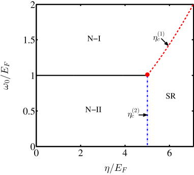
Figure 4: Phase diagram as a function of the effective resonant frequency $\omega_{0}/E_{F}$ and the effective fermion-photon coupling strength $\eta/E_{F}$. The atom-number dependent cavity frequency $\omega$ and the cavity decay rate $\kappa$ are the same as those in Fig. 3. When the effective resonant frequency is chosen as $\omega_{0}=E_{F}$, $\eta_{c}^{\left(1\right)}=\eta_{c}^{\left(2\right)}$.

Interestingly, when $\eta=\eta_{c}^{\left(2\right)}$, the scaled ground-state energies of the N-II and SR phases are equal, which means that these two phases coexist and the corresponding phase is called the N-II-SR mixed phase. In order to fully describe the fundamental properties of this mixed phase, we should introduce the fractions of the N-II and SR phases, $x_{0}$ and $1-x_{0}$. Moreover, we further obtain

$$\bar{E}_{\text{G}} = \mu-\frac{x_{0}\left(\omega_{0}^{2}+E_{F}^{2}\right)}{2E_{F}}$$ (60)

$$-\frac{\left(1-x_{0}\right)}{2}\left(E_{F}+\frac{\omega_{0}^{2}}{E_{F}}\right),$$

$$\mu = E_{F},$$ (61)

$$\left|\bar{\alpha}\right| = \sqrt{\frac{E_{F}^{2}-\omega_{0}^{2}}{2\omega E_{F}}},$$ (62)

$$\bar{m} = \frac{x_{0}\omega_{0}}{E_{F}}+\left(1-x_{0}\right)\frac{\omega_{0}\left(\omega^{2}+\kappa^{2}\right)}{2\omega\eta^{2}}.$$ (63)

The detailed derivation of Eqs. (60)-(63) is given by the Appendix A. Notice that since the atom densities are equal in both the N-II and SR phases, $x_{0}$ and $1-x_{0}$ are the arbitrary values ranging from $0$ to $1$. In addition, since $\bar{m}\neq 0$ in both the N-II and SR phases, the nonzero polarization in the N-II-SR mixed phase is caused by both the macroscopic collective excitation of the fermions and photons and the effective Zeeman field. We also find two first-order phase transitions from the N-II-SR phase to the N-II phase or the SR phase. These results are quite different from those in the N-I phase and the ultracold Bose atoms YKW73 ; FTH73 .

IV.3 Phase diagram

In Fig. 4, we plot the whole phase diagram, including the N-I phase, the N-II phase, the N-II-SR mixed phase, and the SR phase, for $\omega_{0}<E_{F}$ and $\omega_{0}\geqslant E_{F}$. As predicted previously, the phase transition from the N-I phase to the SR phase is of the second order, whereas the phase transition from the N-II phase to the SR phase is of the first order, due to the coexistence of the N-II and SR phases at the critical line. In addition, this phase diagram has a tricritical point (the red dot), at which the phase transition changes from the first order to the second order.

V Phase diagrams for $E_{b}\neq 0$ and $\eta\neq 0$

When both $\eta$ and $E_{b}$ exist, the properties of the Bogoliubov quasiparticle states are determined by both $\bar{\chi}$ and $\Delta$, as shown in the Hamiltonian (22). If $\bar{\chi}>\Delta$, the quasi-particle states are occupied for $\max\{0,\mu-\sqrt{\bar{\chi}^{2}-\Delta^{2}}\}<\epsilon_{\mathbf{k}}<\mu+\sqrt{\bar{\chi}^{2}-\Delta^{2}}$ ($\mu+\sqrt{\bar{\chi}^{2}-\Delta^{2}}>0$), and thus, the scaled ground-state energy is obtained by

$$\bar{E}_{\text{G}} = \bar{E}_{\text{G}}^{\text{SF}}+\omega\left|\bar{\alpha}\right|^{2}-\frac{1}{4E_{F}}\left[2\bar{\chi}\sqrt{\bar{\chi}^{2}-\Delta^{2}}-\Delta^{2}\ln\left(\frac{\bar{\chi}+\sqrt{\bar{\chi}^{2}-\Delta^{2}}}{\bar{\chi}-\sqrt{\bar{\chi}^{2}-\Delta^{2}}}\right)\right]\Theta\left(\bar{\mu}_{-}\right)\Theta\left(\bar{\chi}^{2}-\Delta^{2}\right)$$ (64)

$$-\frac{1}{4E_{F}}\left[\bar{\chi}\sqrt{\bar{\chi}^{2}-\Delta^{2}}+\mu\left(2\bar{\chi}-\sqrt{\mu^{2}+\Delta^{2}}\right)-\Delta^{2}\ln\left(-\frac{\bar{\chi}+\sqrt{\bar{\chi}^{2}-\Delta^{2}}}{\mu-\sqrt{\mu^{2}+\Delta^{2}}}\right)\right]\Theta\left(-\bar{\mu}_{-}\right)\Theta\left(\bar{\chi}^{2}-\Delta^{2}\right),$$

where $\bar{\mu}_{-}=\mu-\sqrt{\bar{\chi}^{2}-\Delta^{2}}$ and

$$\bar{E}_{\text{G}}^{\text{SF}} = \frac{\Delta^{2}}{4E_{F}}\ln\left(\frac{\sqrt{\mu^{2}+\Delta^{2}}-\mu}{E_{b}}\right)$$ (65)

$$-\frac{\mu}{4E_{F}}\left(\sqrt{\mu^{2}+\Delta^{2}}+\mu\right)-\frac{\Delta^{2}}{8E_{F}}$$

is the fully-paired ($\bar{m}=0$) SF energy. If $\bar{\chi}<\Delta$, $\bar{E}_{\text{G}}=\bar{E}_{\text{G}}^{\text{SF}}$. It can be seen clearly from Eq. (64) that the ground-state properties, including $\Delta$, $\mu$, and $\left|\bar{\alpha}\right|^{2}$, are governed by both $\eta$ and $E_{b}$. When $E_{b}=0$, $\bar{\mu}_{-}=\mu-\bar{\chi}$ and the corresponding scaled ground-state energy is the same as Eq. (36). When $\eta=0$, $\bar{\chi}=\omega_{0}$ and Eq. (64) reduces to Eq. (14) in Ref. JD09 and Eq. (8) in Ref. HC12 . When $E_{b}\neq 0$ and $\eta\neq 0$, a strong competition between the SF and SR properties occurs. Consequently, rich quantum phases can be predicted. Similarly, the Heaviside step function in Eq. (64) depends crucially on $\bar{\mu}_{-}$ and $\bar{\chi}^{2}-\Delta^{2}$, and thus, the following discussion of the ground-state properties should also be divided into four specific cases: $\bar{\mu}_{-}<0$ and $\bar{\chi}^{2}-\Delta^{2}\geqslant 0$, $\bar{\mu}_{-}<0$ and $\bar{\chi}^{2}-\Delta^{2}<0$, $\bar{\mu}_{-}\geqslant 0$ and $\bar{\chi}^{2}-\Delta^{2}\geqslant 0$, and $\bar{\mu}_{-}\geqslant 0$ and  $\bar{\chi}^{2}-\Delta^{2}<0$. Moreover, we will draw two conclusions for $\omega_{0}<E_{F}$ and $\omega_{0}\geqslant E_{F}$.

V.1 $\bar{\mu}_{-}<0$ and $\bar{\chi}^{2}-\Delta^{2}\geqslant 0$

When

$$\bar{\mu}_{-}=\mu-\sqrt{\bar{\chi}^{2}-\Delta^{2}}<0$$ (66)

and

$$\bar{\chi}^{2}-\Delta^{2}\geqslant 0,$$ (67)

$\Theta\left(\bar{\mu}_{-}\right)=0$ and $\Theta\left(\bar{\chi}^{2}-\Delta^{2}\right)=1$. Thus, the scaled ground-state energy in Eq. (64) becomes

$$\bar{E}_{\text{G}} = \bar{E}_{\text{G}}^{\text{SF}}+\omega\left|\bar{\alpha}\right|^{2}-\frac{1}{4E_{F}}\left[\bar{\chi}\sqrt{\bar{\chi}^{2}-\Delta^{2}}\right.$$ (68)

$$\left.-\Delta^{2}\ln\left(-\frac{\bar{\chi}+\sqrt{\bar{\chi}^{2}-\Delta^{2}}}{\mu-\sqrt{\mu^{2}+\Delta^{2}}}\right)\right.$$

$$\left.+\mu\left(2\bar{\chi}-\sqrt{\mu^{2}+\Delta^{2}}\right)\right].$$

From Eqs. (26)-(28) and (32), we obtain

$$\Delta\ln\left(\frac{\sqrt{\Delta^{2}+\mu^{2}}-\mu}{E_{b}}\right)+\Delta\ln\left[\frac{\left(\bar{\chi}+\sqrt{\bar{\chi}^{2}-\Delta^{2}}\right)\left(\sqrt{\Delta^{2}+\mu^{2}}+\mu\right)}{\Delta^{2}}\right] = 0,$$ (69)

$$\mu+\bar{\chi} = 2E_{F},$$ (70)

$$\left[-\frac{\omega^{2}\eta^{2}}{E_{F}\left(\omega^{2}+\kappa^{2}\right)}\frac{\mu+\sqrt{\bar{\chi}^{2}-\Delta^{2}}}{\bar{\chi}}+\omega\right]\left|\bar{\alpha}\right| = 0,$$ (71)

$$\frac{\left(\sqrt{\bar{\chi}^{2}-\Delta^{2}}+\mu\right)}{\bar{\chi}} = \frac{2E_{F}\bar{m}}{\omega_{0}}.$$ (72)

By further solving Eqs. (69)-(72), we obtain

$$\Delta=0\text{, \ \ }\mu=2E_{F}-\omega_{0}\text{, \ \ }\left|\bar{\alpha}\right|=0\text{, \ \ }\bar{m}=1,$$ (73)

or

$$\left\{\begin{array}[]{l}\Delta=0,\\ \mu=2\left(E_{F}-\frac{\omega\eta^{2}}{\omega^{2}+\kappa^{2}}\right),\\ \left|\bar{\alpha}\right|=\sqrt{\frac{\eta^{2}}{\omega^{2}+\kappa^{2}}-\frac{\omega_{0}^{2}\left(\omega^{2}+\kappa^{2}\right)}{4\omega^{2}\eta^{2}}},\\ \bar{m}=\frac{\omega_{0}\left(\omega^{2}+\kappa^{2}\right)}{2\omega\eta^{2}},\end{array}\right.$$ (74)

or

$$\left\{\begin{array}[]{l}\Delta=\sqrt{E_{b}\left(2\omega_{0}-E_{b}\right)},\\ \mu=2E_{F}-\omega_{0},\\ \left|\bar{\alpha}\right|=0,\\ \bar{m}=\frac{E_{b}-2\omega_{0}+2E_{F}}{2E_{F}},\end{array}\right.$$ (75)

or

$$\left\{\begin{array}[]{l}\Delta=\sqrt{E_{b}\left[\frac{2\omega\eta^{2}\left(2E_{F}+E_{b}\right)}{2\omega\eta^{2}+\left(\omega^{2}+\kappa^{2}\right)E_{F}}-E_{b}\right]},\\ \mu=2E_{F}-\frac{\omega\eta^{2}\left(2E_{F}+E_{b}\right)}{2\omega\eta^{2}+\left(\omega^{2}+\kappa^{2}\right)E_{F}},\\ \left|\bar{\alpha}\right|=\frac{\sqrt{\left(\omega^{2}+\kappa^{2}\right)}}{2}\sqrt{\left[\frac{\eta\left(2E_{F}+E_{b}\right)}{2\omega\eta^{2}+\left(\omega^{2}+\kappa^{2}\right)E_{F}}\right]^{2}-\frac{\omega_{0}^{2}}{\omega^{2}\eta^{2}}},\\ \bar{m}=\frac{\omega_{0}\left(\omega^{2}+\kappa^{2}\right)}{2\omega\eta^{2}}.\end{array}\right.$$ (76)

Since here the system has two dependent order parameters $\Delta$ and $\left|\bar{\alpha}\right|$, the ground-state stability should be determined by a $2\times 2$ Hessian matrix SB81 , which is defined as

$$M=\left[\begin{array}[]{cc}\frac{\partial^{2}\bar{E}_{\text{G}}}{\partial\Delta^{2}}&\frac{\partial^{2}\bar{E}_{\text{G}}}{\partial\Delta\partial\left|\bar{\alpha}\right|}\\ \frac{\partial^{2}\bar{E}_{\text{G}}}{\partial\left|\bar{\alpha}\right|\partial\Delta}&\frac{\partial^{2}\bar{E}_{\text{G}}}{\partial\left(\left|\bar{\alpha}\right|\right)^{2}}\end{array}\right].$$ (77)

If $M$ is positive definite (i.e., two eigenvalues of $M$ are positive), $\bar{E}_{\text{G}}$ has local minima and the system is located at the stable phase. If $M$ is indefinite (i.e., one eigenvalues is positive, while the other is negative), $\bar{E}_{\text{G}}$ has saddle points and the system is dynamically unstable. If $M$ is negative definite (i.e., two eigenvalues of $M$ are negative), $\bar{E}_{\text{G}}$ has a local maximum and the system is extremely unstable.

In terms of the stability condition given by the Hessian matrix (77), the ground states corresponding to the solutions (75) or (76) are unstable, whereas for the solutions (73) or (74) they become stable. Since $\Delta\equiv 0$ in both Eqs. (73) and (74), we can use the similar discussions in the subsection A of Sec. IV. For example, using the stable condition governed by $\partial^{2}\bar{E}_{\text{G}}/\partial\left(\left|\bar{\alpha}\right|\right)^{2}>0$, we obtain the superradiant critical point $\eta_{c}^{(1)}$, which separates the solutions (73) and (74). In addition, the restrictive conditions in Eqs. (66) and (67) lead to another critical point $\eta_{c}^{(2)}$. Comparing $\eta_{c}^{(1)}$ with $\eta_{c}^{(2)}$, we find that when $\omega_{0}\geqslant E_{F}$, i.e., $\eta_{c}^{(1)}>\eta_{c}^{(2)}$, $\bar{\mu}_{-}<0$ and $\bar{\chi}^{2}-\Delta^{2}\geqslant 0$, and thus, $\Delta$, $\mu$, $\left|\bar{\alpha}\right|$, and $\bar{m}$ are governed by Eq. (73) for $0<\eta<\eta_{c}^{(1)}$, and for $\eta>\eta_{c}^{(1)}$, they are governed by Eq. (74). When $\omega_{0}<E_{F}$, i.e., $\eta_{c}^{(1)}<\eta_{c}^{(2)}$, $\bar{\mu}_{-}\geqslant 0$ and $\bar{\chi}^{2}-\Delta^{2}\geqslant 0$, and thus, for $0<\eta<\eta_{c}^{(2)}$, the scaled ground-state energy changes and we will discuss the relevant results in the subsection D of this section. However, for $\eta>\eta_{c}^{(2)}$, $\bar{\mu}_{-}<0$ and $\bar{\chi}^{2}-\Delta^{2}\geqslant 0$, and thus,$\ \Delta$, $\mu$, $\left|\bar{\alpha}\right|$, and $\bar{m}$ are still governed by Eq. (74).

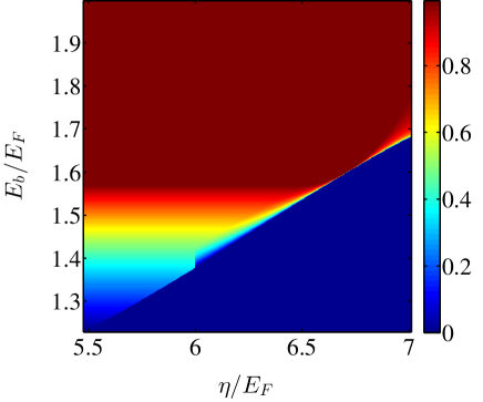
Figure 5: The fraction of the SF phase, $x_{2}$, as a function of the two-body binding energy $E_{b}/E_{F}$ and the effective fermion-photon coupling strength $\eta/E_{F}$, when the effective resonant frequency is chosen as $\omega_{0}=1.2E_{F}$. The atom-number dependent cavity frequency $\omega$ and the cavity decay rate $\kappa$ are the same as those in Fig. 3.

V.2 $\bar{\mu}_{-}<0$ and $\bar{\chi}^{2}-\Delta^{2}<0$

When

$$\bar{\mu}_{-}=\mu-\sqrt{\bar{\chi}^{2}-\Delta^{2}}<0$$ (78)

and

$$\bar{\chi}^{2}-\Delta^{2}<0,$$ (79)

$\Theta\left(\bar{\mu}_{-}\right)=0$ and $\Theta\left(\bar{\chi}^{2}-\Delta^{2}\right)=0$. Thus, the scaled ground-state energy in Eq. (64) becomes

$$\bar{E}_{\text{G}}=\bar{E}_{\text{G}}^{\text{SF}}+\omega\left|\bar{\alpha}\right|^{2}.$$ (80)

From Eqs. (26)-(28) and (32), we obtain

$$\Delta\ln\left(\frac{\sqrt{\Delta^{2}+\mu^{2}}-\mu}{E_{b}}\right) = 0,$$ (81)

$$\sqrt{\Delta^{2}+\mu^{2}}+\mu = 2E_{F},$$ (82)

$$2\omega\left|\bar{\alpha}\right| = 0,$$ (83)

$$\bar{m} = 0.$$ (84)

By further solving Eqs. (81)-(84), we obtain

$$\Delta=0\text{, \ \ \ \ }\mu=E_{F}\text{, \ \ \ }\left|\bar{\alpha}\right|=0\text{, \ \ \ \ }\bar{m}=0,$$ (85)

or

$$\Delta=\sqrt{2E_{F}E_{b}}\text{, \ }\mu=E_{F}-\frac{E_{b}}{2}\text{, }\left|\bar{\alpha}\right|=0\text{, \ }\bar{m}=0.$$ (86)

Since $\left|\bar{\alpha}\right|\equiv 0$ in Eqs. (85) and (86), we should introduce the stable condition governed by $\partial^{2}\bar{E}_{\text{G}}/\partial\Delta^{2}>0$ to find the stable ground state. According to this stable condition and the restrictive condition in Eqs. (78) and (79), we find that the ground state, with the solution (86), is stable for all $E_{b}$ and $\eta$.

V.3 The stable ground states for $\omega_{0}\geqslant E_{F}$

In terms of the above discussions in the subsections A and B of this section, we can obtain the stable ground-state properties for $\omega_{0}\geqslant E_{F}$. In this case, there exist two kinds of competition governed by the solutions (73), (74), and (86). When $0<\eta<\eta_{c}^{\left(1\right)}$, the solutions (73) and (86) dominates, whereas when $\eta>\eta_{c}^{\left(1\right)}$, the solutions (74) and (86) dominates. These solutions show two typical properties of the scaled ground-state energy. The first is that the scaled ground-state energy has a global minimum, i.e., the system is located at the N-I, SF, or SR phases. The other is that the scaled ground-state energy has two degenerate minima, which implies that two of these phases can coexist. Thus, for $\omega_{0}\geqslant E_{F}$, the results for the stable ground state are summarized as the following two situations: $0<\eta<\eta_{c}^{\left(1\right)}$ and $\eta>\eta_{c}^{\left(1\right)}$.

V.3.1 $0<\eta<\eta_{c}^{\left(1\right)}$

When $0<\eta<\eta_{c}^{\left(1\right)}$, it can be seen from Eqs. (73), (74), and (86) that the weak fermion-photon interaction has no effect on the systematic properties. In this case, only the N-I and SF phases can be found. More interestingly, when varying $E_{b}$, the ground-state energies for these two phases are equal, i.e., these two phases coexist and the corresponding phase is called the N-I-SF mixed phase.

From the phase equilibrium condition DES07 ; LH08 , we find that for $E_{b}\!<\!2\left[\omega_{0}-\left(\sqrt{2}-1\right)E_{F}\right]$, $\Delta=0$, and $\bar{E}_{\text{G}}$, $\mu$, and $\bar{m}$ are governed by Eqs. (31) and (33). This implies that the system is located at the N-I phase. For $2\left[\omega_{0}-\left(\sqrt{2}-1\right)E_{F}\right]<E_{b}<2\!\left[\omega_{0}-\left(2-\sqrt{2}\right)E_{F}\right]$, we find $\bar{E}_{\text{G}}\left(\mu\text{, }\Delta\neq 0\right)=\bar{E}_{\text{G}}\left(\mu\text{, }\Delta=0\right)$, which implies that the system is located at the N-I-SF mixed phase. In order to fully describe the fundamental properties of this mixed phase, we should introduce the fractions of the N-I and SF phases, $x_{1}$ and $1-x_{1}$. Moreover, we further obtain

$$\bar{E}_{\text{G}} = \mu-\frac{x_{1}}{4E_{F}}\left(\frac{2\omega_{0}-E_{b}}{2-\sqrt{2}}\right)^{2}$$ (87)

$$-\frac{1-x_{1}}{4E_{F}}\left(\frac{2\omega_{0}-E_{b}}{2-\sqrt{2}}\right)^{2},$$

$$\Delta = \sqrt{\frac{2\omega_{0}E_{b}-E_{b}^{2}}{\sqrt{2}-1}},$$ (88)

$$\mu = \frac{\sqrt{2}\omega_{0}-E_{b}}{2-\sqrt{2}},$$ (89)

$$\bar{m} = 1-x_{1},$$ (90)

where $x_{1}=2\sqrt{2}E_{F}/\left(2\omega_{0}-E_{b}\right)-\sqrt{2}-1$. The detailed derivation of the above results is given by the Appendix B. For $E_{b}>2\!\left[\omega_{0}-\left(2-\sqrt{2}\right)E_{F}\right]$, we find

$$\bar{E}_{\text{G}}=-\frac{E_{F}}{2}\text{, \ }\Delta=\sqrt{2E_{F}E_{b}}\text{, }\mu=E_{F}-\frac{E_{b}}{2}\text{, }\bar{m}=0,$$ (91)

which indicates that the system is located at the SF phase. The analytical results in Eqs. (31), (33), and (87)-(91) are the same as those in Refs. LH08 ; DE15 , as expected. They show that when increasing $E_{b}$, two first-order phase transitions from the N-I phase to the N-I-SF mixed phase or from the N-I-SF mixed phase to the SF phase emerge DES06 ; HC12 ; LH08 ; DE15 ; KBG06 ; PFB03 ; GBP06 ; MWZ06 . Moreover, the ratio of the scaled polarization to the dimensionless mean-field gap in the N-II-SF mixed phase, $\bar{m}/\left(\Delta/E_{F}\right)$, is decreased.

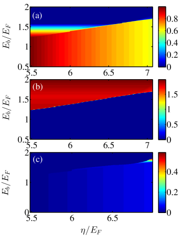
Figure 6: (a) The scaled polarization $\bar{m}$, (b) the mean-field gap $\Delta/E_{F}$, and (c) the scaled mean-photon number $\left|\bar{\alpha}\right|^{2}$ as functions of the two-body binding energy $E_{b}/E_{F}$ and the effective fermion-photon coupling strength $\eta/E_{F}$, when the effective resonant frequency is chosen as $\omega_{0}=1.2E_{F}$. The atom-number dependent cavity frequency $\omega$ and the cavity decay rate $\kappa$ are the same as those in Fig. 3.

V.3.2 $\eta>\eta_{c}^{\left(1\right)}$

When $\eta>\eta_{c}^{\left(1\right)}$, it can be seen from Eq. (74) that a non-zero $\left|\bar{\alpha}\right|$ emerges, which means that the fermion-photon interaction has a significant effect on the systematic properties. In this case, only the SF and SR phases can be found. More interestingly, when varying $E_{b}$ and $\eta$, the ground-state energies for these two phases are equal, i.e., these two phases coexist and the corresponding phase is called the SF-SR mixed phase.

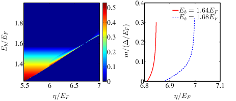
Figure 7: (a) The ratio of the scaled polarization to the dimensionless mean-field gap in the N-II-SF mixed state, $\bar{m}/\left(\Delta/E_{F}\right)$, as a function of the two-body binding energy $E_{b}/E_{F}$ and the effective fermion-photon coupling strength $\eta/E_{F}$, when the effective resonant frequency is chosen as $\omega_{0}=1.2E_{F}$. The atom-number dependent cavity frequency $\omega$ and the cavity decay rate $\kappa$ are the same as those in Fig. 3. (b) For a fixed $E_{b}=E_{F}$ (the red-solid line) and $E_{b}=1.1E_{F}$ (the blue-dashed line), $\bar{m}/\left(\Delta/E_{F}\right)$ varies as a function of $\eta/E_{F}$.

From the phase equilibrium condition DES07 ; LH08 , we find four stable regions as follows.

(i) When $E_{b}<E_{b}^{\left(1\right)}$, $\Delta=0$, and $\bar{E}_{\text{G}}$, $\mu$, $\left|\bar{\alpha}\right|$, and $\bar{m}$ are governed by Eqs. (46)-(55). These mean that the system is located at the SR phase.

(ii) When $E_{b}^{\left(1\right)}\Theta\left(\eta_{c}^{\left(3\right)}-\eta\right)\!<\!E_{b}\!<\!2\left[\omega_{0}-\left(2-\sqrt{2}\right)E_{F}\right]\Theta\left(\eta_{c}^{\left(3\right)}-\eta\right)$ or $E_{b}^{\left(2\right)}\Theta\left(\eta-\eta_{c}^{\left(3\right)}\right)\!<\!E_{b}\!<\!2\left[\omega_{0}-\left(2-\sqrt{2}\right)E_{F}\right]\Theta\left(\eta-\eta_{c}^{\left(3\right)}\right)$, with $\eta_{c}^{\left(3\right)}=\omega_{0}\sqrt{\left(\omega^{2}+\kappa^{2}\right)/2\omega}$, we find $\bar{E}_{\text{G}}\left(\mu\text{, }\Delta\neq 0\text{, }\left|\bar{\alpha}\right|=0\right)=\bar{E}_{\text{G}}\left(\mu\text{, }\Delta=0\text{, }\left|\bar{\alpha}\right|=0\right)$, which means that the N-I and SF phases coexist and the corresponding phase is called the N-I-SF mixed phase. We further obtain $\bar{E}_{\text{G}}$, $\Delta$, $\mu$, and $\bar{m}$, which are governed by Eqs. (87)-(90).

(iii) When $E_{b}^{\left(1\right)}\!<\!E_{b}\!<\!E_{b}^{\left(2\right)}\Theta\left(\eta-\eta_{c}^{\left(3\right)}\right)$, we find $\bar{E}_{\text{G}}\left(\mu\text{, }\Delta\neq 0\text{, }\left|\bar{\alpha}\right|=0\right)=\bar{E}_{\text{G}}\left(\mu\text{, }\Delta=0\text{, }\left|\bar{\alpha}\right|\neq 0\right)$, which implies that the system is located at the SF-SR mixed phase. In order to fully describe the fundamental properties of this mixed phase, we should introduce the fractions of the SF and SR phases, $x_{2}$ and $1-x_{2}$. Moreover, we further obtain

$$\bar{E}_{\text{G}} = \mu-x_{2}\frac{1}{2E_{F}}\left(\mu+\frac{E_{b}}{2}\right)^{2}$$ (92)

$$-\left(1-x_{2}\right)\left[\frac{\mu^{2}}{4E_{F}A}+\frac{\omega_{0}^{2}\left(\omega^{2}+\kappa^{2}\right)}{4\omega\eta^{2}}\right],$$

$$\Delta = \sqrt{E_{b}\left(E_{b}+2\mu\right)},$$ (93)

$$\mu = \frac{-E_{b}A\pm\sqrt{A^{2}E_{b}^{2}-2A\left(2A-1\right)B}}{2A-1},$$ (94)

$$\left|\bar{\alpha}\right| = \frac{1}{2}\sqrt{\frac{\mu^{2}\eta^{2}}{\left(\omega^{2}+\kappa^{2}\right)E_{F}^{2}A^{2}}-\frac{\omega_{0}^{2}\left(\omega^{2}+\kappa^{2}\right)}{\omega^{2}\eta^{2}}},$$ (95)

$$\bar{m} = \left(1-x_{2}\right)\frac{\omega_{0}\left(\omega^{2}+\kappa^{2}\right)}{2\omega\eta^{2}},$$ (96)

where $A=1-\omega\eta^{2}/\left[E_{F}\left(\omega^{2}+\kappa^{2}\right)\right]$, $B=E_{b}^{2}/4-E_{F}\omega_{0}^{2}\left(\omega^{2}+\kappa^{2}\right)/\left(2\omega\eta^{2}\right)$, and $x_{2}=\left(2E_{F}A-\mu\right)/\left(2\mu A-\mu+E_{b}A\right)$. The detailed derivation of the above results is displayed in the Appendix C. In principle, $E_{b}^{\left(1\right)}$ and $E_{b}^{\left(2\right)}$ can be obtained analytically. However, their expressions are so complicated that here we donot list them.

The analytical results in Eqs. (93)-(96) show that the predicted SF-SR mixed phase has the following typical properties:

$\bullet$ When $x_{2}=0$, the system is located at the SR phase with $\bar{m}=$ $\omega_{0}\left(\omega^{2}+\kappa^{2}\right)/\left(2\omega\eta^{2}\right)$, whereas when $x_{2}=1$, the system enters into the SF phase with $\bar{m}=0$. The above explicit expressions show that the nonzero $\bar{m}$ in the SF-SR mixed phase is only caused by the macroscopic collective excitation of both the fermions and photons, which is different from that of the N-I-SF phase.

$\bullet$ For a relative small $E_{b}$ or larger $\eta$, $x_{2}\rightarrow 0$, as shown in Fig. 5. This means that the systematic properties are mainly governed by the SR properties. Whenever increasing $\eta$ or $E_{b}$, $\bar{m}$ is decreased, and $\Delta$ and $\left|\bar{\alpha}\right|$ are increased, as shown in Figs. 6(a)-6(c).

$\bullet$ For a relative small $\eta$ or larger $E_{b}$, $x_{2}\rightarrow 1$, as also shown in Fig. 5. This means that the systematic properties are mainly governed by the SF properties. In this case, $\bar{m}$ approaches zero, as also shown in Fig. 6(a), and $\Delta$ and $\left|\bar{\alpha}\right|$ almost reach their maximum values, as also shown in Figs. 6(b) and 6(c).

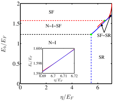
Figure 8: Phase diagram as a function of the two-body binding energy $E_{b}/E_{F}$ and the effective atom-photon coupling strength $\eta/E_{F}$, when the effective resonant frequency is chosen as $\omega_{0}=1.2E_{F}$. The atom-number dependent cavity frequency $\omega$ and the cavity decay rate $\kappa$ are also the same as in Fig. 3. Inset: the region of the phase boundaries approaching each other.

$\bullet$ For the intermediate $\eta$ and $E_{b}$, both $x_{2}$ and $1-x_{2}$ are the finite values ranging from $0$ to $1$, as also shown in Fig. 5. These mean that the SF and SR properties have a strong competition. When increasing $E_{b}$, $\bar{m}$ is decreased, and thus, both $\Delta$ and $\left|\bar{\alpha}\right|$ are increased, as also shown in Figs. 6(a)-6(c). However, when increasing $\eta$, $\bar{m}$ is increased, due to the rapid increasing of $1-x_{2}$, i.e., the fraction of the SR phase, and thus, both $\Delta$ and $\left|\bar{\alpha}\right|$ are decreased, as also shown in Figs. 6(a)-6(c). This is quite different from that in the SR phase, in which when increasing $\eta$, $\bar{m}$ is decreased [see Fig. 3(d)]. In order to see clearly the evolution of $\bar{m}$ and $\Delta$, we plot $\bar{m}/\left(\Delta/E_{F}\right)$ as a function of $\eta$ and $E_{b}$ in Fig. 7. For a fixed $E_{b}$, when increasing $\eta$, $\bar{m}/\left(\Delta/E_{F}\right)$ is increased, as shown in Figs. 7(a) and 7(b). Based on this conclusion, we expect that in real experiments we can tune $\eta$ and $E_{b}$ to find a relative large regime that the magnetic and SF properties coexist. This is also different from the situation in the N-II-SF mixed phase, in which when increasing $E_{b}$ the coexisted regime becomes smaller and smaller. In addition, $\bar{m}/\left|\bar{\alpha}\right|$ has a similar behavior, and thus, is not addressed here.

(iv) When $E_{b}\!>\!2\!\left[\omega_{0}-\left(2-\sqrt{2}\right)E_{F}\right]\Theta\left(\eta_{c}^{\left(3\right)}-\eta\right)$ or $E_{b}>E_{b}^{\left(2\right)}\Theta\left(\eta-\eta_{c}^{\left(3\right)}\right)$, $\left|\bar{\alpha}\right|=0$, and $\bar{E}_{\text{G}}$, $\Delta$, $\mu$, and $\bar{m}$ are governed by Eq. (91). These mean that the system is located at the SF phase.

V.3.3 Phase diagram

In Fig. 8, we plot the whole phase diagram, including the N-I phase, the N-I-SR mixed phase, the SF-SR mixed phase, the SF phase, and the SR phase, for $0<\eta<\eta_{c}^{\left(1\right)}$ and $\eta>\eta_{c}^{\left(1\right)}$. The phase transitions, from the N-I-SF mixed phase to the N-I phase or the SF phase or the SR phase or the SF-SR mixed phase and from the SF-SR mixed phase to the SF phase or the SP phase, are of the first order, due to the existence of the N-I-SF and SF-SR mixed phases. However, the phase transition from the N-I phase to the SR phase is of the second order. In addition, this phase diagram has a tricritical point (the green dot), at which the phase transition changes from the first order to the second order.

V.4 $\bar{\mu}_{-}\geqslant 0$ and $\bar{\chi}^{2}-\Delta^{2}\geqslant 0$

When

$$\bar{\mu}_{-}=\mu-\sqrt{\bar{\chi}^{2}-\Delta^{2}}\geqslant 0$$ (97)

and

$$\bar{\chi}^{2}-\Delta^{2}\geqslant 0,$$ (98)

$\Theta\left(\bar{\mu}_{-}\right)=1$ and $\Theta\left(\bar{\chi}^{2}-\Delta^{2}\right)=1$. Thus, the scaled ground-state energy in Eq. (64) becomes

$$\bar{E}_{\text{G}} = \bar{E}_{\text{G}}^{\text{SF}}+\omega\left|\bar{\alpha}\right|^{2}-\frac{1}{4E_{F}}\left[2\bar{\chi}\sqrt{\bar{\chi}^{2}-\Delta^{2}}\right.$$ (99)

$$\left.-\Delta^{2}\ln\left(\frac{\bar{\chi}+\sqrt{\bar{\chi}^{2}-\Delta^{2}}}{\bar{\chi}-\sqrt{\bar{\chi}^{2}-\Delta^{2}}}\right)\right].$$

From Eqs. (26)-(28) and (32), we obtain

$$\Delta\ln\left(\frac{\sqrt{\Delta^{2}+\mu^{2}}-\mu}{E_{b}}\right)+\Delta\ln\left[\frac{2\bar{\chi}\left(\bar{\chi}+\sqrt{\bar{\chi}^{2}-\Delta^{2}}\right)-\Delta^{2}}{\Delta^{2}}\right] = 0,$$ (100)

$$\sqrt{\Delta^{2}+\mu^{2}}+\mu = 2E_{F},$$ (101)

$$\left[-\frac{2\omega^{2}\eta^{2}}{E_{F}\left(\omega^{2}+\kappa^{2}\right)}\frac{\sqrt{\bar{\chi}^{2}-\Delta^{2}}}{\bar{\chi}}+\omega\right]\left|\bar{\alpha}\right| = 0,$$ (102)

$$\frac{2\sqrt{\bar{\chi}^{2}-\Delta^{2}}}{\bar{\chi}} = \frac{2E_{F}\bar{m}}{\omega_{0}}.$$ (103)

By further solving Eqs. (100)-(103), we obtain the following solutions:

$$\Delta=0\text{, \ }\mu=E_{F}\text{, \ \ }\left|\bar{\alpha}\right|=0\text{, \ }\bar{m}=\frac{\omega_{0}}{E_{F}},$$ (104)

or

$$\left\{\begin{array}[]{l}\Delta=\sqrt{\sqrt{2E_{F}E_{b}}\left(2\omega_{0}-\sqrt{2E_{F}E_{b}}\right)},\text{ }\\ \mu=E_{F}+\frac{E_{b}}{2}-\frac{\omega_{0}\sqrt{2E_{F}E_{b}}}{2E_{F}},\text{ }\\ \left|\bar{\alpha}\right|=0,\\ \bar{m}=\frac{\sqrt{\omega_{0}^{2}-\sqrt{2E_{F}E_{b}}\left(2\omega_{0}-\sqrt{2E_{F}E_{b}}\right)}}{E_{F}},\end{array}\right.$$ (105)

or

$$\left\{\begin{array}[]{l}\Delta=\sqrt{2E_{F}E_{b}}\sqrt{\frac{2\omega\eta^{2}-E_{F}\left(\omega^{2}+\kappa^{2}\right)}{2\omega\eta^{2}+E_{F}\left(\omega^{2}+\kappa^{2}\right)}},\\ \mu=E_{F}+\frac{E_{b}}{2}-\frac{2\omega\eta^{2}E_{b}}{2\omega\eta^{2}+E_{F}\left(\omega^{2}+\kappa^{2}\right)},\\ \left|\bar{\alpha}\right|=\sqrt{\frac{2\eta^{2}E_{F}E_{b}\left(\omega^{2}+\kappa^{2}\right)}{\left[2\omega\eta^{2}+E_{F}\left(\omega^{2}+\kappa^{2}\right)\right]^{2}}-\frac{\omega_{0}^{2}\left(\omega^{2}+\kappa^{2}\right)}{4\omega^{2}\eta^{2}}},\\ \bar{m}=\frac{\omega_{0}\left(\omega^{2}+\kappa^{2}\right)}{2\omega\eta^{2}}.\end{array}\right.$$ (106)

In terms of the stability condition given by the Hessian matrix (77), the ground states corresponding to the solutions (105) and (106) are unstable, whereas for the solution (104) it becomes stable. Since $\Delta\equiv 0$ in Eq. (104), we can use the similar discussions in the subsection B of Sec. IV. For instance, using the stable condition governed by $\partial^{2}\bar{E}_{\text{G}}/\partial\left(\left|\bar{\alpha}\right|\right)^{2}>0$ and the restrictive conditions in Eqs. (97) and (98), we find that when $\omega_{0}<E_{F}$, $\bar{\mu}_{-}\geqslant 0$ and $\bar{\chi}^{2}-\Delta^{2}\geqslant 0$, and thus, for $0<\eta<\eta_{c}^{(2)}$, $\Delta$, $\mu$, $\left|\bar{\alpha}\right|$, and $\bar{m}$ are governed by Eq. (104), whereas for $\eta>\eta_{c}^{(2)}$, $\bar{\mu}_{-}<0$ and $\bar{\chi}^{2}-\Delta^{2}\geqslant 0$, we should combine with the previous discussions in the subsection A of this section, and thus, $\Delta$, $\mu$, $\left|\bar{\alpha}\right|$, and $\bar{m}$ are governed by Eq. (74).

V.5 $\bar{\mu}_{-}\geqslant 0$ and $\bar{\chi}^{2}-\Delta^{2}<0$

When

$$\bar{\mu}_{-}=\mu-\sqrt{\bar{\chi}^{2}-\Delta^{2}}\geqslant 0$$ (107)

and

$$\bar{\chi}^{2}-\Delta^{2}<0,$$ (108)

$\Theta\left(\bar{\mu}_{-}\right)=1$ and $\Theta\left(\bar{\chi}^{2}-\Delta^{2}\right)=0$. The scaled ground-state energy in Eq. (64) becomes

$$\bar{E}_{\text{G}}=\bar{E}_{\text{G}}^{\text{SF}}+\omega\left|\bar{\alpha}\right|^{2},$$ (109)

which is the same as Eq. (80). Thus, the stable ground-state properties are the same with those in the subsection B of this section.

V.6 The stable ground states for $\omega_{0}<E_{F}$

In terms of the above discussions in the subsections A, D, and E of this section, we can obtain the stable ground-state properties for $\omega_{0}<E_{F}$. In this case, there also exist two kinds of competition governed by the solutions (74), (86), and (104). When $0<\eta<\eta_{c}^{\left(2\right)}$, the solutions (86) and (104) dominates, whereas when $\eta>\eta_{c}^{\left(2\right)}$, the solutions (74) and (86) dominates. These solutions also show two typical properties of the scaled ground-state energy. The first is that the scaled ground-state energy has a global minimum, i.e., the system is located at the N-II, SF, and SR phases. The other is that the scaled ground-state energy has two degenerate minima, which implies that two of these phases can coexist. Thus, for $\omega_{0}<E_{F}$, the results for the stable ground state are summarized as the following two situations: $0<\eta<\eta_{c}^{\left(2\right)}$ and $\eta>\eta_{c}^{\left(2\right)}$.

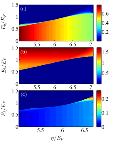
Figure 9: (a) The scaled polarization $\bar{m}$, (b) the mean-field gap $\Delta/E_{F}$, and (c) the scaled mean-photon number $\left|\bar{\alpha}\right|^{2}$ as functions of the two-body binding energy $E_{b}/E_{F}$ and the effective fermion-photon coupling strength $\eta/E_{F}$, when the effective resonant frequency is chosen as $\omega_{0}=0.8E_{F}$. The atom-number dependent cavity frequency $\omega$ and the cavity decay rate $\kappa$ are the same as those in Fig. 3.

V.6.1 $0<\eta<\eta_{c}^{\left(2\right)}$

When $0<\eta<\eta_{c}^{\left(2\right)}$, it can be seen from Eqs. (74), (86), and (104) that the weak fermion-photon interaction has no effect on the systematic properties. In this case, only the N-II and SF phases can be found. More interestingly, when varying $E_{b}$, the ground-state energies for these two phases are equal, i.e., these two phases coexist and the corresponding phase is called the N-II-SF mixed phase.

From the phase equilibrium condition DES07 ; LH08 , we find that for $E_{b}<2\left(\sqrt{E_{F}^{2}+\omega_{0}^{2}}-E_{F}\right)$, $\Delta=0$, and $\bar{E}_{\text{G}}$, $\mu$, and $\bar{m}$ are governed by Eqs. (34) and (35). This implies that the system is located at the N-II phase. For $2\!\left(\!\sqrt{E_{F}^{2}+\omega_{0}^{2}}-E_{F}\right)\!<\!E_{b}\!<\!2\left(\!E_{F}-\sqrt{E_{F}^{2}-\omega_{0}^{2}}\right)\Theta\left(\omega_{0}-\omega_{01}\right)$, where $\omega_{01}=E_{b}\left(1+\sqrt{2}\right)/2$ is determined by $\mu_{c1}=\omega_{0}$, we find $\bar{E}_{\text{G}}\left(\mu\text{, }\Delta=0\right)=\bar{E}_{\text{G}}\left(\mu\text{, }\Delta\neq 0\right)$. This implies that the system is located at the N-II-SF mixed phase. In order to fully describe the fundamental properties of this mixed phase, we should introduce the fractions of the N-II and SF phases, $x_{3}$ and $1-x_{3}$. Moreover, we further obtain

$$\bar{E}_{\text{G}} = \mu-\frac{x_{3}}{2E_{F}}\left(\frac{\omega_{0}^{2}}{E_{b}}+\frac{E_{b}}{4}\right)^{2}$$ (110)

$$-\left(1-x_{3}\right)\frac{\left(4\omega_{0}^{2}+E_{b}^{2}\right)^{2}}{32E_{F}E_{b}^{2}},$$

$$\Delta = \sqrt{\frac{E_{b}^{2}+4\omega_{0}^{2}}{2}},$$ (111)

$$\mu = \frac{\omega_{0}^{2}}{E_{b}}-\frac{E_{b}}{4},$$ (112)

$$\bar{m} = \left(1-x_{3}\right)\frac{\omega_{0}}{E_{F}},$$ (113)

where $x_{3}=1/2+2E_{F}/E_{b}-2\omega_{0}^{2}/E_{b}^{2}$. The detailed derivation of the above results is given by the Appendix B. For $E_{b}>2\left(E_{F}-\sqrt{E_{F}^{2}-\omega_{0}^{2}}\right)\Theta\left(\omega_{01}-\omega_{0}\right)$, we find that $\bar{E}_{\text{G}}$, $\Delta$, $\mu$, and $\bar{m}$ are governed by Eq. (91), which also indicates that the system is located at the SF phase. The analytical results in Eqs. (34), (35), (91), and (110)-(113) are also the same as those in Refs. LH08 ; DE15 , as expected. The basic properties of the N-II-SF mixed phase are similar to those in the N-I-SF mixed phase, and thus, are not discussed here.

V.6.2 $\eta>\eta_{c}^{\left(2\right)}$

When $\eta>\eta_{c}^{\left(2\right)}$, it can be seen from Eq. (74) that the fermion-photon interaction plays a significant role in the systematic properties, which are sharply contrast to the case of $0<\eta<\eta_{c}^{\left(2\right)}$ and similar to the case of $\eta>\eta_{c}^{\left(1\right)}$ in the subsubsection 2 of this section. In terms of Eqs. (74) and (86), we plot $\Delta$, $\mu$, $\left|\bar{\alpha}\right|$, and $\bar{m}$ as functions of $E_{b}$ and $\eta$ in Fig. 9, and find three stable regions as follows.

(i) When $E_{b}<E_{b}^{\left(1\right)}$, $\Delta=0$, and $\bar{E}_{\text{G}}$, $\mu$, $\left|\bar{\alpha}\right|$, and $\bar{m}$ are governed by Eqs. (59) and (43). These mean that the system is located at the SR phase.

(ii) When $E_{b}^{\left(1\right)}\!<\!E_{b}\!<\!E_{b}^{\left(2\right)}$, we find $\bar{E}_{\text{G}}\left(\mu\text{, }\Delta\neq 0\text{, }\left|\bar{\alpha}\right|=0\right)=\bar{E}_{\text{G}}\left(\mu\text{, }\Delta=0\text{, }\left|\bar{\alpha}\right|\neq 0\right)$, which means that the SF and SR phases coexist and the corresponding phase is called the SF-SR mixed phase. We further obtain $\bar{E}_{\text{G}}$, $\Delta$, $\mu$, $\left|\bar{\alpha}\right|$, and $\bar{m}$, which are governed by Eqs. (92)-(96). The other typical properties in this SF-SR mixed phase are the same as those in the region of $\eta\geqslant\eta_{c}^{\left(1\right)}$, and thus, are not addressed here.

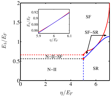
Figure 10: Phase diagram as a function of the two-body binding energy $E_{b}/E_{F}$ and the effective atom-photon coupling strength $\eta/E_{F}$, when the effective resonant frequency is chosen as $\omega_{0}=0.8E_{F}$. The atom-number dependent cavity frequency $\omega$ and the cavity decay rate $\kappa$ are also same as those in Fig. 3. Inset: the region of the phase boundaries approaching each other.

(iii) When $E_{b}>E_{b}^{\left(2\right)}$, $\left|\bar{\alpha}\right|=0$, and $\bar{E}_{\text{G}}$, $\Delta$, $\mu$, and $\bar{m}$ are governed by Eq. (91). These mean that the system is located at the SF phase.

V.6.3 Phase diagram

In Fig. 10, we plot the whole phase diagram, including the N-II phase, the N-II-SR mixed phase, the SF-SR mixed phase, the SF phase, and the SR phase, for $0<\eta<\eta_{c}^{\left(2\right)}$ and $\eta>\eta_{c}^{\left(2\right)}$. All the phase transitions are of the first order, due to the existence of the N-II-SR and SF-SR mixed phases.

VI Parameter estimation and possible experimental observation

We now take ⁴⁰K atom as an example to estimate the related parameters. For the fermionic ⁴⁰K atoms with the Fermi energy $E_{F}\sim 0.73$ MHz, the ground states with ²S_1/2 are given by $\left|\uparrow\right\rangle=\left|F=9/2,m_{F}=9/2\right\rangle$ and $\left|\downarrow\right\rangle=\left|F=9/2,m_{F}=7/2\right\rangle$, and the excited states with ²P_1/2 are chosen as $\left|1\right\rangle=\left|F=9/2,m_{F}=7/2\right\rangle$ and $\left|2\right\rangle=\left|F=9/2,m_{F}=9/2\right\rangle$, where $F$ and $m_{F}$ denote the total angular momentum and magnetic quantum numbers, respectively.

Due to the optical properties of the ⁴⁰K D1-line, the cavity length and the wavelengths of the transverse pumping lasers are chosen as $178$ $\mu$m and $770$ nm, respectively. In this case, both the fermion-photon coupling strengths $g_{1}$ and $g_{2}$ have the order of MHz, which is responsible for the rotating-wave approximation for deriving the Hamiltonians (4) and (5). When the waist radius of the cavity mode is given by $27$ $\mu$m and the cavity has a finesse with the order of $10^{5}$, the cavity decay rate $\kappa$ has the order of MHz. Since the effective fermion-photon coupling strength $\eta=\sqrt{N}g_{1}\Omega_{1}^{\ast}/\left(2\Delta_{1}\right)$ $=\sqrt{N}g_{2}\Omega_{2}^{\ast}/\left(2\Delta_{2}\right)$ is enhanced by a factor $\sqrt{N}$, it can reach the order of MHz by varying the Rabi frequencies of the transverse pumping lasers, even if the large detunings for ensuring the adiabatical approximation in deriving the Hamiltonians (9) is taken into account. The effective resonant frequency $\omega_{0}=$ $\left(\tilde{\omega}_{\downarrow}-\tilde{\omega}_{\uparrow}\right)/2$ and the atom-number dependent cavity frequency $\omega=N\zeta+\tilde{\omega}$ are controlled easily by varying the frequencies of the driving and transverse pumping lasers. In experiments KB10 , $\omega_{0}$ and $\omega$ can be tuned from $-$GHz to GHz, and even goes beyond this regime.

In addition, the 2D degenerate Fermi gas has been realized experimentally by a 1D deep optical lattice along the third dimension, where the tunneling between different layers is suppressed completely KM10 ; BF11 ; MF11 ; MK12 ; MGR15 . The 1D optical lattice potential $V_{0}\sin^{2}(2\pi x/\lambda_{w})$ can be generated using two counter-propagating laser beams (parallel to the $x$ axis with wavelength $\lambda_{w}$). In such a case, $E_{b}\simeq 0.915\hbar\omega_{L}\exp(\sqrt{2\pi}l_{L}/a_{s})/\pi$, where $\omega_{L}=\sqrt{8\pi^{2}V_{0}/(m\lambda_{w}^{2})}$ is the effective trapping frequency along the $x$ axis, $l_{L}=\sqrt{\hbar/(m\omega_{L})}$, and $a_{s}$ is the 3D s-wave scattering length JL15 . Therefore, $E_{b}$ can be tuned by varying the 3D s-wave scattering length $a_{s}$ via the Feshbash resonance and reach the order of MHz CC10 . Based on the above estimation, all parameters used to plot Figs. 3-10 could be realized in experiments.

Finally, we address briefly how to detect the predicted quantum phases and phase diagrams, which are mainly governed by the mean-field gap $\Delta$, the scaled mean-photon number $\left|\bar{\alpha}\right|^{2}$, and the scaled polarization $\bar{m}$. In experiments, the mean-field gap can be measured by the radio-frequency excitation spectra, i.e., the fractional loss of the fermions in one of the lowest substates through varying the radio-frequency frequency CC04 , the polarization and the properties of the mixed phase can be measured by observing the different density distributions between the two-component Fermi gas GBP06 ; MWZ06 , and the mean-photon number can be detected using calibrated single-photon counting modules, which allow us to monitor the intracavity light intensity in situ KB10 . Based on these developed experimental techniques, we believe that our predicted quantum phases and phase diagrams could be detected in future experiments.

VII Discussion and Conclusion

Before ending up this paper, we make one remark. In real experiments, the harmonic trap usually exists. For simplicity, here we have only considered a weak harmonic trap that can be neglected. For more rigorous calculations, we should apply the local density approximation WK65 , in which the chemical potential becomes $\mu+V(r)$.

In summary, we have analytically investigated the ground-state properties of a 2D polarized degenerate Fermi gas in a high-finesse optical cavity. By solving the photon-number dependent BdG equation, we have found rich quantum phases and phase diagrams, which depend crucially on the fermion-photon coupling strength, the fermion-fermion interaction strength, and the atomic resonant frequency (effective Zeeman field). In particular, without the fermion-fermion interaction and with a weak atomic resonant frequency, we have found a mixed phase that the N-II and SR phases coexist, and revealed a first-order phase transition from the N-II phase to the SR phase. With the intermediate fermion-fermion interaction and fermion-photon coupling strengths, we have predicted another mixed phase that the SF and SR phases coexist. Finally, we have presented a parameter estimation and have addressed briefly how to detect these predicted quantum phases and phase diagrams in experiments.

VIII Acknowledgements

This work is supported in part by the NSFC under Grants No. 11674200, No. 11422433, No. 11604392, No. 11434007, and No. 61378049; the FANEDD under Grant No. 201316; SFSSSP; OYTPSP; and SSCC.

Appendix A Derivation of Eqs. (60)-(63)

When the scaled ground-state energies of the N-II and SR phases are equal, these two phases coexist and the corresponding phase is called the N-II-SR mixed phase. In order to fully describe the fundamental properties of this mixed phase, we should introduce the fractions of the N-II and SR phases, $x_{0}$ and $1-x_{0}$, which are determined by LH08

$$n = x_{0}n_{N-II}\left(\mu_{N-II-SR}\text{, }\omega_{0}\right)$$ (114)

$$+\left(1-x_{0}\right)n_{SR}\left(\mu_{N-II-SR}\text{, }\omega_{0}\text{, }\eta\right),$$

where $x_{0}$ $\in\left[0\text{, }1\right]$, $\mu_{N-II-SR}\in\left[\mu_{N-II}\text{, }\mu_{SR}\right]$ is the chemical potential in the N-II-SR mixed phase, and $n_{N-II}$ ($n_{SR}$) and $\mu_{N-II}$ ($\mu_{SR}$) are the atom density and the chemical potential in the N-II (SR) phase. Notice that in contrast to the main text, in order to better analyze the properties of the mixed phase, hereafter we make some marks of the different quantum phases. When $x_{0}=1$, $\bar{E}_{\text{G}}^{\text{N-II}}\left(\mu_{N-II}\text{, }\omega_{0}\right)$, $\mu_{N-II}$, and $\bar{m}_{N-II}$ are governed by Eqs. (34) and (35), and $n_{N-II}=n\mu_{N-II}/E_{F}$. When $x_{0}=0$, $\bar{E}_{\text{G}}^{\text{SR}}\left(\mu_{SR}\text{, }\omega_{0}\text{, }\eta\right)$, $\mu_{SR}$, $\left|\bar{\alpha}\right|_{SR}$, $n_{SR}$, and $\bar{m}_{SR}$ are given by

$$\bar{E}_{\text{G}}^{\text{SR}} = -\frac{\mu_{SR}^{2}}{4E_{F}A}-\frac{\omega_{0}^{2}\left(\omega^{2}+\kappa^{2}\right)}{4\omega\eta^{2}},$$ (115)

$$\mu_{SR} = 2\left(E_{F}-\frac{\omega\eta^{2}}{\omega^{2}+\kappa^{2}}\right),$$ (116)

$$\left|\bar{\alpha}\right|_{SR} = \frac{1}{2}\sqrt{\frac{\mu_{SR}^{2}\eta^{2}}{\left(\omega^{2}+\kappa^{2}\right)E_{F}^{2}A^{2}}-\frac{\omega_{0}^{2}\left(\omega^{2}+\kappa^{2}\right)}{\omega^{2}\eta^{2}}},$$ (117)

$$n_{SR} = \frac{n\mu_{SR}}{2E_{F}A},$$ (118)

$$\bar{m}_{SR} = \frac{\omega_{0}\left(\omega^{2}+\kappa^{2}\right)}{4\omega\eta^{2}}.$$ (119)

From the phase equilibrium condition $\bar{E}_{\text{G}}^{\text{N-II}}\left(\mu_{N-II-SR}\text{, }\omega_{0}\right)=$ $\bar{E}_{\text{G}}^{\text{SR}}\left(\mu_{N-II-SR}\text{, }\omega_{0}\text{, }\eta\right)$ DES07 ; LH08 and Eqs. (34) and (115) , when $\mu_{N-II-SR}=\mu_{N-II}=E_{F}$, i.e., $x_{0}=1$, the phase boundary between the N-II phase and the N-II-SR mixed phase is given by $\eta=\eta_{c}^{\left(2\right)}$. When $\mu_{N-II-SR}=\mu_{SR}=2E_{F}-2\omega\eta^{2}/\left(\omega^{2}+\kappa^{2}\right)$, i.e., $x_{0}=0$, the phase boundary between the N-II-SR mixed phase and the SR phase is also given by $\eta=\eta_{c}^{\left(2\right)}$. In addition, in the N-II-SR mixed phase, $\mu_{N-II-SR}$ is also derived from $\bar{E}_{\text{G}}^{\text{N-II}}\left(\mu_{N-II-SR}\text{, }\omega_{0}\right)=$ $\bar{E}_{\text{G}}^{\text{SR}}\left(\mu_{N-II-SR}\text{, }\omega_{0}\text{, }\eta\right)$. The result is given by

$$\mu_{N-II-SR}=E_{F},$$ (120)

which is the same as Eq. (61). Substituting Eq. (120), $n_{N-II}$, and $n_{SR}$ into Eq. (114), we find $x_{0}$ and $1-x_{0}$ are arbitrary values ranging from $0$ to $1$.

Finally, we prove that the ground state of the N-II-SR mixed phase is stable. Due to existence of the fractions of the N-II and SR phases, the scaled ground-state energy in this mixed phase is defined as DES07 ; LH08

$$\bar{E}_{\text{G}}^{\text{N-II-SR}}\left(\omega_{0}\text{, }\eta\right)$$ (121)

$$= \mu_{N-II-SR}+x_{0}\bar{E}_{\text{G}}^{\text{N-II}}\left(\mu_{N-II-SR}\text{, }\omega_{0}\right)$$

$$+\left(1-x_{0}\right)\bar{E}_{\text{G}}^{\text{SR}}\left(\mu_{N-II-SR}\text{, }\omega_{0}\text{, }\eta\right).$$

The differences between $\bar{E}_{\text{G}}^{\text{N-II-SR}}\left(\omega_{0}\text{, }\eta\right)$ and $\bar{E}_{\text{G}}^{\text{SR}}\left(\omega_{0}\right)$ or between $\bar{E}_{\text{G}}^{\text{N-II-SR}}\left(\omega_{0}\text{, }\eta\right)$ and $\bar{E}_{\text{G}}^{\text{N-II}}\left(\omega_{0}\right)$ are expressed as

$$\bar{E}_{\text{G}}^{\text{N-II-SR}}\left(\omega_{0}\text{, }\eta\right)-\bar{E}_{\text{G}}^{\text{N-II}}\left(\omega_{0}\right) = 0,$$ (122)

$$\bar{E}_{\text{G}}^{\text{N-II-SR}}\left(\omega_{0}\text{, }\eta\right)-\bar{E}_{\text{G}}^{\text{SR}}\left(\omega_{0}\right) = -\frac{E_{F}^{2}-\omega_{0}^{2}}{2E_{F}}.$$ (123)

It can be seen clearly from Eqs. (122) and (123) that these energy differences are less than or equal to zero, i.e., the ground state of the N-II-SR mixed phase is stable at $\eta=\eta_{c}^{\left(2\right)}$.

Substituting Eqs. (34), (115), and (120) into Eqs. (117) and (121), we derive Eqs. (60)-(62). In addition, according to Eq. (114), we obtain Eq. (63).

Appendix B Derivation of Eqs. (87)-(90) and (110)-(113)

B.0.1 $\omega_{0}\geqslant E_{F}$

In the case of $\omega_{0}\geqslant E_{F}$, when the scaled ground-state energies of the N-I and SF phases are equal, these two phases coexist and the corresponding phase is called the N-I-SF mixed phase. In order to fully describe the fundamental properties of this mixed phase, we introduce the fractions of the N-I and SR phases, $x_{1}$ and $1-x_{1}$, which are determined by LH08

$$n = x_{1}n_{SF}\left(\mu_{N-I-SF}\text{, }E_{b}\right)$$ (124)

$$+\left(1-x_{1}\right)n_{N-I}\left(\mu_{N-I-SF}\text{, }\omega_{0}\right),$$

where $x_{1}$ $\in\left[0\text{, }1\right]$, $\mu_{N-I-SF}\in\left[\mu_{SF}\text{, }\mu_{N-I}\right]$ is the chemical potential in the N-I-SF mixed phase, and $n_{N-I}$ ($n_{SF}$) and $\mu_{N-I}$ ($\mu_{SF}$) are the atom density and the chemical potential in the N-I (SF) phase. When $x_{1}=1$, we obtain

$$\bar{E}_{\text{G}}^{\text{SF}} = -\frac{1}{2E_{F}}\left(\mu_{SF}+\frac{E_{b}}{2}\right)^{2},$$ (125)

$$\Delta_{SF} = \sqrt{E_{b}\left(E_{b}+2\mu_{SF}\right)},$$ (126)

$$\mu_{SF} = E_{F}-\frac{E_{b}}{2},$$ (127)

$$n_{SF} = \frac{n}{E_{F}}\left(\mu_{SF}+\frac{E_{b}}{2}\right),$$ (128)

$$\text{ }m_{SF} = 0.$$ (129)

When $x_{1}=0$, the corresponding $\bar{E}_{\text{G}}^{\text{N-I}}\left(\mu_{N-I}\text{, }\omega_{0}\right)$, $\mu_{N-I}$, and $\bar{m}_{N-I}$ are governed by Eq. (31) and (33) and $n_{N-I}=\left(\omega_{0}+\mu_{N-I}\right)/\left(2E_{F}\right)$.

From the phase equilibrium condition $\bar{E}_{\text{G}}^{\text{N-I}}\left(\mu_{N-I-SF}\text{, }\omega_{0}\right)=$ $\bar{E}_{\text{G}}^{\text{SF}}\left(\mu_{N-I-SF}\text{, }E_{b}\right)$ DES07 ; LH08 and Eqs. (31) and (125), when $\mu_{N-I-SF}=\mu_{SF}=E_{F}-E_{b}/2$, i.e., $x_{1}=1$, the phase boundary between the SF phase and the N-I-SF mixed phase is given by $E_{b}=2\left[\omega_{0}-\left(\sqrt{2}-1\right)E_{F}\right]$. When $\mu_{N-I-SF}=\mu_{N-I}=2E_{F}-\omega_{0}$, i.e., $x_{1}=0$, the phase boundary between the N-I-SF mixed phase and the N-I phase is given by $E_{b}=2\!\left[\omega_{0}-\left(2-\sqrt{2}\right)E_{F}\right]$. In addition, in the N-I-SF mixed phase, $\mu_{N-I-SF}$ is also derived from $\bar{E}_{\text{G}}^{\text{N-I}}\left(\mu_{N-I-SF}\text{, }\omega_{0}\right)=$ $\bar{E}_{\text{G}}^{\text{SF}}\left(\mu_{N-I-SF}\text{, }E_{b}\right)$. The result is given by

$$\mu_{N-I-SF}=\frac{\sqrt{2}\omega_{0}-E_{b}}{2-\sqrt{2}},$$ (130)

which is the same as Eq. (89). Substituting Eqs. (128), (130), and $n_{N-I}$ into Eq. (124), we find

$$x_{1}=\frac{2\sqrt{2}E_{F}}{2\omega_{0}-E_{b}}-\sqrt{2}-1.$$ (131)

Finally, we prove that the N-I-SF mixed phase has a lowest ground-state energy. Using Eqs. (125)-(129) and (130)-(131), the scaled ground-state energy in the N-I-SF mixed phase is defined as DES07 ; LH08

$$\bar{E}_{\text{G}}^{\text{N-I-SF}}\left(\omega_{0}\text{, }E_{b}\right)$$ (132)

$$= \mu_{N-I-SF}+x_{1}\bar{E}_{\text{G}}^{\text{SF}}\left(\mu_{N-I-SF}\text{, }E_{b}\right)$$

$$+\left(1-x_{1}\right)\bar{E}_{\text{G}}^{\text{N-I}}\left(\mu_{N-I-SF}\text{, }\omega_{0}\right).$$

The differences between $\bar{E}_{\text{G}}^{\text{N-I-SF}}\left(\omega_{0}\text{, }E_{b}\right)$ and $\bar{E}_{\text{G}}^{\text{SF}}\left(\omega_{0}\text{, }E_{b}\right)$ or between $\bar{E}_{\text{G}}^{\text{N-I-SF}}\left(\omega_{0}\text{, }E_{b}\right)$ and $\bar{E}_{\text{G}}^{\text{N-I}}\left(\omega_{0}\text{, }E_{b}\right)$ are expressed as

$$\bar{E}_{\text{G}}^{\text{N-I-SF}}\left(\omega_{0}\text{, }E_{b}\right)-\bar{E}_{\text{G}}^{\text{SF}}\left(\omega_{0}\text{, }E_{b}\right)$$

$$= -\frac{\left(\sqrt{2}+1\right)^{2}}{2E_{F}}\left(\omega_{0}^{2}-E_{b}E_{F}^{2}+\frac{E_{b}^{2}}{4}\right)^{2},$$

$$\bar{E}_{\text{G}}^{\text{N-I-SF}}\left(\omega_{0}\text{, }E_{b}\right)-\bar{E}_{\text{G}}^{\text{N-I}}\left(\omega_{0}\text{, }E_{b}\right)$$

$$= -\frac{\left(\sqrt{2}+1\right)^{2}}{2E_{F}}\left(\omega_{0}^{2}-E_{b}E_{F}^{2}-\frac{E_{b}^{2}}{4}\right)^{2}.$$ (134)

It can be seen clearly from Eqs. (B.0.1) and (134) that these energy differences are negative, i.e., the N-I-SF mixed phase has a lowest scaled ground-state energy for $2\left[\omega_{0}-\left(\sqrt{2}-1\right)E_{F}\right]<E_{b}<2\!\left[\omega_{0}-\left(2-\sqrt{2}\right)E_{F}\right]$.

Substituting Eqs. (31), (125), (130), and (131) into Eqs. (126) and (132), we derive Eqs. (87)-(89). In addition, according to Eqs. (124) and (131), we derive Eq. (90).

B.0.2 $\omega_{0}<E_{F}$

In the case of $\omega_{0}<E_{F}$, when the scaled ground-state energies of the N-II and SF phases are equal, these two phases coexist and the corresponding phase is called the N-II-SF mixed phase. In order to fully describe the fundamental properties of this mixed phase, we should introduce the fractions of the N-II and SR phases, $x_{3}$ and $1-x_{3}$, which are determined by LH08

$$n = x_{3}n_{SF}\left(\mu_{N-II-SF}\text{, }E_{b}\right)$$ (135)

$$+\left(1-x_{3}\right)n_{N-II}\left(\mu_{N-II-SF}\text{, }\omega_{0}\right),$$

where $x_{3}$ $\in\left[0\text{, }1\right]$ and $\mu_{N-II-SF}\in\left[\mu_{SF}\text{, }\mu_{N-II}\right]$ is the chemical potential in the N-II-SF mixed phase. When $x_{3}=1$, $E_{\text{G}}^{\text{SF}}\left(\mu_{SF}\text{, }\omega_{0}\right)$, $\Delta_{SF}$, $\mu_{SF}$, $n_{SF}$, and $m_{SF}$ are governed by Eqs. (125)-(129). When $x_{3}=0$, $\bar{E}_{\text{G}}^{\text{N-II}}\left(\mu_{N-II}\text{, }\omega_{0}\right)$, $\mu_{N-II}$, and $\bar{m}_{N-II}$ are governed by Eqs. (34) and (35), and $n_{N-II}=n\mu_{N-II}/E_{F}$.

From the phase equilibrium condition $\bar{E}_{\text{G}}^{\text{N-II}}\left(\mu_{N-II-SF}\text{, }\omega_{0}\right)=$ $\bar{E}_{\text{G}}^{\text{SF}}\left(\mu_{N-II-SF}\text{, }E_{b}\right)$ DES07 ; LH08 and Eqs. (35) and (125), when $\mu_{N-II-SF}=\mu_{SF}=E_{F}-E_{b}/2$, i.e., $x_{3}=1$, the phase boundary between the SF phase and the N-II-SF mixed phase is given by $E_{b}=2\!\left(\!\sqrt{E_{F}^{2}+\omega_{0}^{2}}-E_{F}\right)$. When $\mu_{N-II-SF}=\mu_{N-II}=E_{F}$, i.e., $x_{3}=0$, the phase boundary between the N-II-SF mixed phase and the N-II phase is given by $E_{b}=2\left(\!E_{F}-\sqrt{E_{F}^{2}-\omega_{0}^{2}}\right)\Theta\left(\omega_{0}-\omega_{01}\right)$. In addition, in the N-II-SF mixed phase, $\mu_{N-II-SF}$ is also derived from $\bar{E}_{\text{G}}^{\text{N-II}}\left(\mu_{N-II-SF}\text{, }\omega_{0}\right)=$ $\bar{E}_{\text{G}}^{\text{SF}}\left(\mu_{N-II-SF}\text{, }E_{b}\right)$. The result is given by

$$\mu_{N-II-SF}=\frac{\omega_{0}^{2}}{E_{b}}-\frac{E_{b}}{4},$$ (136)

which is the same as Eq. (112). Substituting Eqs. (128), (136), and $n_{N-II}$ into Eq. (135), we find

$$x_{3}=\frac{1}{2}+\frac{2E_{F}}{E_{b}}-\frac{2\omega_{0}^{2}}{E_{b}^{2}}.$$ (137)

Finally, we prove that the N-II-SF mixed phase has a lowest scaled ground-state energy. Using Eqs. (125)-(137), the scaled ground-state energy in this mixed phase is defined as DES07 ; LH08

$$\bar{E}_{\text{G}}^{\text{N-II-SF}}\left(\omega_{0}\text{, }E_{b}\right)$$ (138)

$$= \mu_{N-II-SF}+x_{3}\bar{E}_{\text{G}}^{\text{SF}}\left(\mu_{N-II-SF}\text{, }E_{b}\right)$$

$$+\left(1-x_{3}\right)\bar{E}_{\text{G}}^{\text{N-II}}\left(\mu_{N-II-SF}\text{, }\omega_{0}\right).$$

The differences between $\bar{E}_{\text{G}}^{\text{N-II-SF}}\left(\omega_{0}\text{, }E_{b}\right)$ and $\bar{E}_{\text{G}}^{\text{SF}}\left(\omega_{0}\text{, }E_{b}\right)$ or between $\bar{E}_{\text{G}}^{\text{N-II-SF}}\left(\omega_{0}\text{, }E_{b}\right)$ and $\bar{E}_{\text{G}}^{\text{N-II}}\left(\omega_{0}\text{, }E_{b}\right)$ are expressed as

$$\bar{E}_{\text{G}}^{\text{N-II-SF}}\left(\omega_{0}\text{, }E_{b}\right)-\bar{E}_{\text{G}}^{\text{SF}}\left(\omega_{0}\text{, }E_{b}\right)$$

$$= -\frac{1}{2E_{F}E_{b}^{2}}\left(\omega_{0}^{2}-E_{b}E_{F}^{2}+\frac{E_{b}^{2}}{4}\right)^{2},$$

$$\bar{E}_{\text{G}}^{\text{N-II-SF}}\left(\omega_{0}\text{, }E_{b}\right)-\bar{E}_{\text{G}}^{\text{N-II}}\left(\omega_{0}\text{, }E_{b}\right)$$

$$= -\frac{1}{2E_{F}E_{b}^{2}}\left(\omega_{0}^{2}-E_{b}E_{F}^{2}-\frac{E_{b}^{2}}{4}\right)^{2}.$$ (140)

It can be seen clearly from Eqs. (B.0.2) and (140) that these energy differences are negative, i.e., the N-II-SF mixed phase has a lowest scaled ground-state energy for $2\!\left(\!\sqrt{E_{F}^{2}+\omega_{0}^{2}}-E_{F}\right)<E_{b}<2\left(\!E_{F}-\sqrt{E_{F}^{2}-\omega_{0}^{2}}\right)\Theta\left(\omega_{0}-\omega_{01}\right)$.

Substituting Eqs. (34), (125), (136), and (137) into Eqs. (126) and (138), we derive Eqs. (110)-(112). In addition, according to (135) and (137), we obtain Eq. (113).

Appendix C Derivation of Eqs. (92)-(96)

When the scaled ground-state energies of the SF and SR phases are equal, these two phases coexist and the corresponding phase is called the SF-SR mixed phase. In order to fully describe the fundamental properties of this mixed phase, we introduce the fractions of the SF and SR phases, $x_{2}$ and $1-x_{2}$, which are determined by LH08

$$n = x_{2}n_{SF}\left(\mu_{SF-SR}\text{, }E_{b}\right)$$ (141)

$$+\left(1-x_{2}\right)n_{SR}\left(\mu_{SF-SR}\text{, }\omega_{0}\text{, }\eta\right),$$

where $x_{2}$ $\in\left[0\text{, }1\right]$ and $\mu_{SF-SR}\in\left[\mu_{SF}\text{, }\mu_{SR}\right]$ is the chemical potential in the SF-SR mixed phase. When $x_{2}=1$, $\bar{E}_{\text{G}}^{\text{SF}}\left(\mu_{SF}\text{, }E_{b}\right)$, $\Delta_{SF}$, $\mu_{SF}$, $n_{SF}$, and $m_{SF}$ are the same as the Eqs. (125)-(128). When $x_{2}=0$, $\bar{E}_{\text{G}}^{\text{SR}}\left(\mu_{SR}\text{, }\eta\right)$, $\left|\alpha\right|_{SR}$, $\mu_{SR}$, $n_{SR}$, and $\bar{m}_{SR}$ are governed by Eqs. (115)-(119).

From the phase equilibrium condition $\bar{E}_{\text{G}}^{\text{SF}}\left(\mu_{SF-SR}\text{, }E_{b}\right)=$ $\bar{E}_{\text{G}}^{\text{SR}}\left(\mu_{SF-SR}\text{, }\eta\right)$ DES07 ; LH08 and Eqs. (115) and (125), when $\mu_{SF-SR}=\mu_{SF}=E_{F}-E_{b}/2$, i.e., $x_{2}=1$, the phase boundary between the SF phase and the SF-SR mixed phase is given by $E_{b}=E_{b}^{\left(2\right)}\left(\eta-\eta_{c}^{\left(3\right)}\right)$. When $\mu_{SF-SR}=\mu_{SR}=2E_{F}-2\omega\eta^{2}/\left(\omega^{2}+\kappa^{2}\right)$, i.e., $x_{2}=0$, the phase boundary between the SF-SR mixed phase and the SR phase is given by $E_{b}=E_{b}^{\left(1\right)}$. In addition, in the SF-SR mixed phase, $\mu_{SF-SR}$ is also derived from $\bar{E}_{\text{G}}^{\text{SF}}\left(\mu_{SF-SR}\text{, }E_{b}\right)=$ $\bar{E}_{\text{G}}^{\text{SR}}\left(\mu_{SF-SR}\text{, }\eta\right)$. The result is given by

$$\mu_{SF-SR}=\frac{-E_{b}A\pm\sqrt{A^{2}E_{b}^{2}-2A\left(2A-1\right)B}}{2A-1},$$ (142)

which is the same as Eq. (94). Using Eqs. (141), (128), (118), and (142), $x_{2}$ is determined by

$$x_{2}=\frac{2E_{F}A-\mu_{SF-SR}}{2\mu_{SF-SR}A-\mu_{SF-SR}+E_{b}A}.$$ (143)

Finally, we prove that the SF-SR mixed phase has a lowest scaled ground-state energy. Using Eqs. (115)-(119), (125)-(129), and (142)-(143), The scaled ground-state energy in the SF-SR mixed phase is defined as DES07 ; LH08

$$\bar{E}_{\text{G}}^{\text{SF-SR}}\left(\omega_{0}\text{, }E_{b}\text{, }\eta\right)$$ (144)

$$= \mu_{SF-SR}+x_{2}\bar{E}_{\text{G}}^{\text{SF}}\left(\mu_{SF-SR}\text{, }E_{b}\right)$$

$$+\left(1-x_{2}\right)\bar{E}_{\text{G}}^{\text{SR}}\left(\mu_{SF-SR}\text{, }\eta\right).$$

The differences between $\bar{E}_{\text{G}}^{\text{SF-SR}}\left(\omega_{0}\text{, }E_{b}\text{, }\eta\right)$ and $\bar{E}_{\text{G}}^{\text{SF}}\left(\omega_{0}\text{, }E_{b}\text{, }\eta\right)$ or between $\bar{E}_{\text{G}}^{\text{SF-SR}}\left(\omega_{0}\text{, }E_{b}\text{, }\eta\right)$ and $\bar{E}_{\text{G}}^{\text{SR}}\left(\omega_{0}\text{, }E_{b}\text{, }\eta\right)$ are given by

$$\bar{E}_{\text{G}}^{\text{SF-SR}}\left(\omega_{0}\text{, }E_{b}\text{, }\eta\right)-\bar{E}_{\text{G}}^{\text{SF}}\left(\omega_{0}\text{, }E_{b}\text{, }\eta\right)$$

$$= -\frac{1}{2E_{F}}\left(\frac{\mu_{M}^{2}}{2A}+E_{F}^{2}-E_{F}E_{b}\right)$$

$$+\mu_{M}-\frac{\omega_{0}^{2}\left(\omega^{2}+\kappa^{2}\right)}{4\omega\eta^{2}},$$

$$\bar{E}_{\text{G}}^{\text{SF-SR}}\left(\omega_{0}\text{, }E_{b}\text{, }\eta\right)-\bar{E}_{\text{G}}^{\text{SR}}\left(\omega_{0}\text{, }E_{b}\text{, }\eta\right)$$

$$= \mu_{M}-E_{F}-\frac{\mu_{M}^{2}}{4E_{F}A}+\frac{\omega\eta^{2}}{\omega^{2}+\kappa^{2}}.$$ (146)

It can be seen clearly from Eqs. (C) and (146) that these energy differences are negative, i.e., the N-II-SF mixed phase has a lowest scaled ground-state energy for $\!E_{b}^{\left(1\right)}<E_{b}<E_{b}^{\left(2\right)}\left(\eta-\eta_{c}^{\left(3\right)}\right)$.

Substituting Eqs. (115), (125), (142), and (143) into Eqs. (117) and (144), we derive Eqs. (92)-(95). In addition, according to Eqs. (141) and (143), we obtain Eq. (96).

References

• (1) F. Brennecke, T. Donner, S. Ritter, T. Bourdel, M. Köhl, and T. Esslinger, Cavity QED with a Bose-Einstein condensate, Nature (London) 450, 268 (2007).
• (2) Y. Colombe, T. Steinmetz, G. Dubois, F. Linke, D. Hunger, and J. Reichel, Strong atom-field coupling for Bose-Einstein condensates in an optical cavity on a chip, Nature (London) 450, 272 (2007).
• (3) H. Ritsch, P. Domokos, F. Brennecke, and T. Esslinger, Cold atoms in cavity-generated dynamical optical potentials, Rev. Mod. Phys. 85, 553 (2013).
• (4) P. Domokos and H. Ritsch, Collective Cooling and Self-Organization of Atoms in a Cavity, Phys. Rev. Lett. 89, 253003 (2002).
• (5) D. Nagy, J. K. Asboth, P. Domokos, and H. Ritsch, Self-organization of a laser-driven cold gas in a ring cavity, Europhys. Lett. 74, 254 (2006).
• (6) D. Nagy, G. Szirmai, and P. Domokos, Self-organization of a Bose-Einstein condensate in an optical cavity, Eur. Phys. J. D 48, 127 (2008).
• (7) K. Baumann, C. Guerlin, F. Brennecke, and T. Esslinger, Dicke quantum phase transition with a superfluid gas in an optical cavity, Nature (London) 464, 1301 (2010).
• (8) K. Baumann, R. Mottl, F. Brennecke, and T. Esslinger, Exploring Symmetry Breaking at the Dicke Quantum Phase Transition, Phys. Rev. Lett. 107, 140402 (2011).
• (9) R. H. Dicke, Coherence in Spontaneous Radiation Processes, Phys. Rev. 93, 99 (1954).
• (10) R. Kanamoto and P. Meystre, Optomechanics of a Quantum-Degenerate Fermi Gas, Phys. Rev. Lett. 104, 063601 (2010).
• (11) Q. Sun, X.-H. Hu, A.-C. Ji, and W. M. Liu, Dynamics of a degenerate Fermi gas in a one-dimensional optical lattice coupled to a cavity, Phys. Rev. A 83, 043606 (2011).
• (12) M. Müller, P. Strack, and S. Sachdev, Quantum charge glasses of itinerant fermions with cavity-mediated long-range interactions, Phys. Rev. A 86, 023604 (2012).
• (13) B. Padhi and S. Ghosh, Cavity Optomechanics with Synthetic Landau Levels of Ultracold Fermi Gas, Phys. Rev. Lett. 111, 043603 (2013).
• (14) X. Guo, Z. Ren, G. Guo, and J. Peng, Ultracold Fermi gas in a single-mode cavity: Cavity-mediated interaction and BCS-BEC evolution, Phys. Rev. A 86, 053605 (2012).
• (15) J. Keeling, M. J. Bhaseen, and B. D. Simons, Fermionic Superradiance in a Transversely Pumped Optical Cavity, Phys. Rev. Lett. 112, 143002 (2014).
• (16) F. Piazza and P. Strack, Umklapp Superradiance with a Collisionless Quantum Degenerate Fermi Gas, Phys. Rev. Lett. 112, 143003 (2014).
• (17) Y. Chen, Z. Yu, and H. Zhai, Superradiance of Degenerate Fermi Gases in a Cavity, Phys. Rev. Lett. 112, 143004 (2014).
• (18) J.-S. Pan, X.-J. Liu, W. Zhang, W. Yi, and G.-C. Guo, Topological Superradiant phases in a Degenerate Fermi Gas, Phys. Rev. Lett. 115, 045303 (2015).
• (19) Y. Chen, H. Zhai, and Z. Yu, Superradiant phase transition of Fermi gases in a cavity across a Feshbach resonance, Phys. Rev. A 91, 021602 (2015).
• (20) C. Kollath, A. Sheikhan, S. Wolff, and F. Brennecke, Ultracold Fermions in a Cavity-Induced Artificial Magnetic Field, Phys. Rev. Lett. 116, 060401 (2016).
• (21) A. Sheikhan, F. Brennecke, and C. Kollath, Cavity-induced chiral phases of fermionic quantum gases, Phys. Rev. A 93, 043609 (2016).
• (22) A. Sheikhan, F. Brennecke, and C. Kollath, Cavity-induced generation of non-trivial topological states in a two-dimensional Fermi gas, arXiv: 1611. 08463v1 (2016).
• (23) W. Zheng and N. R. Cooper, Superradiance Induced Particle Flow via Dynamical Gauge Coupling, Phys. Rev. Lett. 117, 175302 (2016).
• (24) Y. Deng, J. Cheng, H. Jing, and S. Yi, Bose-Einstein Condensates with Cavity-Mediated Spin-Orbit Coupling, Phys. Rev. Lett. 112, 143007 (2014).
• (25) L. Dong, L. Zhou, B. Wu, B. Ramachandhran, and H. Pu, Cavity-assisted dynamical spin-orbit coupling in cold atoms, Phys. Rev. A 89, 011602 (2014).
• (26) K. J. Arnold, M. P. Baden, and M. D. Barrett, Self-Organization Threshold Scaling for Thermal Atoms Coupled to a Cavity, Phys. Rev. Lett. 109, 153002 (2012).
• (27) M. P. Baden, K. J. Arnold, A. L. Grimsmo, S. Parkins, and M. D. Barrett, Realization of the Dicke Model Using Cavity-Assisted Raman Transitions, Phys. Rev. Lett. 113, 020408 (2014).
• (28) F. Dimer, B. Estienne, A. S. Parkins, and H. J. Carmichael, Proposed realization of the Dicke-model quantum phase transition in an optical cavity QED system, Phys. Rev. A 75, 013804 (2007).
• (29) J. Fan, Z. Yang, Y. Zhang, J. Ma, G. Chen, and S. Jia, Hidden continuous symmetry and Nambu-Goldstone mode in a two-mode Dicke model, Phys. Rev. A 89, 023812 (2014).
• (30) Y. K. Wang and F. T. Hioe, Phase Transition in the Dicke Model of Superradiance, Phys. Rev. A 7, 831 (1973).
• (31) F. T. Hioe, Phase Transitions in Some Generalized Dicke Models of Superradiance, Phys. Rev. A 8, 1440 (1973).
• (32) C. Chin, R. Grimm, P. Julienne, and E. Tiesinga, Feshbach resonances in ultracold gases, Rev. Mod. Phys. 82, 1225 (2010).
• (33) L. N. Cooper, Bound Electron Pairs in a Degenerate Fermi Gas, Phys. Rev. 104, 1189 (1956).
• (34) M. Randeria, J.-M. Duan, and L.-Y. Shieh, Bound phases, Cooper Pairing, and Bose Condensation in Two Dimensions, Phys. Rev. Lett. 62, 981 (1989).
• (35) M. Randeria, J.-M. Duan, and L.-Y. Shieh, Superconductivity in a two-dimensional Fermi gas: Evolution from Cooper pairing to Bose condensation, Phys. Rev. B 41, 327 (1990).
• (36) G. W. Ford, J. T. Lewis, and R. F. O’Connell, Quantum Langevin equation, Phys. Rev. A 37, 4419 (1988).
• (37) M. O. Scully and M. S. Zubariry, Quantum Optics, (Cambridge University, 1997).
• (38) J. Larson, G. Morigi, and M. Lewenstein, Cold Fermi atomic gases in a pumped optical resonator, Phys. Rev. A 78, 023815 (2008).
• (39) D. E. Sheehy and L. Radzihovsky, BEC–BCS crossover, phase transitions and phase separation in polarized resonantly-paired superfluids, Ann. Phys. 322, 1790 (2007).
• (40) D. E. Sheehy, Fulde-Ferrell-Larkin-Ovchinnikov phase of two-dimensional imbalanced Fermi gases, Phys. Rev. A 92, 053631 (2015).
• (41) D. E. Sheehy and L. Radzihovsky, BEC-BCS Crossover in “Magnetized” Feshbach-Resonantly Paired Superfluids, Phys. Rev. Lett. 96, 060401 (2006).
• (42) J.-J. Du, C. Chen, and J.-J. Liang, Asymmetric two-component Fermi gas in two dimensions, Phys. Rev. A 80, 023601 (2009).
• (43) H. Caldas, A. L. Mota, R. L. S. Farias, and L. A. Souza, Superfluidity in two-dimensional imblanceed Fermi gases, J. Stat. Mech.: Theory Expt. P10019 (2012).
• (44) S. Bell, J. S. Crighton, and R. Fletcher, A new efficient method for locating saddle points, Chem. Phys. Lett. 82, 122 (1981).
• (45) L. He and P. Zhuang, Phase diagram of a cold polarized Fermi gas in two dimensions, Phys. Rev. A 78, 033613 (2008).
• (46) D. E. Sheehy, Fulde-Ferrell-Larkin-Ovchinnikov phase of two-dimensional imbalanced Fermi gases, Phys. Rev. A 92, 053631 (2015).
• (47) K. B. Gubbels, M. W. J. Romans, and H. T. C. Stoof, Sarma Phase in Trapped Unbalanced Fermi Gases, Phys. Rev. Lett. 97, 210402 (2006).
• (48) P. F. Bedaque, H. Caldas, and G. Pupak, Phase Separation in Asymmetrical Fermion Superfluids, Phys. Rev. Lett. 91, 247002 (2003).
• (49) G. B. Partridge, W. Li, R. I. Kamar, Y.-a. Liao, and R. G. Hulet, Pairing and Phase Separation in a Polarized Fermi Gas, Science 311, 503 (2006).
• (50) M. W. Zwierlein, A. Schirotzek, C. H. Schunck, and W. Ketterle, Fermionic Superfluidity with Imbalanced Spin Populations, Science 311, 492 (2006).
• (51) K. Martiyanov, V. Makhalov, and A. Turlapov, Observation of a Two-Dimensional Fermi Gas of Atoms, Phys. Rev. Lett. 105, 030404 (2010).
• (52) B. Fröhlich, M. Feld, E. Vogt, M. Koschorreck, W. Zwerger, and M. Köhl, Radio-Frequency Spectroscopy of a Strongly Interacting Two-Dimensional Fermi Gas, Phys. Rev. Lett. 106, 105301 (2011).
• (53) M. Feld, B. Fröhlich, E. Vogt, M. Koschorreck, and M. Köhl, Observation of a pairing pseudogap in a two-dimensional Fermi gas, Nature (London) 480, 75 (2011).
• (54) M. Koschorreck, D. Pertot, E. Vogt, B. Fröhlich, M. Feld, and M. Köhl, Attractive and repulsive Fermi polarons in two dimensions, Nature (London) 485, 619 (2012).
• (55) M. G. Ries, A. N. Wenz, G. Zürn, L. Bayha, I. Boettcher, D. Kedar, P. A. Murthy, M. Neidig, T. Lompe, and S. Jochim, Observation of Pair Condensation in the Quasi-2D BEC-BCS Crossover, Phys. Rev. Lett. 114, 230401 (2015).
• (56) J. Levinsen and M. M. Parish, Strongly interacting two-dimensional Fermi gases, Annu. Rev. Cold At. Mol. 3, 1 (2015).
• (57) C. Chin, M. Bartenstein, A. Altmeyer, S. Riedl, S. Jochim, J. Hecker Denschlag, and R. Grimm, Observation of the Pairing Gap in a Strongly Interacting Fermi Gas, Science 305, 1128 (2004).
• (58) W. Kohn and L. J. Sham, Self-Consistent Equations Including Exchange and Correlation Effects, Phys. Rev. 140, A1133 (1965).