Uncovering the Spatiotemporal Patterns of Collective Social Activity

Abstract

Social media users and microbloggers post about a wide variety of (off-line) collective social activities as they participate in them, ranging from concerts and sporting events to political rallies and civil protests. In this context, people who take part in the same collective social activity often post closely related content from nearby locations at similar times, resulting in distinctive spatiotemporal patterns. Can we automatically detect these patterns and thus provide insights into the associated activities? In this paper, we propose a modeling framework for clustering streaming spatiotemporal data, the Spatial Dirichlet Hawkes Process (SDHP), which allows us to automatically uncover a wide variety of spatiotemporal patterns of collective social activity from geolocated online traces. Moreover, we develop an efficient, online inference algorithm based on Sequential Monte Carlo that scales to millions of geolocated posts. Experiments on synthetic data and real data gathered from Twitter show that our framework can recover a wide variety of meaningful social activity patterns in terms of both content and spatiotemporal dynamics, that it yields interesting insights about these patterns, and that it can be used to estimate the location from where a tweet was posted.

1 Introduction

With the widespread adoption of smartphones, the use of social media has become increasingly common at social gatherings and a wide variety of (off-line) collective social activities. For example, a supporter at a political rally may post about a politician on Twitter; a music fan may upload a video of a concert or an art enthusiast may upload a photo of a painting to Instagram. In this context, people taking part in the same collective social activity—a political rally, a concert, or an art exhibition—may use their smartphones to post closely related content from nearby locations at similar times. Therefore, one would expect that (sufficiently large) collective social activities will induce distinctive spatiotemporal patterns in social media and online social networking sites.

In this paper, our goal is to develop an algorithmic framework to automatically identify, track and analyze these spatiotemporal patterns from a never-ending stream of timestamped geolocated content, be it text, photos or videos. Such a framework will enable us to detect and provide insights into the associated collective social activities as they unfold over time. However, there are several challenges we need to address, which we illustrate next using a real world example from Central Park in New York, shown in Figure 1:

— Uncertain location, time and content. In most cases, there is uncertainty in the location, time, and content of a given collective social activity and its associated posts in social media. For example, people attending a series of concerts at Rumsey Playfield (in blue) posted at random times before, during and after one or more of the concerts from random locations near the stage. Therefore, we need to consider probabilistic models to capture these uncertainties so that the corresponding spatiotemporal and content distributions depend on the particular collective social activity.

— Spatiotemporal heterogeneity. Collective social activities span multiple spatial and temporal scales. For example, the concerts at Rumsey Playfield take place in a relatively large area over the entire summer, while visits to Gapstow bridge (in purple) span a few meters and occur throughout the year. Therefore, artificially discretizing the time and spatial axes into bins may introduce tuning parameters, like the bin size, which are not easy to choose optimally under such heterogeneity.

— Interleaved spatiotemporal patterns. Collective social activities are often interleaved in terms of location, time and content. For example, typical visits to the Metropolitan Museum of Art (in red) occur year-round; however, visits to a press preview within the same museum (in green) may span only a few hours but overlap with a typical visit both in terms of time and space.

To overcome the above challenges, we first present a novel continuous spatiotemporal probabilistic model, the Spatial Dirichlet Hawkes Process (SDHP), for clustering streaming geolocated text data. In comparison with the Dirichlet Hawkes Process (DHP) [15], a recently proposed continuous-time model for clustering document streams, the key innovation of our work is to explicitly model the spatial information present in streaming geolocated data. As a consequence, our design is especially well suited to capturing and disentangling the spatiotemporal dynamics of a wide range of collective social activities. We then exploit temporal dependencies in the observed data and conjugacies in our probabilistic model to develop an efficient, online inference algorithm based on Sequential Monte Carlo that scales to millions of spatiotemporal posts.

Finally, we validate our modeling framework using both synthetic data and real data gathered from Twitter, which comprises $\sim$$3.75$ million tweets posted by users in New York City during a one year period from January 2013 to December 2013. Our results show that:

• Our inference algorithm can accurately recover the model parameters and assign each geolocated post to the true spatiotemporal pattern given only its spatiotemporal coordinates and content. Moreover, the sparser the content, the more our model benefits from utilizing spatial information.

• We can recover meaningful real world spatiotemporal patterns across a diverse range of temporal and spatial scales. These patterns correspond to a wide variety of collective social activities, from a series of concerts held throughout the summer in a park to tourist visits to a small bridge year-round.

• Our model can be used to accurately estimate the location from where a user posted while taking part in a collective social activity, achieving comparable or better predictive performance than alternatives at a comparable or lower computational cost.

2 Related Work

There is an extensive literature of models for clustering streaming data [15, 4, 3, 5, 9, 13], typically motivated by applications in topic modeling. However, most of these models do not take spatial information into account, discretize the time axis into bins (thus introducing additional parameters which are difficult to set), and ignore the mutual excitation between events, which has been observed in social activity data [16]. Very recently, Du et al. [15] proposed the Dirichlet Hawkes Process (DHP), a continuous-time model for clustering document streams such as news articles that addresses some of these limitations. However, the DHP does not consider the spatial information present in streaming geolocated data and, as a consequence, our framework compares favorably at recovering spatiotemporal patterns of collective social activity.

In addition our work is related to the extensive literature on mining and modeling mobility patterns [12, 25, 8, 22]. There are two fundamental differences between our work and this line of work: (i) they typically focus on modeling and predicting the movements of groups or individuals; in contrast, we are interested in identifying and tracking collective social activities spanning multiple spatial and temporal scales; and (ii) they only consider time and location; however, many geolocated social media data also contain content, which often reveals key aspects of the underlying social activity.

Finally, there is a recent line of work on detecting events from the Twitter stream [2, 24, 26, 11, 20]. However, they share at least one of the following limitations: (i) they only leverage one modality of data: spatial, temporal or content information; (ii) they discretize the time and/or space axis into bins, introducing additional parameters that are difficult to set; (iii) they do not provide insights into the underlying spatiotemporal dynamics of the events they detect; and (iv) they focus on events taking place on similar temporal scales.

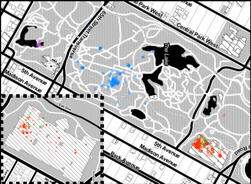
Figure 1: Tweet locations for four spatiotemporal patterns inferred by the SDHP. The underlying collective social activities correspond to a typical visit to the Metropolitan Museum of Art (the Met; in red), journalists tweeting at a press preview at the Met (in green), a typical visit to Gapstow Bridge (in purple), and musical concerts held at Rumsey Playfield and Naumburg Bandshell (in blue). Each circle corresponds to a tweet.

3 Preliminaries

In this section, we review the three major building blocks of the Spatial Dirichlet Hawkes Process (SDHP): the Dirichlet Process [6], the Hawkes Process [18], and the Normal distribution under the Normal-Gamma prior [23].

3.1 Dirichlet Process

The Dirichlet process $DP(\beta,G_{0})$ is a well known Bayesian nonparametric prior, parametrized by a concentration parameter $\beta>0$ and a base distribution $G_{0}(\theta)$ over a given space $\theta\in\Theta$. A sample $G\sim DP(\beta,G_{0})$ drawn from a DP is a discrete distribution. One can generate samples from a DP using a generative process called the Chinese Restaurant Process (CRP). The CRP assumes a Chinese restaurant with an infinite number of tables, each corresponding to a cluster, so that whenever a new customer arrives, she can either choose an existing table $k$ with $m_{k}$ seated customers or sit at an empty table. More specifically, one can obtain samples from the DP as follows:

• Assign the first customer to an empty table and draw its parameter $\theta_{1}$ from $G_{0}$.

• For $n>1$:

  • With probability $\frac{\beta}{\beta+n-1}$ assign customer $n$ to an empty table and draw $\theta_{n}$ from $G_{0}$.

  • With probability $\frac{m_{k}}{\beta+n-1}$ assign customer $n$ to the non-empty table $k$ and reuse $\theta_{k}$ for $\theta_{n}$.

Since a new cluster can be created at each step with non-zero probability, the number of clusters is potentially infinite and thus the process can adapt to increasing complexity in the data.

3.2 Hawkes Process

A Hawkes process is a type of temporal point process [1], which is a stochastic process whose realization consists of a sequence of discrete events localized in time, $\mathcal{H}=\left\{t_{i}\in\mathbb{R}^{+}\,|\,t_{i}<t_{i+1}\right\}$. A temporal point process can also be represented as a counting process via $N(t)$, which is the number of events up to time $t$. Moreover, we can characterize the counting process using the conditional intensity function $\lambda^{*}(t)$, which is the conditional probability of observing an event in an infinitesimal time window $[t,t+dt)$ given the history $\mathcal{H}(t)=\{t_{i}\in\mathcal{H}\,|\,t_{i}<t\}$, i.e.

$$\mathbb{E}[dN(t)|\mathcal{H}(t)]=\mathbb{P}\left\{\text{event in $[t,t+dt)|\mathcal{H}(t)$}\right\}=\lambda^{*}(t)dt$$

where $dN(t)\in\{0,1\}$. In the case of Hawkes processes, the intensity function takes the form

$$\lambda^{*}(t)=\lambda_{0}+\!\!\!\sum_{t_{i}\in\mathcal{H}(t)}\!\!\gamma(t,t_{i})$$ (1)

where $\lambda_{0}$ is the base intensity and $\gamma(\cdot)$ is the triggering kernel. Hawkes processes have been increasingly used to model social activity [16, 27], since they are able to capture mutual excitation between events and thus open up the possibility of modeling bursts of rapidly occurring events separated by long periods of inactivity [7].

3.3 Normal distributions with unknown mean and variance

A conjugate prior for normally distributed data with unknown mean and variance, $x\sim\mathcal{N}(\cdot|\mu,\sigma)$, is the normal-gamma prior given by

$$\mathcal{N}(\mu|\mu_{0},(\kappa_{0}\lambda)^{-1})\;{\rm Ga}(\lambda|\alpha_{0},\beta_{0})$$ (2)

where $\lambda\equiv 1/\sigma^{2}$.

4 Proposed Model

In this section we build on the above and formulate our model for clustering streaming spatiotemporal data, the Spatial Dirichlet Hawkes Process (SDHP). We first describe the geolocated posts it is designed to model, then elaborate on the different pieces used to model the time, content and location of each post, and finally introduce a generative process view of the model.

4.1 Geolocated post data

Given an online social network or media site, we represent each geolocated post created by a user as a tuple $(t,\mathbf{d},\mathbf{r},s)$, where $t$ is the time when the post was posted, $\mathbf{d}$ is the post content, $\mathbf{r}$ is the location (e.g. latitude, longitude) from where the user posted the post, and $s$ is the associated spatiotemporal pattern, which is latent. Throughout we will use $N$ to denote the number of posts in a given dataset $\mathcal{D}$.

4.2 Intensity functions

The time $t$ associated to each geolocated post is drawn from a Hawkes process with intensity given by

$$\lambda(t)=\lambda_{0}+\sum_{s}\lambda_{s}(t)$$ (3)

where the constant $\lambda_{0}$ is the base intensity and where the pattern-specific intensity is given by

$$\lambda_{s}(t_{n})=\sum_{i=1}^{n-1}\gamma_{s_{i}}(t_{n},t_{i})\mathbb{I}(s_{i}=s)$$ (4)

and $\gamma_{s}(t,t_{i})=\alpha_{s}e^{-(t-t_{i})/\tau_{s}}$ is an exponential triggering kernel. Here, the self-excitation parameter $\alpha_{s}$ and the time constant $\tau_{s}$ depend on the spatiotemporal pattern $s$. We assume that $\alpha_{s}$ is sampled from ${\operatorname{Ga}}(\alpha_{\rm time},\beta_{\rm time})$ and that $\tau_{s}$ is drawn from a uniform prior.

4.3 Content Distribution

The content associated to each geolocated post is represented by a vector $\mathbf{d}$ in which each element is a word sampled from a vocabulary $\mathcal{V}$ as

$$d_{j}\sim\rm{Multinomial}(\bm{\theta}_{s})$$ (5)

where $\bm{\theta}_{s}$ is a $|\mathcal{V}|$-length vector whose elements encode each word probability and which depends on the spatiotemporal pattern $s$ that the post belongs to. For each spatiotemporal pattern we assume $\bm{\theta}_{s}$ is sampled from $\operatorname{Dirichlet}(\theta_{0})$.

4.4 Spatial Distribution

The spatial location associated to each geolocated post is represented by a 2-dimensional vector $\mathbf{r}=(x,y)$, which is drawn from a normal distribution, i.e.

$$\mathbf{r}\sim\mathcal{N}(\mathbf{R}_{s},\mathbf{\Sigma}_{s})$$ (6)

where the mean and covariance depend on the spatiotemporal pattern $s$ the post belongs to. Here, we consider isotropic distributions with $\mathbf{\Sigma}_{s}=\sigma_{s}^{2}\mathbf{I}$ and assume that for each spatiotemporal pattern $s$ the mean $\mathbf{R}_{s}$ is drawn from a flat (improper) prior and $\sigma_{s}^{2}$ is drawn from ${\operatorname{Inv-Ga}}(1,\beta_{\rm space}^{-1})={\operatorname{Inv-Exp}(\beta_{\rm space}^{-1})}$. The conjugacy of these priors will be crucial in designing an efficient inference procedure in Section 5.

4.5 Generative Process

In the previous sections we assumed that the spatiotemporal pattern a post belongs to is given and then modeled the time, content, and location of the post using conditional distributions whose parameters depend on the associated pattern. Next we introduce a generative process—inspired by the Chinese Restaurant Process—in which posts are assigned to spatiotemporal patterns as they are generated:

• Initialize the number of patterns: $S\to 0$.

• For $n=1,\ldots,N$:

  • Sample $t_{n}$ from Poisson($\lambda_{0}+\sum_{i=1}^{n-1}\gamma_{s_{i}}(t_{n},t_{i})$)
    

  • • Assign post $n$ to a new spatiotemporal pattern $s_{n}=S+1$ with probability

      $$\frac{\lambda_{0}}{\lambda_{0}+\sum_{i=1}^{n-1}\gamma_{s_{i}}(t_{n},t_{i})},$$

      draw its associated parameters $(\bm{\theta}_{s_{n}},\mathbf{R}_{s_{n}},\sigma_{s_{n}}^{-2})$ from the corresponding priors, and increase the number of patterns $S\to S+1$.

    • If post $n$ is not assigned to a new pattern in step (i) above, then with probability

      $$\frac{\lambda_{k}(t_{n})}{\lambda_{0}+\sum_{i=1}^{n-1}\gamma_{s_{i}}(t_{n},t_{i})},$$

      assign it to an existing spatiotemporal pattern $s_{n}=k$, where $k=1,\ldots,S$ and $\lambda_{k}(t_{n})=\sum_{i=1}^{n-1}\gamma_{s_{i}}(t_{n},t_{i})\mathbb{I}(s_{i}=k)$ and reuse $(\bm{\theta}_{k},\mathbf{R}_{k},\sigma_{k})$.
      

  • Sample $\mathbf{d}_{n}$ from $\rm{Multinomial}(\bm{\theta}_{s_{n}})$ and $\bm{r}_{n}$ from $\mathcal{N}(\mathbf{R}_{s_{n}},\sigma_{s_{n}}^{2}\mathbf{I})$.

Note that the base intensity $\lambda_{0}$ controls the rate at which new patterns are created.

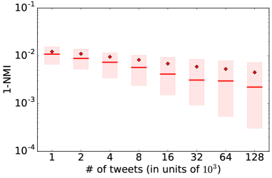
(a) Accuracy of spatiotemporal pattern inference

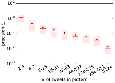
(b) Estimation of $\alpha_{s}$

Figure 2: Accuracy of our inference algorithm. Panel (a) shows the normalized mutual information (NMI) as a function of the number of tweets fed into the inference algorithm. Inferential accuracy remains high as the size of the dataset increases. Panel (b) shows how the precision with which the self-excitation parameter $\alpha_{s}$ can be inferred increases as the number of observed tweets per inferred pattern increases. For both figures the diamonds mark the mean and the thick lines mark the mode, while each box extends from the lower to upper quartile.

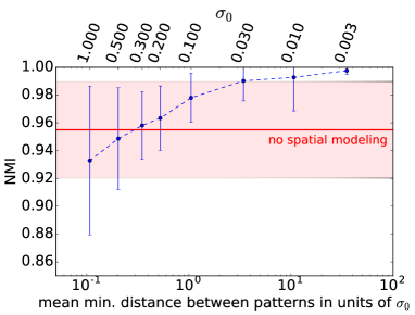
(a) NMI vs. $\sigma_{0}$

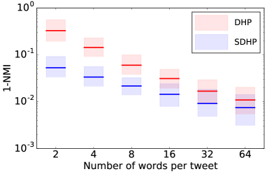
(b) SDHP vs. DHP

Figure 3: To what extent does spatial information help during inference? Results for the SDHP are in blue, while results for the DHP are in red. Panel (a) shows the mean normalized mutual information (NMI) with standard errors as a function of the true spatial variance $\sigma_{0}^{2}$ of the generated spatiotemporal patterns (top axis) as well as a function of a measure of spatial overlap (bottom axis). Panel (b) shows $1-$NMI as a function of the number of words per tweet. Thick lines denote the mode, while each box stretches from the lower to upper quantile.

5 Inference

Given a collection of $N$ observed geolocated posts generated by the users of an online social network or media site during a time period $[0,T)$, our goal is to infer the spatiotemporal patterns that these posts belong to. To efficiently sample from the posterior distribution, we derive a sequential Monte Carlo (SMC) algorithm [17, 14] that exploits the temporal dependencies in the observed data to sequentially sample the latent variables associated to each geolocated post. The runtime of the algorithm is $\mathcal{O}(N\!\!\times\!\!|\mathcal{P}|\!\!\times\!\!\bar{S})$, where $|\mathcal{P}|$ is the number of particles used during SMC and $\bar{S}$ is the mean number of latent spatiotemporal patterns. For a detailed description of the algorithm please refer to the appendix.

6 Experiments on Synthetic Data

In this section we examine the performance of our inference algorithm under a variety of conditions using synthetic data drawn from the generative process.

6.1 Experimental Setup

Each of the synthetic experiments described below has the same structure. All parameters but one—call it $x$—are kept fixed in each experiment, while for each value of $x$ a large number of trials is done, with each trial running the (S)DHP inference algorithm on a sample drawn from the generative process. Reported are summary statistics for each set of trials corresponding to each value of $x$.

6.2 Results

We first evaluate the performance of our inference algorithm as the number of geolocated tweets in each sample as well as the number of tweets per inferred pattern increases. Figure 2 summarizes the results, which show that: (i) the assignment of tweets to spatiotemporal patterns, measured by means of the normalized mutual information (NMI) between the true and inferred spatiotemporal patterns, remains accurate for large datasets; and (ii) the estimation of the self-excitation parameters $\alpha_{s}$, as measured by the precision

$$\delta_{\alpha}=\tfrac{|\alpha_{s}-\hat{\alpha}_{s}|}{|\alpha_{s}+\hat{\alpha}_{s}|/2}$$

becomes more accurate as the size of inferred patterns increases, as expected.

Next we evaluate the extent to which our inference algorithm benefits from the spatial information contained in each geolocated tweet. Intuitively, the smaller the spatial variance of a given pattern $s$, the more informative the spatial information of the tweets belonging to $s$ should be. Figure 3a confirms this intuition by showing the NMI as a function of the spatial variance $\sigma_{0}^{2}$ of the generated patterns. As $\sigma_{0}$ decreases (so that the spatial overlap between different patterns decreases) the inferential accuracy of the SDHP increases and surpasses that of the DHP [15]. Moreover, Figure 3b shows that spatial information becomes more valuable when the associated content is less informative by comparing the NMI achieved by SDHP (in blue) and by the DHP (in red) for a varying number of words per tweet.

7 Experiments on Real Data

In this section, we apply our model to real world data from Twitter. First, we show that our model recovers meaningful spatiotemporal patterns across a diverse range of spatial and temporal scales. Then we demonstrate that the SDHP can be used to perform accurate prediction of tweet locations, performing favorably with respect to two baselines [15, 19]. Finally we perform a quantitative evaluation of spatial and content goodness of fit in comparison to two baselines.

7.1 Experimental Setup

Our data consist of the time, location and content of $12{,}558{,}046$ geolocated tweets posted during a one year period from January 1, 2013 to December 31, 2013 in a bounding box spanning Manhattan, New York City. In this work, we focus on tweets written in English, as determined by the language tags provided by GNIP, and create two datasets: (i) $\mathcal{D}_{1}$, which includes $|\mathcal{D}_{1}|=3{,}695{,}301$ tweets posted from Manhattan south of Central Park; and (ii) $\mathcal{D}_{2}$, which includes $|\mathcal{D}_{2}|=69{,}538$ tweets posted from Central Park. Finally, we preprocess the tweet content as follows: (i) all words are made lowercase; (ii) the $200$ most frequent words in the entire sample are filtered out; and (iii) punctuation/hashtags are left as is.

7.2 Spatiotemporal patterns

In this section, we perform a qualitative analysis of the spatiotemporal patterns picked out by the SDHP. To this end we run our inference algorithm on the Central Park dataset $\mathcal{D}_{2}$, which reveals $7{,}639$ spatiotemporal patterns. Here we choose the hyperparameters by cross-validation on a held-out set and use the set of time constants $\Psi_{\tau}=\{{\rm hour},{\rm day},{\rm week},{\rm month},{\rm quarter\mathchar 45\relax year},{\rm year}\}$.

First we examine the spatiotemporal characteristics of the revealed spatiotemporal patterns at an aggregate level. Intuitively, since Central Park encompasses a relatively large area where a variety of collective social activities are undertaken (e.g. concerts, picnicking, sports, etc.), we expect to find patterns spanning a diverse range of spatial and temporal scales. Figure 4 summarizes the results, which shows that the SDHP picks out spatiotemporal patterns with a diverse range of pattern sizes (from a few tweets to hundreds), spatial extent (from $\sigma<5$ to $\sigma>1000$ meters), and time constants (from $\tau=$ hour to $\tau=$ month).

Next we examine the content for patterns spanning different temporal and spatial scales. To do so we group the inferred spatiotemporal patterns into four sets based on their spatial extent ($\sigma\lessgtr 100$m) and their time duration ($\Delta t\lessgtr 1$ week). Then for each set we create a word cloud that encodes the ten most frequent terms in the set, see Figure 5. Remarkably, the most popular words in each set reflect the underlying spatiotemporal characteristics. For example, the spatiotemporal patterns that are localized in time ($\Delta t<1$ week) often correspond to specific events which take place at specific locations in the park (e.g. summer stage for $\sigma<100$m) as well as throughout the entire park (e.g. the NYC Marathon for $\sigma>100$m); spatiotemporal patterns that unfold over longer periods of time ($\Delta t\geq 1$ week) often include words describing static features of Central Park such as ‘strawberry’ and ‘fields’ for $\sigma<100$m, referring to a small memorial dedicated to John Lennon, or ‘reservoir’ and ‘lake’ for $\sigma\geq 100$m.

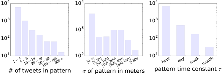
Figure 4: The distribution of pattern sizes inferred across the entire dataset $\mathcal{D}_{2}$ in terms of number of tweets (left) and spatial extent in meters (middle). Also plotted (right) is the distribution of the time constants $\Psi_{\tau}$; note that none of the inferred patterns is assigned $\tau=$ quarter-year or $\tau=$ year.

Finally we turn to examine the spatiotemporal characteristics of four individual patterns more closely: a typical visit to the Metropolitan Museum of Art (the Met), a press preview to an exhibition at the Met, a typical visit to the iconic Gapstow Bridge, and musical concerts held throughout the summer at Rumsey Playfield and Naumburg Bandshell. Figure 1 shows the location of the tweets assigned to each spatiotemporal pattern, and Figure 6 shows the content and temporal dynamics of each pattern by means of word clouds and fitted temporal intensities. In terms of spatial dynamics, the collective social activities span a wide range, from $\sigma\approx 8$m for visits to Gapstow Bridge to $\sigma\approx 100$m for the summer concerts. For the temporal dynamics, we find similar diversity, from $\alpha=25.97$ and $\Delta t\approx 2$ days for the press preview to $\alpha=1.01$ and $\Delta t\approx 91$ days for the summer concerts.

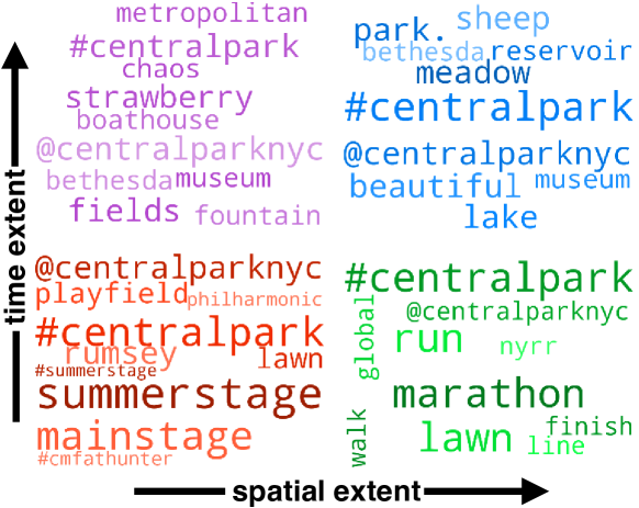
Figure 5: Four word clouds showing how the content of inferred patterns varies according to their time duration (less than or greater than 1 week) and their spatial extent (less than or greater than 100 meters).

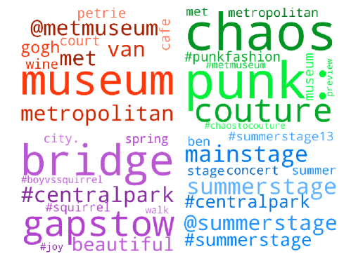
(a) Content

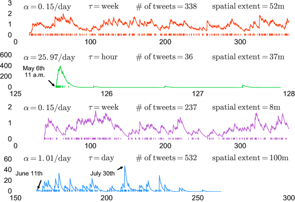
(b) Temporal Dynamics

Figure 6: Content and temporal dynamics of the four spatiotemporal patterns depicted in Figure 1. Panel (a) shows the word content of each pattern. Panel (b) shows the temporal dynamics for each pattern by means of the fitted intensities $\lambda_{s}(t)$ in units of inverse days and includes additional pattern-level summary statistics. Blips along the time axis correspond to individual tweets. The time axis is in units of days, while the pattern-specific intensities are in units of inverse days.

7.3 Location Prediction

We evaluate the performance of our model at predicting the location of tweets using dataset $\mathcal{D}_{1}$, which corresponds to tweets in Manhattan south of Central Park. We compare the performance of the SDHP in this context against two baselines: Bayesian Hierarchical Clustering (BHC) and the Dirichlet-Hawkes Process (DHP) [15]. Note that although the SHDP was not specifically designed for the purpose of tweet location prediction—rather it was designed to discover spatiotemporal patterns more broadly—we expect that if the assumptions underlying the spatial modeling are appropriate to the given dataset, then the SDHP should be able to make reasonable location predictions.

In this section, our focus is on tweets that belong to spatiotemporal patterns with sufficiently tight spatial structure such that the locations of the corresponding tweets are predictable. To this end, we will experiment with five subsets of length $2{,}500$ tweets, built by filtering on a fixed lists of keywords: ‘gallery’, ‘park’, ‘concert’, ‘sports’, and ‘bar’. Note that despite the potential for tight spatial structure of the underlying patterns suggested by the chosen keywords, the tweets within each subset are spread throughout Manhattan, as shown in Figure 7. For example, in the case of ‘gallery’, which represents the most concentrated sample of tweets, while there is a large cluster of galleries in Chelsea, there are also many galleries in SoHo, the Lower East Side, Midtown, and elsewhere. This, combined with the fact that an individual gallery may receive only a handful of—or even a single—mentions makes the prediction task difficult.

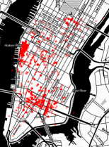
(a) Gallery

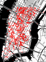
(b) Bar

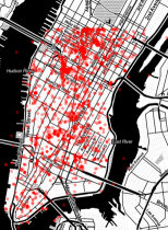
(c) Concert

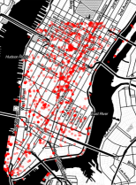
(d) Park

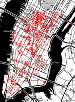
(e) Sports

Figure 7: Locations of the tweets in the five subsets of dataset $\mathcal{D}_{2}$ defined by the keywords ‘gallery’, ‘bar’, ‘concert’, ‘park’, and ‘sports’, respectively, that are used in the experiments in Sec. 7.3 and Sec. 7.4.

For each subset, we proceed as follows:

• We hide the location of 2% of the tweets, picked at random, excluding the first (chronologically) 20% of the tweets (burn-in period).

• We run the corresponding inference algorithm.

• We infer the position of each hidden tweet via its spatial posterior, which is just the mean location of the other (non-hidden) tweets in the spatiotemporal pattern the tweet is assigned to.

• We repeat steps $1$-$3$ for $100$ trials. If a tweet is hidden in more than one trial, we infer its position using the trial in which it is assigned to the tightest pattern (lower $\sigma_{s}$).

In the above procedure, we set the hyperparameters of all methods using a held-out validation set built using the ‘gallery’ subset and set $\Psi_{\tau}=\{{\rm hour},{\rm day},{\rm week},{\rm month},{\rm quarter\mathchar 45\relax year}\}$.

Then we evaluate the performance of each modeling framework using the root mean square error (RMSE), applying two different selection criteria that consider only location predictions about which the corresponding modeling framework is reasonably certain (see appendix for details).

Table 2 summarizes the results by means of the RMSE in units of the square root of the spatial variance of the entire subset of tweets, which ranges from $\sim\!\!1370$m in the case of ‘gallery’ to $\sim\!\!1660$m in the case of ‘park’. For most of the samples and both of the selection criteria, SDHP gives better location predictions than the two baselines. The accuracy of the prediction, however, varies significantly from sample to sample, as the difficulty of the task varies substantially depending on the keyword. Note that in the case of ‘concert’ too few tweets pass the tight selection criteria for the measure to be computed.

7.4 Goodness of fit

	loose selection			tight selection
keyword	SDHP	DHP	BHC	SDHP	DHP	BHC
gallery	0.056	0.087	0.068	0.167	0.047	0.013
park	0.051	0.055	0.111	0.040	0.057	0.134
concert	0.080	0.088	0.132	—	—	—
sports	0.247	0.388	0.429	0.289	0.600	0.449
bar	0.063	0.021	0.134	0.029	0.239	0.145

Table 1: Results for tweet location prediction.

	spatial goodness of fit mean log probability		content goodness of fit perplexity per word
keyword	SDHP	GMM	SDHP	DHP
gallery	6.26	9.15	$\mathbf{4.86\times 10^{4}}$	5.36$\times 10^{4}$
park	5.64	8.84	$\mathbf{12.1\times 10^{4}}$	$16.0\times 10^{4}$
concert	2.96	6.77	18.6$\times 10^{4}$	$\mathbf{18.0\times 10^{4}}$
sports	3.88	8.77	$\mathbf{10.3\times 10^{4}}$	10.9$\times 10^{4}$
bar	4.17	6.25	$\mathbf{16.3\times 10^{4}}$	18.3$\times 10^{4}$

Table 2: Results for goodness of fit tests.

We evaluate the goodness of fit of the SDHP at modeling collective social activity both in terms of spatial and content dynamics using the five subsets of dataset $\mathcal{D}_{1}$ described in Sec. 7.3. In terms of spatial dynamics, we compare the SDHP to a Gaussian Mixture Model (GMM), while in terms of content dynamics, we compare the SDHP to the Dirichlet Hawkes Process (DHP). In both cases the goodness of fit measure is a form of mean marginal log likelihood (see the appendix for details). Table 2 summarizes the results for both goodness of fit tests.

We see that for all five keywords the SDHP lags behind the GMM in the goodness of the spatial fit, but that the SDHP still provides a reasonable fit. This is as expected, since the SDHP also pays close attention to temporal and content dynamics; e.g. as we saw in Figure 1 in the case of the two patterns located at the Met, the SDHP will tend to model a given spatial cluster with multiple patterns if they have varying temporal/content characteristics, while the GMM will prefer a sparser representation and use the additional gaussian component(s) to improve the fit elsewhere.

For the content goodness of fit we see that the SDHP outperforms the DHP in four out of five samples (underperforming only for the keyword with the lowest spatial goodness of fit, namely ‘concert’). This is encouraging, as it demonstrates that utilizing spatial information allows the SDHP to a provide a more faithful content model for real world data.

8 Conclusions

We proposed a novel continuous spatiotemporal probabilistic model for clustering streaming geolocated data, the Spatial Dirichlet Hawkes Process (SDHP), and developed an efficient, online inference algorithm based on sequential Monte Carlo that scales to millions of posts. We showcased the efficacy of the model on data from Twitter and demonstrated that it can reveal a wide range of spatiotemporal patterns underlying different collective social activities. In this application domain our model provides a better fit to the content dynamics of the data as well as more accurate location predictions than several alternatives [19, 15].

Our work opens up many interesting avenues for future work. For example, we consider isotropic distributions to model the spatial dynamics of each pattern; however, there are many scenarios (e.g. traffic jams) in which other distributions may be more appropriate. It would also be valuable to augment our model to have a hierarchical design in which there are canonical spatiotemporal patterns (e.g. traffic jams) with different spatial distributions that are then instantiated at different points in time and space. In addition it would be interesting to apply our model to other sources of geolocated data, such as cellular phone data, mobile messaging data (e.g. Whatsapp or Snapchat), or mobile photo-sharing data (e.g. Instagram).

More broadly it could be useful to integrate our model into a larger information extraction pipeline, especially in the context of extracting insights from urban social media data for the use of local government. For example, one could design a system that assists local prosecutors in identifying possible cases of consumer fraud and tenant harassment. Finally, whereas we have focused on collective social activities, it would be instructive to use the SDHP in the context of spatiotemporally localized events, especially in the context of crisis and disaster awareness [21].

9 Appendix

9.1 Details on Inference Algorithm

In this subsection we describe how Sequential Monte Carlo can be used to infer latent patterns from the observed spatiotemporal and content data. The posterior distribution $p(s_{1:n}|t_{1:n},\mathbf{d}_{1:n},\mathbf{r}_{1:n})$ is sequentially approximated from $n=1$ to $n=N$ with a set of $|\mathcal{P}|$ particles that are sampled from a proposal distribution that factorizes as

$$q_{n}(s_{\leq n}|t_{\leq n},\mathbf{d}_{\leq n},\mathbf{r}_{\leq n}) =q_{n}(s_{n}|s_{<n},t_{\leq n},\mathbf{d}_{\leq n},\mathbf{r}_{\leq n})$$

$$\times q_{n-1}(s_{<n}|t_{<n},\mathbf{d}_{<n},\mathbf{r}_{<n})$$

where $q_{n}(s_{n}|s_{<n},t_{\leq n},\mathbf{d}_{\leq n},\mathbf{r}_{\leq n})$ is given by

$$\frac{p(s_{n}|s_{<n},t_{\leq n})p(\mathbf{d}_{n}|s_{\leq n},\mathbf{d}_{<n})p(\mathbf{r}_{n}|s_{\leq n},\mathbf{r}_{<n})}{\sum_{s_{n}}p(s_{n}|s_{<n},t_{\leq n})p(\mathbf{d}_{n}|s_{\leq n},\mathbf{d}_{<n})p(\mathbf{r}_{n}|s_{\leq n},\mathbf{r}_{<n})}$$ (7)

In the above expression, the distribution $p(s_{n}|s_{<n},t_{\leq n})$ is given by

$$p(s_{n}|s_{<n},t_{\leq n})=\frac{\lambda_{s_{n}}(t_{n})}{\lambda_{0}+\sum_{i=1}^{n-1}\gamma_{s_{i}}(t_{n},t_{i})}$$ (8)

where the numerator $\lambda_{s_{n}}(t_{n})$ is equal to $\lambda_{0}$ when $s_{n}$ is a new spatiotemporal pattern.

We can exploit the conjugacy between the multinomial and the Dirichlet distributions as well as the conjugacy between the normal distribution and normal-gamma prior to integrate out the word distributions $\bm{\theta}_{s}$ and spatial parameters $\{\sigma_{s},\mathbf{R}_{s}\}$, respectively, and obtain the marginal likelihoods:

$$p(\mathbf{d}_{n}|s_{\leq n},\mathbf{d}_{<n})=\frac{\Gamma({C^{s_{n}/\ \!\!\mathbf{d}_{n}}}\!+\!V\theta_{0})\prod_{v}^{V}\!\Gamma({C^{s_{n}/\ \!\!\mathbf{d}_{n}}_{v}}\!+\!{C^{\mathbf{d}_{n}}_{v}}\!+\!\theta_{0})}{\Gamma({C^{s_{n}/\ \!\!\mathbf{d}_{n}}}\!+\!{C^{\mathbf{d}_{n}}}\!+\!V\theta_{0})\prod_{v}^{V}\!\Gamma({C^{s_{n}/\ \!\!\mathbf{d}_{n}}_{v}}\!+\!\theta_{0})}$$

where $V$ is the size of the observed vocabulary, ${C^{s_{n}/\ \!\!\mathbf{d}_{n}}}$ is the total number of words in the spatiotemporal pattern $s_{n}$ seen so far excluding $\mathbf{d}_{n}$, ${C^{s_{n}/\ \!\!\mathbf{d}_{n}}_{v}}$ is the total count for word $v$ in spatiotemporal pattern $s_{n}$ so far excluding $\mathbf{d}_{n}$, $C^{\mathbf{d}_{n}}_{v}$ is the total count for word $v$ in $\mathbf{d}_{n}$ and $C^{\mathbf{d}_{n}}$ is the total word count for $\mathbf{d}_{n}$; and,

$$p(\mathbf{r}_{n}|s_{\leq n},\mathbf{r}_{<n})=\begin{cases}\frac{N_{s_{n}}^{2}}{2\pi(1+N_{s_{n}})}\frac{\xi_{s_{n}}^{-1}}{[1+\Delta(\mathbf{r}_{n})/\xi_{s_{n}}]^{1+N_{s_{n}}}}&\!\!\text{if}\;N_{s_{n}}\!\geq\!1\\ 1&\!\!\text{if}\;N_{s_{n}}\!=\!0\end{cases}$$

where $N_{s_{n}}=\sum_{i=1}^{n-1}\mathbb{I}[s_{i}=s_{n}]$ is the number of posts assigned to spatiotemporal pattern $s_{n}$, $\xi_{s_{n}}$ is given by

$$\xi_{s_{n}}=\beta_{\rm space}+\tfrac{1}{2}\sum_{i=1}^{n-1}\mathbf{r}_{i}^{2}\mathbb{I}[s_{i}=s_{n}]-\tfrac{1}{2N_{s_{n}}}\left(\sum_{i=1}^{n-1}\mathbf{r}_{i}\mathbb{I}[s_{i}=s_{n}]\right)^{2}$$

​and

$$\Delta(\mathbf{r}_{n})=\frac{N_{s_{n}}}{2(N_{s_{n}}+1)}\left(\mathbf{r}_{n}-\frac{1}{N_{s_{n}}}\sum_{i=1}^{n-1}\mathbf{r}_{i}\mathbb{I}[s_{i}=s_{n}]\right)^{2}$$

This choice of $q_{n}(\cdot)$ results in the incremental importance weight

$$\alpha_{n}(s_{<n})=p(t_{n}|s_{<n},t_{<n})Q_{n}(s_{<n},t_{\leq n},\mathbf{d}_{\leq n},\mathbf{r}_{\leq n})$$ (9)

where $Q_{n}(s_{<n},t_{\leq n},\mathbf{d}_{\leq n},\mathbf{r}_{\leq n})$ is given by

$$\sum_{s_{n}}p(s_{n}|s_{<n},t_{\leq n})p(\mathbf{d}_{n}|s_{\leq n},\mathbf{d}_{<n})p(\mathbf{r}_{n}|s_{\leq n},\mathbf{r}_{<n})$$ (10)

This update is optimal in the sense that it leads to minimum variance among the particle weights. Finally note that in order to mitigate against particle degeneracy systematic resampling is used whenever the particle system satisfies $\|\textrm{\bf w}_{n}\|_{2}^{-2}<\kappa_{\rm thresh}|\mathcal{P}|$ (throughout we use $\kappa_{\rm thresh}=0.9$). For more details on Sequential Importance Resampling see e.g. ref. [14].

1 Initialize $w^{(p)}_{1}\to 1/|\mathcal{P}|$ and $S^{(p)}\to 0$ for all $p\in\mathcal{P}$.

2 for $n=1,\ldots,N$ do

3       for $p\in\mathcal{P}$ do

4             Draw $s^{(p)}_{n}$ from Eqn. 7.

5            if $s^{(p)}_{n}=S^{(p)}+1$ then

6                   Draw the time kernel parameters $\{\alpha_{s},\tau_{s}\}$ for $s={s^{(p)}_{n}}$ from the prior

7                  

8                   Increase the number of patterns $S^{(p)}\to S^{(p)}+1$

9                  

10            Update the particle weight $\textrm{w}^{(p)}_{n}$ using Eqn. 9

11             Update $\{\alpha_{s},\tau_{s}\}$ for all patterns via Eqn. 12

12            

13      Normalize particle weights.

14       if $\|\textrm{\bf w}_{n}\|_{2}^{-2}<\kappa_{\rm thresh}|\mathcal{P}|$ then

15             Resample particles.

16      

Finally return the particle $p\in\mathcal{P}$ with the largest weight as an approximate MAP estimate to Eqn. 11.

Algorithm 1 Inference algorithm for the SDHP

9.1.1 Time kernel inference

If the time kernels parameters, $\{\alpha_{s},\tau_{s}\}$, are fixed the inference procedure described above yields an unbiased estimate of the posterior $p(s_{1:N}|t_{1:N},\mathbf{d}_{1:N},\mathbf{r}_{1:N})$. In general, however, these parameters are unknown and need to be estimated. Methods for calculating the full posterior $p(s_{1:N},\{\alpha_{s},\tau_{s}\}|t_{1:N},\mathbf{d}_{1:N},\mathbf{r}_{1:N})$ can be derived; however, they are computationally expensive and do not scale to large datasets (since they rely on e.g. expensive MCMC updates). Since our primary interest is not in the posterior itself but rather the MAP estimate, i.e.

$$s_{1:N}^{\rm MAP}=\underset{s_{1:N}}{\arg\max}\;p(s_{1:N}|t_{1:N},\mathbf{d}_{1:N},\mathbf{r}_{1:N}),$$ (11)

we do not necessarily require SMC to produce unbiased samples from the posterior. Rather, we just need SMC to explore the posterior space efficiently and return an (approximate) MAP estimate. Consequently, we use the following computationally efficient procedure: after each time step, the parameters $\{\alpha_{s},\tau_{s}\}$ are set equal to a (restricted) MLE estimate. More specifically, as part of the model specification we choose a fixed, finite set of allowed time constants, $\Psi_{\tau}=\{\tau_{i}\}$. Then at each time step $n$ and for each spatiotemporal pattern $s$ and $\tau_{i}\in\Psi_{\tau}$ we compute

$$\alpha_{s}^{\rm MLE}(\tau_{i})=\underset{\alpha_{s}}{\arg\max}\;p(\alpha_{s}|\alpha_{\rm time},\beta_{\rm time})p(\mathcal{T}_{s;n}|\alpha_{s},\tau_{i})$$ (12)

where $\mathcal{T}_{s;n}$ is the sequence of times for the posts assigned to spatiotemporal pattern $s$ through time step $n$. For each $\tau_{i}\in\Psi_{\tau}$ Eqn. 12 can be computed in closed form. Finally, we choose the pair $(\alpha_{s}^{\rm MLE}(\tau_{i}),\tau_{i})$ that maximizes the likelihood in Eqn. 12. In this way the parameters $\{\alpha_{s},\tau_{s}\}$ are updated at each time step for all patterns that contain at least two posts.

9.2 Setup for synthetic experiments

Unless stated otherwise, the following experimental parameters are common to all four experiments: the vocabulary has length $|\mathcal{V}|=15$; the hyperparameters for the prior on the self-excitation parameter $\alpha_{s}$ are given by $\alpha_{\rm time}=0.1$ and $\beta_{\rm time}=0.2$; the base intensity $\lambda_{0}=10$; the time constants are given by $\Psi_{\tau}=\{1\}$; the Dirichlet hyperparameter is given by $\theta_{0}=1$; the number of words per tweet is given by $N_{\rm words}=7$; and the number of particles used during inference is $|\mathcal{P}|=4$. The number of tweets in each sample will be denoted as $N$ and the number of trials per value of $x$ will be denoted as $N_{\rm trials}$.

In order for the spatial part of the generative process to be well-defined, we use a uniform prior on the mean location $\mathbf{R}_{s}$ of each pattern $s$, with the prior defined on the unit square. Unless stated otherwise the spatial hyperparameter $\beta_{\rm space}=0.01$ and the generative process assigns each spatiotemporal pattern a spatial extent $\sigma_{0}=0.1$.

For the experiment corresponding to Fig. 2a we set $N_{\rm trials}=60$ and $\sigma_{0}=0.03$, while for the experiment corresponding to Fig. 2b we set $N=5500$ and $N_{\rm trials}=500$ as well as $N_{\rm words}=15$ and $\sigma_{0}=0.02$ (so that even smaller patterns should be readily identifiable). For the experiment corresponding to Fig. 3a we set $N=500$, $N_{\rm trials}=50$, $|\mathcal{P}|=8$, and $\beta_{\rm space}=\sigma_{0}^{2}$, while for the experiment corresponding to Fig. 3b we set $N=2000$, $N_{\rm trials}=200$, $\sigma_{0}=0.03$, and $|\mathcal{P}|=1$.

9.3 Details on Location Prediction Experiment

The two selection criteria used in the paper are defined as follows:

— Loose selection: we sort all tweets in ascending order according to the $\sigma_{s}$ of the associated pattern, discard any tweet in a pattern with less than $7$ tweets, and compute the average root mean square error (RMSE) of the top 4%.

— Tight selection: we sort all tweets in ascending order according to the $\sigma_{s}$ of the associated pattern, discard any tweet in a pattern with less than $11$ tweets, and compute the average root mean square error (RMSE) of the top 4%.

In the above measures, ties are adjudicated by preferring tweets which belong to patterns with more tweets. Any remaining ties are decided randomly.

9.4 Goodness of Fit Measures

9.4.1 Spatial measure

We use the following spatial goodness of fit measure. At each iteration $n$ of the corresponding inference algorithm (after a burnin period of 500 tweets), we evaluate the marginal likelihood of the next sample $n+1$ given the parameters and latent variables inferred from the first $n$ samples; e.g. for the SDHP we have:

$$\!{\rm spatial\;g.o.f.}=\tfrac{1}{2000}\!\!\sum_{n=501}^{2500}\!\!\log p(\bm{r}_{n}|t_{\leq n},s_{<n},\bm{d}_{\leq n},\bm{r}_{<n})$$ (13)

An analogous expression (i.e. without conditioning on $\bm{d}_{\leq n}$ and $t_{\leq n}$) holds for the GMM. In order to make a more direct comparison between the two models we setup the GMM as follows: (i) at each iteration $n$ we set the number of gaussian components equal to the number of spatiotemporal patterns inferred by the SDHP at time step $n-1$; and (ii) we consider isotropic gaussians with the minimum covariance set equal to ${\sigma^{2}}_{\rm{min}}=2\beta_{\rm{space}}$.

9.4.2 Content measure

With reference to the expression in Eqn. 13, we use a related goodness of fit measure, namely the perplexity $\mathcal{P}$ [10]; e.g. for the DHP we have the following:

$$\mathcal{P}\!=\exp\!\left(\!\!\tfrac{-1}{N_{\rm{words}}}\!\!\sum_{n=501}^{2500}\!\!\log p(\bm{d}_{n}|t_{\leq n},s_{<n},\bm{d}_{<n})\!\right)$$

where $N_{\rm{words}}$ is the total number of words in $\{\bm{d}_{501},...,\bm{d}_{2500}\}$. An analogous expression (i.e. with additional conditioning on $\bm{r}_{\leq n}$) holds for the SDHP. In order to make a more direct comparison between the two models we set $\lambda_{0}$ for the DHP such that the number of inferred patterns matches that of the SDHP.

References

- [1] O. Aalen, O. Borgan, and H. K. Gjessing. Survival and event history analysis: a process point of view. Springer, 2008.
- [2] H. Abdelhaq, C. Sengstock, and M. Gertz. Eventweet: Online localized event detection from twitter. Proceedings of the VLDB Endowment, 6(12):1326–1329, 2013.
- [3] A. Ahmed, Q. Ho, J. Eisenstein, E. Xing, A. J. Smola, and C. H. Teo. Unified analysis of streaming news. In Proceedings of the 20th international conference on World wide web, pages 267–276. ACM, 2011.
- [4] A. Ahmed, Q. Ho, C. H. Teo, J. Eisenstein, E. P. Xing, and A. J. Smola. Online inference for the infinite topic-cluster model: Storylines from streaming text. In International Conference on Artificial Intelligence and Statistics, pages 101–109, 2011.
- [5] A. Ahmed and E. P. Xing. Dynamic non-parametric mixture models and the recurrent chinese restaurant process: with applications to evolutionary clustering. In SDM, pages 219–230. SIAM, 2008.
- [6] C. E. Antoniak. Mixtures of dirichlet processes with applications to bayesian nonparametric problems. The annals of statistics, pages 1152–1174, 1974.
- [7] A.-L. Barabási. The origin of bursts and heavy tails in human dynamics. Nature, 435:207, 2005.
- [8] R. Becker, R. Cáceres, K. Hanson, S. Isaacman, J. M. Loh, M. Martonosi, J. Rowland, S. Urbanek, A. Varshavsky, and C. Volinsky. Human mobility characterization from cellular network data. Communications of the ACM, 56(1):74–82, 2013.
- [9] D. M. Blei and P. I. Frazier. Distance dependent chinese restaurant processes. The Journal of Machine Learning Research, 12:2461–2488, 2011.
- [10] D. M. Blei, A. Y. Ng, and M. I. Jordan. Latent dirichlet allocation. The Journal of Machine Learning Research, 3:993–1022, 2003.
- [11] F. Chierichetti, J. M. Kleinberg, R. Kumar, M. Mahdian, and S. Pandey. Event detection via communication pattern analysis. In ICWSM, 2014.
- [12] E. Cho, S. A. Myers, and J. Leskovec. Friendship and mobility: user movement in location-based social networks. In Proceedings of the 17th ACM SIGKDD international conference on Knowledge discovery and data mining, pages 1082–1090, 2011.
- [13] Q. Diao and J. Jiang. Recurrent chinese restaurant process with a duration-based discount for event identification from twitter. In SDM, pages 388–397. SIAM, 2014.
- [14] A. Doucet and A. M. Johansen. A tutorial on particle filtering and smoothing: Fifteen years later. Handbook of Nonlinear Filtering, 12(656-704):3, 2009.
- [15] N. Du, M. Farajtabar, A. Ahmed, A. J. Smola, and L. Song. Dirichlet-hawkes processes with applications to clustering continuous-time document streams. In Proceedings of the 21th ACM SIGKDD International Conference on Knowledge Discovery and Data Mining, pages 219–228. ACM, 2015.
- [16] M. Farajtabar, N. Du, M. Gomez-Rodriguez, I. Valera, H. Zha, and L. Song. Shaping social activity by incentivizing users. In NIPS, 2014.
- [17] N. J. Gordon, D. J. Salmond, and A. F. Smith. Novel approach to nonlinear/non-gaussian bayesian state estimation. In Radar and Signal Processing, IEE Proceedings F, volume 140, pages 107–113. IET, 1993.
- [18] A. G. Hawkes. Spectra of some self-exciting and mutually exciting point processes. Biometrika, 58(1):83–90, 1971.
- [19] K. A. Heller and Z. Ghahramani. Bayesian hierarchical clustering. In Proceedings of the 22nd international conference on Machine learning, pages 297–304. ACM, 2005.
- [20] A. Ihler, J. Hutchins, and P. Smyth. Adaptive event detection with time-varying poisson processes. In Proceedings of the 12th ACM SIGKDD international conference on Knowledge discovery and data mining, pages 207–216, 2006.
- [21] M. Imran, S. M. Elbassuoni, C. Castillo, F. Diaz, and P. Meier. Extracting information nuggets from disaster-related messages in social media. Proc. of ISCRAM, Baden-Baden, Germany, 2013.
- [22] N. D. Lane, L. Pengyu, L. Zhou, and F. Zhao. Connecting personal-scale sensing and networked community behavior to infer human activities. In Proceedings of the 2014 ACM International Joint Conference on Pervasive and Ubiquitous Computing, pages 595–606, 2014.
- [23] K. Murphy. Conjugate bayesian analysis of the gaussian distribution. In Technical Report, University of British Columbia, 2007.
- [24] M. Walther and M. Kaisser. Geo-spatial event detection in the twitter stream. In Advances in Information Retrieval, pages 356–367. Springer, 2013.
- [25] D. Wang, D. Pedreschi, C. Song, F. Giannotti, and A.-L. Barabasi. Human mobility, social ties, and link prediction. In Proceedings of the 17th ACM SIGKDD international conference on Knowledge discovery and data mining, pages 1100–1108, 2011.
- [26] J. Weng and B.-S. Lee. Event detection in twitter. ICWSM, 11:401–408, 2011.
- [27] Q. Zhao, M. Erdogdu, H. He, A. Rajaraman, and J. Leskovec. Seismic: A self-exciting point process model for predicting tweet popularity. In 21th ACM SIGKDD International Conference on Knowledge Discovery and Data Mining, 2015.