Fast Weak Lensing Simulations with Halo Model

Abstract

Full ray-tracing maps of gravitational lensing, constructed from N-Body simulations, represent a fundamental tool to interpret present and future weak lensing data. However the limitation of computational resources and storage capabilities severely restrict the number of realizations that can be performed in order to accurately sample both the cosmic shear models and covariance matrices. In this paper we present a halo model formalism for weak gravitational lensing that alleviates these issues by producing weak-lensing mocks at a reduced computational cost. Our model takes as input the halo population within a desired light-cone and the linear power spectrum of the underlined cosmological model. We examine the contribution given by the presence of substructures within haloes to the cosmic shear power spectrum and quantify it to the percent level. Our method allows us to reconstruct high-resolution convergence maps, for any desired source redshifts, of light-cones that realistically trace the matter density distribution in the universe, account for masked area and sample selections. We compare our analysis on the same large scale structures constructed using ray-tracing techniques and find very good agreements both in the linear and non-linear regimes up to few percent levels. The accuracy and speed of our method demonstrate the potential of our halo model for weak lensing statistics and the possibility to generate a large sample of convergence maps for different cosmological models as needed for the analysis of large galaxy redshift surveys.

1 Introduction

Cosmological surveys - e.g. VVDS, COSMOS, VIPERS, BOSS, DES (The Dark Energy Survey Collaboration, 2005; Sousbie et al., 2008; Sousbie et al., 2011; Guzzo et al., 2014; Percival et al., 2014; Le Fèvre et al., 2015; Codis et al., 2015) - and observations from long-term space missions such as the HST telescope, Chandra and XMM are delivering to the scientific community a very large quantity of data which seem to be quite well interpreted by a standard cosmological model in which two unknown forms of matter and energy - named dark matter and dark energy - dominate the energy content of our Universe. However the analyses recently performed by the KiDS collaboration on the KiDS-450 dataset (Hildebrandt et al., 2017) have reached results in good agreement with other low redshift probes of large scale structure (for example the CFHTLenS data analyses presented by Benjamin et al., 2013; Heymans et al., 2013; Hildebrandt et al., 2012; Kilbinger et al., 2013; Kitching et al., 2014) and pre-Planck CMB measurements – like ACT, SPT and WMAP9 (Bennett et al., 2013) – confirming the tension with the 2015 Planck outcomes (Planck Collaboration, 2016). It is interesting to point out that if the tension between those cosmological probes persists in the future modification of the current concordance model will become necessary.

The inhomogeneities and redshift evolution of non-linear structures in the universe can be evaluated using the statistical measurements of the ellipticity of background galaxies. The determination of the galaxy shapes and redshifts, in the absence of systematic errors, can be translated into an unbiased measurement of the shear (Melchior et al., 2011; Bartelmann et al., 2012), which can be used to reconstruct the projected matter density distribution along the line of sight (Kaiser & Squires, 1993; Kaiser et al., 1995; Viola et al., 2011). Tomographic reconstruction of the matter density field and their statistical properties can be then employed to constrain standard cosmological parameters (as e.g the matter density parameter $\Omega_{\rm m}$ and the initial power spectrum normalization $\sigma_{8}$, see Fu et al., 2008; Kilbinger et al., 2013; Hildebrandt et al., 2017) as well as possible parameterizations of the dark energy equation of state (Kitching et al., 2014, 2015; Köhlinger et al., 2016).

For this reason, cosmic shear measurements from weak gravitational lensing effect represent a primary probe for many ongoing and future wide field surveys (The Dark Energy Survey Collaboration, 2005; Flaugher, 2005; Spergel et al., 2013; Ivezic et al., 2008; Ivezic et al., 2009) and in particular for the wide field survey covering 15,000 sq. degrees that will be performed by Euclid (Laureijs et al., 2011). In this context, it is very important to have the possibility to construct flexible reference models of weak lensing statistics that can account for finite survey areas, masking and sample selection, as well as probe high redshift regimes. In particular it is imperative to be able to perform a large sample of independent simulations of weak lensing statistics for the need of well sample the covariance matrix to keep systematics and possible biases that may appear in the measurements under control. Cosmological numerical simulations of large scale structures, from which we can reconstruct realistic past light-cones up to a desired source redshift, represent the natural reference tools to build weak lensing models (Jain et al., 2000; Vale & White, 2003; Sato et al., 2009; Hilbert et al., 2009). They give the possibility not only to correctly model the structure formation processes as a function of the cosmic time but also to include self-consistent recipes to model the baryonic physics: cooling, star formation activities and the various types of feedback processes (Hirschmann et al., 2014; Beck et al., 2016). Numerical simulations also allow for exploration of a large variety of cosmological parameter spaces as well as to model the structure formation mechanisms in non-standard cosmological scenarios. Nonetheless, all these interesting phenomena that can be studied with numerical simulations require tuning the numerical setup in order to find the best compromise between the size of the numerical simulation box and number of snapshots saved – which set the maximum redshift up to which a statistically unbiased light cone can be constructed and the largest modes of the density field that can be probed – and the particle mass which defines the resolution for the modeling of small scale signals. Typical analyses performed thus far properly model the statistical properties of the weak lensing field up (down) to modes $l\approx 10^{4}$ (arcminute scales).

Recently Giocoli et al. (2016), within the BigMultiDark collaboration, have created lensing maps up to redshift $z_{s}=2.3$ for the two VIPERS fields W1 and W4 and computed their associated weak lensing covariance matrices for different source redshifts. The resolution of the grid on which particles have been placed and through which the light-rays have been shot have been chosen to be equal to $6$ arcsec. This small scale limit of the simulations is mainly set by the mass and force resolution of the BigMultiDark simulation (Prada et al., 2016), which allows for trustworthy the lensing measurements only down to $\sim 1.5$ arcmin. Recently de la Torre et al. (2016) have used as reference the lensing predictions from the BigMultiDark light-cones together with the redshift-space distortions from the final VIPERS redshift survey dataset and galaxy-galaxy lensing from CFHTLenS with the aim of measuring the growth rate of structure. The resolution of the analysis performed by Harnois-Déraps et al. (2012) – where the authors have accurately measured non-Gaussian covariance matrices and set the stage for systematic studies of secondary effects – is only slightly higher. In the latter work, a set of $185$ high-resolution N-body simulations was performed, and the corresponding past light-cones were constructed through a ray tracing algorithm using the Born approximation. In a subsequent work, Harnois-Déraps & van Waerbeke (2015b) – and also Angulo & Hilbert (2015) – have investigated the importance of finite support – related to the limited box size of the simulation and possible small field of view when constructing the lensing light-cones – which may suppress the two-point weak lensing statistic on large scales. However such issues may be circumvented by performing lensing simulations consistently with the limited size and geometry of the observed lensing survey, but including large scale modes using approximated methods from linear theory (Monaco et al., 2013; Tassev et al., 2013; Monaco, 2016). Recently also Petri et al. (2016a) have shown that for weak lensing statistics the full ray tracing simulation is indeed unnecessary and that simply projecting the lensing planes causes negligible errors compared to this; in particular Petri et al. (2016b) have re-cycled a single N-body box as many as 10,000 times generating statistically independent weak lensing maps with sufficient accuracy.

Particularly interesting is also the possibility to perform weak lensing simulations in a variety of different cosmological models. For example in this case the availability of numerical simulations of structure formation for those models is a fundamental starting point. In this respect, we mention the analyses performed in non-standard models with coupling between Dark Energy and Cold Dark Matter by Giocoli et al. (2015) and Pace et al. (2015), that showed specific signatures with respect to standard $\mathrm{\Lambda}$CDM mainly when performing a tomographic weak lensing analyses. In the same direction goes the work performed by Tessore et al. (2015) which have produced weak lensing maps of large scale structure in modified gravity cosmologies that exhibit gravitational screening in the non-linear regime of structure formation. Carbone et al. (2016) have presented a cross-correlation analyses of CMB and weak-lensing signals using ray-tracing across the gravitational potential distribution provided in massive neutrinos simulations. These authors find an excess of power with respect to the massless run, due to free streaming neutrinos, roughly at the transition scale between the linear and non-linear regime.

The production of a large number of independent light-cones realizations for different cosmological models is an essential tool for the interpretation of the large wealth of weak lensing data, that will become available in the next decades. It is also crucial to go beyond the Gaussian assumption in the characterization of the weak lensing error bars, both in the linear and non-linear regimes to correctly assess the sensitivity of the weak lensing signal to cosmological parameters.

In this context, it is important to stress that weak lensing simulations have to be made consistent with the survey properties; simulated light-cones in first analysis should mimic the geometry as well as the masking of the survey area. Usually many light-cone realizations are needed in order to obtain a precise estimate of the covariance matrices over a wide range of scales and for sources at different redshifts, and all such realizations need to be extended to the various cosmological models we would like to sample. A comprehensive program of weak lensing analyses performed based on full N-body simulations then requires enormous computational resources and huge storage capabilities, which are difficult to access even at the largest computing centers.

On the other hand, approximate methods are much faster, and less memory demanding, hence opening the possibility to test various cosmological scenarios at a highly reduced computational cost. In this regard, it is interesting to mention the work by Yu et al. (2016) who have presented a fast method to generate weak lensing maps based on the assumption that a lensing convergence field can be Gaussianized to excellent accuracy by a local transformation. Even if their constructed maps have a good representation of the large scale normalization of the cosmic shear power spectrum, they have larger power at intermediate scales than the simulated reference fields and vice versa at small scales. These effects are probably due to the imperfection of the Gaussian Copula Hypothesis on which their method is based.

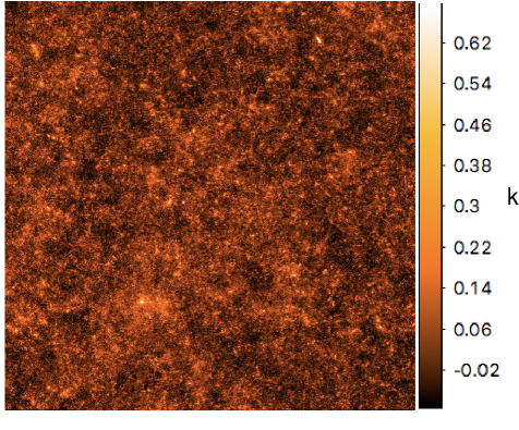
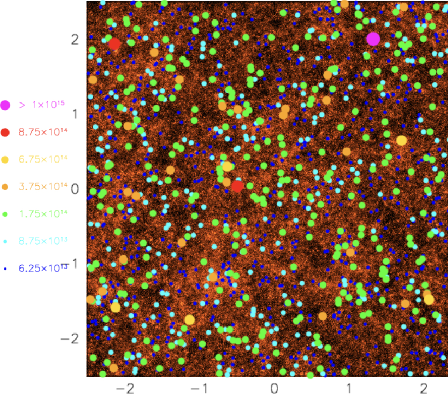
Figure 1: Left panel: convergence map ($5\times 5$ sq. degrees) of a light-cone realization up to $z_{s}=4$ constructed using the multi-plane ray-tracing glamer pipeline. Right panel: convergence map with over-plotted the haloes present within the light cone more massive than $5\times 10^{13}\mathrm{M_{\odot}}/h$. The various size coloured circles indicate haloes with different masses, as labelled in the plot. The masses refer to the FoF group definition.

Producing a large sample of realistic weak lensing simulations is becoming a challenging but necessary task for interpreting the outcomes of future wide field surveys. Importantly those allow ($1$) to mimic the survey geometry and masked regions ($2$) to consistently sample the expected weak lensing signals from the matter density distribution along the line of sight and ($3$) to construct reference models using the observed source redshift distribution from a given survey. A large number of light-cones plus weak lensing measurements is needed to ensure a good sampling of the non-linear properties of structure formation and to have under control the Gaussian and the non-Gaussian terms and the cosmic variance in estimating the covariance matrices (Harnois-Déraps et al., 2015a; Harnois-Déraps & van Waerbeke, 2015b).

In this paper, we use the halo model formalism for weak gravitational lensing, to quickly and accurately generate high-resolution convergence maps for any desired field of view and source redshift distribution in the context of a standard $\mathrm{\Lambda}$CDM cosmological scenario. Similarly (Li & Ostriker, 2002; Giocoli et al., 2012a; Giocoli et al., 2016) have used the lensing halo model formalism for strong lensing studies while (Kainulainen & Marra, 2011; Lin & Kilbinger, 2015a, b; Zorrilla Matilla et al., 2016) have used it for weak lensing predictions. The simulated maps can then be masked and cut to reproduce the geometry of the observed survey. The weak lensing statistical properties of the light-cones can also be sampled according to a realistic source sample, their redshift distribution and clustering. The extension of our method to a variety of non-standard cosmological models will be investigated in a forthcoming paper.

Our paper is organised as follows: in section 2 we present the reference numerical simulated light-cones with which we compare our model and describe the idea of the method, in section 3 we present our halo model for weak gravitational lensing and in section 4 we define the statistical estimators that we apply to our simulated light-cones to characterise their properties. In section 5, we summarise and discuss our results.

2 Model

In this work we present a fast method to produce weak lensing simulations using a halo model approach. In our analysis we use the halo catalogs corresponding to the particle light-cones extracted from a reference cosmological simulation. The light-cones have been produced by remapping the simulated snapshots into cuboids and projecting the particles into lens planes up to a given source redshift. In this work we will make use of the halo and subhalo catalogues to reconstruct the weak lensing field, using the halo model, in a desired field of view and compare it with the prediction obtained using the particles as tracers of the projected density. In this way, we statistically reconstruct the matter density distribution along the line-of-sight (Giocoli et al., 2015, 2016), avoiding replicating the same structures and producing gaps. The convergence maps have been computed from the projected lens planes using the ray-tracing glamer pipeline (Metcalf & Petkova, 2014) as described in Petkova et al. (2014).

2.1 The Numerical Simulation

In this section we present the reference numerical simulation we adopt and stress that our method is very general and ready to be applied to any halo – and subhalo – catalogue.

The cosmological parameters of our reference simulation have been set accordingly to the WMAP7 results. In particular, the numerical simulation used here is the $\mathrm{\Lambda}$CDM run extracted from the CoDECS suite (Baldi, 2012), where the initial conditions are generated using the N-GenIC code by displacing particles from a homogeneous ’glass’ distribution in order to set up a random-phase realisation of the linear matter power spectrum of the cosmological model according to Zel’dovich approximation (Zel’Dovich, 1970). The particles displacements are then rescaled to the desired amplitude of the density perturbation field at some high redshift ($z_{i}=99$), when all perturbation modes included in the simulation box are still evolving linearly. This redshift is then taken as the starting redshift of the simulation, and the corresponding particle distribution as the initial conditions for the N-body run. In setting the initial conditions for the simulation we have chosen $\Omega_{\rm CDM}=0.226$, $\Omega_{b}=0.0451$, $\Omega_{\Lambda}=0.729$, $h=0.703$ and $n_{s}=0.966$, the initial amplitude of the power spectrum at CMB time ($z_{\rm CMB}\approx 1100$) $A_{s}(z_{\rm CMB})=2.42\times 10^{-9}$ which correspond at $z=0$ to $\sigma_{8}=0.809$.

The simulation has a box size of $1$ comoving Gpc/$h$ aside and include $1024^{3}$ for both the components CDM and baryon for a total particle number of approximately $2\times 10^{9}$. The mass resolution is $m_{\rm CDM}=5.84\times 10^{10}\mathrm{M_{\odot}}/h$ for the cold dark matter component and $m_{b}=1.17\times 10^{10}\mathrm{M_{\odot}}/h$ for baryons, while the gravitational softening was set to $\epsilon_{g}=20\;\mathrm{kpc}/h$. Despite the presence of baryonic particles this simulation does not include hydrodynamics and is therefore a purely collisionless N-body run.

We stored about thirty snapshots between $z=10$ and $z=0$ at each simulation snapshot, halos have been identified using Friends-of-Friends (FoF) algorithm adopting a linking length parameter $b=0.2$ times the mean inter-particle separation of the CDM particles as primary tracers of the local mass density, and then attaching the baryonic particles to the FoF group of their nearest neighbours. Then, running subfind (Springel et al., 2001b) – on each simulation snapshot, for each FoF-group we compute $M_{\rm 200}$ as the mass enclosing a sphere with density $200$ times the critical density $\rho_{c}(z)$ at that redshift and assuming the particle with the minimum gravitational potential as the halo centre. subfind also searches for over-dense regions within a FoF group using a local SPH (Smoothed Particle Hydrodynamics) density estimate, identifying substructure candidates as regions bounded by an isodensity surface that crosses a saddle point of the density field. This algorithm is also testing that these possible substructures are physically bounded with an iterative unbinding procedure. In what follows, we will indicate with $M_{\rm FoF}$ the mass of the Friends-of-Friends group, with $M_{\rm 200}$ the mass of the sphere enclosing $200$ times the critical density of the universe and with $m_{\rm sub}$ the self-bound mass of substructures.

2.2 Building the past-light-cone with MapSim

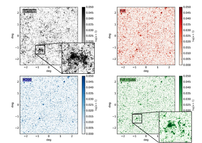
Figure 2: Convergence maps of a light-cone extending up to $z_{s}=4$. Top left panel: convergence maps created using ray-tracing in the light-cone constructed from the particles extracted from the simulation snapshots. Top right, bottom left and bottom right panels: convergence maps constructed using the halo model formalism based on $M_{\rm FoF}$, $M_{\rm 200}$ and $M_{\rm FoF}+m_{\rm sub}$ catalogs in the light-cone, respectively.

To build the lensing maps of the light-cone we piled together different slices of the simulation snapshots up to $z_{s}=4$. The size of the light-cone we consider has an angular aperture of $5$ deg, which combined with the comoving size of the simulation box of $1$ Gpc/$h$, ensures to uniformly construct the mass density distribution in redshift without gaps. For this purpose we use the MapSim code (Giocoli et al., 2015; Tessore et al., 2015) that extracts the particles from the simulation’s snapshot files and assembles them into a light-cone. The code initialises the memory and the grid size of the maps reading an input parameter file. This file contains information about the desired field of view (chosen to be $5$ deg on a side), the highest source redshift (in this case $z_{s}=4$) and the locations of the snapshot files. The number of required lens planes is decided ahead of time in order to avoid gaps in the constructed light-cones and the available stored simulation snapshots. We emphasize that in order to properly statistically sample the evolution of the matter density distribution as a function of the cosmic time within the light-cone we collapse in each lens plane the closest snapshot in redshift. The code, reading each snapshot file at a time from low to high redshift, extracts only the particle positions within the desired field of view and is not much memory consuming since it needs to allocate only a single snapshot file. The lens planes are built by mapping the particle positions to the nearest pre-determined plane, maintaining angular positions, and then pixelising the surface density using the triangular shaped cloud (TSC) method (Hockney & Eastwood, 1988). In constructing the lens planes we try to preserve as much as possibile the cosmological evolution of the structures by projecting into planes the snapshot with the closest redshift. The grid pixels are chosen to have the same angular size on all planes, equals to $2048\times 2048$, which allows to resolve approximately $8.8$ arcsec per pixel. The lens planes have been constructed each time a piece of simulation is taken from the stored particle snapshots; their number and recurrence depend on the number of snapshots stored while running the simulation. In particular in running our simulation we have stored $17$ snapshots from $z\sim 4$ to $z=0$ reasonably enough to construct a complete light-cone up to $z_{s}=4$ with $22$ lens planes. The selection and the randomisation of each snapshot is done as in Roncarelli et al. (2007) and discussed in more details in Giocoli et al. (2015). If the light-cone reaches the border of a simulation box before it reaches the redshift limit where the next snapshot will be used, the box is re-randomised and the light-cone extended through it again. Once the lens planes are created the lensing calculation itself is done using the glamer pipeline (Metcalf & Petkova, 2014; Petkova et al., 2014). Considering that at low redshifts, where many massive haloes are present, we have saved many snapshots – for example we use twelve snapshots up to redshift $z=1.2$ from which we produce fourteen lens planes – when projecting particles into separate lens planes we do not account for particle clumps in haloes that are located on the slice boundaries with particles on either side. As discussed by Hilbert et al. (2009) this effect can eventually produce an over-counting of particles that may bring a relative difference to the convergence power spectrum of approximately $0.1\%$.

Defining ${\boldsymbol{\theta}}$ the angular position on the sky and ${\boldsymbol{\beta}}$ the position on the source plane (the unlensed position), then a distortion matrix ${\bf A}$ can be defined as

$${\bf A}\equiv\frac{\partial{\boldsymbol{\beta}}}{\partial{\boldsymbol{\theta}}}=\left(\begin{array}[]{cc}1-\kappa-\gamma_{1}&\gamma_{2}\\ \gamma_{2}&1-\kappa+\gamma_{1}\end{array}\right)\,,$$ (3)

where $\kappa$ represents the convergence and the pseudo-vector ${\boldsymbol{\gamma}}\equiv\gamma_{1}+i\gamma_{2}$ the shear. In the case of a single lens plane, the convergence can be written as:

$$\kappa({\boldsymbol{\theta}})\equiv\frac{\Sigma({\boldsymbol{\theta}})}{\Sigma_{\rm crit}}\ ,$$ (4)

where $\Sigma({\boldsymbol{\theta}})$ represents the surface mass density and $\Sigma_{\rm crit}$ the critical surface density as:

$$\Sigma_{\rm crit}\equiv\dfrac{c^{2}}{4\pi G}\dfrac{D_{l}}{D_{s}D_{ls}},$$ (5)

where $c$ indicates the speed of light, $G$ the Newton’s constant and $D_{l}$, $D_{s}$ and $D_{ls}$ the angular diameter distances between observer-lens, observer-source and source-lens, respectively. In the case of multiple lens planes the situation is slightly different. After the deflection and shear maps on each plane are calculated, the light rays are traced from the observers through the lens planes up to the desired source redshift. The shear and convergence are also propagated through the planes as detailed in Petkova et al. (2014). glamer performs a complete ray-tracing calculation that takes into account non-linear coupling terms between the planes as well as correlations between the deflection and the shear. However, for this work when running the ray-tracing pipeline we have adopted the Born approximation, that is following the light-rays along unperturbed paths. As discussed in Giocoli et al. (2016) – by performing a full ray-tracing comparison – and in Schäfer et al. (2012) – by computing an analytic perturbative expansion – the Born approximation is an excellent approximation for weak cosmic lensing down to very small scales ($l\geq 10^{4}$). We underline that the physical modelling at these very small scales is far from the purpose of this work and we are aware that it may eventually need a correct and self-consistent treatment of the baryonic components (Mohammed et al., 2014; Harnois-Déraps et al., 2015a).

In the left panel of Fig. 1 we show the convergence map of the first light-cone realisation assuming a source redshift $z_{s}=4$. In order to have various statistical samples, we have created $25$ light-cone realisations. They can be treated as independent since do not contain the same structures along the line-of-sight, considering the size of the simulation box $1$Gpc/$h$ and the field of view of $5$ deg on a side.

Within the MapSim code we have recently implemented also the possibility to construct a corresponding light-cone of haloes and subhaloes that resemble the underlying randomisation of the associated matter density distribution along the line-of-sight. Friends-of-Friends groups, $M_{\rm 200}$-haloes and subhaloes are subdivided according to the various constructed planes; for each of them we compute the corresponding redshift from their comoving distance from the observer and their angular position in the sky with respect to the assumed field of view. In order to avoid edge effects when re-constructing the lensing properties from virialized structures, we extracted haloes and subhaloes from a field of view $2.5$ deg larger on each side. This means that haloes and subhaloes are extracted from a region of $10\times 10$ sq. degrees, centered in the same sky position as the cone from which we extract the particles. Halo and subhalo catalogues are saved in complementary files with respect to the corresponding lens planes. We highlight that in order not to double-count the mass in haloes we do not consider the main subhalo within the subfind catalogues which typically account for the smooth halo component. As an example in the right panel of Fig. 1 we plot on top the convergence map, the positions of the FoF groups more massive than $5\times 10^{13}\mathrm{M_{\odot}}/h$ within the light-cone from $z=0$ to $z_{s}=4$. The various size coloured circles refer to different masses as indicated in the label.

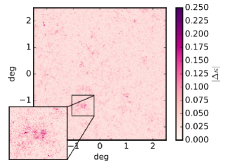
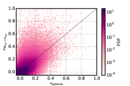
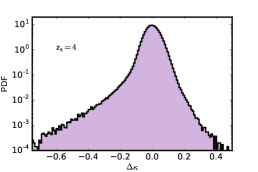
Figure 3: Left panel: absolute difference between the convergence map computed using particles and the one using FoF-haloes plus subhaloes. Central panel: pixel by pixel correlation between the two maps. Right panel: probability distribution function of the difference between the two maps.

3 A Weak Lensing Halo Model approach: WL-MOKA

The different statistical analyses performed in the last twenty-years on the post-processing data of various numerical simulations have given the possibility to reconstruct in good details the dark matter halo structural properties over a wide range of masses (Springel et al., 2001b; Gao et al., 2004; Giocoli et al., 2008). In particular, many works seem to converge toward the idea that virialized haloes tend to possess a well defined density profile (Navarro et al., 1996; Moore et al., 1998; Rasia et al., 2004). Following the Navarro et al. (1996) (hereafter NFW) prescription we assume the density profile of haloes to follow the relation:

$$\rho(r|M_{\rm h})=\frac{\rho_{s}}{(r/r_{s})(1+r/r_{s})^{2}}\,,$$ (6)

where $r_{s}$ is the scale radius, defining the concentration $c_{\rm h}\equiv R_{\rm h}/r_{s}$ and $\rho_{s}$ the dark matter density at the scale radius:

$$\rho_{s}=\frac{M_{\rm h}}{4\pi r_{s}^{3}}\left[\ln(1+c_{\rm h})-\frac{c_{\rm h}}{1+c_{\rm h}}\right]^{-1}\,,$$ (7)

$R_{\rm h}$ is the radius of the halo which may varies depending on the halo over-density definition. In this analysis we will adopt ($i$) the mass inside the Virial radius for the FoF groups:

$$M_{\rm vir}=\frac{4\pi}{3}R_{\rm vir}^{3}\frac{\Delta_{\rm vir}}{\Omega_{m}(z)}\Omega_{0}\rho_{c}\,,$$ (8)

and ($ii$) the mass inside a sphere enclosing $200$ times the critical matter density $\rho_{c}(z)$ of the Universe:

$$M_{\rm 200}=\frac{4\pi}{3}R_{\rm 200}^{3}200\frac{\Omega_{0}}{\Omega_{\rm m}(z)}\rho_{c}\,,$$ (9)

where $\Omega_{0}\equiv\Omega_{\rm m}(0)$ represents the matter density parameter at the present time and $\Delta_{\rm vir}$ is the virial over-density (Eke et al., 1996; Bryan & Norman, 1998), $R_{\rm vir}$ and $R_{\rm 200}$ symbolise the virial and the $200$ critical radius of the halo, that is the distance from the halo centre that encloses the desired density contrast; $\rho_{c}$ represents the critical density at the present time.

The halo concentration $c_{\rm h}$ is a decreasing function of the host halo mass. This relation is explained in terms of hierarchical clustering within CDM-universes and of different halo-formation histories (van den Bosch, 2002; De Boni et al., 2016). Small haloes form first in a denser universe and then merge together forming the more massive ones: galaxy clusters sit at the peak of the hierarchical pyramid being the more recent structures to form (Bond et al., 1991; Lacey & Cole, 1993; Sheth & Tormen, 2004a; Giocoli et al., 2007). This trend is reflected in the mass-concentration relation: at a given redshift smaller haloes are more concentrated than larger ones. Different fitting functions for numerical mass-concentration relations have been presented by various authors (Bullock et al., 2001; Neto et al., 2007; Duffy et al., 2008; Gao et al., 2008). In this work, we adopt the relation proposed by Zhao et al. (2009) which links the concentration of a given halo with the time $t_{0.04}$ at which its main progenitor assembles $4$ percent of its mass. Giocoli et al. (2012b) have found that this relation works very well for virialized masses $M_{\rm vir}$ while the parameters of the model need to be slightly modified for the $M_{\rm 200}$ definition (Giocoli et al., 2013). We want to underline that the model by Zhao et al. (2009) also fits numerical simulations with different cosmologies; it seems to be of reasonably general validity within few percents of accuracy. For the mass accretion history model of the two mass over-density definitions ($M_{\rm vir}$ or $M_{\rm 200}$) we adopt the relations by Giocoli et al. (2012b) and Giocoli et al. (2013). Those models are quite universals and give the possibility to generalise the relations eventually also to non-standard models (Giocoli et al., 2013). In particular, the concentration mass relation mainly impacts on the behaviour of the power spectrum at scales below $1\,h^{-1}$Mpc as discussed in details by Giocoli et al. (2010).

Due to different assembly histories, haloes with same mass at the same redshift may have different concentrations (Navarro et al., 1996; Jing, 2000; Wechsler et al., 2002; Zhao et al., 2003a, b). At fixed host halo mass, the distribution in concentration is well described by a lognormal distribution function with a rms $\sigma_{\ln c}$ between $0.1$ and $0.25$ (Jing, 2000; Dolag et al., 2004; Sheth & Tormen, 2004b; Neto et al., 2007). In this work we adopt a lognormal distribution with $\sigma_{\ln c}=0.25$.

In our numerical simulation, subhaloes have been identified using the subfind algorithm. For the mass density distribution in subhaloes we adopt the truncated Singular Isothermal Sphere (hereafter tSIS) profile. This model accounts for the fact that the subhalo density profiles are modified by tidal stripping due to close interactions with the main halo smooth component and to close encounters with other clumps, gravitational heating, and dynamical friction. Such events can cause the subhaloes to lose mass, and may eventually result in their complete disruption (Hayashi et al., 2003; Choi et al., 2007). We model the dark matter density profile in subhaloes as (Keeton, 2003),

$$\rho_{\rm sub}(r)=\left\{\begin{array}[]{ll}\dfrac{\sigma_{v}^{2}}{2\pi Gr^{2}}&r\leq R_{sub},\\ 0&r>R_{sub}\\ \end{array}\right.$$ (10)

with velocity dispersion $\sigma_{v}$, and $R_{sub}$ defined as:

$$m_{sub} = \int_{0}^{R_{sub}}4\pi r^{2}\rho_{sub}(r)\mathrm{d}r\Rightarrow$$

$$R_{sub} = \dfrac{G\,m_{sub}}{2\,\sigma_{v}^{2}}\,.$$ (11)

To compute the velocity dispersion we use the same implementation described in the MOKA code by Giocoli et al. (2012a). The tSIS profile well represents galaxy density profiles on scales relevant for strong lensing. Previously, different authors have used this model to characterise the lensing signal by substructures after stripping (Metcalf & Madau, 2001).
In Table 1 we summarise the halo model properties which we use to construct the convergence maps using our algorithm.

Table 1: Summary of the halo and subhalo properties considered in our models when building the effective convergence maps

Case	c-M relation	profile
FoF	Zhao et al. (2009)	NFW
M200	Giocoli et al. (2013)	NFW
FoF+Subs	Zhao et al. (2009)	NFW (haloes)+ tSIS (subhaloes)

Assuming spherical symmetry for the matter density profile in haloes, we can compute the surface mass density $\Sigma(x_{1},x_{2})$ associated with a density profile $\rho(r)$ extending up to the virial radius $R_{\rm vir}$ as:

$$\Sigma(x_{1},x_{2})=2\int_{0}^{R_{\rm vir}}\rho(x_{1},x_{2},\zeta)\mathrm{d}\zeta,$$ (12)

where $x_{1}$, $x_{2}$ and $\zeta$ represents the three-dimensional coordinates and $r^{2}=x_{1}^{2}+y_{2}^{2}+\zeta^{2}$; this quantity is then used to define the convergence as in eq. (4).

As described by Bartelmann (1996) the Navarro-Frank-White density profile has a well defined primitive for the integral in equation (12) and its convergence can be derived analytically, as well as for the tSIS profile.

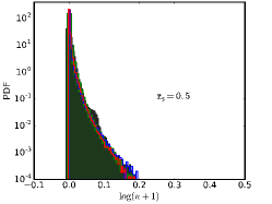
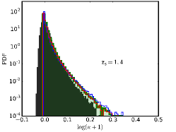
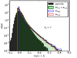
Figure 4: Probability Distribution Functions (PDF) of the convergence maps presented in Fig. 2. Left, central and right panels show the PDFs for three different source redshifts: $z_{s}=0.5$, $1.4$ and $4$, respectively. The black histograms show the PDF for the convergence map constructed using the glamer ray-tracing pipeline, while the blue and red are the ones computed from the $M_{\rm 200}$ and $M_{\rm FoF}$ halo catalogues. The green histograms show the distribution function of the convergence map where the Friends-of-Friends haloes contain also substructures.

In Fig. 2, we show 4 convergence maps of the same light-cone realisation extending up to redshift $z_{s}=4$. In the top left panel (in black scale), we created the convergence map using ray-tracing in the light-cone constructed from the particles extracted from the simulation snapshots. In the top right (in red scale) and bottom left (in blue scale) we present the convergence maps constructed using the $M_{\rm FoF}$ and the $M_{\rm 200}$ halo catalogues, respectively. By eye it is possible to spot that using the halo catalogues the overall surface mass density distribution is quite well traced. However it is noticeable with more careful analysis that the map constructed using the Friends-of-Friends catalogue presents much more clustering of low mass haloes. This is be due ($i$) to numerical resolution of the simulation: FoF haloes with less than 10 particles within $200$ times the critical density are not well resolved and not stored in the corresponding $M_{\rm 200}$ catalogue and ($ii$) to the possible non universality of the mass function defined with $M_{\rm 200}$ haloes (Tinker et al., 2008; Despali et al., 2016). In general it is interesting to notice that $M_{\rm FoF}$ and $M_{\rm 200}$ contain typically a different fraction of the total mass in the simulation. Using the relations calibrated from numerical simulations by Despali et al. (2016), we notice assuming the same mass resolution – down to ten dark matter particles – and box-size of our reference run, at $z=0$. The mass contained in $M_{\rm FoF}$ haloes is approximately $30\%$ of the total mass in the simulation, while in $M_{\rm 200}$ haloes it is less than $25\%$; at $z=1$ the two fractions become $15\%$ and $12\%$, respectively, while at $z=3$ they are both approximately $1.5\%$, since the two mass over-density definitions get closer and closer at high redshifts (Eke et al., 1996; Bryan & Norman, 1998).

Convergence maps constructed by summing the surface mass density contribution of all haloes present within the halo catalogues, and weighting them with the critical surface density as in eq. (4), are effective convergence maps and are forced to have an average value of the convergence $\bar{\kappa}=\dfrac{\sum_{i=1}^{N_{pix}}\kappa_{i}}{N_{pix}}=0$. This implies that conservatively each convergence map describes the perturbed matter density distribution with respect to an average background value. We underline also that this point is important when we construct the effective convergence maps using only haloes or using both haloes and subhaloes; in order not to over-count the masses in both cases the average value of the convergence in each constructed plane is set to be zero. This kind of approach has also been used in constructing the convergence map implying the full ray-tracing technique – as in the top left panel of the figure: since the rays are propagated between planes using the standard distances in a Robertson-Walker metric which assumes a uniform distribution of matter the addition of matter on each of the planes will, in a sense, over-count the mass in the universe. Without correcting for this, the average convergence from the planes will be positive and will cause the average distance for a fixed redshift to be smaller than it should be. To compensate for the contained density between the planes, the ensemble average density on each plane is subtracted. Each plane then has zero convergence on average and the average redshift-distance relation is as it would be in a perfectly homogeneous universe. Finally, the bottom right panel of Fig. 2 (in green scale) presents the convergence map constructed using the FoF haloes plus the subhaloes. In this case comparing this map with respect to the one in red scale, where we use only the FoF haloes, we notice an increase of small scale perturbations. In Fig. 3 we display the statistical difference between the maps computed using particles and FoF-haloes plus subhaloes. In the left panel we show the absolute difference map between the two cases. The central panel exhibits the pixel by pixel correlation between the two maps, while the left panel presents the Probability Distribution Function (PDF) of the difference $\Delta\kappa=\kappa_{\rm particles}-\kappa_{\rm M_{FoF}+m_{sub}}$. From the figures what is mainly appearing is that the effective convergence map computed using haloes and subhaloes mainly trace the matter density distribution on small scales where non-linear structures and clumps are present, however still differences appear mainly due to projection effects, filamentary structures – as better displayed in the small panel in the left figure – and sheets.

3.1 Probability Distribution Function of the Convergence Fields

To quantify the previous discussion, in Fig. 4 we display the Probability Distribution Function of the convergence maps presented in Fig. 2. Left, central and right panels show the PDF of the convergence constructed for sources at $z_{s}=0.5$, $1.4$ and $4$, respectively. Black, red, blue and green coloured histograms show the four corresponding cases used to construct the convergence map: particles, FoF groups, $M_{\rm 200}$-haloes, and FoF groups with subhaloes. From the panels in the figure, we notice that for $z_{s}=0.5$ the four histograms are very similar and that the inclusion of substructures creates some pixels with larger convergence values which may correspond to the core of clumps. In the central and right panels we notice that the PDF of the convergence map constructed using the particles does not present pixels with convergence $\kappa\gtrsim 0.75$, this is probably due to the numerical and force resolution of the simulation which does not permit to resolve with a reasonable number of particles the cores of haloes and subhaloes. In addition, the black histograms display distinct tails with negative convergence. This is probably due to the sampling of the matter density distribution that is not bound to haloes – and that we are missing in our halo modelling formalism. We will discuss more about that in the next sections.

3.2 Building up the convergence power spectra

Following the halo model formalism, the matter density distribution in the universe is assumed to be associated to virialized haloes (Cooray & Sheth, 2002). The mean density within the Universe can so be computed from the relation:

$$\bar{\rho}=\int m\;n(m)\;\mathrm{d}m,$$ (13)

where $n(m)$ represents the halo mass function. The three-dimensional matter power spectrum can be then decomposed in:

$$P_{\rm\delta}(k,z)=P_{\rm 1h}(k,z)+P_{\rm 2h}(k,z),$$ (14)

where $P_{\rm 1h}(k)$ represents the power spectrum of the matter density distribution within one halo, while $P_{\rm 2h}(k)$ describes the power spectrum of the matter density distribution between two distant haloes. The two terms can be read as:

$$P_{\rm 1h}(k,z)= \int\left(\dfrac{m}{\bar{\rho}}\right)^{2}n(m,z)u^{2}(k|m)\mathrm{d}m$$ (15)

$$P_{\rm 2h}(k,z)= \int\left(\dfrac{m_{1}}{\bar{\rho}}\right)n(m_{1},z)u(k|m_{1})\mathrm{d}m_{1}$$

$$\int\left(\dfrac{m_{2}}{\bar{\rho}}\right)n(m_{2},z)u(k|m_{2})\mathrm{d}m_{2}P_{\rm hh}(k|m_{1},m_{2}),$$

where $u(k|m)$ represents the Fourier transform of the dark matter density profile and $P_{\rm hh}(k|m_{1},m_{2})$ describes the halo-halo power spectrum that can be expressed in terms of the halo-matter bias parameter $b(m)$ and the linear matter power spectrum $P_{\delta,\rm lin}(k)$:

$$P_{\rm hh}(k|m_{1},m_{2})=b(m_{1})b(m_{2})P_{\delta,\rm lin}(k).$$ (17)

Including the presence of substructures within haloes adds more equations to the halo model that can be trivially solved considering the correlation between the smooth and the clump components both within the 1-halo and the 2-halo term (Sheth & Jain, 2003; Giocoli et al., 2010).

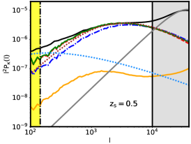
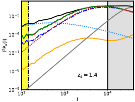
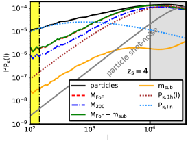
Figure 5: Convergence power spectra averaged over $25$ different realisations of the light-cones considering sources at three fixed source redshifts, from left to right we have $z_{s}=0.5$, $z_{s}=1.4$ and $z_{s}=4$. The black curves show the power spectra computed from the ray-tracing pipeline including all the particles in the light-cone extracted from the numerical simulation (as described in Giocoli et al. (2015)). The red dashed and blue dot-dashed curves show the results of the two considered halo catalogues $M_{\rm FoF}$ and $M_{\rm 200}$, while the solid orange lines present the contribution of the substructures. The solid green curves display the total convergence power spectra of Friends-of-Friends haloes and subhaloes. The grey curves describe the shot-noise contribution to the power spectra computed from the ray-tracing simulations using particles.

The convergence power spectrum, to first order, can be expressed as an integral of the three-dimensional matter power spectrum computed from the observer looking at the past lightcone from the present epoch up to a given source redshift (Bartelmann & Schneider, 2001). In this approximation it is assumed that the light rays travel along unperturbed paths and all terms higher than first order in convergence and shear can be ignored. Defining $f(w)$ as the angular radial function, that depends on the comoving radial coordinate $w$ given the curvature of the universe, we can write the convergence power spectrum at a given source redshift $z_{s}$ – with a corresponding radial coordinate $w_{s}$ – as:

$$P_{\kappa}(l)=\dfrac{9H_{0}^{4}\Omega_{m}^{2}}{4c^{4}}\int_{0}^{w_{s}(z_{s})}\dfrac{f^{2}(w_{s}-w)}{f^{2}(w_{s})a^{2}(w)}P_{\rm\delta}\left(\dfrac{l}{f(w)},w\right)\,\mathrm{d}w.$$ (18)

Analogously from the constructed effective convergence maps we can compute the corresponding power spectrum as:

$$\langle\hat{\kappa}(\mathbf{l})\hat{k^{*}}(\mathbf{l}^{\prime})\rangle={4\pi^{2}}\delta_{D}(\mathbf{l}-\mathbf{l}^{\prime})P_{\kappa}(l),$$ (19)

where $\delta_{D}^{(2)}$ represents the Delta Dirac in two dimensions.

In Fig. 5 we present the average power spectrum of $25$ different light-cone realisations for three different source redshifts: $z_{s}=0.5$, $z_{s}=1.4$ and $z_{s}=4$, from left to right respectively. In each panel, the black curves display the spectra computed using the ray-tracing pipeline on the particle distribution and the grey curves show the associated particle shot-noise (Vale & White, 2003; Giocoli et al., 2016). The shaded grey area marks the region where the shot-noise term of the particles starts to dominate the cosmic shear measurements, while the yellow shaded region indicates the part below the angular Nyqvist mode sampled by our field of view. Red dashed and blue dot-dashed curves show the power spectra computed using the FoF and the $M_{\rm 200}$ haloes present within the light-cones. The orange curves describe the contribution of the subhaloes while the green solid curves exhibit the total contribution of the Friends-of-Friends haloes and their associated subhaloes. From the figure we can observe that the large scale behaviour of our halo model power spectra manifests less power than expected from linear theory (dotted light-blue curves). The magenta dashed curves display the one-halo term contribution of the analytical halo model as in eq. (15) where we have integrated the theoretical mass function (Sheth & Tormen, 1999) from the minimum halo mass that we have in the simulation $M_{\rm min}\approx 2.07\times 10^{12}M_{\odot}/h$ for consistency. From the figure we notice that our halo model for weak lensing captures quite well the 1-halo term plus the one related to the matter between haloes, but misses the linear contribution of matter distributed among haloes; that is matter density fluctuations that are not attached to non-linear structures, and possibly tracing sheets and filaments.

The relative contribution of subhaloes to the power spectrum with respect to the smooth component is displayed in Fig. 6. The green, blue and red curves represent the subhalo contribution for three different source redshifts. From the figure, we notice that typically subhaloes contribute to approximately $3\%$ to the convergence power spectrum and that their contribution becomes significant for scales below $5$ arcmin, which correspond to approximately is $l\approx 10^{4}$. In particular those scales are not well resolved within the numerical simulation due to particle and force limitations while well described by our halo model formalism. We remind the reader that in those regimes, a consistent treatment of the baryonic contribution is very critical (Harnois-Déraps et al., 2015a), and this will be addressed in an upcoming paper (Giocoli, Monaco et al. in preparation).

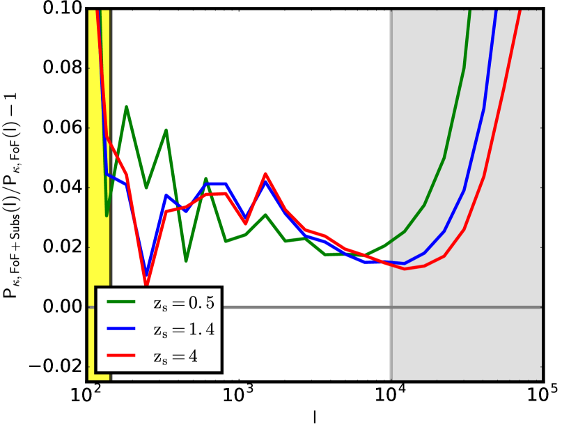
Figure 6: Relative contribution to the cosmic shear power spectrum of the subhaloes with respect to the FoF-haloes for three different source redshifts: $z_{s}=0.5$ (green), $z_{s}=1.4$ (blue) and $z_{s}=4$ (red).

3.3 Effective linear contribution to the weak lensing halo model

As discussed in the previous section, the halo model formalism we have implemented so far is missing the effective contribution of the linear matter density distribution presents among the haloes, which may be tracing sheets and filaments. Recently van Daalen & Schaye (2015), using a set of cosmological numerical simulations, discussed how much non-virialized matter contributes to the total matter power spectrum. In particular they showed that the larger the region around the virialized haloes that is included, the larger the halo contribution to the matter power spectrum will be. The matter power spectrum of haloes for $3<k<100\,h\mathrm{Mpc^{-1}}$ enclosing $200$ times the critical density is smaller then that enclosing $200$ times the background and, in turn, of that of the mass residing within the FoF groups. Going from three to two dimensions it can be noticed from the panels present in Fig. 5, our model properly reconstructs the 1-halo term plus a 2-halo-like term but has less power at large scales with respect to the ray-tracing power spectrum as computed using particles. Consistent with the results of van Daalen & Schaye (2015), we notice that the convergence power spectra of the matter in $M_{\rm 200}$ is smaller than that of the matter within the FoF groups. However the relative difference between the two depends on the considered source redshift: $M_{\rm 200}$ has a pseudo-redshift evolution, as discussed by Diemer et al. (2013), that depends on the evolution of the Hubble function with the cosmic time. To better clarify and understand the contribution of the matter in virialized haloes, in Fig. 7 we display the convergence power spectrum for sources at redshift $z_{s}=4$. The black curve represents the power spectrum from the ray-tracing simulation using particles for one light-cone realisation, while the green curve displays our halo model contribution from haloes and subhaloes. The cyan dotted line shows the convergence power spectrum $P_{\kappa,\rm lin}(l)$ computed from the linear theory assuming $z_{s}=4$, while the blue curve displays the power spectrum of a random Gaussian realisation $\kappa_{\rm lin,r}$ of the theoretical linear cosmic shear power spectrum $P_{\kappa,\rm lin}(l)$ in amplitude with a random phase – the subscript r stands for random in phase. The dashed orange curve – almost overlapping the red one – presents the convergence power spectrum of a map computed by summing our halo model convergence map $\kappa_{\rm hm}$ – halo and subhalo contribution – with $\kappa_{\rm lin,r}$ calculated for $z_{s}=4$. Computing its power spectrum, because the cross-terms are zero, we can read:

$$\langle\hat{\kappa}(\mathbf{l})\hat{k^{*}}(\mathbf{l}^{\prime})\rangle = \langle\begin{array}[]{c}\mathchoice{\raisebox{-1.07745pt}{\leavevmode\resizebox{485.1532pt}{2.15277pt}{\hbox{\raisebox{506.89pt}{$\displaystyle\mathchoice{\raisebox{0.0pt}{\leavevmode\resizebox{179.31073pt}{505.89pt}{\hbox{\raisebox{0.0pt}{$\displaystyle\mathchoice{\raisebox{0.0pt}{\leavevmode\resizebox{44.82768pt}{505.89pt}{\hbox{\raisebox{2.0pt}{$\displaystyle\kern-0.5pt\bigwedge\kern-0.5pt$}}}}}{\raisebox{0.0pt}{\leavevmode\resizebox{44.82768pt}{505.89pt}{\hbox{\raisebox{2.0pt}{$\textstyle\kern-0.5pt\bigwedge\kern-0.5pt$}}}}}{\raisebox{0.0pt}{\leavevmode\resizebox{44.82768pt}{505.89pt}{\hbox{\raisebox{1.4pt}{$\scriptstyle\kern-0.5pt\bigwedge\kern-0.5pt$}}}}}{\raisebox{0.0pt}{\leavevmode\resizebox{44.82768pt}{505.89pt}{\hbox{\raisebox{1.0pt}{$\scriptscriptstyle\kern-0.5pt\bigwedge\kern-0.5pt$}}}}}$}}}}}{\raisebox{0.0pt}{\leavevmode\resizebox{179.31073pt}{505.89pt}{\hbox{\raisebox{0.0pt}{$\textstyle\mathchoice{\raisebox{0.0pt}{\leavevmode\resizebox{44.82768pt}{505.89pt}{\hbox{\raisebox{2.0pt}{$\displaystyle\kern-0.5pt\bigwedge\kern-0.5pt$}}}}}{\raisebox{0.0pt}{\leavevmode\resizebox{44.82768pt}{505.89pt}{\hbox{\raisebox{2.0pt}{$\textstyle\kern-0.5pt\bigwedge\kern-0.5pt$}}}}}{\raisebox{0.0pt}{\leavevmode\resizebox{44.82768pt}{505.89pt}{\hbox{\raisebox{1.4pt}{$\scriptstyle\kern-0.5pt\bigwedge\kern-0.5pt$}}}}}{\raisebox{0.0pt}{\leavevmode\resizebox{44.82768pt}{505.89pt}{\hbox{\raisebox{1.0pt}{$\scriptscriptstyle\kern-0.5pt\bigwedge\kern-0.5pt$}}}}}$}}}}}{\raisebox{0.0pt}{\leavevmode\resizebox{126.53174pt}{505.89pt}{\hbox{\raisebox{0.0pt}{$\scriptstyle\mathchoice{\raisebox{0.0pt}{\leavevmode\resizebox{31.63293pt}{505.89pt}{\hbox{\raisebox{1.4pt}{$\displaystyle\kern-0.5pt\bigwedge\kern-0.5pt$}}}}}{\raisebox{0.0pt}{\leavevmode\resizebox{31.63293pt}{505.89pt}{\hbox{\raisebox{1.4pt}{$\textstyle\kern-0.5pt\bigwedge\kern-0.5pt$}}}}}{\raisebox{0.0pt}{\leavevmode\resizebox{31.63293pt}{505.89pt}{\hbox{\raisebox{0.98pt}{$\scriptstyle\kern-0.5pt\bigwedge\kern-0.5pt$}}}}}{\raisebox{0.0pt}{\leavevmode\resizebox{31.63293pt}{505.89pt}{\hbox{\raisebox{0.7pt}{$\scriptscriptstyle\kern-0.5pt\bigwedge\kern-0.5pt$}}}}}$}}}}}{\raisebox{0.0pt}{\leavevmode\resizebox{104.86858pt}{505.89pt}{\hbox{\raisebox{0.0pt}{$\scriptscriptstyle\mathchoice{\raisebox{0.0pt}{\leavevmode\resizebox{26.21715pt}{505.89pt}{\hbox{\raisebox{1.0pt}{$\displaystyle\kern-0.5pt\bigwedge\kern-0.5pt$}}}}}{\raisebox{0.0pt}{\leavevmode\resizebox{26.21715pt}{505.89pt}{\hbox{\raisebox{1.0pt}{$\textstyle\kern-0.5pt\bigwedge\kern-0.5pt$}}}}}{\raisebox{0.0pt}{\leavevmode\resizebox{26.21715pt}{505.89pt}{\hbox{\raisebox{0.7pt}{$\scriptstyle\kern-0.5pt\bigwedge\kern-0.5pt$}}}}}{\raisebox{0.0pt}{\leavevmode\resizebox{26.21715pt}{505.89pt}{\hbox{\raisebox{0.5pt}{$\scriptscriptstyle\kern-0.5pt\bigwedge\kern-0.5pt$}}}}}$}}}}}$}}}}}{\raisebox{-1.07745pt}{\leavevmode\resizebox{485.1532pt}{2.15277pt}{\hbox{\raisebox{506.89pt}{$\textstyle\mathchoice{\raisebox{0.0pt}{\leavevmode\resizebox{179.31073pt}{505.89pt}{\hbox{\raisebox{0.0pt}{$\displaystyle\mathchoice{\raisebox{0.0pt}{\leavevmode\resizebox{44.82768pt}{505.89pt}{\hbox{\raisebox{2.0pt}{$\displaystyle\kern-0.5pt\bigwedge\kern-0.5pt$}}}}}{\raisebox{0.0pt}{\leavevmode\resizebox{44.82768pt}{505.89pt}{\hbox{\raisebox{2.0pt}{$\textstyle\kern-0.5pt\bigwedge\kern-0.5pt$}}}}}{\raisebox{0.0pt}{\leavevmode\resizebox{44.82768pt}{505.89pt}{\hbox{\raisebox{1.4pt}{$\scriptstyle\kern-0.5pt\bigwedge\kern-0.5pt$}}}}}{\raisebox{0.0pt}{\leavevmode\resizebox{44.82768pt}{505.89pt}{\hbox{\raisebox{1.0pt}{$\scriptscriptstyle\kern-0.5pt\bigwedge\kern-0.5pt$}}}}}$}}}}}{\raisebox{0.0pt}{\leavevmode\resizebox{179.31073pt}{505.89pt}{\hbox{\raisebox{0.0pt}{$\textstyle\mathchoice{\raisebox{0.0pt}{\leavevmode\resizebox{44.82768pt}{505.89pt}{\hbox{\raisebox{2.0pt}{$\displaystyle\kern-0.5pt\bigwedge\kern-0.5pt$}}}}}{\raisebox{0.0pt}{\leavevmode\resizebox{44.82768pt}{505.89pt}{\hbox{\raisebox{2.0pt}{$\textstyle\kern-0.5pt\bigwedge\kern-0.5pt$}}}}}{\raisebox{0.0pt}{\leavevmode\resizebox{44.82768pt}{505.89pt}{\hbox{\raisebox{1.4pt}{$\scriptstyle\kern-0.5pt\bigwedge\kern-0.5pt$}}}}}{\raisebox{0.0pt}{\leavevmode\resizebox{44.82768pt}{505.89pt}{\hbox{\raisebox{1.0pt}{$\scriptscriptstyle\kern-0.5pt\bigwedge\kern-0.5pt$}}}}}$}}}}}{\raisebox{0.0pt}{\leavevmode\resizebox{126.53174pt}{505.89pt}{\hbox{\raisebox{0.0pt}{$\scriptstyle\mathchoice{\raisebox{0.0pt}{\leavevmode\resizebox{31.63293pt}{505.89pt}{\hbox{\raisebox{1.4pt}{$\displaystyle\kern-0.5pt\bigwedge\kern-0.5pt$}}}}}{\raisebox{0.0pt}{\leavevmode\resizebox{31.63293pt}{505.89pt}{\hbox{\raisebox{1.4pt}{$\textstyle\kern-0.5pt\bigwedge\kern-0.5pt$}}}}}{\raisebox{0.0pt}{\leavevmode\resizebox{31.63293pt}{505.89pt}{\hbox{\raisebox{0.98pt}{$\scriptstyle\kern-0.5pt\bigwedge\kern-0.5pt$}}}}}{\raisebox{0.0pt}{\leavevmode\resizebox{31.63293pt}{505.89pt}{\hbox{\raisebox{0.7pt}{$\scriptscriptstyle\kern-0.5pt\bigwedge\kern-0.5pt$}}}}}$}}}}}{\raisebox{0.0pt}{\leavevmode\resizebox{104.86858pt}{505.89pt}{\hbox{\raisebox{0.0pt}{$\scriptscriptstyle\mathchoice{\raisebox{0.0pt}{\leavevmode\resizebox{26.21715pt}{505.89pt}{\hbox{\raisebox{1.0pt}{$\displaystyle\kern-0.5pt\bigwedge\kern-0.5pt$}}}}}{\raisebox{0.0pt}{\leavevmode\resizebox{26.21715pt}{505.89pt}{\hbox{\raisebox{1.0pt}{$\textstyle\kern-0.5pt\bigwedge\kern-0.5pt$}}}}}{\raisebox{0.0pt}{\leavevmode\resizebox{26.21715pt}{505.89pt}{\hbox{\raisebox{0.7pt}{$\scriptstyle\kern-0.5pt\bigwedge\kern-0.5pt$}}}}}{\raisebox{0.0pt}{\leavevmode\resizebox{26.21715pt}{505.89pt}{\hbox{\raisebox{0.5pt}{$\scriptscriptstyle\kern-0.5pt\bigwedge\kern-0.5pt$}}}}}$}}}}}$}}}}}{\raisebox{0.0pt}{\leavevmode\resizebox{413.01508pt}{2.15277pt}{\hbox{\raisebox{0.0pt}{$\scriptstyle\mathchoice{\raisebox{0.0pt}{\leavevmode\resizebox{125.51758pt}{505.89pt}{\hbox{\raisebox{0.0pt}{$\displaystyle\mathchoice{\raisebox{0.0pt}{\leavevmode\resizebox{31.3794pt}{505.89pt}{\hbox{\raisebox{1.4pt}{$\displaystyle\kern-0.5pt\bigwedge\kern-0.5pt$}}}}}{\raisebox{0.0pt}{\leavevmode\resizebox{31.3794pt}{505.89pt}{\hbox{\raisebox{1.4pt}{$\textstyle\kern-0.5pt\bigwedge\kern-0.5pt$}}}}}{\raisebox{0.0pt}{\leavevmode\resizebox{31.3794pt}{505.89pt}{\hbox{\raisebox{0.98pt}{$\scriptstyle\kern-0.5pt\bigwedge\kern-0.5pt$}}}}}{\raisebox{0.0pt}{\leavevmode\resizebox{31.3794pt}{505.89pt}{\hbox{\raisebox{0.7pt}{$\scriptscriptstyle\kern-0.5pt\bigwedge\kern-0.5pt$}}}}}$}}}}}{\raisebox{0.0pt}{\leavevmode\resizebox{125.51758pt}{505.89pt}{\hbox{\raisebox{0.0pt}{$\textstyle\mathchoice{\raisebox{0.0pt}{\leavevmode\resizebox{31.3794pt}{505.89pt}{\hbox{\raisebox{1.4pt}{$\displaystyle\kern-0.5pt\bigwedge\kern-0.5pt$}}}}}{\raisebox{0.0pt}{\leavevmode\resizebox{31.3794pt}{505.89pt}{\hbox{\raisebox{1.4pt}{$\textstyle\kern-0.5pt\bigwedge\kern-0.5pt$}}}}}{\raisebox{0.0pt}{\leavevmode\resizebox{31.3794pt}{505.89pt}{\hbox{\raisebox{0.98pt}{$\scriptstyle\kern-0.5pt\bigwedge\kern-0.5pt$}}}}}{\raisebox{0.0pt}{\leavevmode\resizebox{31.3794pt}{505.89pt}{\hbox{\raisebox{0.7pt}{$\scriptscriptstyle\kern-0.5pt\bigwedge\kern-0.5pt$}}}}}$}}}}}{\raisebox{0.0pt}{\leavevmode\resizebox{88.57196pt}{505.89pt}{\hbox{\raisebox{0.0pt}{$\scriptstyle\mathchoice{\raisebox{0.0pt}{\leavevmode\resizebox{22.14299pt}{505.89pt}{\hbox{\raisebox{0.98pt}{$\displaystyle\kern-0.5pt\bigwedge\kern-0.5pt$}}}}}{\raisebox{0.0pt}{\leavevmode\resizebox{22.14299pt}{505.89pt}{\hbox{\raisebox{0.98pt}{$\textstyle\kern-0.5pt\bigwedge\kern-0.5pt$}}}}}{\raisebox{0.0pt}{\leavevmode\resizebox{22.14299pt}{505.89pt}{\hbox{\raisebox{0.68599pt}{$\scriptstyle\kern-0.5pt\bigwedge\kern-0.5pt$}}}}}{\raisebox{0.0pt}{\leavevmode\resizebox{22.14299pt}{505.89pt}{\hbox{\raisebox{0.48999pt}{$\scriptscriptstyle\kern-0.5pt\bigwedge\kern-0.5pt$}}}}}$}}}}}{\raisebox{0.0pt}{\leavevmode\resizebox{73.40796pt}{505.89pt}{\hbox{\raisebox{0.0pt}{$\scriptscriptstyle\mathchoice{\raisebox{0.0pt}{\leavevmode\resizebox{18.35199pt}{505.89pt}{\hbox{\raisebox{0.7pt}{$\displaystyle\kern-0.5pt\bigwedge\kern-0.5pt$}}}}}{\raisebox{0.0pt}{\leavevmode\resizebox{18.35199pt}{505.89pt}{\hbox{\raisebox{0.7pt}{$\textstyle\kern-0.5pt\bigwedge\kern-0.5pt$}}}}}{\raisebox{0.0pt}{\leavevmode\resizebox{18.35199pt}{505.89pt}{\hbox{\raisebox{0.48999pt}{$\scriptstyle\kern-0.5pt\bigwedge\kern-0.5pt$}}}}}{\raisebox{0.0pt}{\leavevmode\resizebox{18.35199pt}{505.89pt}{\hbox{\raisebox{0.34999pt}{$\scriptscriptstyle\kern-0.5pt\bigwedge\kern-0.5pt$}}}}}$}}}}}$}}}}}{\raisebox{0.0pt}{\leavevmode\resizebox{295.00995pt}{2.15277pt}{\hbox{\raisebox{0.0pt}{$\scriptscriptstyle\mathchoice{\raisebox{0.0pt}{\leavevmode\resizebox{89.65509pt}{505.89pt}{\hbox{\raisebox{0.0pt}{$\displaystyle\mathchoice{\raisebox{0.0pt}{\leavevmode\resizebox{22.41377pt}{505.89pt}{\hbox{\raisebox{1.0pt}{$\displaystyle\kern-0.5pt\bigwedge\kern-0.5pt$}}}}}{\raisebox{0.0pt}{\leavevmode\resizebox{22.41377pt}{505.89pt}{\hbox{\raisebox{1.0pt}{$\textstyle\kern-0.5pt\bigwedge\kern-0.5pt$}}}}}{\raisebox{0.0pt}{\leavevmode\resizebox{22.41377pt}{505.89pt}{\hbox{\raisebox{0.7pt}{$\scriptstyle\kern-0.5pt\bigwedge\kern-0.5pt$}}}}}{\raisebox{0.0pt}{\leavevmode\resizebox{22.41377pt}{505.89pt}{\hbox{\raisebox{0.5pt}{$\scriptscriptstyle\kern-0.5pt\bigwedge\kern-0.5pt$}}}}}$}}}}}{\raisebox{0.0pt}{\leavevmode\resizebox{89.65509pt}{505.89pt}{\hbox{\raisebox{0.0pt}{$\textstyle\mathchoice{\raisebox{0.0pt}{\leavevmode\resizebox{22.41377pt}{505.89pt}{\hbox{\raisebox{1.0pt}{$\displaystyle\kern-0.5pt\bigwedge\kern-0.5pt$}}}}}{\raisebox{0.0pt}{\leavevmode\resizebox{22.41377pt}{505.89pt}{\hbox{\raisebox{1.0pt}{$\textstyle\kern-0.5pt\bigwedge\kern-0.5pt$}}}}}{\raisebox{0.0pt}{\leavevmode\resizebox{22.41377pt}{505.89pt}{\hbox{\raisebox{0.7pt}{$\scriptstyle\kern-0.5pt\bigwedge\kern-0.5pt$}}}}}{\raisebox{0.0pt}{\leavevmode\resizebox{22.41377pt}{505.89pt}{\hbox{\raisebox{0.5pt}{$\scriptscriptstyle\kern-0.5pt\bigwedge\kern-0.5pt$}}}}}$}}}}}{\raisebox{0.0pt}{\leavevmode\resizebox{63.26575pt}{505.89pt}{\hbox{\raisebox{0.0pt}{$\scriptstyle\mathchoice{\raisebox{0.0pt}{\leavevmode\resizebox{15.81644pt}{505.89pt}{\hbox{\raisebox{0.7pt}{$\displaystyle\kern-0.5pt\bigwedge\kern-0.5pt$}}}}}{\raisebox{0.0pt}{\leavevmode\resizebox{15.81644pt}{505.89pt}{\hbox{\raisebox{0.7pt}{$\textstyle\kern-0.5pt\bigwedge\kern-0.5pt$}}}}}{\raisebox{0.0pt}{\leavevmode\resizebox{15.81644pt}{505.89pt}{\hbox{\raisebox{0.48999pt}{$\scriptstyle\kern-0.5pt\bigwedge\kern-0.5pt$}}}}}{\raisebox{0.0pt}{\leavevmode\resizebox{15.81644pt}{505.89pt}{\hbox{\raisebox{0.34999pt}{$\scriptscriptstyle\kern-0.5pt\bigwedge\kern-0.5pt$}}}}}$}}}}}{\raisebox{0.0pt}{\leavevmode\resizebox{52.43402pt}{505.89pt}{\hbox{\raisebox{0.0pt}{$\scriptscriptstyle\mathchoice{\raisebox{0.0pt}{\leavevmode\resizebox{13.1085pt}{505.89pt}{\hbox{\raisebox{0.5pt}{$\displaystyle\kern-0.5pt\bigwedge\kern-0.5pt$}}}}}{\raisebox{0.0pt}{\leavevmode\resizebox{13.1085pt}{505.89pt}{\hbox{\raisebox{0.5pt}{$\textstyle\kern-0.5pt\bigwedge\kern-0.5pt$}}}}}{\raisebox{0.0pt}{\leavevmode\resizebox{13.1085pt}{505.89pt}{\hbox{\raisebox{0.34999pt}{$\scriptstyle\kern-0.5pt\bigwedge\kern-0.5pt$}}}}}{\raisebox{0.0pt}{\leavevmode\resizebox{13.1085pt}{505.89pt}{\hbox{\raisebox{0.25pt}{$\scriptscriptstyle\kern-0.5pt\bigwedge\kern-0.5pt$}}}}}$}}}}}$}}}}}\\ (\kappa_{\rm hm}+\kappa_{\rm lin,r})\\ \rule{-4.30554pt}{0.0pt}\end{array}(\mathbf{l})\begin{array}[]{c}\mathchoice{\raisebox{-1.07745pt}{\leavevmode\resizebox{515.55322pt}{2.15277pt}{\hbox{\raisebox{506.89pt}{$\displaystyle\mathchoice{\raisebox{0.0pt}{\leavevmode\resizebox{190.51074pt}{505.89pt}{\hbox{\raisebox{0.0pt}{$\displaystyle\mathchoice{\raisebox{0.0pt}{\leavevmode\resizebox{47.62769pt}{505.89pt}{\hbox{\raisebox{2.0pt}{$\displaystyle\kern-0.5pt\bigwedge\kern-0.5pt$}}}}}{\raisebox{0.0pt}{\leavevmode\resizebox{47.62769pt}{505.89pt}{\hbox{\raisebox{2.0pt}{$\textstyle\kern-0.5pt\bigwedge\kern-0.5pt$}}}}}{\raisebox{0.0pt}{\leavevmode\resizebox{47.62769pt}{505.89pt}{\hbox{\raisebox{1.4pt}{$\scriptstyle\kern-0.5pt\bigwedge\kern-0.5pt$}}}}}{\raisebox{0.0pt}{\leavevmode\resizebox{47.62769pt}{505.89pt}{\hbox{\raisebox{1.0pt}{$\scriptscriptstyle\kern-0.5pt\bigwedge\kern-0.5pt$}}}}}$}}}}}{\raisebox{0.0pt}{\leavevmode\resizebox{190.51074pt}{505.89pt}{\hbox{\raisebox{0.0pt}{$\textstyle\mathchoice{\raisebox{0.0pt}{\leavevmode\resizebox{47.62769pt}{505.89pt}{\hbox{\raisebox{2.0pt}{$\displaystyle\kern-0.5pt\bigwedge\kern-0.5pt$}}}}}{\raisebox{0.0pt}{\leavevmode\resizebox{47.62769pt}{505.89pt}{\hbox{\raisebox{2.0pt}{$\textstyle\kern-0.5pt\bigwedge\kern-0.5pt$}}}}}{\raisebox{0.0pt}{\leavevmode\resizebox{47.62769pt}{505.89pt}{\hbox{\raisebox{1.4pt}{$\scriptstyle\kern-0.5pt\bigwedge\kern-0.5pt$}}}}}{\raisebox{0.0pt}{\leavevmode\resizebox{47.62769pt}{505.89pt}{\hbox{\raisebox{1.0pt}{$\scriptscriptstyle\kern-0.5pt\bigwedge\kern-0.5pt$}}}}}$}}}}}{\raisebox{0.0pt}{\leavevmode\resizebox{134.53174pt}{505.89pt}{\hbox{\raisebox{0.0pt}{$\scriptstyle\mathchoice{\raisebox{0.0pt}{\leavevmode\resizebox{33.63293pt}{505.89pt}{\hbox{\raisebox{1.4pt}{$\displaystyle\kern-0.5pt\bigwedge\kern-0.5pt$}}}}}{\raisebox{0.0pt}{\leavevmode\resizebox{33.63293pt}{505.89pt}{\hbox{\raisebox{1.4pt}{$\textstyle\kern-0.5pt\bigwedge\kern-0.5pt$}}}}}{\raisebox{0.0pt}{\leavevmode\resizebox{33.63293pt}{505.89pt}{\hbox{\raisebox{0.98pt}{$\scriptstyle\kern-0.5pt\bigwedge\kern-0.5pt$}}}}}{\raisebox{0.0pt}{\leavevmode\resizebox{33.63293pt}{505.89pt}{\hbox{\raisebox{0.7pt}{$\scriptscriptstyle\kern-0.5pt\bigwedge\kern-0.5pt$}}}}}$}}}}}{\raisebox{0.0pt}{\leavevmode\resizebox{112.86859pt}{505.89pt}{\hbox{\raisebox{0.0pt}{$\scriptscriptstyle\mathchoice{\raisebox{0.0pt}{\leavevmode\resizebox{28.21715pt}{505.89pt}{\hbox{\raisebox{1.0pt}{$\displaystyle\kern-0.5pt\bigwedge\kern-0.5pt$}}}}}{\raisebox{0.0pt}{\leavevmode\resizebox{28.21715pt}{505.89pt}{\hbox{\raisebox{1.0pt}{$\textstyle\kern-0.5pt\bigwedge\kern-0.5pt$}}}}}{\raisebox{0.0pt}{\leavevmode\resizebox{28.21715pt}{505.89pt}{\hbox{\raisebox{0.7pt}{$\scriptstyle\kern-0.5pt\bigwedge\kern-0.5pt$}}}}}{\raisebox{0.0pt}{\leavevmode\resizebox{28.21715pt}{505.89pt}{\hbox{\raisebox{0.5pt}{$\scriptscriptstyle\kern-0.5pt\bigwedge\kern-0.5pt$}}}}}$}}}}}$}}}}}{\raisebox{-1.07745pt}{\leavevmode\resizebox{515.55322pt}{2.15277pt}{\hbox{\raisebox{506.89pt}{$\textstyle\mathchoice{\raisebox{0.0pt}{\leavevmode\resizebox{190.51074pt}{505.89pt}{\hbox{\raisebox{0.0pt}{$\displaystyle\mathchoice{\raisebox{0.0pt}{\leavevmode\resizebox{47.62769pt}{505.89pt}{\hbox{\raisebox{2.0pt}{$\displaystyle\kern-0.5pt\bigwedge\kern-0.5pt$}}}}}{\raisebox{0.0pt}{\leavevmode\resizebox{47.62769pt}{505.89pt}{\hbox{\raisebox{2.0pt}{$\textstyle\kern-0.5pt\bigwedge\kern-0.5pt$}}}}}{\raisebox{0.0pt}{\leavevmode\resizebox{47.62769pt}{505.89pt}{\hbox{\raisebox{1.4pt}{$\scriptstyle\kern-0.5pt\bigwedge\kern-0.5pt$}}}}}{\raisebox{0.0pt}{\leavevmode\resizebox{47.62769pt}{505.89pt}{\hbox{\raisebox{1.0pt}{$\scriptscriptstyle\kern-0.5pt\bigwedge\kern-0.5pt$}}}}}$}}}}}{\raisebox{0.0pt}{\leavevmode\resizebox{190.51074pt}{505.89pt}{\hbox{\raisebox{0.0pt}{$\textstyle\mathchoice{\raisebox{0.0pt}{\leavevmode\resizebox{47.62769pt}{505.89pt}{\hbox{\raisebox{2.0pt}{$\displaystyle\kern-0.5pt\bigwedge\kern-0.5pt$}}}}}{\raisebox{0.0pt}{\leavevmode\resizebox{47.62769pt}{505.89pt}{\hbox{\raisebox{2.0pt}{$\textstyle\kern-0.5pt\bigwedge\kern-0.5pt$}}}}}{\raisebox{0.0pt}{\leavevmode\resizebox{47.62769pt}{505.89pt}{\hbox{\raisebox{1.4pt}{$\scriptstyle\kern-0.5pt\bigwedge\kern-0.5pt$}}}}}{\raisebox{0.0pt}{\leavevmode\resizebox{47.62769pt}{505.89pt}{\hbox{\raisebox{1.0pt}{$\scriptscriptstyle\kern-0.5pt\bigwedge\kern-0.5pt$}}}}}$}}}}}{\raisebox{0.0pt}{\leavevmode\resizebox{134.53174pt}{505.89pt}{\hbox{\raisebox{0.0pt}{$\scriptstyle\mathchoice{\raisebox{0.0pt}{\leavevmode\resizebox{33.63293pt}{505.89pt}{\hbox{\raisebox{1.4pt}{$\displaystyle\kern-0.5pt\bigwedge\kern-0.5pt$}}}}}{\raisebox{0.0pt}{\leavevmode\resizebox{33.63293pt}{505.89pt}{\hbox{\raisebox{1.4pt}{$\textstyle\kern-0.5pt\bigwedge\kern-0.5pt$}}}}}{\raisebox{0.0pt}{\leavevmode\resizebox{33.63293pt}{505.89pt}{\hbox{\raisebox{0.98pt}{$\scriptstyle\kern-0.5pt\bigwedge\kern-0.5pt$}}}}}{\raisebox{0.0pt}{\leavevmode\resizebox{33.63293pt}{505.89pt}{\hbox{\raisebox{0.7pt}{$\scriptscriptstyle\kern-0.5pt\bigwedge\kern-0.5pt$}}}}}$}}}}}{\raisebox{0.0pt}{\leavevmode\resizebox{112.86859pt}{505.89pt}{\hbox{\raisebox{0.0pt}{$\scriptscriptstyle\mathchoice{\raisebox{0.0pt}{\leavevmode\resizebox{28.21715pt}{505.89pt}{\hbox{\raisebox{1.0pt}{$\displaystyle\kern-0.5pt\bigwedge\kern-0.5pt$}}}}}{\raisebox{0.0pt}{\leavevmode\resizebox{28.21715pt}{505.89pt}{\hbox{\raisebox{1.0pt}{$\textstyle\kern-0.5pt\bigwedge\kern-0.5pt$}}}}}{\raisebox{0.0pt}{\leavevmode\resizebox{28.21715pt}{505.89pt}{\hbox{\raisebox{0.7pt}{$\scriptstyle\kern-0.5pt\bigwedge\kern-0.5pt$}}}}}{\raisebox{0.0pt}{\leavevmode\resizebox{28.21715pt}{505.89pt}{\hbox{\raisebox{0.5pt}{$\scriptscriptstyle\kern-0.5pt\bigwedge\kern-0.5pt$}}}}}$}}}}}$}}}}}{\raisebox{0.0pt}{\leavevmode\resizebox{439.89496pt}{2.15277pt}{\hbox{\raisebox{0.0pt}{$\scriptstyle\mathchoice{\raisebox{0.0pt}{\leavevmode\resizebox{133.35754pt}{505.89pt}{\hbox{\raisebox{0.0pt}{$\displaystyle\mathchoice{\raisebox{0.0pt}{\leavevmode\resizebox{33.33939pt}{505.89pt}{\hbox{\raisebox{1.4pt}{$\displaystyle\kern-0.5pt\bigwedge\kern-0.5pt$}}}}}{\raisebox{0.0pt}{\leavevmode\resizebox{33.33939pt}{505.89pt}{\hbox{\raisebox{1.4pt}{$\textstyle\kern-0.5pt\bigwedge\kern-0.5pt$}}}}}{\raisebox{0.0pt}{\leavevmode\resizebox{33.33939pt}{505.89pt}{\hbox{\raisebox{0.98pt}{$\scriptstyle\kern-0.5pt\bigwedge\kern-0.5pt$}}}}}{\raisebox{0.0pt}{\leavevmode\resizebox{33.33939pt}{505.89pt}{\hbox{\raisebox{0.7pt}{$\scriptscriptstyle\kern-0.5pt\bigwedge\kern-0.5pt$}}}}}$}}}}}{\raisebox{0.0pt}{\leavevmode\resizebox{133.35754pt}{505.89pt}{\hbox{\raisebox{0.0pt}{$\textstyle\mathchoice{\raisebox{0.0pt}{\leavevmode\resizebox{33.33939pt}{505.89pt}{\hbox{\raisebox{1.4pt}{$\displaystyle\kern-0.5pt\bigwedge\kern-0.5pt$}}}}}{\raisebox{0.0pt}{\leavevmode\resizebox{33.33939pt}{505.89pt}{\hbox{\raisebox{1.4pt}{$\textstyle\kern-0.5pt\bigwedge\kern-0.5pt$}}}}}{\raisebox{0.0pt}{\leavevmode\resizebox{33.33939pt}{505.89pt}{\hbox{\raisebox{0.98pt}{$\scriptstyle\kern-0.5pt\bigwedge\kern-0.5pt$}}}}}{\raisebox{0.0pt}{\leavevmode\resizebox{33.33939pt}{505.89pt}{\hbox{\raisebox{0.7pt}{$\scriptscriptstyle\kern-0.5pt\bigwedge\kern-0.5pt$}}}}}$}}}}}{\raisebox{0.0pt}{\leavevmode\resizebox{94.17194pt}{505.89pt}{\hbox{\raisebox{0.0pt}{$\scriptstyle\mathchoice{\raisebox{0.0pt}{\leavevmode\resizebox{23.54298pt}{505.89pt}{\hbox{\raisebox{0.98pt}{$\displaystyle\kern-0.5pt\bigwedge\kern-0.5pt$}}}}}{\raisebox{0.0pt}{\leavevmode\resizebox{23.54298pt}{505.89pt}{\hbox{\raisebox{0.98pt}{$\textstyle\kern-0.5pt\bigwedge\kern-0.5pt$}}}}}{\raisebox{0.0pt}{\leavevmode\resizebox{23.54298pt}{505.89pt}{\hbox{\raisebox{0.68599pt}{$\scriptstyle\kern-0.5pt\bigwedge\kern-0.5pt$}}}}}{\raisebox{0.0pt}{\leavevmode\resizebox{23.54298pt}{505.89pt}{\hbox{\raisebox{0.48999pt}{$\scriptscriptstyle\kern-0.5pt\bigwedge\kern-0.5pt$}}}}}$}}}}}{\raisebox{0.0pt}{\leavevmode\resizebox{79.00793pt}{505.89pt}{\hbox{\raisebox{0.0pt}{$\scriptscriptstyle\mathchoice{\raisebox{0.0pt}{\leavevmode\resizebox{19.75198pt}{505.89pt}{\hbox{\raisebox{0.7pt}{$\displaystyle\kern-0.5pt\bigwedge\kern-0.5pt$}}}}}{\raisebox{0.0pt}{\leavevmode\resizebox{19.75198pt}{505.89pt}{\hbox{\raisebox{0.7pt}{$\textstyle\kern-0.5pt\bigwedge\kern-0.5pt$}}}}}{\raisebox{0.0pt}{\leavevmode\resizebox{19.75198pt}{505.89pt}{\hbox{\raisebox{0.48999pt}{$\scriptstyle\kern-0.5pt\bigwedge\kern-0.5pt$}}}}}{\raisebox{0.0pt}{\leavevmode\resizebox{19.75198pt}{505.89pt}{\hbox{\raisebox{0.34999pt}{$\scriptscriptstyle\kern-0.5pt\bigwedge\kern-0.5pt$}}}}}$}}}}}$}}}}}{\raisebox{0.0pt}{\leavevmode\resizebox{314.2099pt}{2.15277pt}{\hbox{\raisebox{0.0pt}{$\scriptscriptstyle\mathchoice{\raisebox{0.0pt}{\leavevmode\resizebox{95.25507pt}{505.89pt}{\hbox{\raisebox{0.0pt}{$\displaystyle\mathchoice{\raisebox{0.0pt}{\leavevmode\resizebox{23.81377pt}{505.89pt}{\hbox{\raisebox{1.0pt}{$\displaystyle\kern-0.5pt\bigwedge\kern-0.5pt$}}}}}{\raisebox{0.0pt}{\leavevmode\resizebox{23.81377pt}{505.89pt}{\hbox{\raisebox{1.0pt}{$\textstyle\kern-0.5pt\bigwedge\kern-0.5pt$}}}}}{\raisebox{0.0pt}{\leavevmode\resizebox{23.81377pt}{505.89pt}{\hbox{\raisebox{0.7pt}{$\scriptstyle\kern-0.5pt\bigwedge\kern-0.5pt$}}}}}{\raisebox{0.0pt}{\leavevmode\resizebox{23.81377pt}{505.89pt}{\hbox{\raisebox{0.5pt}{$\scriptscriptstyle\kern-0.5pt\bigwedge\kern-0.5pt$}}}}}$}}}}}{\raisebox{0.0pt}{\leavevmode\resizebox{95.25507pt}{505.89pt}{\hbox{\raisebox{0.0pt}{$\textstyle\mathchoice{\raisebox{0.0pt}{\leavevmode\resizebox{23.81377pt}{505.89pt}{\hbox{\raisebox{1.0pt}{$\displaystyle\kern-0.5pt\bigwedge\kern-0.5pt$}}}}}{\raisebox{0.0pt}{\leavevmode\resizebox{23.81377pt}{505.89pt}{\hbox{\raisebox{1.0pt}{$\textstyle\kern-0.5pt\bigwedge\kern-0.5pt$}}}}}{\raisebox{0.0pt}{\leavevmode\resizebox{23.81377pt}{505.89pt}{\hbox{\raisebox{0.7pt}{$\scriptstyle\kern-0.5pt\bigwedge\kern-0.5pt$}}}}}{\raisebox{0.0pt}{\leavevmode\resizebox{23.81377pt}{505.89pt}{\hbox{\raisebox{0.5pt}{$\scriptscriptstyle\kern-0.5pt\bigwedge\kern-0.5pt$}}}}}$}}}}}{\raisebox{0.0pt}{\leavevmode\resizebox{67.26575pt}{505.89pt}{\hbox{\raisebox{0.0pt}{$\scriptstyle\mathchoice{\raisebox{0.0pt}{\leavevmode\resizebox{16.81644pt}{505.89pt}{\hbox{\raisebox{0.7pt}{$\displaystyle\kern-0.5pt\bigwedge\kern-0.5pt$}}}}}{\raisebox{0.0pt}{\leavevmode\resizebox{16.81644pt}{505.89pt}{\hbox{\raisebox{0.7pt}{$\textstyle\kern-0.5pt\bigwedge\kern-0.5pt$}}}}}{\raisebox{0.0pt}{\leavevmode\resizebox{16.81644pt}{505.89pt}{\hbox{\raisebox{0.48999pt}{$\scriptstyle\kern-0.5pt\bigwedge\kern-0.5pt$}}}}}{\raisebox{0.0pt}{\leavevmode\resizebox{16.81644pt}{505.89pt}{\hbox{\raisebox{0.34999pt}{$\scriptscriptstyle\kern-0.5pt\bigwedge\kern-0.5pt$}}}}}$}}}}}{\raisebox{0.0pt}{\leavevmode\resizebox{56.43402pt}{505.89pt}{\hbox{\raisebox{0.0pt}{$\scriptscriptstyle\mathchoice{\raisebox{0.0pt}{\leavevmode\resizebox{14.1085pt}{505.89pt}{\hbox{\raisebox{0.5pt}{$\displaystyle\kern-0.5pt\bigwedge\kern-0.5pt$}}}}}{\raisebox{0.0pt}{\leavevmode\resizebox{14.1085pt}{505.89pt}{\hbox{\raisebox{0.5pt}{$\textstyle\kern-0.5pt\bigwedge\kern-0.5pt$}}}}}{\raisebox{0.0pt}{\leavevmode\resizebox{14.1085pt}{505.89pt}{\hbox{\raisebox{0.34999pt}{$\scriptstyle\kern-0.5pt\bigwedge\kern-0.5pt$}}}}}{\raisebox{0.0pt}{\leavevmode\resizebox{14.1085pt}{505.89pt}{\hbox{\raisebox{0.25pt}{$\scriptscriptstyle\kern-0.5pt\bigwedge\kern-0.5pt$}}}}}$}}}}}$}}}}}\\ (\kappa_{\rm hm}+\kappa_{\rm lin,r})^{*}\\ \rule{-4.30554pt}{0.0pt}\end{array}(\mathbf{l})\rangle$$ (26)

$$= 4\pi^{2}\delta_{D}(\mathbf{l}-\mathbf{l}^{\prime})\left(P_{\kappa_{\rm hm}}(l)+P_{\kappa_{\rm lin,r}}(l)\right),$$ (27)

where $\mathbf{l}\equiv(l_{1},l_{2})$, $P_{\kappa_{\rm hm}}(l)$ represents the power spectrum using our halo model formalism and $P_{\kappa_{\rm lin,r}}(l)$ is the power spectrum of the Gaussian realisation of the theoretical linear prediction with random phase. Finally, the light-blue dashed curve shows the convergence power spectrum of a map computed summing to $\kappa_{\rm hm}$ the map of a Gaussian realisation of $P_{\kappa,\rm lin}(l)$ random in amplitude but with a phase coherent (indicated with $co.$ in the figure) with the structures present within $\kappa_{\rm hm}$. In order to construct a map that is coherent in phase with the convergence map built from haloes and subhaloes we define the Fourier transform of $\kappa_{\rm hm}$ as $\hat{\kappa}_{\rm hm}(l_{1},l_{2})\equiv\mathrm{Re}\left[\tilde{\kappa}_{\rm hm}(l_{1},l_{2})\right]+i\,\mathrm{Im}\left[\tilde{\kappa}_{\rm hm}(l_{1},l_{2})\right]\equiv\tilde{\kappa}_{\rm hm}(l_{1},l_{2})\cos[\phi(l_{1},l2)]+i\,\tilde{\kappa}_{\rm hm}(l_{1},l_{2})\sin[\phi(l_{1},l_{2})]$; we then generate a Gaussian realization of the linear power spectrum with amplitude $\tilde{\kappa_{\rm lin}}(l_{1},l_{2})$ and phase

$$\phi=\arctan\left(\frac{\mathrm{Im}\left[\tilde{\kappa}_{\rm hm}(l_{1},l_{2})\right]}{\mathrm{Re}\left[\tilde{\kappa}_{\rm hm}(l_{1},l_{2})\right]}\right).$$ (28)

This case is considered because we aim to ensure that the matter present among virialized haloes is consistent with the non-linear matter density distribution in a way to resemble sheets, filaments and knots; moreover our aim is to develop a model which is independent of the bias between halo and matter. We stress also that we are aware that adding together two fields that are coherent and computing the power spectrum as in eq. (19) we obtain:

$$\langle\hat{\kappa}(\mathbf{l})\hat{k^{*}}(\mathbf{l}^{\prime})\rangle = \langle\begin{array}[]{c}\mathchoice{\raisebox{-1.07745pt}{\leavevmode\resizebox{444.45099pt}{2.15277pt}{\hbox{\raisebox{506.89pt}{$\displaystyle\mathchoice{\raisebox{0.0pt}{\leavevmode\resizebox{164.31519pt}{505.89pt}{\hbox{\raisebox{0.0pt}{$\displaystyle\mathchoice{\raisebox{0.0pt}{\leavevmode\resizebox{41.0788pt}{505.89pt}{\hbox{\raisebox{2.0pt}{$\displaystyle\kern-0.5pt\bigwedge\kern-0.5pt$}}}}}{\raisebox{0.0pt}{\leavevmode\resizebox{41.0788pt}{505.89pt}{\hbox{\raisebox{2.0pt}{$\textstyle\kern-0.5pt\bigwedge\kern-0.5pt$}}}}}{\raisebox{0.0pt}{\leavevmode\resizebox{41.0788pt}{505.89pt}{\hbox{\raisebox{1.4pt}{$\scriptstyle\kern-0.5pt\bigwedge\kern-0.5pt$}}}}}{\raisebox{0.0pt}{\leavevmode\resizebox{41.0788pt}{505.89pt}{\hbox{\raisebox{1.0pt}{$\scriptscriptstyle\kern-0.5pt\bigwedge\kern-0.5pt$}}}}}$}}}}}{\raisebox{0.0pt}{\leavevmode\resizebox{164.31519pt}{505.89pt}{\hbox{\raisebox{0.0pt}{$\textstyle\mathchoice{\raisebox{0.0pt}{\leavevmode\resizebox{41.0788pt}{505.89pt}{\hbox{\raisebox{2.0pt}{$\displaystyle\kern-0.5pt\bigwedge\kern-0.5pt$}}}}}{\raisebox{0.0pt}{\leavevmode\resizebox{41.0788pt}{505.89pt}{\hbox{\raisebox{2.0pt}{$\textstyle\kern-0.5pt\bigwedge\kern-0.5pt$}}}}}{\raisebox{0.0pt}{\leavevmode\resizebox{41.0788pt}{505.89pt}{\hbox{\raisebox{1.4pt}{$\scriptstyle\kern-0.5pt\bigwedge\kern-0.5pt$}}}}}{\raisebox{0.0pt}{\leavevmode\resizebox{41.0788pt}{505.89pt}{\hbox{\raisebox{1.0pt}{$\scriptscriptstyle\kern-0.5pt\bigwedge\kern-0.5pt$}}}}}$}}}}}{\raisebox{0.0pt}{\leavevmode\resizebox{115.82062pt}{505.89pt}{\hbox{\raisebox{0.0pt}{$\scriptstyle\mathchoice{\raisebox{0.0pt}{\leavevmode\resizebox{28.95515pt}{505.89pt}{\hbox{\raisebox{1.4pt}{$\displaystyle\kern-0.5pt\bigwedge\kern-0.5pt$}}}}}{\raisebox{0.0pt}{\leavevmode\resizebox{28.95515pt}{505.89pt}{\hbox{\raisebox{1.4pt}{$\textstyle\kern-0.5pt\bigwedge\kern-0.5pt$}}}}}{\raisebox{0.0pt}{\leavevmode\resizebox{28.95515pt}{505.89pt}{\hbox{\raisebox{0.98pt}{$\scriptstyle\kern-0.5pt\bigwedge\kern-0.5pt$}}}}}{\raisebox{0.0pt}{\leavevmode\resizebox{28.95515pt}{505.89pt}{\hbox{\raisebox{0.7pt}{$\scriptscriptstyle\kern-0.5pt\bigwedge\kern-0.5pt$}}}}}$}}}}}{\raisebox{0.0pt}{\leavevmode\resizebox{94.15747pt}{505.89pt}{\hbox{\raisebox{0.0pt}{$\scriptscriptstyle\mathchoice{\raisebox{0.0pt}{\leavevmode\resizebox{23.53937pt}{505.89pt}{\hbox{\raisebox{1.0pt}{$\displaystyle\kern-0.5pt\bigwedge\kern-0.5pt$}}}}}{\raisebox{0.0pt}{\leavevmode\resizebox{23.53937pt}{505.89pt}{\hbox{\raisebox{1.0pt}{$\textstyle\kern-0.5pt\bigwedge\kern-0.5pt$}}}}}{\raisebox{0.0pt}{\leavevmode\resizebox{23.53937pt}{505.89pt}{\hbox{\raisebox{0.7pt}{$\scriptstyle\kern-0.5pt\bigwedge\kern-0.5pt$}}}}}{\raisebox{0.0pt}{\leavevmode\resizebox{23.53937pt}{505.89pt}{\hbox{\raisebox{0.5pt}{$\scriptscriptstyle\kern-0.5pt\bigwedge\kern-0.5pt$}}}}}$}}}}}$}}}}}{\raisebox{-1.07745pt}{\leavevmode\resizebox{444.45099pt}{2.15277pt}{\hbox{\raisebox{506.89pt}{$\textstyle\mathchoice{\raisebox{0.0pt}{\leavevmode\resizebox{164.31519pt}{505.89pt}{\hbox{\raisebox{0.0pt}{$\displaystyle\mathchoice{\raisebox{0.0pt}{\leavevmode\resizebox{41.0788pt}{505.89pt}{\hbox{\raisebox{2.0pt}{$\displaystyle\kern-0.5pt\bigwedge\kern-0.5pt$}}}}}{\raisebox{0.0pt}{\leavevmode\resizebox{41.0788pt}{505.89pt}{\hbox{\raisebox{2.0pt}{$\textstyle\kern-0.5pt\bigwedge\kern-0.5pt$}}}}}{\raisebox{0.0pt}{\leavevmode\resizebox{41.0788pt}{505.89pt}{\hbox{\raisebox{1.4pt}{$\scriptstyle\kern-0.5pt\bigwedge\kern-0.5pt$}}}}}{\raisebox{0.0pt}{\leavevmode\resizebox{41.0788pt}{505.89pt}{\hbox{\raisebox{1.0pt}{$\scriptscriptstyle\kern-0.5pt\bigwedge\kern-0.5pt$}}}}}$}}}}}{\raisebox{0.0pt}{\leavevmode\resizebox{164.31519pt}{505.89pt}{\hbox{\raisebox{0.0pt}{$\textstyle\mathchoice{\raisebox{0.0pt}{\leavevmode\resizebox{41.0788pt}{505.89pt}{\hbox{\raisebox{2.0pt}{$\displaystyle\kern-0.5pt\bigwedge\kern-0.5pt$}}}}}{\raisebox{0.0pt}{\leavevmode\resizebox{41.0788pt}{505.89pt}{\hbox{\raisebox{2.0pt}{$\textstyle\kern-0.5pt\bigwedge\kern-0.5pt$}}}}}{\raisebox{0.0pt}{\leavevmode\resizebox{41.0788pt}{505.89pt}{\hbox{\raisebox{1.4pt}{$\scriptstyle\kern-0.5pt\bigwedge\kern-0.5pt$}}}}}{\raisebox{0.0pt}{\leavevmode\resizebox{41.0788pt}{505.89pt}{\hbox{\raisebox{1.0pt}{$\scriptscriptstyle\kern-0.5pt\bigwedge\kern-0.5pt$}}}}}$}}}}}{\raisebox{0.0pt}{\leavevmode\resizebox{115.82062pt}{505.89pt}{\hbox{\raisebox{0.0pt}{$\scriptstyle\mathchoice{\raisebox{0.0pt}{\leavevmode\resizebox{28.95515pt}{505.89pt}{\hbox{\raisebox{1.4pt}{$\displaystyle\kern-0.5pt\bigwedge\kern-0.5pt$}}}}}{\raisebox{0.0pt}{\leavevmode\resizebox{28.95515pt}{505.89pt}{\hbox{\raisebox{1.4pt}{$\textstyle\kern-0.5pt\bigwedge\kern-0.5pt$}}}}}{\raisebox{0.0pt}{\leavevmode\resizebox{28.95515pt}{505.89pt}{\hbox{\raisebox{0.98pt}{$\scriptstyle\kern-0.5pt\bigwedge\kern-0.5pt$}}}}}{\raisebox{0.0pt}{\leavevmode\resizebox{28.95515pt}{505.89pt}{\hbox{\raisebox{0.7pt}{$\scriptscriptstyle\kern-0.5pt\bigwedge\kern-0.5pt$}}}}}$}}}}}{\raisebox{0.0pt}{\leavevmode\resizebox{94.15747pt}{505.89pt}{\hbox{\raisebox{0.0pt}{$\scriptscriptstyle\mathchoice{\raisebox{0.0pt}{\leavevmode\resizebox{23.53937pt}{505.89pt}{\hbox{\raisebox{1.0pt}{$\displaystyle\kern-0.5pt\bigwedge\kern-0.5pt$}}}}}{\raisebox{0.0pt}{\leavevmode\resizebox{23.53937pt}{505.89pt}{\hbox{\raisebox{1.0pt}{$\textstyle\kern-0.5pt\bigwedge\kern-0.5pt$}}}}}{\raisebox{0.0pt}{\leavevmode\resizebox{23.53937pt}{505.89pt}{\hbox{\raisebox{0.7pt}{$\scriptstyle\kern-0.5pt\bigwedge\kern-0.5pt$}}}}}{\raisebox{0.0pt}{\leavevmode\resizebox{23.53937pt}{505.89pt}{\hbox{\raisebox{0.5pt}{$\scriptscriptstyle\kern-0.5pt\bigwedge\kern-0.5pt$}}}}}$}}}}}$}}}}}{\raisebox{0.0pt}{\leavevmode\resizebox{377.0257pt}{2.15277pt}{\hbox{\raisebox{0.0pt}{$\scriptstyle\mathchoice{\raisebox{0.0pt}{\leavevmode\resizebox{115.02063pt}{505.89pt}{\hbox{\raisebox{0.0pt}{$\displaystyle\mathchoice{\raisebox{0.0pt}{\leavevmode\resizebox{28.75516pt}{505.89pt}{\hbox{\raisebox{1.4pt}{$\displaystyle\kern-0.5pt\bigwedge\kern-0.5pt$}}}}}{\raisebox{0.0pt}{\leavevmode\resizebox{28.75516pt}{505.89pt}{\hbox{\raisebox{1.4pt}{$\textstyle\kern-0.5pt\bigwedge\kern-0.5pt$}}}}}{\raisebox{0.0pt}{\leavevmode\resizebox{28.75516pt}{505.89pt}{\hbox{\raisebox{0.98pt}{$\scriptstyle\kern-0.5pt\bigwedge\kern-0.5pt$}}}}}{\raisebox{0.0pt}{\leavevmode\resizebox{28.75516pt}{505.89pt}{\hbox{\raisebox{0.7pt}{$\scriptscriptstyle\kern-0.5pt\bigwedge\kern-0.5pt$}}}}}$}}}}}{\raisebox{0.0pt}{\leavevmode\resizebox{115.02063pt}{505.89pt}{\hbox{\raisebox{0.0pt}{$\textstyle\mathchoice{\raisebox{0.0pt}{\leavevmode\resizebox{28.75516pt}{505.89pt}{\hbox{\raisebox{1.4pt}{$\displaystyle\kern-0.5pt\bigwedge\kern-0.5pt$}}}}}{\raisebox{0.0pt}{\leavevmode\resizebox{28.75516pt}{505.89pt}{\hbox{\raisebox{1.4pt}{$\textstyle\kern-0.5pt\bigwedge\kern-0.5pt$}}}}}{\raisebox{0.0pt}{\leavevmode\resizebox{28.75516pt}{505.89pt}{\hbox{\raisebox{0.98pt}{$\scriptstyle\kern-0.5pt\bigwedge\kern-0.5pt$}}}}}{\raisebox{0.0pt}{\leavevmode\resizebox{28.75516pt}{505.89pt}{\hbox{\raisebox{0.7pt}{$\scriptscriptstyle\kern-0.5pt\bigwedge\kern-0.5pt$}}}}}$}}}}}{\raisebox{0.0pt}{\leavevmode\resizebox{81.07422pt}{505.89pt}{\hbox{\raisebox{0.0pt}{$\scriptstyle\mathchoice{\raisebox{0.0pt}{\leavevmode\resizebox{20.26855pt}{505.89pt}{\hbox{\raisebox{0.98pt}{$\displaystyle\kern-0.5pt\bigwedge\kern-0.5pt$}}}}}{\raisebox{0.0pt}{\leavevmode\resizebox{20.26855pt}{505.89pt}{\hbox{\raisebox{0.98pt}{$\textstyle\kern-0.5pt\bigwedge\kern-0.5pt$}}}}}{\raisebox{0.0pt}{\leavevmode\resizebox{20.26855pt}{505.89pt}{\hbox{\raisebox{0.68599pt}{$\scriptstyle\kern-0.5pt\bigwedge\kern-0.5pt$}}}}}{\raisebox{0.0pt}{\leavevmode\resizebox{20.26855pt}{505.89pt}{\hbox{\raisebox{0.48999pt}{$\scriptscriptstyle\kern-0.5pt\bigwedge\kern-0.5pt$}}}}}$}}}}}{\raisebox{0.0pt}{\leavevmode\resizebox{65.91022pt}{505.89pt}{\hbox{\raisebox{0.0pt}{$\scriptscriptstyle\mathchoice{\raisebox{0.0pt}{\leavevmode\resizebox{16.47755pt}{505.89pt}{\hbox{\raisebox{0.7pt}{$\displaystyle\kern-0.5pt\bigwedge\kern-0.5pt$}}}}}{\raisebox{0.0pt}{\leavevmode\resizebox{16.47755pt}{505.89pt}{\hbox{\raisebox{0.7pt}{$\textstyle\kern-0.5pt\bigwedge\kern-0.5pt$}}}}}{\raisebox{0.0pt}{\leavevmode\resizebox{16.47755pt}{505.89pt}{\hbox{\raisebox{0.48999pt}{$\scriptstyle\kern-0.5pt\bigwedge\kern-0.5pt$}}}}}{\raisebox{0.0pt}{\leavevmode\resizebox{16.47755pt}{505.89pt}{\hbox{\raisebox{0.34999pt}{$\scriptscriptstyle\kern-0.5pt\bigwedge\kern-0.5pt$}}}}}$}}}}}$}}}}}{\raisebox{0.0pt}{\leavevmode\resizebox{269.3034pt}{2.15277pt}{\hbox{\raisebox{0.0pt}{$\scriptscriptstyle\mathchoice{\raisebox{0.0pt}{\leavevmode\resizebox{82.15735pt}{505.89pt}{\hbox{\raisebox{0.0pt}{$\displaystyle\mathchoice{\raisebox{0.0pt}{\leavevmode\resizebox{20.53934pt}{505.89pt}{\hbox{\raisebox{1.0pt}{$\displaystyle\kern-0.5pt\bigwedge\kern-0.5pt$}}}}}{\raisebox{0.0pt}{\leavevmode\resizebox{20.53934pt}{505.89pt}{\hbox{\raisebox{1.0pt}{$\textstyle\kern-0.5pt\bigwedge\kern-0.5pt$}}}}}{\raisebox{0.0pt}{\leavevmode\resizebox{20.53934pt}{505.89pt}{\hbox{\raisebox{0.7pt}{$\scriptstyle\kern-0.5pt\bigwedge\kern-0.5pt$}}}}}{\raisebox{0.0pt}{\leavevmode\resizebox{20.53934pt}{505.89pt}{\hbox{\raisebox{0.5pt}{$\scriptscriptstyle\kern-0.5pt\bigwedge\kern-0.5pt$}}}}}$}}}}}{\raisebox{0.0pt}{\leavevmode\resizebox{82.15735pt}{505.89pt}{\hbox{\raisebox{0.0pt}{$\textstyle\mathchoice{\raisebox{0.0pt}{\leavevmode\resizebox{20.53934pt}{505.89pt}{\hbox{\raisebox{1.0pt}{$\displaystyle\kern-0.5pt\bigwedge\kern-0.5pt$}}}}}{\raisebox{0.0pt}{\leavevmode\resizebox{20.53934pt}{505.89pt}{\hbox{\raisebox{1.0pt}{$\textstyle\kern-0.5pt\bigwedge\kern-0.5pt$}}}}}{\raisebox{0.0pt}{\leavevmode\resizebox{20.53934pt}{505.89pt}{\hbox{\raisebox{0.7pt}{$\scriptstyle\kern-0.5pt\bigwedge\kern-0.5pt$}}}}}{\raisebox{0.0pt}{\leavevmode\resizebox{20.53934pt}{505.89pt}{\hbox{\raisebox{0.5pt}{$\scriptscriptstyle\kern-0.5pt\bigwedge\kern-0.5pt$}}}}}$}}}}}{\raisebox{0.0pt}{\leavevmode\resizebox{57.91022pt}{505.89pt}{\hbox{\raisebox{0.0pt}{$\scriptstyle\mathchoice{\raisebox{0.0pt}{\leavevmode\resizebox{14.47755pt}{505.89pt}{\hbox{\raisebox{0.7pt}{$\displaystyle\kern-0.5pt\bigwedge\kern-0.5pt$}}}}}{\raisebox{0.0pt}{\leavevmode\resizebox{14.47755pt}{505.89pt}{\hbox{\raisebox{0.7pt}{$\textstyle\kern-0.5pt\bigwedge\kern-0.5pt$}}}}}{\raisebox{0.0pt}{\leavevmode\resizebox{14.47755pt}{505.89pt}{\hbox{\raisebox{0.48999pt}{$\scriptstyle\kern-0.5pt\bigwedge\kern-0.5pt$}}}}}{\raisebox{0.0pt}{\leavevmode\resizebox{14.47755pt}{505.89pt}{\hbox{\raisebox{0.34999pt}{$\scriptscriptstyle\kern-0.5pt\bigwedge\kern-0.5pt$}}}}}$}}}}}{\raisebox{0.0pt}{\leavevmode\resizebox{47.07849pt}{505.89pt}{\hbox{\raisebox{0.0pt}{$\scriptscriptstyle\mathchoice{\raisebox{0.0pt}{\leavevmode\resizebox{11.76962pt}{505.89pt}{\hbox{\raisebox{0.5pt}{$\displaystyle\kern-0.5pt\bigwedge\kern-0.5pt$}}}}}{\raisebox{0.0pt}{\leavevmode\resizebox{11.76962pt}{505.89pt}{\hbox{\raisebox{0.5pt}{$\textstyle\kern-0.5pt\bigwedge\kern-0.5pt$}}}}}{\raisebox{0.0pt}{\leavevmode\resizebox{11.76962pt}{505.89pt}{\hbox{\raisebox{0.34999pt}{$\scriptstyle\kern-0.5pt\bigwedge\kern-0.5pt$}}}}}{\raisebox{0.0pt}{\leavevmode\resizebox{11.76962pt}{505.89pt}{\hbox{\raisebox{0.25pt}{$\scriptscriptstyle\kern-0.5pt\bigwedge\kern-0.5pt$}}}}}$}}}}}$}}}}}\\ (\kappa_{\rm hm}+\kappa_{\rm lin})\\ \rule{-4.30554pt}{0.0pt}\end{array}(\mathbf{l})\begin{array}[]{c}\mathchoice{\raisebox{-1.07745pt}{\leavevmode\resizebox{474.85101pt}{2.15277pt}{\hbox{\raisebox{506.89pt}{$\displaystyle\mathchoice{\raisebox{0.0pt}{\leavevmode\resizebox{175.5152pt}{505.89pt}{\hbox{\raisebox{0.0pt}{$\displaystyle\mathchoice{\raisebox{0.0pt}{\leavevmode\resizebox{43.8788pt}{505.89pt}{\hbox{\raisebox{2.0pt}{$\displaystyle\kern-0.5pt\bigwedge\kern-0.5pt$}}}}}{\raisebox{0.0pt}{\leavevmode\resizebox{43.8788pt}{505.89pt}{\hbox{\raisebox{2.0pt}{$\textstyle\kern-0.5pt\bigwedge\kern-0.5pt$}}}}}{\raisebox{0.0pt}{\leavevmode\resizebox{43.8788pt}{505.89pt}{\hbox{\raisebox{1.4pt}{$\scriptstyle\kern-0.5pt\bigwedge\kern-0.5pt$}}}}}{\raisebox{0.0pt}{\leavevmode\resizebox{43.8788pt}{505.89pt}{\hbox{\raisebox{1.0pt}{$\scriptscriptstyle\kern-0.5pt\bigwedge\kern-0.5pt$}}}}}$}}}}}{\raisebox{0.0pt}{\leavevmode\resizebox{175.5152pt}{505.89pt}{\hbox{\raisebox{0.0pt}{$\textstyle\mathchoice{\raisebox{0.0pt}{\leavevmode\resizebox{43.8788pt}{505.89pt}{\hbox{\raisebox{2.0pt}{$\displaystyle\kern-0.5pt\bigwedge\kern-0.5pt$}}}}}{\raisebox{0.0pt}{\leavevmode\resizebox{43.8788pt}{505.89pt}{\hbox{\raisebox{2.0pt}{$\textstyle\kern-0.5pt\bigwedge\kern-0.5pt$}}}}}{\raisebox{0.0pt}{\leavevmode\resizebox{43.8788pt}{505.89pt}{\hbox{\raisebox{1.4pt}{$\scriptstyle\kern-0.5pt\bigwedge\kern-0.5pt$}}}}}{\raisebox{0.0pt}{\leavevmode\resizebox{43.8788pt}{505.89pt}{\hbox{\raisebox{1.0pt}{$\scriptscriptstyle\kern-0.5pt\bigwedge\kern-0.5pt$}}}}}$}}}}}{\raisebox{0.0pt}{\leavevmode\resizebox{123.82062pt}{505.89pt}{\hbox{\raisebox{0.0pt}{$\scriptstyle\mathchoice{\raisebox{0.0pt}{\leavevmode\resizebox{30.95515pt}{505.89pt}{\hbox{\raisebox{1.4pt}{$\displaystyle\kern-0.5pt\bigwedge\kern-0.5pt$}}}}}{\raisebox{0.0pt}{\leavevmode\resizebox{30.95515pt}{505.89pt}{\hbox{\raisebox{1.4pt}{$\textstyle\kern-0.5pt\bigwedge\kern-0.5pt$}}}}}{\raisebox{0.0pt}{\leavevmode\resizebox{30.95515pt}{505.89pt}{\hbox{\raisebox{0.98pt}{$\scriptstyle\kern-0.5pt\bigwedge\kern-0.5pt$}}}}}{\raisebox{0.0pt}{\leavevmode\resizebox{30.95515pt}{505.89pt}{\hbox{\raisebox{0.7pt}{$\scriptscriptstyle\kern-0.5pt\bigwedge\kern-0.5pt$}}}}}$}}}}}{\raisebox{0.0pt}{\leavevmode\resizebox{102.15747pt}{505.89pt}{\hbox{\raisebox{0.0pt}{$\scriptscriptstyle\mathchoice{\raisebox{0.0pt}{\leavevmode\resizebox{25.53937pt}{505.89pt}{\hbox{\raisebox{1.0pt}{$\displaystyle\kern-0.5pt\bigwedge\kern-0.5pt$}}}}}{\raisebox{0.0pt}{\leavevmode\resizebox{25.53937pt}{505.89pt}{\hbox{\raisebox{1.0pt}{$\textstyle\kern-0.5pt\bigwedge\kern-0.5pt$}}}}}{\raisebox{0.0pt}{\leavevmode\resizebox{25.53937pt}{505.89pt}{\hbox{\raisebox{0.7pt}{$\scriptstyle\kern-0.5pt\bigwedge\kern-0.5pt$}}}}}{\raisebox{0.0pt}{\leavevmode\resizebox{25.53937pt}{505.89pt}{\hbox{\raisebox{0.5pt}{$\scriptscriptstyle\kern-0.5pt\bigwedge\kern-0.5pt$}}}}}$}}}}}$}}}}}{\raisebox{-1.07745pt}{\leavevmode\resizebox{474.85101pt}{2.15277pt}{\hbox{\raisebox{506.89pt}{$\textstyle\mathchoice{\raisebox{0.0pt}{\leavevmode\resizebox{175.5152pt}{505.89pt}{\hbox{\raisebox{0.0pt}{$\displaystyle\mathchoice{\raisebox{0.0pt}{\leavevmode\resizebox{43.8788pt}{505.89pt}{\hbox{\raisebox{2.0pt}{$\displaystyle\kern-0.5pt\bigwedge\kern-0.5pt$}}}}}{\raisebox{0.0pt}{\leavevmode\resizebox{43.8788pt}{505.89pt}{\hbox{\raisebox{2.0pt}{$\textstyle\kern-0.5pt\bigwedge\kern-0.5pt$}}}}}{\raisebox{0.0pt}{\leavevmode\resizebox{43.8788pt}{505.89pt}{\hbox{\raisebox{1.4pt}{$\scriptstyle\kern-0.5pt\bigwedge\kern-0.5pt$}}}}}{\raisebox{0.0pt}{\leavevmode\resizebox{43.8788pt}{505.89pt}{\hbox{\raisebox{1.0pt}{$\scriptscriptstyle\kern-0.5pt\bigwedge\kern-0.5pt$}}}}}$}}}}}{\raisebox{0.0pt}{\leavevmode\resizebox{175.5152pt}{505.89pt}{\hbox{\raisebox{0.0pt}{$\textstyle\mathchoice{\raisebox{0.0pt}{\leavevmode\resizebox{43.8788pt}{505.89pt}{\hbox{\raisebox{2.0pt}{$\displaystyle\kern-0.5pt\bigwedge\kern-0.5pt$}}}}}{\raisebox{0.0pt}{\leavevmode\resizebox{43.8788pt}{505.89pt}{\hbox{\raisebox{2.0pt}{$\textstyle\kern-0.5pt\bigwedge\kern-0.5pt$}}}}}{\raisebox{0.0pt}{\leavevmode\resizebox{43.8788pt}{505.89pt}{\hbox{\raisebox{1.4pt}{$\scriptstyle\kern-0.5pt\bigwedge\kern-0.5pt$}}}}}{\raisebox{0.0pt}{\leavevmode\resizebox{43.8788pt}{505.89pt}{\hbox{\raisebox{1.0pt}{$\scriptscriptstyle\kern-0.5pt\bigwedge\kern-0.5pt$}}}}}$}}}}}{\raisebox{0.0pt}{\leavevmode\resizebox{123.82062pt}{505.89pt}{\hbox{\raisebox{0.0pt}{$\scriptstyle\mathchoice{\raisebox{0.0pt}{\leavevmode\resizebox{30.95515pt}{505.89pt}{\hbox{\raisebox{1.4pt}{$\displaystyle\kern-0.5pt\bigwedge\kern-0.5pt$}}}}}{\raisebox{0.0pt}{\leavevmode\resizebox{30.95515pt}{505.89pt}{\hbox{\raisebox{1.4pt}{$\textstyle\kern-0.5pt\bigwedge\kern-0.5pt$}}}}}{\raisebox{0.0pt}{\leavevmode\resizebox{30.95515pt}{505.89pt}{\hbox{\raisebox{0.98pt}{$\scriptstyle\kern-0.5pt\bigwedge\kern-0.5pt$}}}}}{\raisebox{0.0pt}{\leavevmode\resizebox{30.95515pt}{505.89pt}{\hbox{\raisebox{0.7pt}{$\scriptscriptstyle\kern-0.5pt\bigwedge\kern-0.5pt$}}}}}$}}}}}{\raisebox{0.0pt}{\leavevmode\resizebox{102.15747pt}{505.89pt}{\hbox{\raisebox{0.0pt}{$\scriptscriptstyle\mathchoice{\raisebox{0.0pt}{\leavevmode\resizebox{25.53937pt}{505.89pt}{\hbox{\raisebox{1.0pt}{$\displaystyle\kern-0.5pt\bigwedge\kern-0.5pt$}}}}}{\raisebox{0.0pt}{\leavevmode\resizebox{25.53937pt}{505.89pt}{\hbox{\raisebox{1.0pt}{$\textstyle\kern-0.5pt\bigwedge\kern-0.5pt$}}}}}{\raisebox{0.0pt}{\leavevmode\resizebox{25.53937pt}{505.89pt}{\hbox{\raisebox{0.7pt}{$\scriptstyle\kern-0.5pt\bigwedge\kern-0.5pt$}}}}}{\raisebox{0.0pt}{\leavevmode\resizebox{25.53937pt}{505.89pt}{\hbox{\raisebox{0.5pt}{$\scriptscriptstyle\kern-0.5pt\bigwedge\kern-0.5pt$}}}}}$}}}}}$}}}}}{\raisebox{0.0pt}{\leavevmode\resizebox{403.90555pt}{2.15277pt}{\hbox{\raisebox{0.0pt}{$\scriptstyle\mathchoice{\raisebox{0.0pt}{\leavevmode\resizebox{122.86058pt}{505.89pt}{\hbox{\raisebox{0.0pt}{$\displaystyle\mathchoice{\raisebox{0.0pt}{\leavevmode\resizebox{30.71515pt}{505.89pt}{\hbox{\raisebox{1.4pt}{$\displaystyle\kern-0.5pt\bigwedge\kern-0.5pt$}}}}}{\raisebox{0.0pt}{\leavevmode\resizebox{30.71515pt}{505.89pt}{\hbox{\raisebox{1.4pt}{$\textstyle\kern-0.5pt\bigwedge\kern-0.5pt$}}}}}{\raisebox{0.0pt}{\leavevmode\resizebox{30.71515pt}{505.89pt}{\hbox{\raisebox{0.98pt}{$\scriptstyle\kern-0.5pt\bigwedge\kern-0.5pt$}}}}}{\raisebox{0.0pt}{\leavevmode\resizebox{30.71515pt}{505.89pt}{\hbox{\raisebox{0.7pt}{$\scriptscriptstyle\kern-0.5pt\bigwedge\kern-0.5pt$}}}}}$}}}}}{\raisebox{0.0pt}{\leavevmode\resizebox{122.86058pt}{505.89pt}{\hbox{\raisebox{0.0pt}{$\textstyle\mathchoice{\raisebox{0.0pt}{\leavevmode\resizebox{30.71515pt}{505.89pt}{\hbox{\raisebox{1.4pt}{$\displaystyle\kern-0.5pt\bigwedge\kern-0.5pt$}}}}}{\raisebox{0.0pt}{\leavevmode\resizebox{30.71515pt}{505.89pt}{\hbox{\raisebox{1.4pt}{$\textstyle\kern-0.5pt\bigwedge\kern-0.5pt$}}}}}{\raisebox{0.0pt}{\leavevmode\resizebox{30.71515pt}{505.89pt}{\hbox{\raisebox{0.98pt}{$\scriptstyle\kern-0.5pt\bigwedge\kern-0.5pt$}}}}}{\raisebox{0.0pt}{\leavevmode\resizebox{30.71515pt}{505.89pt}{\hbox{\raisebox{0.7pt}{$\scriptscriptstyle\kern-0.5pt\bigwedge\kern-0.5pt$}}}}}$}}}}}{\raisebox{0.0pt}{\leavevmode\resizebox{86.6742pt}{505.89pt}{\hbox{\raisebox{0.0pt}{$\scriptstyle\mathchoice{\raisebox{0.0pt}{\leavevmode\resizebox{21.66855pt}{505.89pt}{\hbox{\raisebox{0.98pt}{$\displaystyle\kern-0.5pt\bigwedge\kern-0.5pt$}}}}}{\raisebox{0.0pt}{\leavevmode\resizebox{21.66855pt}{505.89pt}{\hbox{\raisebox{0.98pt}{$\textstyle\kern-0.5pt\bigwedge\kern-0.5pt$}}}}}{\raisebox{0.0pt}{\leavevmode\resizebox{21.66855pt}{505.89pt}{\hbox{\raisebox{0.68599pt}{$\scriptstyle\kern-0.5pt\bigwedge\kern-0.5pt$}}}}}{\raisebox{0.0pt}{\leavevmode\resizebox{21.66855pt}{505.89pt}{\hbox{\raisebox{0.48999pt}{$\scriptscriptstyle\kern-0.5pt\bigwedge\kern-0.5pt$}}}}}$}}}}}{\raisebox{0.0pt}{\leavevmode\resizebox{71.5102pt}{505.89pt}{\hbox{\raisebox{0.0pt}{$\scriptscriptstyle\mathchoice{\raisebox{0.0pt}{\leavevmode\resizebox{17.87755pt}{505.89pt}{\hbox{\raisebox{0.7pt}{$\displaystyle\kern-0.5pt\bigwedge\kern-0.5pt$}}}}}{\raisebox{0.0pt}{\leavevmode\resizebox{17.87755pt}{505.89pt}{\hbox{\raisebox{0.7pt}{$\textstyle\kern-0.5pt\bigwedge\kern-0.5pt$}}}}}{\raisebox{0.0pt}{\leavevmode\resizebox{17.87755pt}{505.89pt}{\hbox{\raisebox{0.48999pt}{$\scriptstyle\kern-0.5pt\bigwedge\kern-0.5pt$}}}}}{\raisebox{0.0pt}{\leavevmode\resizebox{17.87755pt}{505.89pt}{\hbox{\raisebox{0.34999pt}{$\scriptscriptstyle\kern-0.5pt\bigwedge\kern-0.5pt$}}}}}$}}}}}$}}}}}{\raisebox{0.0pt}{\leavevmode\resizebox{288.50333pt}{2.15277pt}{\hbox{\raisebox{0.0pt}{$\scriptscriptstyle\mathchoice{\raisebox{0.0pt}{\leavevmode\resizebox{87.75731pt}{505.89pt}{\hbox{\raisebox{0.0pt}{$\displaystyle\mathchoice{\raisebox{0.0pt}{\leavevmode\resizebox{21.93933pt}{505.89pt}{\hbox{\raisebox{1.0pt}{$\displaystyle\kern-0.5pt\bigwedge\kern-0.5pt$}}}}}{\raisebox{0.0pt}{\leavevmode\resizebox{21.93933pt}{505.89pt}{\hbox{\raisebox{1.0pt}{$\textstyle\kern-0.5pt\bigwedge\kern-0.5pt$}}}}}{\raisebox{0.0pt}{\leavevmode\resizebox{21.93933pt}{505.89pt}{\hbox{\raisebox{0.7pt}{$\scriptstyle\kern-0.5pt\bigwedge\kern-0.5pt$}}}}}{\raisebox{0.0pt}{\leavevmode\resizebox{21.93933pt}{505.89pt}{\hbox{\raisebox{0.5pt}{$\scriptscriptstyle\kern-0.5pt\bigwedge\kern-0.5pt$}}}}}$}}}}}{\raisebox{0.0pt}{\leavevmode\resizebox{87.75731pt}{505.89pt}{\hbox{\raisebox{0.0pt}{$\textstyle\mathchoice{\raisebox{0.0pt}{\leavevmode\resizebox{21.93933pt}{505.89pt}{\hbox{\raisebox{1.0pt}{$\displaystyle\kern-0.5pt\bigwedge\kern-0.5pt$}}}}}{\raisebox{0.0pt}{\leavevmode\resizebox{21.93933pt}{505.89pt}{\hbox{\raisebox{1.0pt}{$\textstyle\kern-0.5pt\bigwedge\kern-0.5pt$}}}}}{\raisebox{0.0pt}{\leavevmode\resizebox{21.93933pt}{505.89pt}{\hbox{\raisebox{0.7pt}{$\scriptstyle\kern-0.5pt\bigwedge\kern-0.5pt$}}}}}{\raisebox{0.0pt}{\leavevmode\resizebox{21.93933pt}{505.89pt}{\hbox{\raisebox{0.5pt}{$\scriptscriptstyle\kern-0.5pt\bigwedge\kern-0.5pt$}}}}}$}}}}}{\raisebox{0.0pt}{\leavevmode\resizebox{61.91022pt}{505.89pt}{\hbox{\raisebox{0.0pt}{$\scriptstyle\mathchoice{\raisebox{0.0pt}{\leavevmode\resizebox{15.47755pt}{505.89pt}{\hbox{\raisebox{0.7pt}{$\displaystyle\kern-0.5pt\bigwedge\kern-0.5pt$}}}}}{\raisebox{0.0pt}{\leavevmode\resizebox{15.47755pt}{505.89pt}{\hbox{\raisebox{0.7pt}{$\textstyle\kern-0.5pt\bigwedge\kern-0.5pt$}}}}}{\raisebox{0.0pt}{\leavevmode\resizebox{15.47755pt}{505.89pt}{\hbox{\raisebox{0.48999pt}{$\scriptstyle\kern-0.5pt\bigwedge\kern-0.5pt$}}}}}{\raisebox{0.0pt}{\leavevmode\resizebox{15.47755pt}{505.89pt}{\hbox{\raisebox{0.34999pt}{$\scriptscriptstyle\kern-0.5pt\bigwedge\kern-0.5pt$}}}}}$}}}}}{\raisebox{0.0pt}{\leavevmode\resizebox{51.07849pt}{505.89pt}{\hbox{\raisebox{0.0pt}{$\scriptscriptstyle\mathchoice{\raisebox{0.0pt}{\leavevmode\resizebox{12.76962pt}{505.89pt}{\hbox{\raisebox{0.5pt}{$\displaystyle\kern-0.5pt\bigwedge\kern-0.5pt$}}}}}{\raisebox{0.0pt}{\leavevmode\resizebox{12.76962pt}{505.89pt}{\hbox{\raisebox{0.5pt}{$\textstyle\kern-0.5pt\bigwedge\kern-0.5pt$}}}}}{\raisebox{0.0pt}{\leavevmode\resizebox{12.76962pt}{505.89pt}{\hbox{\raisebox{0.34999pt}{$\scriptstyle\kern-0.5pt\bigwedge\kern-0.5pt$}}}}}{\raisebox{0.0pt}{\leavevmode\resizebox{12.76962pt}{505.89pt}{\hbox{\raisebox{0.25pt}{$\scriptscriptstyle\kern-0.5pt\bigwedge\kern-0.5pt$}}}}}$}}}}}$}}}}}\\ (\kappa_{\rm hm}+\kappa_{\rm lin})^{*}\\ \rule{-4.30554pt}{0.0pt}\end{array}(\mathbf{l})\rangle$$

$$= 4\pi^{2}\delta_{D}(\mathbf{l}-\mathbf{l}^{\prime})\left(P_{\kappa_{\rm hm}}(l)+P_{\kappa_{\rm lin}}(l)+P_{\rm hm\otimes lin}\right),$$

where $P_{\kappa_{\rm hm}+\kappa_{\rm lin}}(l)=P_{\kappa_{\rm hm}}(l)+P_{\kappa_{\rm lin}}(l)+P_{\rm hm\otimes lin}$. $P_{\rm hm\otimes lin}$ indicates the cross-spectrum term between the two fields and that by definition $P_{\kappa_{\rm lin}}(l)=P_{\kappa_{\rm lin,r}}(l)$. From the figure we can notice that the normalisation of $P_{\kappa_{\rm hm}+\kappa_{\rm lin}}(l)$ is much higher than expected due to the cross-spectrum term between the two convergence maps that are in phase with each other where non-linear structures are present. In order to renormalize the computed power spectrum according to the expectation from linear theory, we define an effective linear power spectrum $P_{\kappa_{\rm eff,lin}}(l)$, with a phase coherent with the halo population, but with an amplitude renormalized according to the following relation:

$$A(l)=\dfrac{P_{\kappa,\rm lin}(l)}{P_{\kappa_{\rm hm}+\kappa_{\rm lin}}(l)}.$$ (36)

The magenta dot-dashed curve in Fig. 7 shows the power spectrum of the effective linear map $\kappa_{\rm eff,lin}$ that added to $\kappa_{\rm hm}$ gives our final result that is the total effective power spectrum displayed in red – not far from the black curve as we will discuss in the next section.

As an example, in the left panels of Fig. 8 we show nine effective linear convergence maps $\kappa_{\rm eff,lin}$ for the same light-cone realisation as presented in Fig. 2. The amplitude of the corresponding power spectra has been sampled using a Gaussian random number generator and adopting $P_{\rm\kappa,lin}(l)$ as theoretical reference model and renormalized according to the relation in eq. (36). In real space, each effective linear map is in phase with the non-linear structures present in the field of view and statistically consistent with the matter density distribution in sheets, filaments and knots. The right panels of the figure show the total effective maps summing the maps in the left panels with the convergence maps constructed from haloes and subhaloes as in Fig. 2.

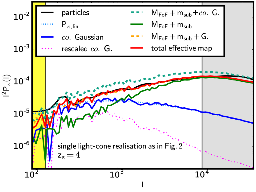
Figure 7: Convergence power spectrum for sources at $z_{s}=4$. The dotted cyan curve shows the predictions using the linear matter power spectrum while the blue line shows the power spectrum of a random Gaussian realisation. The green curve displays the contribution to the power spectrum arising from the haloes $P_{\kappa_{\rm hm}}(l)$ and the dashed orange displays $P_{\kappa_{\rm hm}}(l)+P_{\kappa_{\rm lin}}(l)$, the sum of the halo contribution and the linear Gaussian realisation power-spectra. The black solid line shows the power spectrum of the ray-tracing pipeline using particles from the simulation, while the light-blue dotted line displays the power spectrum of the convergence map calculated summing $\kappa_{\rm hm}$ and $\kappa_{\rm lin}$, a map that is coherent ($co.$) in phase with the halo population. The solid red curve shows the effective total map where the amplitude of $\kappa_{\rm lin}$ is rescaled according to eq. (36) – see the text for more details.

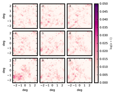
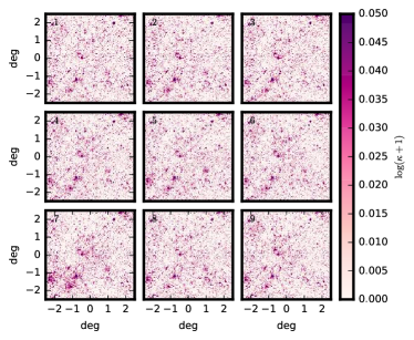
Figure 8: Left panels: nine reconstructed effective linear convergence maps built from the theoretical linear predictions rescaled in amplitude as in eq. (36). Their phase is consistent with the non-linear structures present in the field. Right panels: total effective convergence maps: $\kappa_{\rm hm}+\kappa_{\rm lin}$.

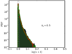
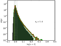
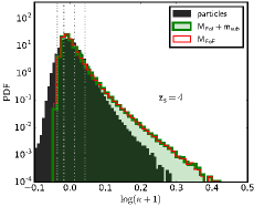
Figure 9: PDF of the convergence maps constructed at three source redshifts. As in Fig. 4 the black histograms present the distribution of the convergence maps built from the ray-tracing pipeline. The green and the red histogram refer to the effective convergence maps build from the FoF groups and the FoF plus subhaloes including also the effective Gaussian linear contribution. Here we show the same light-cone realisation as in Fig. 2 for which we have created $64$ different realisations of the Gaussian linear power spectrum – as an example we have displayed nine of them in Fig. 8.

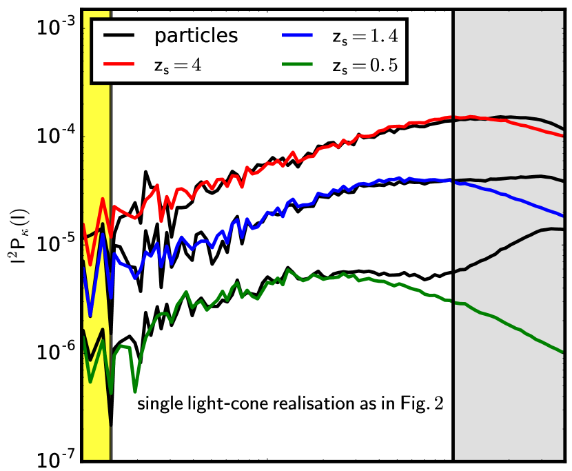
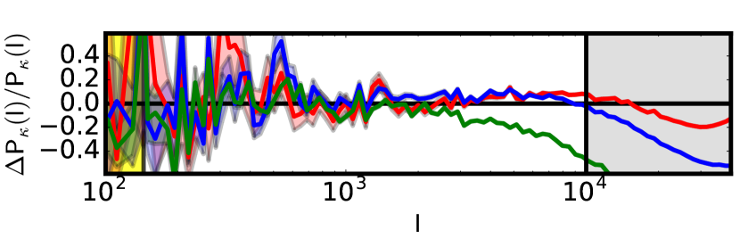
Figure 10: Top panel: convergence power spectra at three different source redshifts of a single light-cone realisation. The black curves show the measurement computed from the ray-tracing using particles while the green, red and blue display the prediction from our halo model algorithm – including FoF haloes and subhaloes – plus the effective linear contribution to resemble the matter density distribution not present in haloes. For the effective linear contribution we have generated $64$ different random Gaussian maps in amplitude all with the same phase and measured the average. Bottom panel: relative difference of the power spectra, the corresponding shaded regions enclose the variance of the power spectra on $64$ different random Gaussian realisation of the effective linear contribution.

4 Statistical Properties of the WL-MOKA_Halo-Model

The effective total maps reconstructed using our halo model reproduce quite well the properties of the maps computed using all the particles in the simulation that are present within the light-cones up to a given source redshift $z_{s}$. The halo and the subhalo catalogues are used to compute the contributions from non-linear structures while the linear power spectrum is used to characterise matter not located in haloes.

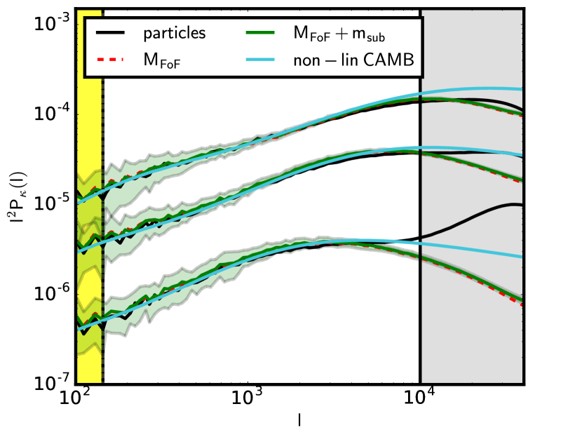
Figure 11: Reconstructed non-linear convergence power spectrum at three different source redshifts: $z_{s}=4$, $z_{s}=1.4$ and $z_{s}=0.5$, from top to bottom, respectively. The black solid lines represent the prediction using the ray-tracing pipeline on the particles within the light-cones. Red dashed lines show the results using Friends-of-Friends haloes, while the green solid lines show the case of FoF haloes plus subhaloes. Shaded green regions enclose the rms of the $25$ light-cones realisations, for each we created $64$ different realisations of the effective linear Gaussian contribution. The cyan curves exhibit the non-linear predictions obtained from CAMB (Lewis et al., 2000), which implements the Takahashi et al. (2012) version of HALOFIT (Smith et al., 2003).

In Fig. 9, we display the PDF of the convergence maps for the first light-cone realisation comparing the effective total maps (haloes – and subhaloes – plus the effective linear term) with the maps computed from particles – as in Fig. 4. For the maps constructed using our WL-MOKA_Halo-Model (where MOKA stands for Matter density distributiOn Kode for gravitationAl lenses) we have generated $64$ random realisations of the amplitude of the effective linear contribution. Left, central and right panels show the results for $z_{s}=0.5$, $1.4$ and $4$, respectively. Again we notice that the PDF of the maps constructed using FoF haloes and subhaloes has a more extended tail toward larger values of the convergence with respect to the maps from simulation: this is due to the fact that they resolve much better the centre of haloes and subhaloes that may suffer from finite mass and force resolution when using particles. Our halo model runs are only limited by the size of the $\kappa$ map we set equal to $2048\times 2048$. This corresponds to approximately $8.8$ arcsec per pixel.. Comparing the green and the red histograms we can notice that including subhaloes the maps present pixels with larger values of the convergence which correspond to the clump cores within FoF groups. From the figure we can also see that the distributions for $\kappa<0$ presents a different sampling of the convergence field: the black histograms are well described by a lognormal tail. In Fig. 10 we show the corresponding convergence power spectra of the same light-cone realisation and source redshifts. Black lines are the measured quantities from the convergence maps computed using particles while green, blue and red curves the corresponding predictions using FoF and subhaloes plus effective Gaussian linear term. As it can be seen in the bottom panel convergence power spectra agree within five percents for angular modes between the Nyquist frequency and $l\approx 10^{4}$. It is interesting to notice that for $z_{s}=0.5$ the particle shot-noise term starts to dominate already at $l\approx 2\times 10^{3}$.

A more detailed comparison between our WL-MOKA_Halo-Model and the ray-tracing analysis can be observed in Fig. 11, where we show the convergence power spectra at three different source redshifts, from top to bottom $z_{s}=4$, $1.4$ and $0.5$, respectively. The black solid curves show the average results of $25$ light-cone realisations from the ray-tracing simulations, the dashed red lines the average cosmic shear power spectrum of our halo model using only the Friends-of-Friends groups while the green curves show the average using FoF with subhaloes. The light-green shaded regions display the rms corresponding to the average measurement of the WL-MOKA_Halo-Model including haloes and subhaloes. The cyan curves are the predictions from CAMB using the prescription of Takahashi et al. (2012) for the non-linear modeling. We would like to underline that possible small departures at small angular modes between our WL-MOKA_Halo-Model predictions and the results from the ray-tracing simulation may be due to the fact that while we generally produce a large sample of Gaussian random realisations of the linear theoretical predictions, in the simulation we have only one random realisation of the initial density field as computed at $z_{i}=99$.

Using cosmic shear measurements to estimate cosmological parameters requires a good knowledge of the covariance matrix, this means information about the correlation and cross-correlation of the lensing measurements between different angular scales, or modes. Typically to have a good sampling of the covariance matrix, we need thousands of independent light-cone realisations of the same field of view and for different initial conditions for the same cosmological model (Taylor & Joachimi, 2014). Using numerical simulations and full ray-tracing analyses, the production of these light-cones requires an enormous amount of computational time and huge storage disk spaces. On the other hand our approximated halo model approach is much faster, not too much demanding in terms of CPU time and little memory consuming, and only requires as input the halo and subhalo catalogues present within the field of view up to the required source redshift plus the linear power spectrum.

From the different light-cones realizations we can write the covariance matrix in Fourier space as:

$$M(l,l^{\prime})=\langle P_{\kappa}(l)-\bar{P}_{\kappa}(l)\rangle\langle P_{\kappa}(l^{\prime})-\bar{P}_{\kappa}(l^{\prime})\rangle$$ (37)

where $\langle\bar{P}_{\kappa}(l)\rangle$ represents the best estimate of the power spectrum at the mode $l$ obtained from the average of all the corresponding light-cone realisations and $P_{\kappa}(l)$ represents the measurement of one realisation. The matrix can be then normalised as follows to obtain the correlation matrix

$$m(l,l^{\prime})=\dfrac{M(l,l^{\prime})}{\sqrt{M(l,l)M(l^{\prime},l^{\prime})}}\,.$$ (38)

For comparison with the $25$ independent light-cones generated from the ray-tracing simulation using particles in the top panels of Fig. 12 we show the correlation matrices of the cosmic shear power spectrum of those different realisations assuming $z_{s}=0.5$, $1.4$ and $4$, from left to right, respectively. We remind the reader that this is presented here only for comparison. On the second row of the figure (in green scale), the three panels show the correlation matrices computed using our WL-MOKA_Halo-Model formalism. We have computed the halo and subhalo contributions from the $25$ different light-cone realisations and for each of them we have generated $64$ effective linear term contribution to represent the matter density distribution that is not in haloes. From the figure, we notice that our halo model reconstructs with very good accuracy the halo sampling properties of the non-linear structures and the contribution from linear theory typically dominant for small values of $l$ within the field of view realization. This sets the basis for the capability of our approach to create self-consistent covariance matrices that can be easily extended to much larger field of view, accounting for a uniform or masked fields of view and considering different geometries and determining how these properties propagate into the lensing measurements and subsequently into the covariance matrices (Harnois-Déraps & van Waerbeke, 2015b).

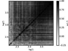
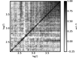
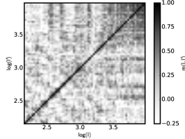
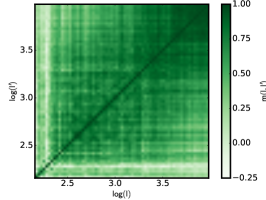
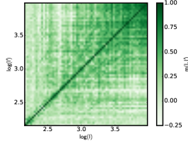
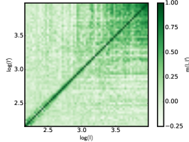
Figure 12: Correlation matrices at three different source redshifts. From left to right $z_{s}=0.5$, $z_{s}=1.4$ and $z_{s}=4$. On the first row, the panels show the correlation matrices of $25$ different light-cone realisations of the ray-tracing pipeline while in the second row are displayed the matrices from the FoF haloes populated with subhaloes plus the effective Gaussian linear contribution. In this case for each light-cone created using the halo model realisation we have generated $64$ random Gaussian effective maps to account for the matter density distribution that is not in haloes.

Before concluding this section we would like to discuss the performance of our halo model-based weak lensing methods in comparison to the full ray-tracing simulation using particles. The first bottle neck in making convergence maps using particles is the construction of the lensing planes and reading the simulation snapshot files. Typically for a $1024^{3}$ dark matter particle simulation the construction of a plane resolving a field of view of $5\times 5$ sq. degrees with $2048^{2}$ pixels takes $2.5$ min that for 22 lens planes up to redshift $z=4$ translates in approximately $60$ min. While the construction of the corresponding halo and subhalo catalogues, reading and projecting the subfind catalogues within the same field of view, takes slightly less then $1.5$ min. The full ray-tracing simulation with glamer on $22$, $14$ and $8$ lens planes, which are needed to construct the convergence maps and measure the convergence power spectrum at $z_{s}=4$, $z_{s}=1.4$ and $z_{s}=0.5$, consumes $70$, $65$ and $62$ min ($8$ threads process), respectively while our halo model code (single thread process) takes $75$ min on haloes in a $5\times 5$ sq. degrees. This time almost doubles when we want to account also for a buffer region of $2.5$ degrees on a side. On a single light cone simulation our fast halo model method is approximately $90\%$ faster than the full ray-tracing simulation using particles. However, it should be stressed that a N-body run from $z=99$ to the present time using the Gadget2 code (Springel, 2005) takes around $50.000$ CPU hours, while a run with an approximate method like Pinocchio (Monaco et al., 2013) takes approximately $750$ hours to generate also the past light-cone up to the desired maximum redshift $z=4$ with our same aperture using a $512^{3}$ grid – on which we can run our fast weak lensing method – while it spends $1550$ CPU hours for the same simulation but using a finer grid of $1024^{3}$ . To summarise, we notice that our fast weak lensing simulation plus an approximate N-body method for the halo catalogue are much faster than the full-ray tracing simulation plus an N-body solver, but still reaching the same level of accuracy in the convergence power spectrum.

5 Summary & Conclusions

In this paper we have presented a self-consistent halo model formalism to construct convergence maps with statistical properties compatible with those derived from the full ray-tracing pipeline.

From the $\Lambda$CDM run of the CoDECS suite we have produced catalogues of haloes and subhaloes present within the constructed matter density light-cones of a field of view of $5\times 5$ sq. degrees up to $z_{s}=4$. To avoid border effects, we stored the information about the haloes and the subhaloes present in a field of view of $10\times 10$ sq. degrees. In the following points we summarise the main ingredients and results of our analyses:

• the mass density distribution in haloes is modelled using the NFW profile. For concentration, we adopt the model by Zhao et al. (2009) for the Friends-of-Friends groups while the Giocoli et al. (2013) function for the $M_{\rm 200}$ mass definition;

• the positive part of the one point statistic of the convergence field is quite well reconstructed using the halo model formalism, however using only the matter present in haloes and subhaloes we are missing the linear matter density field not attached to virialized structures – this means in particular filaments and sheets of the cosmic web;

• the power spectrum of the density field reconstructed with haloes reflects the absence of matter outside haloes, and present less power at large scale than as expected from linear theory;

• the subhalo contribution, using truncated Singular Isothermal Sphere profile, enhances the convergence power spectrum by approximately $3\%$ up to $l\approx 10^{4}$. At smaller scales, this contribution increases dramatically;

• the effective linear contribution on large scales is included by creating a Gaussian field from the theoretical linear cosmic shear power spectrum coherent in phase with the distribution of haloes present in the simulated field of view, renormalizing it in amplitude in order to match the linear prediction on large scales;

• the total effective maps are statistically similar to the ray-tracing ones constructed using the particle density field.

To summarise, our WL-MOKA_Halo-Model formalism self-consistently reconstructs the statistical properties of matter density distribution within light-cones only using the halo and subhalo properties plus the linear power spectrum of the considered cosmological model. When compared with a full ray-tracing simulation using particles for each single realisation, we find an agreement on average within $5\%$ with the reconstructed convergence power spectra for different source redshifts. This highlights the capability of our halo model pipeline in reconstructing the non-linear properties of weak-lensing fields in a much faster way than ray-tracing simulations. Future tests will be dedicated to the capability of extend our method to non-standard cosmologies (Giocoli et al. in preparation) in the light of the recent results presented by (Narikawa et al., 2011; Zhang et al., 2013; Massara et al., 2014; Lombriser et al., 2015; Mead et al., 2016) and also to the possibility to self-consistently develop general models for the cross-correlation between clustering and weak-lensing signals (de la Torre et al., 2016).

Our formalism opens the capacity to create coherent covariance matrices for a given cosmological model and any field of view geometry and masking, allowing a more complete and self-consistent cosmological inspection of realistic lensing data over a wider range of cosmological parameters (de Jong et al., 2013; The Dark Energy Survey Collaboration, 2005; LSST Science Collaboration et al., 2009; Laureijs et al., 2011).

Appendix A Probability Distribution Function of the convergence maps

As discussed in the text, and more in particular displayed in Fig. 9, the comparison of Probability Distribution Function (PDF) between our WL-MOKA_Halo-Model predictions and those using ray-tracing with particles shows some difference that varies as a function of the source redshift. In the discussion we have stressed that this may be due to numerical resolution limits both in force and particle mass that do not allow for resolving well the central part of the haloes and clumps where typically high convergence values appear. However different authors (Taruya et al., 2002; Hilbert et al., 2011; Clerkin et al., 2016; Patton et al., 2016; Xavier et al., 2016) have discussed that the properties of the convergence one point statistic may be characterized by a Gaussian or lognormal distribution. Das & Ostriker (2006) have discussed that small perturbations with resolution of $\theta\sim 10$ arcsec and $z_{s}=1$ account for most of the strong lensing cases and that the PDF is far superior to the Gaussian or the lognormal. They also emphasize that for $z_{s}=4$ about $12\%$ of the strong-lensing cases will result from the contribution of a secondary clump of matter along the line of sight, introducing a systematic error in the determination of the surface density of clusters, typically overestimating it by about some percents.

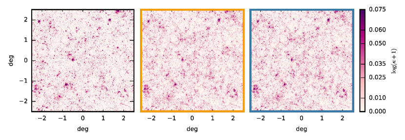
Figure 13: Convergence maps of the light-cone constructed considering sources located at $z_{s}=4$. While the left panel displays the convergence map produced using our WL-MOKA_Halo-Model algorithm, central and right panel show the same realization of the structures with equal phases but forced to have the modulus of the convergence field in the Fourier space $\tilde{\kappa}$ randomly drawn from a Gaussian (central orange framed) and a lognormal (right blue framed) distribution with an identical power spectrum.

In this appendix we discuss the properties of the PDF of the convergence resampling the characteristics of the reconstructed fields in order to have a well defined distribution for the amplitude in the Fourier space $\tilde{\kappa}$ and conserving both the power spectra and the phases to be consistent with non-linear structures. In the left panel of Fig. 13 we display the convergence map reconstructed up to source redshift $z_{s}=4$ using our WL-MOKA_Halo-Model algorithm, the map contains the contributions from haloes, subhaloes and effective linear power spectrum. The central and right panels show two maps that possess the same power spectra and coherent in phase with the left one. However, while in the first (orange framed, termed $resampled_{1}$) the amplitude of the convergence in the Fourier space $\tilde{\kappa}(l)$ is drawn from a Gaussian distribution with rms $\sigma(l)$, in the second (blue framed, termed $resampled_{2}$) the amplitude of $\ln(\tilde{\kappa}+1)$ is drawn from a Gaussian distribution with the rms that can be read as:

$$\sigma^{2}_{\ln}(l)=\ln(\sigma^{2}(l)+1)\,$$ (39)

where $\sigma^{2}(l)=P_{\kappa}(l)$ and $P_{\kappa}(l)$ the convergence power spectrum of the map on the left panel. We then convert the logarithm of the convergence plus one $\widetilde{\ln(\kappa+1)}$ field in the real space and obtain the convergence as

$$\kappa=\exp\left[\ln(\kappa+1)\right]-1\,.$$ (40)

we emphasize that this transformation does generate by construction a lognormal field in real space (Hilbert et al., 2011; Xavier et al., 2016), and we present this case since it produces in real space a map whose PDF is close to the PDF of the case $M_{\rm FoF}+m_{\rm sub}$.

In the three top panels of Fig. 14 we exhibit the PDF of the convergence fields for three different source redshifts, as labelled in the panels. The black histograms show the PDF of the convergence field computed using particles and the glamer pipeline while the green ones the PDF of $64$ realization of the same field using WL-MOKA_Halo-Model: haloes, subhaloes and effective linear power power spectrum contributions. The orange and blue histograms show the Probability Distribution Function of the convergence maps resampled in amplitude in the Fourier space as described above. From the figures we notice that while for low source redshifts the predictions from numerical simulation are quite close to the blue histograms for $z_{s}=4$ the black shaded histogram is very well described by the orange one.

In the three bottom panels we degrade the resolution of the maps to $64\times 64$ pixels which correspond to approximately $281$ arcsec ($l\approx 4.6\times 10^{3}$) in order to remove the particle noise contributions. In all panels the red dashed curves show a lognormal distribution with amplitude equal to half of the first quartile of the black histograms. In those low resolution maps the one point distribution function of the convergence is quite well sampled by the orange histogram, the field is characterized in the Fourier space to have a Gaussian distribution with average zero and variance at a given scale given by the square-root of the predicted convergence power spectrum by our model.

In Figure 15 we display the power spectra of the resampled maps normal and lognormal as discussed above in the text, the orange and the blue curves display the two cases, respectively. From the figure we can notice that since the power spectrum is small compared to unity the differences between the normal and the one that ensures the correct power spectrum for lognormal field is negligible. The curves from top to bottom display the power spectra considering sources at $z_{s}=4$, $z_{s}=1.4$ and $z_{s}=0.5$, respectively.

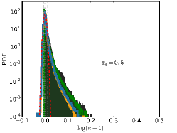
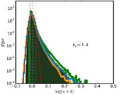
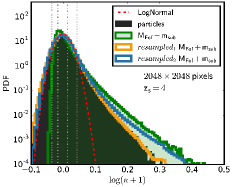
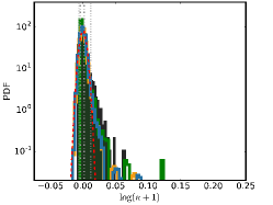
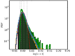
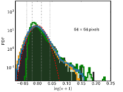
Figure 14: Probability Distribution Function of the convergence field for the three considered source redshifts, $z_{s}=0.5$, $1.4$ and $4$ from left to right, respectively. Top and bottom panels show the PDF of the map resolved with $2048$ and $64$ pixels by side, respectively. In the top panel the pixel size has a resolution of $8.8$ arcsec while in the bottom $281$ arcsec, which correspond to a angular mode of approximately $1.5\times 10^{5}$ and $4.6\times 10^{3}$, respectively.

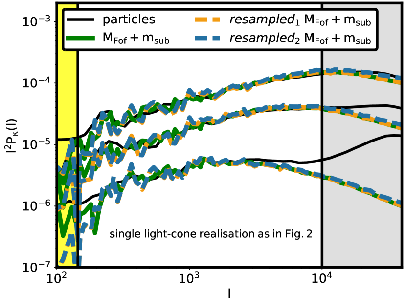
Figure 15: Convergence power spectra for sources at three different redshifts, $z_{s}=0.5$, $1.4$ and $4$ from bottom to top, respectively. Black curves show the power spectrum of the convergence map computed using particles, the green ones using our model which includes FoF-haloes and subhaloes, the dashed orange and blue curves display the power spectra of the resampled maps as discussed in the text.

References

- Angulo & Hilbert (2015) Angulo R. E., Hilbert S., 2015, MNRAS, 448, 364
- Baldi (2012) Baldi M., 2012, MNRAS, 422, 1028
- Bartelmann (1996) Bartelmann M., 1996, A&A, 313, 697
- Bartelmann & Schneider (2001) Bartelmann M., Schneider P., 2001, Physics Reports, 340, 291
- Bartelmann et al. (2012) Bartelmann M., Viola M., Melchior P., Schäfer B. M., 2012, A&A, 547, A98
- Beck et al. (2016) Beck A. M., Murante G., Arth A., Remus R.-S., Teklu A. F., Donnert J. M. F., Planelles S., Beck M. C., Förster P., Imgrund M., Dolag K., Borgani S., 2016, MNRAS, 455, 2110
- Benjamin et al. (2013) Benjamin J., Van Waerbeke L., Heymans C., Kilbinger M., Erben T., Hildebrandt H., Hoekstra H., et al. 2013, MNRAS, 431, 1547
- Bennett et al. (2013) Bennett C. L., Larson D., Weiland J. L., Jarosik N., Hinshaw G., Odegard N., Smith K. M., Hill R. S., et al. G., 2013, ApJS, 208, 20
- Bond et al. (1991) Bond J. R., Cole S., Efstathiou G., Kaiser N., 1991, ApJ, 379, 440
- Bryan & Norman (1998) Bryan G. L., Norman M. L., 1998, ApJ, 495, 80
- Bullock et al. (2001) Bullock J. S., Kolatt T. S., Sigad Y., Somerville R. S., Kravtsov A. V., Klypin A. A., Primack J. R., Dekel A., 2001, MNRAS, 321, 559
- Carbone et al. (2016) Carbone C., Petkova M., Dolag K., 2016, J. Cosmology Astropart. Phys., 7, 034
- Choi et al. (2007) Choi J.-H., Weinberg M. D., Katz N., 2007, MNRAS, 381, 987
- Clerkin et al. (2016) Clerkin L., Kirk D., Manera M., Lahav O., Abdalla F., Amara A., Bacon D., et al. 2016, MNRAS
- Codis et al. (2015) Codis S., Pichon C., Pogosyan D., 2015, MNRAS, 452, 3369
- Cooray & Sheth (2002) Cooray A., Sheth R., 2002, Physics Reports, 372, 1
- Das & Ostriker (2006) Das S., Ostriker J. P., 2006, ApJ, 645, 1
- De Boni et al. (2016) De Boni C., Serra A. L., Diaferio A., Giocoli C., Baldi M., 2016, ApJ, 818, 188
- de Jong et al. (2013) de Jong J. T. A., Kuijken K., Applegate D., Begeman K., Belikov A., Blake C., Bout J., Boxhoorn D., et al. B., 2013, The Messenger, 154, 44
- de la Torre et al. (2016) de la Torre S., Jullo E., Giocoli C., Pezzotta A., Bel J., Granett B. R., Guzzo L., Garilli B., et al. 2016, eprint arXiv: 1612.05647
- Despali et al. (2016) Despali G., Giocoli C., Angulo R. E., Tormen G., Sheth R. K., Baso G., Moscardini L., 2016, MNRAS, 456, 2486
- Diemer et al. (2013) Diemer B., More S., Kravtsov A. V., 2013, ApJ, 766, 25
- Dolag et al. (2004) Dolag K., Bartelmann M., Perrotta F., Baccigalupi C., Moscardini L., Meneghetti M., Tormen G., 2004, A&A, 416, 853
- Duffy et al. (2008) Duffy A. R., Schaye J., Kay S. T., Dalla Vecchia C., 2008, MNRAS, 390, L64
- Eke et al. (1996) Eke V. R., Cole S., Frenk C. S., 1996, MNRAS, 282, 263
- Flaugher (2005) Flaugher B., 2005, International Journal of Modern Physics A, 20, 3121
- Fu et al. (2008) Fu L., Semboloni E., Hoekstra H., Kilbinger M., van Waerbeke L., Tereno I., Mellier Y., Heymans C., Coupon J., Benabed K., Benjamin J., Bertin E., Doré O., Hudson M. J., Ilbert O., Maoli et al. 2008, A&A, 479, 9
- Gao et al. (2008) Gao L., Navarro J. F., Cole S., Frenk C. S., White S. D. M., Springel V., Jenkins A., Neto A. F., 2008, MNRAS, 387, 536
- Gao et al. (2004) Gao L., White S. D. M., Jenkins A., Stoehr F., Springel V., 2004, MNRAS, 355, 819
- Giocoli et al. (2010) Giocoli C., Bartelmann M., Sheth R. K., Cacciato M., 2010, MNRAS, 408, 300
- Giocoli et al. (2016) Giocoli C., Bonamigo M., Limousin M., Meneghetti M., Moscardini L., Angulo R. E., Despali G., Jullo E., 2016, MNRAS, 462, 167
- Giocoli et al. (2016) Giocoli C., Jullo E., Metcalf R. B., de la Torre S., Yepes G., Prada F., Comparat J., Göttlober S., Kyplin A., Kneib J.-P., Petkova M., Shan H. Y., Tessore N., 2016, MNRAS, 461, 209
- Giocoli et al. (2013) Giocoli C., Marulli F., Baldi M., Moscardini L., Metcalf R. B., 2013, MNRAS, 434, 2982
- Giocoli et al. (2012a) Giocoli C., Meneghetti M., Bartelmann M., Moscardini L., Boldrin M., 2012a, MNRAS, 421, 3343
- Giocoli et al. (2015) Giocoli C., Metcalf R. B., Baldi M., Meneghetti M., Moscardini L., Petkova M., 2015, MNRAS, 452, 2757
- Giocoli et al. (2007) Giocoli C., Moreno J., Sheth R. K., Tormen G., 2007, MNRAS, 376, 977
- Giocoli et al. (2012b) Giocoli C., Tormen G., Sheth R. K., 2012b, MNRAS, 422, 185
- Giocoli et al. (2008) Giocoli C., Tormen G., van den Bosch F. C., 2008, MNRAS, 386, 2135
- Guzzo et al. (2014) Guzzo L., Scodeggio M., Garilli B., Granett B. R., Fritz A., Abbas U., Adami C., Arnouts et al. 2014, A&A, 566, A108
- Harnois-Déraps et al. (2012) Harnois-Déraps J., Vafaei S., Van Waerbeke L., 2012, MNRAS, 426, 1262
- Harnois-Déraps & van Waerbeke (2015b) Harnois-Déraps J., van Waerbeke L., 2015b, MNRAS, 450, 2857
- Harnois-Déraps et al. (2015a) Harnois-Déraps J., van Waerbeke L., Viola M., Heymans C., 2015a, MNRAS, 450, 1212
- Hayashi et al. (2003) Hayashi E., Navarro J. F., Taylor J. E., Stadel J., Quinn T., 2003, ApJ, 584, 541
- Heymans et al. (2013) Heymans C., Grocutt E., Heavens A., Kilbinger M., Kitching T. D., Simpson F., Benjamin J., Erben T., et al. 2013, MNRAS, 432, 2433
- Hilbert et al. (2011) Hilbert S., Hartlap J., Schneider P., 2011, A&A, 536, A85
- Hilbert et al. (2009) Hilbert S., Hartlap J., White S. D. M., Schneider P., 2009, A&A, 499, 31
- Hildebrandt et al. (2012) Hildebrandt H., Erben T., Kuijken K., van Waerbeke L., Heymans C., Coupon J., Benjamin J., et al. 2012, MNRAS, 421, 2355
- Hildebrandt et al. (2017) Hildebrandt H., Viola M., Heymans C., Joudaki S., Kuijken K., Blake C., Erben T., Joachimi B., et al. 2017, MNRAS, 465, 1454
- Hirschmann et al. (2014) Hirschmann M., Dolag K., Saro A., Bachmann L., Borgani S., Burkert A., 2014, MNRAS, 442, 2304
- Hockney & Eastwood (1988) Hockney R. W., Eastwood J. W., 1988, Computer simulation using particles
- Ivezic et al. (2008) Ivezic Z., Tyson J. A., Abel B., Acosta E., Allsman R., AlSayyad Y., Anderson S. F., Andrew J., for the LSST Collaboration 2008, eprint arXiv: 0805.2366
- Ivezic et al. (2009) Ivezic Z., Tyson J. A., Axelrod T., Burke D., Claver C. F., Cook K. H., Kahn S. M., Lupton R. H., Monet D. G., Pinto P. A., Strauss M. A., Stubbs C. W., Jones L., Saha A., Scranton R., Smith C., LSST Collaboration 2009, in American Astronomical Society Meeting Abstracts #213 Vol. 41 of Bulletin of the American Astronomical Society, LSST: From Science Drivers To Reference Design And Anticipated Data Products. p. 366
- Jain et al. (2000) Jain B., Seljak U., White S., 2000, ApJ, 530, 547
- Jing (2000) Jing Y. P., 2000, ApJ, 535, 30
- Kainulainen & Marra (2011) Kainulainen K., Marra V., 2011, Phys. Rev. D, 84, 063004
- Kaiser & Squires (1993) Kaiser N., Squires G., 1993, ApJ, 404, 441
- Kaiser et al. (1995) Kaiser N., Squires G., Broadhurst T., 1995, ApJ, 449, 460
- Keeton (2003) Keeton C. R., 2003, ApJ, 584, 664
- Kilbinger et al. (2013) Kilbinger M., Fu L., Heymans C., Simpson F., Benjamin J., Erben T., Harnois-Déraps J., Hoekstra H., Hildebrandt H., et al. 2013, MNRAS, 430, 2200
- Kitching et al. (2014) Kitching T. D., Heavens A. F., Alsing J., Erben T., Heymans C., Hildebrandt H., Hoekstra H., et al. 2014, MNRAS, 442, 1326
- Kitching et al. (2015) Kitching T. D., Heavens A. F., Das S., 2015, MNRAS, 449, 2205
- Köhlinger et al. (2016) Köhlinger F., Viola M., Valkenburg W., Joachimi B., Hoekstra H., Kuijken K., 2016, Mon. Not. Roy. Astron. Soc., 456, 1508
- Lacey & Cole (1993) Lacey C., Cole S., 1993, MNRAS, 262, 627
- Laureijs et al. (2011) Laureijs R., Amiaux J., Arduini S., Auguères J. ., Brinchmann J., Cole R., Cropper M., Dabin C., Duvet L., et al. 2011, eprint arXiv: 1110.3193
- Le Fèvre et al. (2015) Le Fèvre O., Tasca L. A. M., Cassata P., Garilli B., Le Brun V., Maccagni D., Pentericci L., Thomas et al. 2015, A&A, 576, A79
- Lewis et al. (2000) Lewis A., Challinor A., Lasenby A., 2000, Astrophys. J., 538, 473
- Li & Ostriker (2002) Li L.-X., Ostriker J. P., 2002, ApJ, 566, 652
- Lin & Kilbinger (2015a) Lin C.-A., Kilbinger M., 2015a, A&A, 576, A24
- Lin & Kilbinger (2015b) Lin C.-A., Kilbinger M., 2015b, A&A, 583, A70
- Lombriser et al. (2015) Lombriser L., Simpson F., Mead A., 2015, Phys. Rev. Lett., 114, 251101
- LSST Science Collaboration et al. (2009) LSST Science Collaboration Abell P. A., Allison J., Anderson S. F., Andrew J. R., Angel J. R. P., Armus L., Arnett D., Asztalos S. J., Axelrod T. S., et al. 2009, eprint arXiv: 0912.0201
- Massara et al. (2014) Massara E., Villaescusa-Navarro F., Viel M., 2014, J. Cosmology Astropart. Phys., 12, 053
- Mead et al. (2016) Mead A. J., Heymans C., Lombriser L., Peacock J. A., Steele O. I., Winther H. A., 2016, MNRAS, 459, 1468
- Melchior et al. (2011) Melchior P., Viola M., Schäfer B. M., Bartelmann M., 2011, MNRAS, 412, 1552
- Metcalf & Madau (2001) Metcalf R. B., Madau P., 2001, MNRAS, 563, 9
- Metcalf & Petkova (2014) Metcalf R. B., Petkova M., 2014, MNRAS, 445, 1942
- Mohammed et al. (2014) Mohammed I., Martizzi D., Teyssier R., Amara A., 2014, eprint arXiv: 1410.6826
- Monaco (2016) Monaco P., 2016, Galaxies, 4, 53
- Monaco et al. (2013) Monaco P., Sefusatti E., Borgani S., Crocce M., Fosalba P., Sheth R. K., Theuns T., 2013, MNRAS, 433, 2389
- Moore et al. (1998) Moore B., Governato F., Quinn T., Stadel J., Lake G., 1998, ApJ, 499, L5+
- Narikawa et al. (2011) Narikawa T., Kimura R., Yano T., Yamamoto K., 2011, International Journal of Modern Physics D, 20, 2383
- Navarro et al. (1996) Navarro J. F., Frenk C. S., White S. D. M., 1996, ApJ, 462, 563
- Neto et al. (2007) Neto A. F., Gao L., Bett P., Cole S., Navarro J. F., Frenk C. S., White S. D. M., Springel V., Jenkins A., 2007, MNRAS, 381, 1450
- Pace et al. (2015) Pace F., Baldi M., Moscardini L., Bacon D., Crittenden R., 2015, MNRAS, 447, 858
- Patton et al. (2016) Patton K., Blazek J., Honscheid K., Huff E., Melchior P., Ross A. J., Suchyta E., 2016, eprint arXiv: 1611.01486
- Percival et al. (2014) Percival W. J., Ross A. J., Sánchez A. G., Samushia L., Burden A., Crittenden R., Cuesta A. J., et al. 2014, MNRAS, 439, 2531
- Petkova et al. (2014) Petkova M., Metcalf R. B., Giocoli C., 2014, MNRAS, 445, 1954
- Petri et al. (2016a) Petri A., Haiman Z., May M., 2016a, eprint arXiv: 1612.00852
- Petri et al. (2016b) Petri A., Haiman Z., May M., 2016b, Phys. Rev. D, 93, 063524
- Planck Collaboration (2016) Planck Collaboration 2016, Astron. Astrophys., 594, A13
- Prada et al. (2016) Prada F., Scóccola C. G., Chuang C.-H., Yepes G., Klypin A. A., Kitaura F.-S., Gottlöber S., Zhao C., 2016, MNRAS, 458, 613
- Rasia et al. (2004) Rasia E., Tormen G., Moscardini L., 2004, MNRAS, 351, 237
- Roncarelli et al. (2007) Roncarelli M., Moscardini L., Borgani S., Dolag K., 2007, MNRAS, 378, 1259
- Sato et al. (2009) Sato M., Hamana T., Takahashi R., Takada M., Yoshida N., Matsubara T., Sugiyama N., 2009, ApJ, 701, 945
- Schäfer et al. (2012) Schäfer B. M., Heisenberg L., Kalovidouris A. F., Bacon D. J., 2012, MNRAS, 420, 455
- Sheth & Jain (2003) Sheth R. K., Jain B., 2003, MNRAS, 345, 529
- Sheth & Tormen (1999) Sheth R. K., Tormen G., 1999, MNRAS, 308, 119
- Sheth & Tormen (2004a) Sheth R. K., Tormen G., 2004a, MNRAS, 349, 1464
- Sheth & Tormen (2004b) Sheth R. K., Tormen G., 2004b, MNRAS, 350, 1385
- Smith et al. (2003) Smith R. E., Peacock J. A., Jenkins A., White S. D. M., Frenk C. S., Pearce F. R., Thomas P. A., Efstathiou G., Couchman H. M. P., 2003, MNRAS, 341, 1311
- Sousbie et al. (2008) Sousbie T., Pichon C., Colombi S., Novikov D., Pogosyan D., 2008, MNRAS, 383, 1655
- Sousbie et al. (2011) Sousbie T., Pichon C., Kawahara H., 2011, MNRAS, 414, 384
- Spergel et al. (2013) Spergel D., Gehrels N., Breckinridge J., Donahue M., Dressler A., Gaudi B. S., Greene T., Guyon O., Hirata C., et al. K., 2013, eprint arXiv: 1305.5422
- Springel (2005) Springel V., 2005, MNRAS, 364, 1105
- Springel et al. (2001b) Springel V., White S. D. M., Tormen G., Kauffmann G., 2001b, MNRAS, 328, 726
- Takahashi et al. (2012) Takahashi R., Sato M., Nishimichi T., Taruya A., Oguri M., 2012, ApJ, 761, 152
- Taruya et al. (2002) Taruya A., Takada M., Hamana T., Kayo I., Futamase T., 2002, ApJ, 571, 638
- Tassev et al. (2013) Tassev S., Zaldarriaga M., Eisenstein D. J., 2013, J. Cosmology Astropart. Phys., 6, 36
- Taylor & Joachimi (2014) Taylor A., Joachimi B., 2014, MNRAS, 442, 2728
- Tessore et al. (2015) Tessore N., Winther H. A., Metcalf R. B., Ferreira P. G., Giocoli C., 2015, J. Cosmology Astropart. Phys., 10, 036
- The Dark Energy Survey Collaboration (2005) The Dark Energy Survey Collaboration 2005, eprint ArXiv: astro-ph/0510346
- Tinker et al. (2008) Tinker J., Kravtsov A. V., Klypin A., Abazajian K., Warren M., Yepes G., Gottlöber S., Holz D. E., 2008, ApJ, 688, 709
- Vale & White (2003) Vale C., White M., 2003, ApJ, 592, 699
- van Daalen & Schaye (2015) van Daalen M. P., Schaye J., 2015, MNRAS, 452, 2247
- van den Bosch (2002) van den Bosch F. C., 2002, MNRAS, 331, 98
- Viola et al. (2011) Viola M., Melchior P., Bartelmann M., 2011, MNRAS, 410, 2156
- Wechsler et al. (2002) Wechsler R. H., Bullock J. S., Primack J. R., Kravtsov A. V., Dekel A., 2002, ApJ, 568, 52
- Xavier et al. (2016) Xavier H. S., Abdalla F. B., Joachimi B., 2016, MNRAS, 459, 3693
- Yu et al. (2016) Yu Y., Zhang P., Jing Y., 2016, Phys. Rev., D94, 083520
- Zel’Dovich (1970) Zel’Dovich Y. B., 1970, A&A, 5, 84
- Zhang et al. (2013) Zhang Y., Zhang P., Yang X., Cui W., 2013, Phys. Rev. D, 87, 023521
- Zhao et al. (2009) Zhao D. H., Jing Y. P., Mo H. J., Bnörner G., 2009, ApJ, 707, 354
- Zhao et al. (2003b) Zhao D. H., Jing Y. P., Mo H. J., Börner G., 2003b, ApJ, 597, L9
- Zhao et al. (2003a) Zhao D. H., Mo H. J., Jing Y. P., Börner G., 2003a, MNRAS, 339, 12
- Zorrilla Matilla et al. (2016) Zorrilla Matilla J. M., Haiman Z., Hsu D., Gupta A., Petri A., 2016, Phys. Rev. D, 94, 083506