Spin-polarized tunneling into helical edge states: asymmetry and conductances

Abstract

We consider tunneling from the spin-polarized tip into the Luttinger liquid edge state of quantum spin Hall system. This problem arose in context of the spin and charge fractionalization of an injected electron. Renormalization of the dc conductances of the system is calculated in the fermionic approach and scattering states formalism. In lowest order of tunneling amplitude we confirm previous results for the scaling dependence of conductances. Going beyond the lowest order we show that interaction affects not only the total tunneling rate, but also the asymmetry of the injected current. The helical edge state forbids the backscattering, which leads to the possibility of two stable fixed points in renormalization group sense, in contrast to the Y-junction between the usual quantum wires.

I Introduction

Topological insulators (TI) is a class of materials apparently important for future electronic devices. Hasan and Kane (2010); Qi and Zhang (2011) Being an insulator in the bulk, the TI necessarily has conducting states on its edge. The spin-orbit interaction leads to electrons spin-momentum locking in the edge states creating so called helical states. Backscattering on the nonmagnetic impurities in the same channel of such edge states is absent due to TI time-reversal symmetry. It allows a creation of devices with a lossless electron transport.

Electrons on the edge of 2D TI are confined to one spatial dimension (1D). One dimensional electron transport near the Fermi energy is described by well-known Tomonoga-Luttinger liquid (TLL) model. Giamarchi (2004) The TLL corresponds to strongly correlated electron matter, and the 1D helical edge states add new peculiarities to it. This explains large experimental and theoretical interest to helical TLLs, with several suggested ways of probing their strongly correlated nature. Investigating the helical edge states was theoretically proposed by means of magnetic field in Braunecker et al. (2012); Kharitonov (2012); Soori et al. (2012), by specific spatial construction of helical state in Dolcetto et al. (2013a); Calzona et al. (2015a); Calzona et al. (2016) and by quantum dots in Chao et al. (2013); Dolcetto et al. (2013b).

Another natural way of probing – tunneling from the tip into the edge state – attracted a lot of attention. There is experimental evidence Steinberg et al. (2007) and theoretical explanation Hur et al. (2008) that the electron injection even into usual TLL may be characterized by charge fractionalization resulting in the currents imbalance. For helical TLL probing by the tip was considered theoretically in papers Pugnetti et al. (2009); Das and Rao (2011); Garate and Le Hur (2012); Khanna et al. (2013); Calzona et al. (2015b); Santos et al. (2016). Experimentally it was confirmed that TI edge state is a quantum spin Hall state Kim et al. (2014) , helical behavior of the edge state was observed in Li et al. (2015), the STM experiments were reported in Pauly et al. (2015); Wu et al. (2016).

The transport properties of TLL model may be studied in two main approaches. The bosonization approach Giamarchi (2004) takes into account the electron interaction exactly, the impurities are regarded as perturbation. The fermionic approach treats interaction perturbatively and studies the renormalization of impurities/junctions in $S$-matrix formalism of asymptotic electronic states. Transport in quantum point contact is described by the conductances (transparencies) of junctions. The problem with one impurity in quantum wire can also be interpreted as the point contact of two wires. The latter case was considered within the TLL model in bosonization Giamarchi and Schulz (1988); Furusaki and Nagaosa (1993); Kane and Fisher (1992) and fermionic Matveev et al. (1993); Yue et al. (1994) approaches. The conclusion of both approaches is that repulsive interaction renormalizes bare conductance to zero (total reflection case) whereas the attractive interaction leads to perfect transmission in the low temperature limit.

Further studies of usual TLL in bosonization approach addressed Y-junction with equal interaction constant Oshikawa et al. (2006) and arbitrary interaction in three wires Hou et al. (2012). The corner junction of helical TLLs was considered for two TI’s in  Hou et al. (2009); Teo and Kane (2009); Ström and Johannesson (2009).

In the fermionic approach the renormalization group (RG) equations for $S$-matrix characterizing the junction for arbitrary number of quantum wires was presented in  Lal et al. (2002); Das et al. (2004). Conductances of Y and X junctions were analyzed in the first order of interaction.

A partial summation of the perturbation series was performed in Aristov and Wölfle (2009) in order to recover the exact scaling exponents for conductance for one impurity. The results were used for the RG analysis of Y-junction  Aristov (2011); Aristov and Wölfle (2012a); Aristov and Wölfle (2013) and generalized to arbitrary number of wires  Aristov and Wölfle (2012b). The contact of two helical TLL and tunneling from unpolarized spinful wire into the helical edge state were considered in  Aristov and Niyazov (2016). The agreement between bosonization and fermionic approaches has been obtained when the comparison was available.

In the present letter we focus on the spin-polarized tunneling into the helical edge state. This problem was previously studied within bosonization approach Das and Rao (2011), with the setup consisting of a point contact between fully spin-polarized tip and the helical edge state (see Fig.1). Generally, spin polarization in the tip differs from the spin direction of the edge state fermions by some angle, $\xi$. In the absence of interaction this angle defines the left-right current asymmetry of the injected current. The charge fractionalization was demonstrated for the injection of electrons even with polarization parallel to the edge states in case of infinite helical TLL without Fermi liquid leads. Generalization of this result to time-dependent injected pulses was done in Garate and Le Hur (2012). The effect of metallic leads for the visibility of fractionalization phenomena in transport measurement in helical TLL was analyzed in  Calzona et al. (2015b). It was argued there that the fractionalization cannot be observed for dc currents, while information about helical TLL physics can be extracted from studying the transient dynamics.

In our approach below we use the fermionic formalism of scattering states, which implies the existence of Fermi liquid leads. It results in the absence of charge fractionalization in dc limit for the parallel polarization of the tip. For non-parallel polarization we show that the left-right asymmetry of the dc current, injected into helical TLL, is not defined entirely by the polarization angle but is renormalized along with the total tunneling conductance, with the resulting coupled RG equations. The asymmetry renormalization appears in first order of interaction strength and first order of tunneling conductance, and we discuss it in detail. Simultaneous renormalization of two quantities is tied to the existence of saddle point RG fixed point (FP) in the phase portrait of the system. Aristov et al. (2010) In the absence of backscattering in the helical TLL, this non-universal FP separates two truly stable FPs. This in turn may lead to qualitatively different renormalization of asymmetry and the total tunneling rate for different interaction strength.

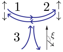
Figure 1: Schematically shown scanning tunneling microscopy of the helical edge state of topological insulator by the spin-polarized tip. $\xi$ is an angle between electron spin in the tip and spin quantization axis of the helical state.

II Theoretical formalism

II.1 The model

We consider Y-junction of the quantum wires shown in Fig. 1. Two quantum wires labeled by $j=1,2$ correspond to the TI helical edge state and the wire with $j=3$ is the tunneling tip with fully polarized electrons. The polarization vector of electrons in the tip is different from the quantization axis in the TI edge state. We denote this difference by the angle $\xi$, so that $\xi=0(\pi)$ describes the tip polarization parallel (antiparallel) to the right-moving fermions in the edge state.

The helical state of the main wire is described by the TLL model with the interaction between electrons of short-range forward-scattering type. All three quantum wires of length $L$ are adiabatically connected to the reservoirs or leads such that additional scattering is absent. Scattering electron states flowing in and out the junction are connected by the $S$ matrix.

TLL model Hamiltonian with linearized spectrum near the Fermi energy and in the scattering states formalism reads

$$\mathcal{H} =\int_{0}^{\infty}dx[H^{0}+H^{int}\Theta(\ell<x<L)]\,,$$ (1)

$$H^{0} =v_{F}\Psi_{in}^{\dagger}i\nabla\Psi_{in}-v_{F}\Psi_{out}^{\dagger}i\nabla\Psi_{out}\,,$$

$$H^{int} =2\pi v_{F}\sum\limits_{j=1}^{3}g_{j}\widehat{\rho}_{j}\widehat{\widetilde{\rho}}_{j}\,.$$

Density operators are defined by $\widehat{\rho}_{j,in}=\Psi^{+}\rho_{j}\Psi=\widehat{\rho}_{j}$, and $\widehat{\rho}_{j,out}=\Psi^{+}\widetilde{\rho}_{j}\Psi=\widehat{\widetilde{\rho}}_{j}$, where $\widetilde{\rho}_{j}=S^{+}\cdot\rho_{j}\cdot S$ and the density matrices are given by $(\rho_{j})_{\alpha\beta}=\delta_{\alpha\beta}\delta_{\alpha j}$ and $(\widetilde{\rho}_{j})_{\alpha\beta}=S_{\alpha j}^{+}S_{j\beta}$. Electron interaction constant in the edge state is defined by $g_{1}=g_{2}=g$ and $g_{3}=0$ in the tip ; we set $v_{F}=1$ below. Here we introduce window function $\Theta(\ell<x<L)$ such that $\Theta(x)=1$, if $\ell<x<L$ and zero otherwise. The ultraviolet cutoff at $x=\ell$ is required for our model point-like interaction, $H^{int}$, and for finite-range interaction $\ell$ is associated with the screening length, see Appendix B.

Ingoing and outgoing electronic waves $\psi_{j,\text{in}},\psi_{j,\text{out}}$ are connected at the junction by the $S$ matrix $\Psi_{out}(x)=S\cdot\Psi_{in}(x)$ at $x\to 0$, where $\Psi_{in(out)}=(\psi_{1,in(out)},\psi_{2,in(out)},\psi_{3,in(out)})$. The $S$-matrix characterizes the scattering in the junction and belongs to the unitary group $U(3)$. Our setup implies the chiral property, $|S_{13}|=|S_{32}|$, $|S_{23}|=|S_{31}|$. Due to the time-reversal invariance of TI, the backscattering in the edge state without the tip is forbidden. The same is true in case in which the polarization of the tip is parallel to the spin direction of right or left mover, $\xi=0,\pi$.

In general, the chiral S-matrix is characterized by three parameters Aristov and Wölfle (2013). The absence of backscattering reduces the appropriate $S$ matrix to the following two-parametric form

$$S =\begin{pmatrix}r_{1}&t_{12}&t_{13}\\ t_{21}&r_{1}&t_{23}\\ t_{31}&t_{32}&r_{2}\\ \end{pmatrix}$$ (2)

$$r_{1} =\sin^{2}\frac{\theta}{2}\sin\xi,\quad r_{2}=\cos\theta,$$

$$t_{12} =-\cos\theta\cos^{2}\frac{\xi}{2}-\sin^{2}\frac{\xi}{2},\quad t_{21}=t_{12}|_{\xi\rightarrow\pi-\xi},$$

$$t_{13} =t_{32}=\cos\frac{\xi}{2}\sin\theta,\quad t_{23}=t_{31}=\sin\frac{\xi}{2}\sin\theta.$$

One parameter, $\theta$, is responsible for the tunneling amplitude and $\theta=0$ corresponds to the fully detached tip, in this case there is a perfect transmission through the edge state. Second parameter $\xi$ is the above angle between electron spin in the tip and spin quantization axis of the helical state (see Appendix A).

II.2 Reduced conductances

In the linear response regime the conductances are defined by $I_{i}=C_{ik}V_{k}$ where $I_{j}$ and $V_{j}$ are the current flowing towards in the junction and the electric potential in $j$th lead, respectively. In the dc limit one easily obtains from Kubo formula $C_{ij}=\delta_{ij}-Y_{ij}$, with $Y_{ij}=|S_{ij}|^{2}$. The total current conservation and the absence of current for equal voltages lead to conditions $\sum_{i}C_{ij}=\sum_{j}C_{ij}=0$, which also stem from the unitarity of $S$-matrix. This means that we can introduce new current and voltage combinations to show the condition explicitly. Aristov and Wölfle (2011)

We choose new combinations according to relations $I_{i}^{\text{new}}=\sum_{k}R_{ki}I_{k}$, $V_{i}^{\text{new}}=\sum_{k}R_{ki}V_{k}$, where the matrix

$$\mathbf{R}=\begin{pmatrix}\frac{1}{\sqrt{2}}&\frac{1}{\sqrt{6}}&\frac{1}{\sqrt{3}}\\ -\frac{1}{\sqrt{2}}&\frac{1}{\sqrt{6}}&\frac{1}{\sqrt{3}}\\ 0&-\sqrt{\frac{2}{3}}&\frac{1}{\sqrt{3}}\end{pmatrix}$$ (3)

has properties $\mathbf{R}^{-1}=\mathbf{R}^{T}$, $\mbox{det }\mathbf{R}=1$.

The corresponding matrix of conductances $\mathbf{C}^{R}=\mathbf{R}^{T}\,\mathbf{C}\,\mathbf{R}$ for the above form of $S$, Eq. (2), becomes

$$\mathbf{C}^{R}=\begin{pmatrix}1-a&-c&0\\ c&1-b&0\\ 0&0&0\end{pmatrix}.$$ (4)

with

$$a =\tfrac{1}{2}(1+\cos^{2}\theta)\cos^{2}\xi-\cos\theta\sin^{2}\xi,$$ (5)

$$b =\tfrac{1}{4}(1+3\cos 2\theta),$$

$$c =\tfrac{\sqrt{3}}{2}\cos\xi\sin^{2}\theta.$$

It is convenient to analyze the quantity $\mathbf{Y}^{R}=1-\mathbf{C}^{R}$ below. Clearly, only two components of $\mathbf{Y}^{R}$ are independent. The chiral component of conductance, $c$, depends on the asymmetry parameter, $\cos\xi$, which includes the polarization angle, $\xi$.

We can also introduce more “physical” combinations of currents, $\mathbf{I}^{\text{phys}}=(I_{a},I_{b})$, and voltages, $\mathbf{V}^{\text{phys}}=(V_{a},V_{b})$, as

$$I_{a} =\tfrac{1}{2}(I_{1}-I_{2})\,,\quad I_{b}=\tfrac{1}{3}(I_{1}+I_{2}-2I_{3})\,,$$ (6)

$$V_{a} =V_{1}-V_{2}\,,\quad V_{b}=\tfrac{1}{2}(V_{1}+V_{2}-2V_{3})\,.$$

In terms of these, the matrix of conductances $\mathbf{I}^{\text{phys}}=\mathbf{G}\mathbf{V}^{\text{phys}}$ is given by

$$\mathbf{G}=\begin{pmatrix}G_{a}&G_{ab}\\ G_{ba}&G_{b}\end{pmatrix}=\begin{pmatrix}\frac{1}{2}(1-a)&-\frac{c}{\sqrt{3}}\\ \frac{c}{\sqrt{3}}&\frac{2}{3}(1-b)\end{pmatrix}.$$ (7)

with the property, $0\leq G_{a,b}\leq 1$, see Aristov and Wölfle (2011).

II.3 Renormalization group equations

The dc transport through the chiral Y-junction was studied in fermionic formalism in Aristov and Wölfle (2012a); Aristov and Wölfle (2013). We sketch here the derivation of the corresponding formulas. The principal first order interaction correction to the conductances reads Aristov and Wölfle (2012a)

$$C_{jk}=C_{jk}\big{\rvert}_{\mathbf{g}=0}+\tfrac{1}{2}\sum\limits_{l,m}\mbox{Tr}\left[\widehat{W}_{jk}\widehat{W}_{lm}\right]g_{ml}\Lambda\,,$$ (8)

where we defined $C_{jk}\rvert_{\mathbf{g}=0}=\delta_{jk}-Y_{jk}$, a matrix $g_{ml}=g_{l}\delta_{ml}$ with interaction constants $g_{l}$ in the Hamiltonian (1), nine $3\times 3$ matrices $\widehat{W}_{jk}=[\rho_{j},\widetilde{\rho}_{k}]$ and the trace operation Tr is defined with respect to the 3$\times$3 matrix space of $\widehat{W}$’s. The scale-dependent term $\Lambda=\ln(\min[L,\xi]/\ell)$ with the temperature correlation length $\xi=v_{F}/T$.

The above correction is the leading contribution, $\sim g\Lambda$, to conductance. It was shown Aristov and Wölfle (2011) that the higher-order corrections obey the scaling hypothesis for the conductance and are generated by a set of the differential RG equations. In its simplest form, these equations are obtained by differentiating Eq. (8) over $\Lambda$ (and then putting $\Lambda=0$) which gives

$$\frac{d}{d\Lambda}Y_{jk}^{R}=-\frac{1}{2}\sum\limits_{l,m}\mbox{Tr}\left[\widehat{W}_{jk}^{R}\widehat{W}_{lm}^{R}\right]g_{ml}^{R}\,,$$ (9)

where all quantities with superscript $R$ are defined as $\mathbf{A}^{R}=\mathbf{R}^{T}\,\mathbf{A}\,\mathbf{R}$.

The main source of linear-in-$\Lambda$ subleading corrections corresponds to a ladder series of diagrams, which can be summed analytically Aristov and Wölfle (2011). These corrections are independent of the scheme of regularization in RG procedure and lead to the scaling exponents for conductances, coinciding with those obtained by bosonization method.

The result of the ladder summation Aristov and Wölfle (2012b); Aristov and Wölfle (2013) is the RG equation similar to above Eq.  (9) with the replacement

$$\mathbf{g}\to\bar{\mathbf{g}}=2(\mathbf{Q}-\mathbf{Y})^{-1}\,.$$ (10)

The matrix $\mathbf{Q}$ depends on the Luttinger parameters $K_{j}$ of individual wires and has the form

$$Q_{jk} =q_{j}\delta_{jk}\,,\quad q_{j}=(1+K_{j})/(1-K_{j})\,,$$ (11)

$$K_{j} =[(1-g_{j})/(1+g_{j})]^{1/2}.$$

In our case we have $g_{1}=g_{2}=g$ and $g_{3}=0$. The latter equality corresponds to $q_{3}\to\infty$, whose limit is easily taken in (10).

Now we are in a position to obtain RG equations of the conductances. However, the equivalent RG equations in terms of parametrization (2) have simpler form, and we choose it below. After some algebra we obtain from (5), (9), (10) the following set of equations

$$\frac{d\theta}{d\Lambda} =-\frac{1}{8}(1-K)\sin\theta\frac{F_{1}(\theta)+F_{2}(\theta)\cos 2\xi}{F_{3}(\theta)D(\theta,\xi)},$$ (12)

$$\frac{d\xi}{d\Lambda} =\frac{1}{4}(1-K)\frac{(1-\cos\theta)\sin 2\xi}{D(\theta,\xi)},$$

$$F_{1} =2(1-K)-(3-K)\sin^{2}\frac{\theta}{2}$$

$$-3(1-K)\sin^{2}\theta,$$

$$F_{2} =\sin^{2}\frac{\theta}{2}(2-3(1-K)\sin^{2}\frac{\theta}{2}),$$

$$F_{3} =1-(1-K)\sin^{2}\frac{\theta}{2},$$

$$D(\theta,\xi) =K+(1-K)\sin^{2}\frac{\theta}{2}\left(1-\sin^{2}\frac{\theta}{2}\sin^{2}\xi\right).$$

These equations are analyzed in the next section. Notice that the asymmetry parameter $p=\cos\xi$ is now determined not only by the initial polarization angle, but also by the interaction strength and tunneling amplitude.

III Spin-polarized tunneling

III.1 Lowest order calculation

Let us first consider the limit of weak tunneling into the helical edge state. This means that both tunneling from the tip and the backscattering in the edge state due to this tunneling are approximately zero. In terms of the $S$-matrix (2) we write $|r_{2}|^{2}\simeq 1$ and $|r_{1}|^{2}\simeq 0$. First condition gives $\theta\simeq 0$ or $\theta\simeq\pi$, and the second condition states that if $\theta\simeq\pi$ then $\xi\simeq 0$ or $\xi\simeq\pi$. These three seemingly unconnected regions form a neighborhood of the fixed point (FP) A, as is discussed below.

Confining ourselves to the linear-in- $\theta$ terms, we get from Eqs. (12):

$$\frac{d\theta}{d\Lambda} =-\frac{(1-K)^{2}}{4K}\theta\,,\qquad\frac{d\xi}{d\Lambda}=0\,.$$ (13)

Hence, the parameter $\theta$, which is related to the barrier transparency, is renormalized to zero with the scaling law $\theta=\theta_{0}\exp(-\nu\Lambda/2)$, and the tunneling exponent $\nu=(1-K)^{2}/2K$. The asymmetry ratio $t_{\downarrow}/t_{\uparrow}=\tan\xi/2$ is not renormalized.

This result is in exact agreement with the earlier work Das and Rao (2011), where the renormalization of the tunnel amplitudes $t_{\uparrow}$ and $t_{\downarrow}$ was studied in the bosonization approach. Equation (9) of the above paper obtains the currents flowing to the right $I_{\text{R}}$ and to the left $I_{\text{L}}$ ends of the edge state. One has

$$I_{\text{L}}+I_{\text{R}} =I_{0}\,,\qquad I_{\text{L}}-I_{\text{R}}=-KI_{0}\cos\xi\,.$$ (14)

In our notation  (6) the current $I_{0}$ equals to $I_{b}$, and the difference of the currents $I_{\text{L}}-I_{\text{R}}$ is $2I_{a}$. For zero bias in the edge state, $V_{a}=0$, we have $I_{b}=G_{b}V_{b}$, $I_{a}=G_{ab}V_{b}$ and obtain from Eqs.  (5), (7) :

$$2I_{a}=-I_{b}\cos\xi$$ (15)

This equation coincides with (14) apart from the factor $K$, which is absent in dc limit in our setup with the Fermi leads. The absence of this factor in the similar setup was also obtained in the work  Calzona et al. (2015b) in bosonization approach.

Now we consider the next terms in the expansion of RG equations in $\theta$. Quadratic-in $\theta$ term appears only in RG equation for asymmetry angle:

$$\frac{d\xi}{d\Lambda}=\frac{1-K}{8K}\theta^{2}\sin 2\xi.$$ (16)

Solution of the equation shows that the asymmetry angle is renormalized according to the law

$$\tan\xi=\tan\xi_{0}e^{-(\theta^{2}-\theta_{0}^{2})/2(1-K)}.$$ (17)

Since $\theta$ is renormalized to zero (see eq. (13)), we find the whole renormalization of $\xi$ insignificant for small bare tunneling amplitude $\theta_{0}$. At the same time the renormalization of $\xi$ in (16) is first order interaction effect for small interaction $\frac{1-K}{K}\approx g\ll 1$, whereas the tunneling exponent for $\theta$ in Eq. (13) is given by the second order of interaction, $\frac{(1-K)^{2}}{K}\approx g^{2}$.

We see that if we discard the small-in-$\theta$ terms in RG equation for $\xi$, then we do not obtain renormalization of asymmetry at all. However the smallness-in-$\theta$ may be compensated by the less power of interaction in the RG flow of $\xi$. As a result for small interaction and tunneling amplitude the renormalization of $\theta$ and $\xi$ may be of the same order as demonstrated in Fig. 2.

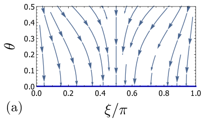
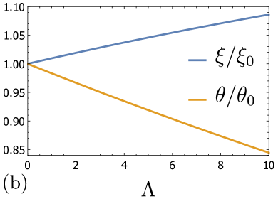
Figure 2: The panel (a) shows RG flows in the plane $(\xi,\ \theta)$ for $g=0.26$ ($K=0.77$). Relative renormalization of $\xi$ and $\theta$ for the flow with $\xi_{0}=0.3$, $\theta_{0}=0.4$ is shown in panel (b).

We also note here that Eq.  (17) can be rewritten in terms of the asymmetry $p=\cos\xi=-2I_{a}/I_{b}$ as

$$\frac{dp}{d\Lambda}=-\frac{1-K}{4K}\theta^{2}p(1-p^{2}).$$ (18)

This equation possesses three fixed points (FPs) $p=0,\pm 1$, and if $\theta^{2}$ were non-vanishing at $\Lambda\to\infty$, then we would obtain only $p=0$ as a stable FP for repulsive interaction, $K<1$. In the leading order of interaction, we can combine first equation in (13) and (18) to represent the RG trajectory in the form

$$\theta^{2}-g\log\frac{p^{2}}{1-p^{2}}=\mbox{const}.$$ (19)

III.2 M point

The terms of the order $\theta^{3}$ appear only in the equation for $\theta$ :

$$\frac{d\theta}{d\Lambda}=-\frac{(1-K)^{2}}{4K}\theta+\frac{(1-K)(\kappa-\cos 2\xi)}{16K}\theta^{3},$$ (20)

where $\kappa\equiv(1-K)(2/3+K)+1/K$. For small interaction $\kappa\approx 1$ and the equation (20) becomes

$$\frac{d\theta}{d\Lambda}=-\frac{g^{2}}{4}\theta+\frac{g(1-\cos 2\xi)}{16}\theta^{3}.$$ (21)

First, one can see here that the $\theta^{3}$ -term is unimportant in parallel polarization case, $\xi=0,\pi$; the right-hand side of Eq. (16) is zero. Thus the lines $\xi=0,\pi$ are RG fixed lines.

Otherwise the combination of (20) with (16) reveals the existence of non-universal fixed point M at $\xi_{M}=\pi/2$, $\theta_{M}\approx\sqrt{2g}$. Similar to above Eq. (16), the next-order term in $\theta$ expansion contains smaller power of interaction strength. This situation was discussed for non-chiral symmetric Y-junction in Aristov et al. (2010).

Solving RG equations for asymmetry $p$ and $\theta$ gives for the RG trajectory

$$\theta^{2}p-g\log\frac{1+p}{1-p}=\mbox{const}\,.$$ (22)

Despite the apparently different form of Eqs.  (22) and (19), these equations yield numerically close curves for small $\theta<\theta_{M}$. Indeed the existence of the next term in equation (20) does not seriously affect RG flows in this limit.

Already at the level of approximate Eqs.  (20), (16) one can expect that for $\theta\approx\theta_{M}$ the RG flow for the asymmetry $\cos\xi$ may exceed the RG flow of barrier transparency $\theta$. We discuss this point in more detail in the next subsection.

III.3 Non-perturbative RG results

Now we go beyond the weak tunneling approximation and discuss the general RG Eqs. (12) for $K<1$. In this rather complicated case we have five universal FPs in the $(\theta,\xi)$-plane, one interaction dependent (i.e. non-universal) fixed point $M$ $(\xi_{M}=\pi/2,\theta_{M}=\arccos\frac{1}{3}\left(\sqrt{q^{2}+6q-3}-q\right)$ and the lines of fixed points ( $\xi\in(0,\pi)$ and $\theta=0$), see Fig. 3 and Tab. 1. The points $(\xi=0,\theta=\pi)$, $(\xi=\pi,\theta=\pi)$ and the fixed line $\theta=0$ correspond to one point $A$ in terms of conductances.

Table 1: The position of the universal fixed points.

$\theta$	$0$	$\pi$	$\pi$	$\pi$	$\pi/2$	$\pi/2$
$\xi$	arb.	$0$	$\pi$	$\pi/2$	$0$	$\pi$
$G_{a}$	$1$	$1$	$1$	0	$3/4$	$3/4$
$G_{b}$	$0$	$0$	$0$	$0$	$1$	$1$
$G_{ab}$	$0$	$0$	$0$	$0$	$1/2$	$-1/2$
FP	$A$	$A$	$A$	$N$	$\chi^{-}$	$\chi^{+}$

For repulsive electron interaction the fixed line $\theta=0$ (the point $A$) is stable and corresponds to effective detachment of the tip from the edge state. It exists simultaneously with the stable point $N$ which corresponds to full breaking of the junction. The line in $(\xi,\theta)$ plane which separates these two basins of attraction connects the unstable points $\chi^{\pm}$ with the saddle point $M$ (see Fig. 3). The chiral FPs $\chi^{\pm}$ were discussed in detail in Oshikawa et al. (2006); Aristov and Wölfle (2013) and they become stable for attractive interaction.

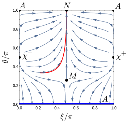
Figure 3: RG flows (blue arrows) demonstrate the simultaneous existence of the stable fixed line (blue line) at point A and stable point N, depending on the initial conditions $(\xi,\theta)$ for electron interaction $g=0.72$ ($K=0.4$). Red line corresponds to the RG flow plotted in terms of the conductances in Fig. 4b.

The whole plane $(\theta,\xi)$ is divided into two regions in Fig. 3, depending on the interaction strength. One region corresponds to a basin of attraction to the point $N$, the other to the point $A$. The situation is similar to purely tunneling case (PTC) for symmetric non-chiral $Y$-junction Aristov et al. (2010). It was shown there that for PTC the points $A$ or $N$ are stable and separated by the unstable $M$ point. Any deviation from PTC, which means the backscattering in the main wire, leads to an additional RG flow driving the junction to truly stable $N$ point while $A$ becomes of saddle point type. In our present model we have the chiral PTC junction, and any additional modification of $S$-matrix is forbidden due to topological character of edge state and the absence of backscattering in the main wire.

Notice that for vanishing interaction, $g$, the FPs $A$ and $M$ merge, and the basin of attraction for $A$ point vanish. More precisely, $A$ point becomes of saddle-point type in this limit and is stable only for parallel polarization of the tip, $\xi=0,\pi$. All RG trajectories in this limit obey the equation

$$\cos\xi\tan^{2}(\theta/2)=\mbox{const}.$$ (23)

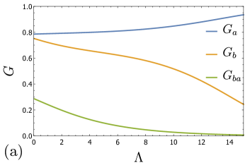
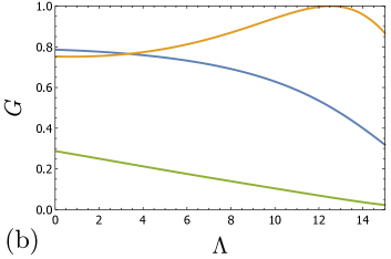
Figure 4: Full scaling curves for conductances are shown in panel (a) for electron interaction $g=0.47$ ($K=0.6$). The RG flow corresponds to going to the point $A$, i.e. effective detachment of the tip. The panel (b) shows the RG flows for stronger electron interaction $g=0.72$ ($K=0.4$). The conductances are renormalized to the point $N$, i.e. effective full breaking of the junction. Bare initial conductances on both panels are the same and the qualitative change in the RG flows is caused by the change in the interaction strength.

Since the position of $M$ point depends on the interaction strength, a qualitatively different behavior of renormalized conductances may occur even for their equal bare values at different interactions. Two examples of full scaling curves for conductances calculated for sizable interaction strength are shown in Fig. 4. The values of bare conductances are the same, but the panel (a) demonstrates RG flows going to the point $A$, whereas the panel (b) shows the system driven to the point $N$. This difference stems from the fact that changing interaction strength shifts the separating curve between the basins of attraction of the corresponding FPs.

IV Conclusions

We analyzed the simultaneous renormalization of asymmetry and total tunneling conductance from fully polarized tip into the helical edge state. In particular we showed that the RG flow for these two quantities is sensitive to the appearance of non-universal FP with asymmetry $\cos\xi_{M}=0$ and tunneling conductance $G_{b}\simeq\theta_{M}^{2}\simeq 2g$ for small interaction, $g$.

Our method assumes the existence of Fermi leads, which are needed for consistent definition of the S-matrix describing the Y-junction in terms of asymptotically free states. Experimentally it can be realized by the extended leads over the helical edge state. The helical edge state, on the other hand, is a topological object which cannot have disconnected ends. The dc current injected from the tunneling tip into the edge state may exit at another drain Y-junction. This implies the ring geometry with potentially important interference effects. The above picture of the renormalization of the single Y-junction should be valid when the temperature correlation length $\xi=v_{F}/T$ is smaller than the circumference of the edge state multiplied by $|r_{1}|^{2}$. The importance of interference effects is then reduced Dmitriev et al. (2010) but the corresponding analysis is beyond the scope of this study.

Appendix A Rotation of polarization axes

Our setup depicted in Fig. 1 is characterized by the angle $\xi$ between spin quantization axis in helical edge states and polarization direction in the tip. This junction is described by the $S$-matrix (2). We show that the two-parametric $S$ matrix can be obtained from one-parametric one by rotation of the edge states basis.

The Kramers spinor of scattered states is given by rearrangement of out- states, $\psi_{1,out}\leftrightarrow\psi_{2,out}$, by the matrix

$$F=\begin{pmatrix}0&1&0\\ 1&0&0\\ 0&0&1\end{pmatrix}.$$ (24)

The rotation of spin quantization axes is described by

$$U =\begin{pmatrix}e^{\frac{1}{2}i(\alpha+\gamma)}\cos\frac{\beta}{2}&e^{-\frac{1}{2}i(\alpha-\gamma)}\sin\frac{\beta}{2}&0\\ -e^{\frac{1}{2}i(\alpha-\gamma)}\sin\frac{\beta}{2}&e^{-\frac{1}{2}i(\alpha+\gamma)}\cos\frac{\beta}{2}&0\\ 0&0&1\end{pmatrix},$$ (25)

where the upper left 2$\times$2 matrix is $e^{i\gamma\sigma_{3}/2}e^{i\beta\sigma_{2}/2}e^{i\alpha\sigma_{3}/2}$ with $\alpha$, $\beta$, $\gamma$ are Euler angles and $\sigma_{2,3}$ Pauli matrices. For injected spin polarization parallel to the helical edge state, $\xi=0$, the form of $S$ matrix is simplified :

$$S_{\uparrow}=\begin{pmatrix}0&-\cos\theta&\sin\theta\\ -1&0&0\\ 0&\sin\theta&\cos\theta\end{pmatrix}.$$ (26)

If $\xi\neq 0(\pi)$ then we have to rotate the quantization basis of the helical edge states:

$$S=US_{\uparrow}FU^{\dagger}F.$$ (27)

The dependence of rotated $S$-matrix on angles $\alpha$ and $\gamma$ is removed by additional rephasing. The matrix (27) coincides with  (2) after the substitution $\beta\rightarrow-\xi$.

In our paper  Aristov and Niyazov (2016) the tunneling from the unpolarized tip into the helical edge states was discussed. This X junction was modeled by 4$\times$4 S matrix since there are two spin channels in unpolarized case. It was shown that a certain ratio of the conductances is not renormalized, see equation (26) in Aristov and Niyazov (2016). Applying the above arguments to the situation with X-junction, we confirm that the discussed ratio corresponds to the angle between the quantization axes for helical edge states and the tip (the quantity $-2\gamma$ in Aristov and Niyazov (2016) is the above Euler angle $\beta$). This observation clarifies the scale invariance of the ratio, as the choice for the spin quantization basis can be made arbitrarily without changing physical consequences.

The case of the corner X-junction between two helical edge states Aristov and Niyazov (2016) can also be discussed in terms of quantization axes rotation. Three stable FPs were obtained for repulsive interaction. One of them corresponds to the detachment of helical edge states independent of directions of the spin quantization axes. Two other FPs correspond to cases of parallel ($\beta=0$) or antiparallel ($\beta=\pi$) orientation of the quantization axes in individual edges. The choice between these FPs is defined by the value of relative orientation without interaction, $\beta<\pi/2$ or $\beta>\pi/2$, respectively.

Appendix B Ultraviolet cutoff 

The logarithmic corrections to conductance come from consideration of the interaction term, $g\int dx\,dy\,f(x-y)\rho(x)\tilde{\rho}(y)$, with the range function $f(x-y)$ of the screened Coulomb interaction having the property $\int dx\,f(x)=1$. In case of Luttinger model the interaction is point-like and $f(x-y)=\delta(x-y)$, which leads to the Hamiltonian (1). However this Luttinger form of interaction leads to ultraviolet divergence which is eventually cut off by another model assumption, formulated in the first line of Eq. (1) in the main text, namely, the absence of interaction in the vicinity of the junction on the scale $\ell$. We show now that the latter model assumption is not necessary if one assumes the finite range of the interaction, $r_{0}$.

To see it, we recall that the logarithmic type of integral (in the linear response) corresponds to the loop integration of the Green’s function $\delta I=\int_{0}^{\infty}d\omega\int_{0}^{L}dx\,dy\,f(x-y)\sin\omega(y+x)$, see Eq. (19) in Ref. Aristov and Wölfle (2014). Evaluating this integral we have

$$\delta I \simeq\tfrac{1}{2}\int_{0}^{\infty}d\omega\int_{-\infty}^{\infty}dr\,f(r)\int_{|r|}^{2L}dR\,\sin\omega R$$ (28)

$$\simeq\int_{0}^{\infty}\frac{d\omega}{2\omega}\int_{-\infty}^{\infty}dr\,f(r)(\cos\omega r-\cos 2\omega L)$$

It is clear that the finite range of interaction, $r_{0}$, becomes important in the limit of large $\omega\gtrsim r_{0}^{-1}$, cutting off the logarithmic divergence. Therefore $r_{0}$ plays the same role as the model scale $\ell$ and for our purposes we can take the larger of them as the ultraviolet scale of the theory.

Appendix C Fixed point $A$

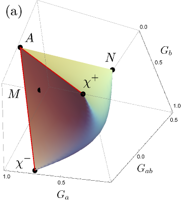
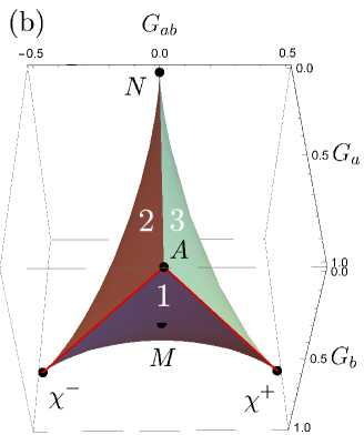
Figure 5: 2D fixed surface of physical conductances (7) in 3D conductances space is shown. Fixed points are depicted by black dots. Fixed lines corresponding to $\xi=0$, $\theta\in(0,\pi)$ and $\xi=\pi$, $\theta\in(0,\pi)$ are shown in red. The panel (b) shows that three domains near the point A are separated by ridges, which cannot be crossed by any RG flow. This explains why the point $A$ is stable for repulsive electron interaction in the domain 1 ( $\theta\approx 0$ ), and at the same time unstable in domains 2 and 3 ($\theta\approx\pi$, $\xi\approx 0(\pi)$).

Renormalization group (RG) analysis of the conductances (7) was performed in terms of parameters $\theta$ and $\xi$ because the RG equations are more transparent in this form. However, one may ask why the same point $A$ described as $\theta=0$ is stable and at the same time unstable when parametrized by $\theta=0$, $\xi=0(\pi)$. This situation is clarified by considering the surface of conductances in Fig. 5. It is seen that domains of different character (stable and unstable) near the point $A$ are separated by three ridges. Two of them are the lines $\xi=0$, $\theta\in(0,\pi)$ and $\xi=\pi$, $\theta\in(0,\pi)$ depicted by the red lines on the conductances surface, the third ridge connects $A$ and $N$ points. The domain 1 corresponds to $\theta\approx 0$ and the domain 2 (3) corresponds to $\theta\approx\pi$ but $\xi\approx 0(\pi)$. All these ridges are RG fixed lines, and any RG flow starting on these lines continues along them. It also means that any RG flow cannot pass across these ridges.

For completeness we provide here the scaling exponents at the FPs $A$ and $N$. The scaling exponent for the point $A$ depends on the direction of approach to this FP as explained above. In the domain 1 in Fig. 5 i.e. at $\theta\simeq 0$ we have only one scaling exponent for $\theta$, equal to $(1-K)^{2}/4K$. In the domains 2 and 3 in Fig. 5, i.e. at the points $\theta=\pi$, $\xi=0(\pi)$ we have additional scaling exponent, the RG flows away from $A$ point along $\xi$ with a weak impurity exponent $(1-K)$. Near the stable $N$ point the exponents along $\theta$ and $\xi$ are $\tfrac{1}{2}(K^{-1}-1)$ and $(K^{-1}-1)$.

References

- Hasan and Kane (2010) M. Z. Hasan and C. L. Kane, Rev. Mod. Phys. 82, 3045 (2010).
- Qi and Zhang (2011) X.-L. Qi and S.-C. Zhang, Rev. Mod. Phys. 83, 1057 (2011).
- Giamarchi (2004) T. Giamarchi, Quantum Physics in One Dimension, vol. 121 of The international series of monographs on physics (Clarendon; Oxford University Press, 2004), illustrated edition.
- Braunecker et al. (2012) B. Braunecker, C. Bena, and P. Simon, Phys. Rev. B 85, 021017 (2012).
- Kharitonov (2012) M. Kharitonov, Phys. Rev. B 86, 165121 (2012).
- Soori et al. (2012) A. Soori, S. Das, and S. Rao, Phys. Rev. B 86, 125312 (2012).
- Dolcetto et al. (2013a) G. Dolcetto, F. Cavaliere, D. Ferraro, and M. Sassetti, Phys. Rev. B 87, 085425 (2013a).
- Calzona et al. (2015a) A. Calzona, M. Carrega, G. Dolcetto, and M. Sassetti, Phys. Rev. B 92, 195414 (2015a).
- Calzona et al. (2016) A. Calzona, M. Acciai, M. Carrega, F. Cavaliere, and M. Sassetti, Phys. Rev. B 94, 035404 (2016).
- Chao et al. (2013) S.-P. Chao, S. A. Silotri, and C.-H. Chung, Phys. Rev. B 88, 085109 (2013).
- Dolcetto et al. (2013b) G. Dolcetto, N. T. Ziani, M. Biggio, F. Cavaliere, and M. Sassetti, physica status solidi (RRL) - Rapid Research Letters 7, 1059 (2013b).
- Steinberg et al. (2007) H. Steinberg, G. Barak, A. Yacoby, L. N. Pfeiffer, K. W. West, B. I. Halperin, and K. L. Hur, Nat Phys 4, 116 (2007).
- Hur et al. (2008) K. L. Hur, B. I. Halperin, and A. Yacoby, Annals of Physics 323, 3037 (2008).
- Pugnetti et al. (2009) S. Pugnetti, F. Dolcini, D. Bercioux, and H. Grabert, Phys. Rev. B 79, 035121 (2009).
- Das and Rao (2011) S. Das and S. Rao, Phys. Rev. Lett. 106, 236403 (2011).
- Garate and Le Hur (2012) I. Garate and K. Le Hur, Phys. Rev. B 85, 195465 (2012).
- Khanna et al. (2013) U. Khanna, S. Pradhan, and S. Rao, Phys. Rev. B 87, 245411 (2013).
- Calzona et al. (2015b) A. Calzona, M. Carrega, G. Dolcetto, and M. Sassetti, Physica E: Low-dimensional Systems and Nanostructures 74, 630 (2015b), ISSN 1386-9477.
- Santos et al. (2016) R. A. Santos, D. B. Gutman, and S. T. Carr, Phys. Rev. B 93, 235436 (2016).
- Kim et al. (2014) S. H. Kim, K.-H. Jin, J. Park, J. S. Kim, S.-H. Jhi, T.-H. Kim, and H. W. Yeom, Physical Review B 89, 155436 (2014).
- Li et al. (2015) T. Li, P. Wang, H. Fu, L. Du, K. A. Schreiber, X. Mu, X. Liu, G. Sullivan, G. A. Csáthy, X. Lin, et al., Phys. Rev. Lett. 115, 136804 (2015).
- Pauly et al. (2015) C. Pauly, B. Rasche, K. Koepernik, M. Liebmann, M. Pratzer, M. Richter, J. Kellner, M. Eschbach, B. Kaufmann, L. Plucinski, et al., Nat Phys 11, 338 (2015), ISSN 1745-2473.
- Wu et al. (2016) R. Wu, J.-Z. Ma, S.-M. Nie, L.-X. Zhao, X. Huang, J.-X. Yin, B.-B. Fu, P. Richard, G.-F. Chen, Z. Fang, et al., Phys. Rev. X 6, 021017 (2016).
- Giamarchi and Schulz (1988) T. Giamarchi and H. J. Schulz, Phys. Rev. B 37, 325 (1988).
- Furusaki and Nagaosa (1993) A. Furusaki and N. Nagaosa, Phys. Rev. B 47, 4631 (1993).
- Kane and Fisher (1992) C. L. Kane and M. P. A. Fisher, Phys. Rev. B 46, 15233 (1992).
- Matveev et al. (1993) K. A. Matveev, D. Yue, and L. I. Glazman, Phys. Rev. Lett. 71, 3351 (1993).
- Yue et al. (1994) D. Yue, L. I. Glazman, and K. A. Matveev, Phys. Rev. B 49, 1966 (1994).
- Oshikawa et al. (2006) M. Oshikawa, C. Chamon, and I. Affleck, Journal of Statistical Mechanics: Theory and Experiment 2006, P02008 (2006).
- Hou et al. (2012) C.-Y. Hou, A. Rahmani, A. E. Feiguin, and C. Chamon, Phys. Rev. B 86, 075451 (2012).
- Hou et al. (2009) C.-Y. Hou, E.-A. Kim, and C. Chamon, Phys. Rev. Lett. 102, 076602 (2009).
- Teo and Kane (2009) J. C. Y. Teo and C. L. Kane, Phys. Rev. B 79, 235321 (2009).
- Ström and Johannesson (2009) A. Ström and H. Johannesson, Phys. Rev. Lett. 102, 096806 (2009).
- Lal et al. (2002) S. Lal, S. Rao, and D. Sen, Phys. Rev. B 66, 165327 (2002).
- Das et al. (2004) S. Das, S. Rao, and D. Sen, Phys. Rev. B 70, 085318 (2004).
- Aristov and Wölfle (2009) D. N. Aristov and P. Wölfle, Phys. Rev. B 80, 045109 (2009).
- Aristov (2011) D. N. Aristov, Phys. Rev. B 83, 115446 (2011).
- Aristov and Wölfle (2012a) D. N. Aristov and P. Wölfle, Phys. Rev. B 86, 035137 (2012a).
- Aristov and Wölfle (2013) D. N. Aristov and P. Wölfle, Phys. Rev. B 88, 075131 (2013).
- Aristov and Wölfle (2012b) D. N. Aristov and P. Wölfle, Lithuanian Journal of Physics 52, 89 (2012b).
- Aristov and Niyazov (2016) D. N. Aristov and R. A. Niyazov, Phys. Rev. B 94, 035429 (2016).
- Aristov et al. (2010) D. N. Aristov, A. P. Dmitriev, I. V. Gornyi, V. Y. Kachorovskii, D. G. Polyakov, and P. Wölfle, Phys. Rev. Lett. 105, 266404 (2010).
- Aristov and Wölfle (2011) D. N. Aristov and P. Wölfle, Phys. Rev. B 84, 155426 (2011).
- Dmitriev et al. (2010) A. P. Dmitriev, I. V. Gornyi, V. Y. Kachorovskii, and D. G. Polyakov, Phys. Rev. Lett. 105, 036402 (2010).
- Aristov and Wölfle (2014) D. N. Aristov and P. Wölfle, Phys. Rev. B 90, 245414 (2014).