1in.9in.5in1.1in

Counterfactual Prediction with

Deep Instrumental Variables Networks

Jason Hartford, University of British Columbia

Greg Lewis, Microsoft Research and NBER

Kevin Leyton-Brown, University of British Columbia

Matt Taddy, Microsoft Research and the University of Chicago

We are in the middle of a remarkable rise in the use and capability of artificial intelligence. Much of this growth has been fueled by the success of deep learning architectures: models that map from observables to outputs via multiple layers of latent representations. These deep learning algorithms are effective tools for unstructured prediction, and they can be combined in AI systems to solve complex automated reasoning problems. This paper provides a recipe for combining ML algorithms to solve for causal effects in the presence of instrumental variables – sources of treatment randomization that are conditionally independent from the response. We show that a flexible IV specification resolves into two prediction tasks that can be solved with deep neural nets: a first-stage network for treatment prediction and a second-stage network whose loss function involves integration over the conditional treatment distribution. This Deep IV framework imposes some specific structure on the stochastic gradient descent routine used for training, but it is general enough that we can take advantage of off-the-shelf ML capabilities and avoid extensive algorithm customization. We outline how to obtain out-of-sample causal validation in order to avoid over-fit. We also introduce schemes for both Bayesian and frequentist inference: the former via a novel adaptation of dropout training, and the latter via a data splitting routine.

1 Introduction

Supervised machine learning (ML) provides a myriad of effective methods for solving prediction tasks. In these tasks, the learning algorithm is trained and validated to do a good job predicting the outcome for future examples from the same data generating process (DGP). However, decision makers (and automated decision systems) look to the data to model the effects of a policy change. Precisely because policy is going to change, the future relationship between inputs and outcomes will be different from what is in the training data. The ML algorithm will do a poor job of predicting the many potential futures associated with each policy option.

For example, optimal pricing requires predicting sales under changes to prices, a doctor needs to know how a patient will respond to various treatment options, and advertisers want to identify ads that cause sales. In order to accurately answer such counterfactual questions it is necessary to model the structural (or causal) relationship between policy (i.e., treatment) and outcome variables. Randomized control (‘AB’) trials are the gold standard for establishing causal relationships, but conducting them is often impractical or excessively expensive. Observational data, by contrast, is abundant. This paper uses the concept of instrumental variables to construct systems of machine learning (ML) tasks that can be applied in causal inference. We develop recipes for application of deep neural nets (DNNs) within these systems, with the result that we are able to leverage supervised ML to establish causal relationships in large and unstructured datasets.

The instrumental variables (IV) framework is a general class of methods for using observational data to establish causal relationships. It has a long history, especially in economics [e.g., Wright, 1928, Reiersøl., 1945]. The idea is to use sets of variables that only affect treatment assignment and not the outcome variable—so-called instruments—to consistently estimate the causal treatment effect. The framework is most straightforward in the case of an imperfect experiment. Consider a scenario where one of the inputs to treatment assignment has been randomized, but where other influences are potentially endogenous: they are connected to unobserved influences on the outcome. For example, in a medical trial we might have a treatment that is made available to a random sample of patients. However, only a portion of those patients actually take the treatment (perhaps because it causes discomfort). In this scenario, the random availability of treatment is our instrument and an IV analysis is used to infer the causal treatment effect in the face of selective partial adherence.

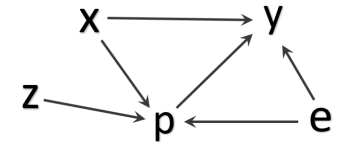
The full scope of IV analysis comes from its use in so-called natural experiments, where the instruments are contained in observational data and are not the result of intentional randomization. For example, a policy-maker might want to understand consumer price sensitivity to airfare (e.g., in setting an ‘airport improvement fee’): they need to model the effect of price (treatment) on sales (outcome). Prices vary for many reasons, some of them driven by demand. Regression of price on sales will fail to capture the true causal relationship: prices are high around holidays because demand is high and naive analysis will say that higher prices lead to more sales (nonsense). The problem is existence of factors that lead to co-movement in price and demand. Some of these are observable, such as major holidays, but many will be unknown to the policy-maker (on-line search activity, route capacity, etc). However, you could argue that cost of fuel is an instrument: it varies for reasons independent of demand and affects sales only via ticket prices. We can thus understand the causal effect of price on sales by observing how demand varies with the cost of fuel. Changes in fuel cost create movement in ticket prices that is independent of unobserved demand shifts, and this movement is as good as randomization for the purposes of causal inference. See Figure 1 for a graphical illustration of this scenario.

Figure 1: A graphical model showing a simple version of the structure of the observational DGP under our IV specification. In addition, we will assume that $e$ influences $y$ as an additive effect. On the right, we give names to the variables in the context of our simple air-travel demand example. Price is the policy variable, sales is the outcome, and there are (say) business- and leisure-travel customer types as observable covariates. There is a big ‘conference’, unobserved to the policy-maker, that drives demand and (due to the airline’s pricing algorithms) price. The instrument is the cost of fuel, which influences sales only via price.

Most IV applications make use of a two-stage least squares procedure [2SLS; e.g., Angrist et al., 1996] that requires assumptions of linearity and homogeneity (e.g., all airline customers must have the same price sensitivity). Nonparametric IV methods from the econometrics literature relax these assumptions [e.g., Newey and Powell, 2003]. However, these methods work by modeling the outcome as an unknown linear combination of a pre-specified set of basis functions of the treatment and other covariates (e.g. Hermite polynomials, wavelets or splines) and then modeling the conditional expectation of each of these basis functions in terms of the instruments (i.e. the number of equations is quadratic in the number of basis functions). This requires a strong prior understanding of the DGP by the researcher, and the complexity of both specification and estimation explodes when there are more than a handful of inputs.

Advances in deep learning have demonstrated the effectiveness for prediction tasks of learning latent representations of complex features spaces [for recent surveys, see LeCun et al., 2015, Schmidhuber, 2015]. We want to use these powerful learning algorithms for IV analysis. We do this by deriving from the IV structure a system of machine learning tasks that can each be targeted with deep learning and which, when solved, allow us to make counterfactual claims and perform causal inference. We break IV analysis into two ML stages: a first stage that models the conditional distribution for treatment given the instruments and covariates, and a second stage which targets a loss function involving integration over the conditional treatment distribution from the first stage. Both stages are use deep neural nets trained via stochastic gradient descent [Robbins and Monro, 1951, Bottou, 2010] and out-of-sample causal validation guards against over-fit. We refer to this setup as the Deep IV framework.

We highlight the main contributions to the ML and AI literatures.

Economic AI: This work uses econometric theory to resolve economic measurement questions into prediction tasks that can be targeted with deep learning algorithms. It is among the first examples of such a strategy, building from an earlier literature that combines ML with econometrics, e.g., for sparse linear models in Belloni et al. [2012, 2014] and for trees and forests in Athey and Imbens [2016], Wager and Athey [2015]. Our approach is designed to take advantage of generic ML capabilities and avoid extensive algorithm customization. This allows state-of-the-art DNN architectures to be plugged into economically relevant systems, and we hope that it will lead more ML researchers to target their efforts towards solving problems in this important domain. In our specific applications, this strategy lets us infer user- and time-specific treatment effects from complicated data involving raw text, images, and detailed hierarchical information.

Causal Validation: In a standard predictive ML setting, out-of-sample (OOS) validation is essential for setting tuning parameters and avoiding over-fit. Simple schemes, such as cross validation, do not work for causal inference because the available data is not immediately representative of the potential counterfactual outcomes. However, our framework resolves causal inference into two prediction problems and we show how our fit for each of these tasks can be evaluated on left-out data. This provides a general approach to model tuning and validation for causal inference.

Integral SGD: The second stage of our Deep IV framework involves training a DNN whose role in the loss function is integrated over a distribution of possible inputs. In our case, the integral is with respect to the conditional treatment distribution; however, similar setups show up elsewhere in ML [e.g., the variational autoencoders of Kingma and Welling, 2013]. We specify how SGD should be applied when these integrals are high-dimensional and need to be solved via Monte Carlo (MC) sampling: independent samples should be used for each instance of the integral in a gradient calculation, and it is most efficient to use a single MC draw for each gradient observation. These results will be generally applicable for learning algorithms that entail integral loss functions.

Inference: We provide techniques for both Bayesian and frequentist inference about the treatment effects. In the first case, we show that a network trained under dropout [Srivastava et al., 2014] can be interpreted as a very simple form of variational Bayesian inference with a posterior precision that is fixed by the dropout rate. This provides a more direct and interpretable connection between dropout and Bayesian inference than that derived in Gal and Ghahramani [2015] (it also offers guidance on how to choose the dropout rate). In the second case, we use a sample-splitting strategy that allows us to study the fitted network structure, and its implications for treatment effects, via two-stage least-squares inference with left-out data.

Section 2 describes our general IV specification and its resolution into two ML tasks, while Section 3 outlines neural network estimation for these tasks with particular attention on the SGD routine used in model training. Section 4 then details both Bayesian and frequentist inference results and Section 5 provides simulation experiments to illustrate our methods.

2 Machine learning for counterfactual prediction

Consider the following structural equation with additive latent errors,

$$y=~{}\mathscr{g}(p,x)+e,$$ (1)

where $y$ is the outcome variable (e.g., sales in our airline example), $p$ is the policy or treatment variable (e.g., price), and $x$ is a vector of observable covariate features (e.g., time and customer characteristics). The function $~{}\mathscr{g}(\cdot)$ is some unknown and potentially non-linear continuous function of $x$ and $p$, and the ‘unobservable’ error $e$ enters additively with unconditional mean $\operatorname*{\mathds{E}}e=0$. We emphasize that, in contrast to the usual machine learning setup, here the errors are potentially correlated with the inputs: $\mathds{E}[e|x,p]\neq 0$ and, in particular, $\mathds{E}[pe|x]\neq 0$. That is to say, the policy variable $p$ is endogenous.

Define the counterfactual prediction function

$$\mathscr{h}(p,x)\equiv~{}\mathscr{g}(p,x)+\operatorname*{\mathds{E}}[e|x],$$ (2)

which is the conditional expectation of $y$ given the observables $p$ and $x$, holding the distribution of $e$ constant as $p$ is changed. Note that we condition only on $x$ and not $p$ in the term $E[e|x]$; this term is typically nonzero, but it will remain constant under arbitrary policy changes. Thus $\mathscr{h}(p,x)$ is the structural estimand of interest; to evaluate policy options, say $p_{0}$ and $p_{1}$, we can look at the difference in mean outcomes $\mathscr{h}(p_{1},x)-\mathscr{h}(p_{0},x)=~{}\mathscr{g}(p_{1},x)-~{}\mathscr{g}(p_{0},x)$.

In standard ‘unstructured’ ML, the prediction model is trained to fit $\operatorname*{\mathds{E}}[y|p,x]$. This estimand will typically be biased against our structural objective:

$$\operatorname*{\mathds{E}}[y|p,x]=~{}\mathscr{g}(p,x)+\operatorname*{\mathds{E}}[e|p,x]\neq\mathscr{h}(p,x)$$ (3)

since presence of error endogeneity – $\mathds{E}[pe|x]\neq 0$ – implies that $\operatorname*{\mathds{E}}[e|p,x]\neq\operatorname*{\mathds{E}}[e|x]$. Endogeneity occurs whenever unobservables are correlated with both policy and outcome, as was the case for price and sales in our demand example. This object is inappropriate for policy analysis as it will lead to biased counterfactuals:

$$\operatorname*{\mathds{E}}[y|p_{1},x]-\operatorname*{\mathds{E}}[y|p_{0},x]=~{}\mathscr{g}(p_{1},x)-~{}\mathscr{g}(p_{0},x)+\left(\operatorname*{\mathds{E}}[e|p_{1},x]-\operatorname*{\mathds{E}}[e|p_{0},x]\right).$$ (4)

Fortunately, the presence of instruments allows us to estimate an unbiased ${\hat{\mathscr{h}\mkern 4.0mu}\mkern-4.0mu}{}(p,x)$ that captures the structural relationship between $p$ and $y$. These are variables, say $z$, that satisfy three conditions:

• Relevance: $F(p|x,z)$, the distribution of $p$ given $x$ and $z$, is not constant in $z$,

• Exclusion: z does not enter equation (1) – i.e., $z\perp\!\!\!\!\!\perp y\;|\;(x,p,e)$,

• Unconfounded Instrument: $z$ is conditionally independent of the error – i.e., $z\perp\!\!\!\!\!\perp e\;|\;x$.

The last condition is chosen to match the ‘unconfoundedness’ assumption in the Neyman-Rubin potential outcomes framework [Rosenbaum and Rubin, 1983] (i.e. $p\perp\!\!\!\!\!\perp e\;|\;x$). But our assumption is weaker — in particular, we allow for $p\not\perp\!\!\!\!\!\perp e|x$ — and so the matching and propensity-score re-weighting approaches often used in that literature will not work here. Figure 1 presents a graphical model summarizing a simple IV system.

Taking the expectation of both sides of (1) conditional on $[x,z]$ and applying these assumptions establishes the relationship [cf. Newey and Powell, 2003]:

$$\operatorname*{\mathds{E}}[y|x,z]~{}=~{}\operatorname*{\mathds{E}}[~{}\mathscr{g}(p,x)|x,z]+\operatorname*{\mathds{E}}[e|x]~{}=~{}\int\mathscr{h}(p,x)dF(p|x,z)$$ (5)

where, again, $dF(p|x,z)$ is the conditional treatment distribution. This shows that we can reason about our counterfactual prediction function $\mathscr{h}(p,x)$ (the RHS of (5)) by learning to predict $\operatorname*{\mathds{E}}[y|x,z]$ (the LHS of (5)). The relationship in (5) defines an inverse problem for $\mathscr{h}$ in terms of two directly observable functions: $\mathds{E}[y|x,z]$ and $F(p|X,z)$. Specifically, to minimize $\ell_{2}$ loss given $T$ data points and given a function space $\mathcal{H}$ (which may not include the true $\mathscr{h}$), we solve

$$\min_{{\hat{\mathscr{h}\mkern 4.0mu}\mkern-4.0mu}{}\in\mathcal{H}}\sum_{t=1}^{T}\left(y_{t}-\int{\hat{\mathscr{h}\mkern 4.0mu}\mkern-4.0mu}{}(p,x)dF(p|x_{t},z_{t})\right)^{2}.$$ (6)

Since the treatment distribution is unknown, IV analysis typically splits into two stages: a first to estimate $\hat{F}(p|x_{t},z_{t})\approx F(p|x_{t},z_{t})$, and a second to minimize (6) after replacing $F$ with $\hat{F}$.

Existing approaches to IV analysis rely upon a linearization of both ${\hat{\mathscr{h}\mkern 4.0mu}\mkern-4.0mu}{}$ and $\hat{F}$. For example, the popular two-stage least-squares (2SLS) procedure posits

$$y =\gamma p+x\beta_{y}+e,$$ (7)

$$p =\tau z+x\beta_{p}+v$$

with the assumptions that $E[e|x,z]=0$, $E[v|x,z]=0$ and $E[ev]\neq 0$ (which implies $E[ep]\neq 0$). In this case, the integral in (6) simplifies as

$$\int{\hat{\mathscr{h}\mkern 4.0mu}\mkern-4.0mu}{}(p,x)dF(p|x,z)=\gamma\operatorname*{\mathds{E}}[p|x,z]+x\beta_{y}+\operatorname*{\mathds{E}}[e|x]=\gamma(\tau z+x\beta_{p})+x\beta_{y},$$

The 2SLS approach is to replace the unknown $\operatorname*{\mathds{E}}[p|x,z]$ with an estimate $\hat{}p=\hat{\tau}z+x\hat{\beta}_{p}$. In the ‘first-stage’ $\hat{}p$ is estimated by an ordinary least squares (OLS) regression of $p$ on $x$ and $z$. You then run a ‘second-stage’ regression of $y=\gamma\hat{}p+x\beta_{y}$, again by OLS.

The 2SLS procedure is a straightforward and statistically efficient way to estimate the effect of the policy variable (i.e. $\gamma$), but requires two strong assumptions: linearity (i.e., that both first and second stage regressions are correctly specified) and homegeneity (i.e., that the policy affects all individuals in the same way). Flexible nonparametric extensions of 2SLS, such as in Newey and Powell [2003], replace the simple linear regressions in (7) with a linear projection onto a series of known basis functions. The outcome equation is replaced with $y=\sum_{k}\gamma_{k}\varphi_{k}(p,x)+e$, where $\varphi_{k}$ are pre-specified functions and the conditional expectation $\operatorname*{\mathds{E}}[\varphi_{k}(p,x)|x,z]$ of each of these bases is estimated in a series of non-parametric first stage regressions. The non-parametric first stage estimators are often series estimators, and so require another basis expansion (now in $[x,z]$). Thus, although this is an effective strategy for introducing flexibility and heterogeneity with low dimensional inputs, this system of series estimators becomes computationally intractable for anything beyond trivially low-dimensional $[x,z]$.

This paper proposes to avoid explicit linearization by instead directly targeting the integral objective in (6). In the case where $p$ is low dimensional, we replace the integral with a sum over its support. When this is not feasible, we use efficient Monte Carlo integration inside a stochastic gradient descent routine. In either case, $F$ and $\mathscr{h}$ can be learned by any generic ML model that can be trained via gradient descent. We make use of deep neural networks, allowing us to take advantage of state-of-the-art ML technology, and provide a recipe for two-stage deep learning. The next section details these ideas and their implementation.

3 Estimation and neural network implementation

As mentioned, our approach proceeds in two stages. We outline each in-turn before discussing Monte Carlo SGD for our second-stage objective and a framework for out-of-sample validation.

3.1 First stage: Treatment network

In the first stage we learn $F(p|x,z)$ using an appropriately chosen distribution parameterized by a DNN, say $\hat{F}=F_{\phi}(p|x,z)$ where $\phi$ is the set of network parameters. Since we will be integrating over $F_{\phi}$ in the second stage, we must fully specify this distribution. Estimation then proceeds by maximum likelihood via SGD on the implied negative log likelihood.

In the case of discrete $p$, we model $F_{\phi}(p|x,z)$ as a multinomial $\mathrm{MN}\left(p\mid\pi(x,z;\phi)\right)$ with $\mathrm{p}(p=p^{k})=\pi_{k}(x,z;\phi)$ for each treatment category $p^{k}$ and where $\pi_{k}(x,z;\phi)$ is given by a DNN with softmax output. For continuous treatment, we model $F$ as a mixture of Gaussian distributions

$$F_{\phi}(p|x,z)=\sum_{k}\pi_{k}(x,z;\phi)\mathrm{N}\left(\mu_{k}(x,z;\phi),\sigma^{2}_{k}(x,z;\phi)\right),$$

where component weights $\pi_{k}(x,z;\theta)$ and parameters $\left[\mu_{k}(x,z;\phi),\sigma_{k}(x,z;\phi)\right]$ form the final layer of a neural network parametrized by $\phi$. This model is known as a mixture density network, as detailed in §5.6 of Bishop [2006]. With enough mixture components it can approximate arbitrary smooth densities. Mixed continuous-discrete distributions are obtained by replacing some mixture components with a point mass. In each case, fitting $F_{\phi}$ is a standard ML task.

3.2 Second stage: Outcome network

In the second stage, our counterfactual prediction function $\mathscr{h}$ is approximated by a DNN with real-valued output, say $\mathscr{h}_{\theta}$. Following from (6), network parameters $\theta$ are optimized to minimize the integral loss function, over training data $D$ of size $T=|D|$ from the joint DGP $\mathcal{D}$,

$$\mathcal{L}(D;\theta)=|D|^{-1}\sum_{t}\left(y_{t}-\int\mathscr{h}_{\theta}(p,x_{t})dF_{\phi}(p|x_{t},z_{t})\right)^{2}.$$ (8)

Note that this loss involves the estimated treatment distribution function, $F_{\phi}$, from our first stage.

We use stochastic gradient descent [SGD; see specific algorithms in, e.g., Duchi et al., 2011, Kingma and Ba, 2014] to train the network weights. For $F_{\phi}$, standard off-the-shelf methods apply. Our second stage optimization, for $\mathscr{h}_{\theta}$, needs to account for the integral in (8). The noisy SGD sample gradient, for a single observation $d_{t}=[x_{t},z_{t},p_{t},y_{t}]$, is available as

$$\nabla_{\theta}\mathcal{L}_{t}\equiv\frac{\partial\mathcal{L}(d_{t};\theta)}{\partial\theta}=\left(y_{t}-\int\mathscr{h}_{\theta}(p,x_{t})dF_{\phi}(p|x_{t},z_{t})\right)\int\mathscr{h}_{\theta}^{\prime}(p,x_{t})dF_{\phi}(p|x_{t},z_{t}),$$ (9)

assuming continuity of both $\mathscr{h}_{\theta}$ and $\mathscr{h}_{\theta}^{\prime}$, where $\mathscr{h}_{\theta}^{\prime}=\partial\mathscr{h}_{\theta}/\partial\theta$. When the policy space is discrete and low dimensional, in which case Section 3.1 specifies a multinomial response network for $F_{\phi}$, this gradient can be expressed exactly as

$$\nabla_{\theta}\mathcal{L}_{t}=-2\left(y_{t}-\sum_{k}\pi_{k}(x_{t},z_{t};\phi)\mathscr{h}_{\theta}(p^{k},x_{t})\right)\sum_{k}\pi_{k}(x_{t},z_{t};\phi)\mathscr{h}_{\theta}^{\prime}(p^{k},x_{t}).$$ (10)

For more complicated and continuous treatments, the integrals must be approximated. The next section proposes an efficient Monte Carlo approximation SGD algorithm.

3.3 SGD with Monte Carlo integration

SGD convergence requires that each sampled gradient $\nabla_{\theta}\mathcal{L}_{t}$ is unbiased for the population gradient, $\nabla_{\theta}\mathcal{L}(\mathcal{D};\theta)$. Lower variance for $\nabla_{\theta}\mathcal{L}_{t}$ will tend to yield faster convergence [Zinkevich, 2003] while the computational efficiency of SGD on large datasets requires limiting the number of operations going into each gradient calculation [Bousquet and Bottou, 2008]. We are thus free to replace the integrals in (9) with anything that leads to unbiased estimates of the complete gradient, and should do so to minimize variance under a constraint on the number of operations involved.

Basic Monte Carlo (MC) methods replace an integral with respect to a probability measure with the average of draws from the associated probability distribution: $\int\mathscr{h}(p)dF(p)=\operatorname*{\mathds{E}}_{F}\mathscr{h}(p)\approx B^{-1}\sum_{b}\mathscr{h}(p_{b})$ for $\{p_{b}\}_{1}^{B}\stackrel{{\scriptstyle iid}}{{\sim}}F$. This method can be applied in our context with an important caveat: independent samples must be used for each instance of the integral in the gradient calculation. To see this, note that (9) has expectation

$$\mathds{E}_{\mathcal{D}}\nabla_{\theta}\mathcal{L}_{t} =-2\mathds{E}_{\mathcal{D}}\left(\mathds{E}_{F_{\phi}(p|x_{t},z_{t})}\!\!\left[y_{t}-\mathscr{h}_{\theta}(p^{k},x_{t})\right]\mathds{E}_{F_{\phi}(p|x_{t},z_{t})}\!\!\left[\mathscr{h}_{\theta}^{\prime}(p^{k},x_{t})\right]\right)$$ (11)

$$\neq-2\mathds{E}_{\mathcal{D}}\mathds{E}_{F_{\phi}(p|x_{t},z_{t})}\!\!\left[\left(y_{t}-\mathscr{h}_{\theta}(p^{k},x_{t})\right)\mathscr{h}_{\theta}^{\prime}(p^{k},x_{t})\right],$$ (12)

where the inequality holds so long as $\mathrm{cov}_{F_{\phi}(p|x_{t},z_{t})}\!\!\left[\left(y_{t}-\mathscr{h}_{\theta}(p^{k},x_{t})\right)\mathscr{h}_{\theta}^{\prime}(p^{k},x_{t})\right]\neq 0$. We thus need a gradient estimate based on unbiased MC estimates for each $\mathds{E}_{F_{\phi}(p|x_{t},z_{t})}$ term in (11). This is obtained by taking two samples $\{\dot{p}_{b}\}_{1}^{B},\{\ddot{p}_{b}\}_{1}^{B}\stackrel{{\scriptstyle iid}}{{\sim}}F_{\phi}(p|x_{t},z_{t})$ and calculating the gradient as

$$\widehat{\nabla}_{\theta}^{B}\mathcal{L}_{t}\equiv-2\left(y_{t}-B^{-1}\sum_{b}\mathscr{h}_{\theta}(\dot{}p_{b},x_{t})\right)B^{-1}\sum_{b}\mathscr{h}_{\theta}^{\prime}(\ddot{}p_{b},x_{t}).$$ (13)

Independence of the two samples ensures that $\mathds{E}\widehat{\nabla}_{\theta}^{B}\mathcal{L}_{t}=\mathds{E}_{\mathcal{D}}\nabla_{\theta}\mathcal{L}_{t}=\nabla_{\theta}\mathcal{L}(\mathcal{D};\theta)$, as desired.

The estimator in (13) remains unbiased even in the case of $B=1$, where our gradient becomes

$$\widehat{\nabla}_{\theta}\mathcal{L}_{t}\equiv\widehat{\nabla}_{\theta}^{1}\mathcal{L}_{t}=-2\left(y_{t}-\mathscr{h}_{\theta}(\dot{}p,x_{t})\right)\mathscr{h}_{\theta}^{\prime}(\ddot{}p,x_{t}),~{}~{}~{}\dot{p},\ddot{p}\stackrel{{\scriptstyle iid}}{{\sim}}F_{\phi}(p|x_{t},z_{t}).$$ (14)

Indeed, this ‘two-draw’ $\widehat{\nabla}_{\theta}\mathcal{L}_{t}$ is the optimal implementation of (13) in a large-scale learning setting [Bousquet and Bottou, 2008] where computation, rather than the amount of data available, is the binding constraint on error minimization. Consider two alternative gradient estimators, both of which require roughly the same number of computational operations: $\widehat{\nabla}_{\theta}^{M}\mathcal{L}_{t}$ and $M^{-1}\sum_{m=1}^{M}\widehat{\nabla}_{\theta}\mathcal{L}_{t_{m}}$, where this latter term is just the average of $M$ two-draw gradients across unique data points. The variance of the first estimator is $M^{-1}\mathds{E}_{\mathcal{D}}\left[\mathrm{var}_{F_{\phi}(p|x,z)}(\widehat{\nabla}_{\theta}\mathcal{L}_{t})\right]+\mathrm{var}_{\mathcal{D}}\nabla_{\theta}\mathcal{L}_{t}$, which due to the second non-diminishing term will tend to be larger than $M^{-1}\mathrm{var}_{\mathcal{D}}\widehat{\nabla}_{\theta}\mathcal{L}_{t}$, the variance of the second estimator. Hence, efficient MC SGD will process more two-draw gradients $\widehat{\nabla}_{\theta}\mathcal{L}_{t}$ rather than spending time increasing the number of MC draws for a single sampled gradient.

As an aside, we note that this MC SGD algorithm – and the requirement of independent sampling for each integral – will apply to a wide range of loss functions that compose a norm and an integral. This includes any implementation of the variational auto-encoders of Kingma and Welling [2013] that involve, e.g., $\ell_{2}$ observation loss. In addition, there are a number of applications in economics and elsewhere that approach such loss functions through direct minimization of a monte carlo approximation to the true objective function (e.g., simulated maximum likelihood (SML) and simulated method of moments (SMM) [McFadden, 1989, Pakes and Pollard, 1989]). For example, in our case one would minimize the simulated objective $\sum_{t}\left(y_{t}-B^{-1}\sum_{b}\mathscr{h}_{\theta}(p^{b}_{t},x_{t})\right)^{2}$ for $\{p^{b}_{t}\}$ a sample of size $BT$ from $F_{\phi}(p|x_{t},z_{t})$, using an arbitrary minimization technique. The simulated objective must be uniformly close (as a function of the parameters) to the original objective to guarantee that the solutions are close. This requires $B$ large, which is computationally intensive and potentially prohibitive if $T$ is large. By contrast, our MC SGD scheme directly solves the original problem, and in a computationally efficient manner; it may thus be useful to economists in a large-data setting.

3.4 Causal validation

Any complex ML framework requires an out-of-sample (OOS) validation procedure for tuning hyperparameters and optimization rules. Fortunately, Deep IV can be validated with left-out data corresponding to each individual composite ML task.

Consider a left-out dataset $D_{lo}$. Our first stage, fitting $F_{\phi}$, is a standard density estimation problem and can be tuned to minimize the OOS deviance criterion

$$\min_{\phi}\sum_{d_{l}\in D_{lo}}-\log f_{\phi}(p_{l}|x_{l},z_{l}),$$ (15)

where $f_{\phi}$ is either the probability mass function or density function associated with $F_{\phi}$, as appropriate. Second stage validation proceeds conditional upon a fitted $F_{\phi}$, and we seek to minimize the left-out loss criterion

$$\min_{\theta}\sum_{d_{l}\in D_{lo}}\left(y_{l}-\int\mathscr{h}_{\theta}(p,x_{l})dF_{\phi}(p|x_{l},z_{l})\right)^{2}.$$ (16)

The integral here can either be exact or MC approximate via sampling from $F_{\phi}$.

Each stage is evaluated in turn, with second stage validation using the best-possible network as selected in the first stage. Statistical ‘overfit’ – optimizing to noise – will lead to a reduction in performance in each of these criteria. In the first stage, using (15) to avoid overfit guards against the ‘weak instruments’ bias [Bound et al., 1995] that can occur when the instruments are only weakly correlated with the policy variable. In the second stage, minimizing (16) will lead to best-possible performance on the objective $\mathds{E}[y|x,z]$ under the constraint imposed by $F_{\phi}$. Note that these criteria provide relative performance guidance: improving on each criterion will improve your performance on counterfactual prediction problems, but it does not tell you, e.g., how far $\mathscr{h}_{\theta}(p,x)$ is from true $\mathscr{h}(p,x)$. That requires the inference steps of the next section.

4 Inference

In many ML applications, inference and uncertainty quantification are of secondary importance after average predictive performance. However, in policy decision settings it is crucial to know the credibility and variance of our counterfactual predictions. This section addresses these needs.

4.1 Frequentist inference and statistical properties

Under the relevance, exclusion, and unconfoundedness conditions of Section 2, which define the role of instruments, nonparametric identification of the function $\mathscr{h}$, known to be an element of some function space $\mathcal{H}$, simply requires that there is a unique solution for $\mathscr{h}\in\mathcal{H}$ in equation (5): $\mathds{E}[y|x,z]=\int\mathscr{h}(p,x)dF(p|x,z)$. When $p$ and $z$ are discrete, it is necessary and sufficient that the Markov matrix describing the conditional distribution of $p$ given $z$ for fixed $x$ has full rank with probability 1 (where the measure is over the distribution of $x$) [Newey and Powell, 2003]. This says, roughly, that $z$ generates sufficient variation in $p$ for every $x$ that occurs with positive probability, which is necessary to identify heterogeneous treatment effects.

In practice, it is of primary importance to assess the validity of the structural IV conditions. Outside of some special scenarios [Pearl, 1995], exclusion and unconfoundedness are untestable and must be assumed. This is easy for randomized instruments (e.g., intent-to-treat), and there is extensive guidance in the economics literature for assessment of natural experiments [see Angrist and Pischke, 2008, for an introduction].

Relevance can be observed: when instruments are non-informative at some $x$, then $F(p|z,x)=F(p|x)$. The neural network will typically lead $F_{\phi}(p|z,x)$ to vary with $z$ when the instruments are unconditionally relevant, even at $x$ locations that see little instrument-treatment variation in the finite training sample. That is, we will be semi-parametrically identified due to variation at neighboring covariate locations. We can also consider what happens when the first stage yields irrelevance at a given $x$: the second stage then targets $\left(y-\int\mathscr{h}_{\theta}(p,x)dF_{\phi}(p|x)\right)^{2}$, which at a fixed $x$ implies $\mathscr{h}_{\theta}(p,x)=\mathscr{h}_{\theta}(x)=\mathds{E}[y|x]$, a constant. So where relevance fails the second stage objective pushes towards estimates of a zero policy effect.

If identification is satisfied, consistency of Deep IV follows from Newey and Powell [2003, Lemma A1 and Theorem 4.1] if we treat both $F_{\phi}$ and $\mathscr{h}_{\theta}$ as sieve estimators that grow in complexity so that they can arbitrarily closely approximate the true $F$ and $\mathscr{h}$. Unfortunately, full Frequentist inference results for $\mathscr{h}_{\theta}$, or for $\theta$, are not available via any reasonable asymptotic approximations. Instead, we turn to a data splitting procedure wherein some portion of the data is left-out of the training sample and used to obtain conditional inference for $\mathscr{h}_{\theta}$. Splitting procedures like this have a long history [Cox, 1975], and have recently regained popularity as an option for inference post model-selection [e.g., Fithian et al., 2015, Wager and Athey, 2015].

Denote the $K_{L}$ nodes in the final layer of the response network (i.e., $\mathscr{h}_{\theta}$) as $\eta_{k}(x,p)$, where the arguments $[x,p]$ are implictly fed through lower layers via weights $\theta$, and their conditional expectation at observation $i$ as

$$\bar{\eta}_{ik}=\mathds{E}_{F_{\phi}(p|x_{i},z_{i})}\eta_{k}(x_{i},p).$$ (17)

As always, this expectation can be evaluated either exactly for discrete $p$ or via MC approximation. Hence, the second stage network parameters, $\theta$, have been optimized to minimize $\sum_{d_{i}\in D}\left(y_{i}-\sum_{k}\bar{\eta}_{ik}\right)^{2}$ over the in-sample training data $D$. In addition, we introduce the shorthand $\eta_{ik}=\eta_{k}(x_{i},p_{i})$ for the node expressions at observed treatment values, and denote observation vectors as ${\eta}_{i}=[1~{}\eta_{i1}\cdots\eta_{iK_{L}}]^{\prime}$ and ${\bar{\eta}}_{i}=[1~{}\bar{\eta}_{i1}\cdots\bar{\eta}_{iK_{L}}]^{\prime}$.

Our data-splitting inference takes $\theta$ and $\phi$ as fixed after training and applies the fitted networks to calculate $\bar{\eta}_{lk}$ and $\eta_{lk}$ for left-out observations $d_{l}\in D_{lo}$. These values are then used as instruments and treatments, respectively, in standard linear IV estimation. Moreover, assuming homoskedastic errors, the instruments are the “right ones”: they are plug-in estimates of the infeasible optimal instruments, $E[\eta_{k}(x_{i},p)|x_{i},z_{i}]$ [Chamberlain, 1987].

Letting $T_{lo}=|D_{lo}|$, stack the left-out ‘data’ together as ${\bar{H}}=[{\bar{\eta}}_{1}\cdots{\bar{\eta}}_{T_{lo}}]^{\prime}$, ${H}=[{\eta}_{1}\cdots{\eta}_{T_{lo}}]^{\prime}$, and $Y=[y_{l}\cdots y_{T_{lo}}]^{\prime}$. Then, since there are exactly as many instruments as treatments, the 2SLS estimate for the causal effect of ${\eta}_{l}$ on $y_{l}$ can be written in its method of moments form as

$$\hat{\beta}=({\bar{H}}^{\prime}H)^{-1}{\bar{H}}^{\prime}Y.$$ (18)

Standard asymptotic arguments [e.g., Angrist and Pischke, 2008] give

$$V_{\beta}\equiv\mathrm{var}(\hat{\beta})=({\bar{H}}^{\prime}{\bar{H}})^{-1}{\bar{H}}^{\prime}\mathrm{diag}\left[({H}\hat{\beta}-Y)^{2}\right]{\bar{H}}({\bar{H}}^{\prime}{\bar{H}})^{-1}$$ (19)

as a consistent estimator for the sampling variance on $\hat{\beta}$. Note that (19) looks like the usual ‘sandwich’ variance estimator [White, 1980] for regression of $Y$ on ${\bar{H}}$, except that the sandwiched diagonal of squared residuals is calculated for the treatment input $H$ rather than for the instruments $\bar{H}$. Finally, defining ${\eta}(x,p)=[1~{}\eta_{1}(x,p)\cdots\eta_{K}(x,p)]^{\prime}$, the data-splitting estimate of our counterfactual prediction function $\mathscr{h}(x,p)$ is

$${\hat{\mathscr{h}\mkern 4.0mu}\mkern-4.0mu}{}(x,p)=\hat{\beta}^{\prime}{\eta}(x,p),$$ (20)

with sampling variance

$$\mathrm{var}\left({\hat{\mathscr{h}\mkern 4.0mu}\mkern-4.0mu}{}(x,p)\right)={\eta}^{\prime}(x,p)~{}V_{\beta}~{}{\eta}(x,p).$$ (21)

This ‘post selection’ variance might seem strange at first glance. Our data splitting procedure views the first and second stage network fits as a search over different candidate models for a good set of basis functions and their conditional expectations. The variance in (21) summarizes frequentist uncertainty conditional on that model. However, since we are calculating uncertainty out-of-sample, there is a surprising amount of information in $V_{\beta}$. For example, if the first stage does a poor job of modeling $F(p|x_{i},z_{i})$, then each $\bar{\eta}_{ik}$ will be far from $\eta(x_{i},p_{i})$ and the OLS residuals, $y_{i}-{\eta}_{i}^{\prime}\hat{\beta}$, will be large (driving up the variance in $V_{\beta}$). Moreover, Deep IV here can be viewed as automating the process of basis specification that authors such as Newey and Powell [2003], Blundell et al. [2007], and Chen and Pouzo [2012] execute by hand and treat as given.

4.2 Dropout variational Bayesian inference

For unconditional uncertainty quantification, we look to variational Bayesian inference. For each of our two networks, we fit a variational distribution that approximates the posterior distribution over network weights. In particular, we show that a network fit under dropout [Srivastava et al., 2014] parametrizes just such a variational distribution and thus approximate Bayesian inference requires no more work than dropout training (which is a good idea in any case).

We introduce the procedure in terms of a generic neural network before describing the extension to Deep IV. For simplicity we will ignore the network bias terms (i.e., the intercepts added to each layer input) in our description, but typically dropout is also applied to these terms. Define the $K_{l}\times K_{l-1}$ weight matrix from layer $l$ as $W_{l}$, where $K_{l}$ denotes the number of nodes in layer $l$. In dropout training, this matrix is parametrized as $W_{l}=\Xi_{l}\Omega_{l}$, where $\Omega_{l}$ is a fixed $K_{l}\times K_{l-1}$ matrix and $\Xi_{l}=\mathrm{diag}\left([\xi_{l1}\ldots\xi_{lK_{l}}]\right)$ with each $\xi_{kl}$ an independent $\mathrm{Bernoulli}(c)$ random variable where $\mathds{E}\xi_{kl}=c$. During training, each SGD update for $W_{l}$ follows gradients with respect to $\Omega_{l}$ conditional upon a random realization for $\Xi_{l}$; rows of $\Omega_{l}$ corresponding to zero draws of $\xi_{lk}$ are thus ‘dropped’ from the gradient calculations and updates.

Variational Bayesian inference [VB; e.g., Bishop, 2006] for parameters $W$ optimizes a parametric variational distribution, say $q(W)$, to be close to the true (but intractable) posterior density $\mathrm{p}(W|\mathcal{D})$. In particular, VB fits $q$ to minimize the Kullback-Leibler divergence $\mathds{E}_{q}\left[\log q(W)-\log\mathrm{p}(W|\mathcal{D})\right]$, which is equivalent to solving

$$\min_{q}\mathds{E}_{q}\left[~{}\log q(W)-\log\mathrm{p}(\mathcal{D}|W)-\log\mathrm{p}(W)~{}\right]$$ (22)

where $\mathrm{p}(\mathcal{D}|W)$ is the likelihood and $\mathrm{p}(W)$ is the prior. Say $W=\{W_{0}\ldots W_{L}\}$ is the full set of network weights across layers, and similarly for $\Omega$ and $\Xi$. Then we define our variational $q(W)$ as the distribution over weights induced by setting $W_{l}=\Xi_{l}\Omega_{l}$ with $\xi_{lk}\stackrel{{\scriptstyle iid}}{{\sim}}\mathrm{Bernoulli}(c)$. Writing $W_{lk}$ for the $k^{th}$ column of $W_{l}$ and similarly for $\Omega_{lk}$,

$$q(W;~{}c,\Omega)=\prod_{l=1}^{L}\prod_{k=1}^{K_{l-1}}\left(\mathds{1}_{[W_{lk}=\Omega_{lk}]}c+\mathds{1}_{[W_{lk}=0]}(1-c)\right).$$ (23)

This might seem a strange variational distribution: the sole source of stochasticity is introduced by Bernoulli multipliers rather than the more common, e.g., Gaussian noise. However it is a valid parametric distribution and, we shall see, it serves as a convenient posterior approximation.

If we treat $c$ as fixed in advance (or rather fixed after selection via cross validation; see below), then the first term in (22) is a constant under (23). Because each $\xi_{lk}$ is independent,

$$\mathds{E}_{q}\log q(W)=\sum_{l=1}^{L}\sum_{k=1}^{K_{l-1}}\mathds{E}_{q}\log q(W_{lk})=\sum_{l=1}^{L}K_{l-1}\left[c\log(c)+(1-c)\log(1-c)\right],$$ (24)

and this term is unchanging with $\Omega$. Removing this constant, and placing independent Gaussian priors $\mathrm{N}(w_{lkj};0,\lambda^{-1})$ on each scalar network weight, the VB minimization of (22) simplifies as

$$\min_{\Omega}\mathds{E}_{q}\left[\mathscr{l}(\mathcal{D}|W)+\sum_{l=1}^{L}\lambda\|W_{l}\|^{2}~{}\right]~{}~{}=~{}~{}\min_{\Omega}\bigg{\{}~{}~{}\mathds{E}_{q}\mathscr{l}(\mathcal{D}|W)+c\lambda\|\Omega\|^{2}~{}~{}\bigg{\}}$$ (25)

where $\mathscr{l}(\mathcal{D}|W)$ is the negative log likelihood (evaluated on the response given network output) and $\|\cdot\|$ denotes an entry-wise $\ell_{2}$ norm (i.e., ridge regularization). Unbiased stochastic gradients for the objective in $(\ref{qmap})$ against $\Omega$, the free parameters of our variational distribution, are approximated by taking gradients of $\mathscr{l}(\mathcal{D}|W)$ under random realizations of $\Xi$ and with $\ell_{2}$ penalty weight $c\lambda$. This is exactly how the gradients are calculated in dropout SGD, and thus when $c$ is treated as fixed dropout training is variational inference under $q(W)$ as defined in (23).

Gal and Ghahramani [2015] make a similar point about dropout being interpretable as variational Bayesian inference. However, they make this connection by introducing an additional model – a deep Gaussian process (GP) – and arguing that dropout neural network training approximates the posterior distribution of a Deep GP after marginalizing out nuisance parameters. As our derivation above makes clear, there is no need to introduce the GP construction.

The results here show that dropout VB uncertainty is effectively fixed in advance through the inverse dropout probability, $c$. This should caution users about being overly confident in the accuracy of dropout VB. On the other hand, one could treat $c$ as an unknown variational parameter. Write $K_{1:L}=\sum_{l=1}^{L}K_{l-1}$ for the total number of outputs across all layers, and $\mathrm{ent}(c)=-\left[c\log(c)+(1-c)\log(1-c)\right]$ as the entropy for a $\mathrm{Bernoulli}(c)$ random variable. Then the full KL divergence minimization objective, over both $c$ and $\Omega$, is

$$\mathds{E}_{q(c,\Omega)}\mathscr{l}(\mathcal{D}|W)+c\lambda\|\Omega\|^{2}-K_{1:L}\mathrm{ent}\left(c\right).$$ (26)

The last term here, $K_{1:L}\mathrm{ent}\left(c\right)=-\mathds{E}_{q}\log q$ from (24), provides a penalty on the amount of dropout – on the choice of $c\in[0.5,1)$. This penalty is minimized (lowering the KL) for $c\approx 0.5$, a high dropout rate that makes it tougher to minimize the other terms in (22). At the same time, the negative log likelihood can be made smaller under larger $c$ (less dropout), but then the penalty term on $c$ grows. In preliminary experimentation, we find the $c$-values that minimize out-of-sample error also minimize the in-sample KL divergence of (26). Thus, use of a test sample to tune dropout rates can be interpreted as approximate optimization for this variational parameter. Since $c$ fully determines the amount of posterior uncertainty, such tuning is essential.

Application of dropout VB in Deep IV is straightforward. The first stage network, $F_{\phi}$, just needs to be trained using dropout. Then, in the second stage, each observation loss $\left(y-\int\mathscr{h}_{\theta}(p,x)dF_{\phi}(p|x,z)\right)^{2}$ is minimized while marginalizing over the joint dropout variational distribution $q(\theta,\phi)=q(\phi)q(\theta)$. This is achieved by applying dropout uncertainty to draw a single posterior realization of $\phi$ for each gradient calculation on $\mathscr{h}_{\theta}$ while also using dropout in updates to $\theta$. Since the KL expectation with respect to $q(\theta,\phi)$ is over the full loss function, you should draw a single $\phi$ realization for each gradient update to $\theta$ (i.e., you don’t want independent sampling here like in MC SGD). Note also that we are now interpreting the second stage loss as a negative log likelihood; this is in contrast to our frequentist inference where it remains simply a loss function.

5 Simulation experiment

We illustrate in the context of a simple simulated economy. The experiment is motivated by a story of customers with varying price sensitivity making consumption choices throughout the day, where prices are chosen strategically by the seller to move with average price sensitivity. In addition to price $p$ – our policy variable – the exogenous covariates are time $t\sim[0,10]$ and customer segment effect $s\in\{1,\ldots,7\}$. Time is uniformly distributed over its domain and, independently, customer segments are even-probability multinomial draws. Sales, $y$, are then generated as

$$y =100+s\psi_{t}+(\psi_{t}-2)p+e,$$ (27)

$$p =25+(z+3)\psi_{t}+v$$

$$z,~{}v\sim\mathrm{N}(0,1)~{}~{}\text{and}~{}~{}e\sim\mathrm{N}(\rho v,1-\rho^{2}),$$

where $\psi_{t}$ is a (negative) nonlinear function of time that influences prices, demand, and price sensitivity. The full expression is $\psi_{t}=2\left((t-5)^{4}/600+\exp\left[-4(t-5)^{2}\right]+t/10-2\right)$ and the true sales curves in Figure 3 are shifted and scaled versions of this function. The experiment was designed to allow us to vary the endogeneity with a single parameter, $\rho\in[0,1]$, that spans an independent errors regime at $\rho=0$ to perfect correlation between $e$ and $v$ at $\rho=1$.

Figure 2: Out-of-sample predictive performance for different levels of endogeneity ($\rho$). Note that the test samples are generated with independent errors conditional upon a fixed grid of price values. This breaks the endogeneity that exists in the training sample, which is why the feed forward network does so poorly.

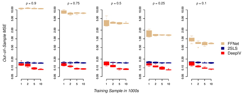
Our target counterfactual function is $\mathscr{h}(t,s,p)=s\psi_{t}+(\psi_{t}-2)p$. In out-of-sample evaluation, we compare estimated ${\hat{\mathscr{h}\mkern 4.0mu}\mkern-4.0mu}{}$ against the truth evaluated over a fixed grid of price values (with $[t,s]$ sampled as in the original DGP). This breaks the endogeneity that exists in the training sample, so that our out-of-sample errors are representative of the structural error that is of interest for counterfactual inference. In addition to Deep IV, we consider a regular feed-forward network (FFNet) and standard two-stage least squares (2SLS). We evaluate structural mean square error (MSE) while varying both the number of training examples and the amount of endogeneity. The results are summarized in Figure 2. Both 2SLS and our Deep IV model are designed to solve the endogeneity problem, and we see that their performance is mostly unaffected by changes in the amount of endogeneity. 2SLS is constrained by its homogeneity and linearity assumptions, so that it does not improve with increasing data. However, it still does much better than FFNet. This naive ML is doing a good job of estimating $\mathscr{h}(t,s,p)+\mathds{E}[e|p]$, but a terrible job of recovering the true counterfactual. As endogeneity drops, so that $\mathds{E}[e|p]$ decreases, FFNet improves. However even at low levels of endogeneity it remains far worse than simple 2SLS. In contrast, Deep IV is the best performing model throughout and its performance improves as the amount of data grows.

Figure 3: Bayesian (left) and Frequentist (right) inference for a central slice of the counterfactual function, taken at the average price and in our $4^{th}$ customer category. Since the price effect for a given customer at a specific time is constant in (27), the curves here are a rescaling of the customer price sensitivity function.

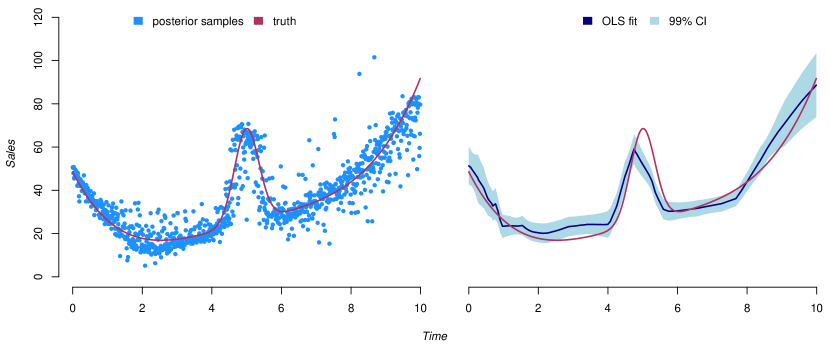
Figure 3 uses the Bayesian and Frequentist techniques from Section 4 to obtain uncertainty estimates for our model’s predicted sales over time. This is a slice of $\mathscr{h}$ evaluated at averages $p=25$ and $s=4$, trained on a large set of 1 million observations. Since expected sales for a given customer at a specific time are linear in price, the curves here are a rescaling of the customer price sensitivity function. This is the object that we need to recover for structural counterfactual inference. The Bayesian inference here is for an inverse dropout rate of $c=0.99$, which was tuned to be optimal in out-of-sample prediction. We see that DeepIV is able to mostly recover the true counterfactual shape. The Bayesian procedure provides wider uncertainty than the conditional inference obtained through data splitting, but this is completely determined by our choice of $c$. We have no strong argument for one inference procedure over the other at this time.

6 Discussion

The next generation of problems in ML involve moving from raw prediction tasks into more complex decision-making domains. In addition, we want our AI solutions to be transparent and to have the ability to respect notions of, e.g., fairness. All of these needs require a knowledge of the true structure of the processes that we are modeling and, hence, causal inference. The work in this paper is a step in the direction of Causal AI. The Deep IV framework shows that it is possible to take generic ML procedures, trained via SGD, and to use econometric theory to stack them together into a system that provides reliable answers to causal questions. This is a recipe for Artificial Economic Intelligence, and we think that much more can come from such an approach.

References

- Angrist et al. [1996] J. D. Angrist, G.W. Imbens, and D. B. Rubin. Identification of causal effects using instrumental variables. Journal of the American Statistical Association, 91(434):444–455, 1996.
- Angrist and Pischke [2008] Joshua D Angrist and Jörn-Steffen Pischke. Mostly harmless econometrics: An empiricist’s companion. Princeton university press, 2008.
- Athey and Imbens [2016] Susan Athey and Guido Imbens. Recursive partitioning for heterogeneous causal effects. Proceedings of the National Academy of Sciences, 113:7353–7360, 2016.
- Belloni et al. [2012] Alexandre Belloni, Daniel Chen, Victor Chernozhukov, and Christian Hansen. Sparse models and methods for optimal instruments with an application to eminent domain. Econometrica, 80:2369–2430, 2012.
- Belloni et al. [2014] Alexandre Belloni, Victor Chernozhukov, and Christian Hansen. Inference on treatment effects after selection among high-dimensional controls. The Review of Economic Studies, 81:608–650, 2014.
- Bishop [2006] Christopher M. Bishop. Pattern Recognition and Machine Learning. Springer, 2006.
- Blundell et al. [2007] Richard Blundell, Xiaohong Chen, and Dennis Kristensen. Semi-nonparametric iv estimation of shape-invariant engel curves. Econometrica, 75:1630–1669, 2007.
- Bottou [2010] L. Bottou. Large-scale machine learning with stochastic gradient descent. In Proceedings of COMPSTAT’2010, pages 177–186. Springer, 2010.
- Bound et al. [1995] John Bound, David A Jaeger, and Regina M Baker. Problems with instrumental variables estimation when the correlation between the instruments and the endogenous explanatory variable is weak. Journal of the American Statistical Association, 90:443–450, 1995.
- Bousquet and Bottou [2008] Olivier Bousquet and Léon Bottou. The tradeoffs of large scale learning. In Advances in neural information processing systems (NIPS), pages 161–168, 2008.
- Chamberlain [1987] Gary Chamberlain. Asymptotic efficiency in estimation with conditional moment restrictions. Journal of Econometrics, 34:305–334, 1987.
- Chen and Pouzo [2012] X. Chen and D. Pouzo. Estimation of nonparametric conditional moment models with possibly nonsmooth generalized residuals. Econometrica, 80:277–321, 2012.
- Chernozhukov et al. [2016] Victor Chernozhukov, Denis Chetverikov, Mert Demirer, Esther Duflo, Christian Hansen, and Whitney Newey. Double machine learning for treatment and causal parameters. arXiv preprint arXiv:1608.00060, 2016.
- Cox [1975] DR Cox. A note on data-splitting for the evaluation of significance levels. Biometrika, 62(2):441–444, 1975.
- Darolles et al. [2011] Serge Darolles, Yanqin Fan, Jean-Pierre Florens, and Eric Renault. Nonparametric instrumental regression. Econometrica, 79:1541–1565, 2011.
- Duchi et al. [2011] John Duchi, Elad Hazan, and Yoram Singer. Adaptive subgradient methods for online learning and stochastic optimization. Journal of Machine Learning Research, 12:2121–2159, 2011.
- Fithian et al. [2015] William Fithian, Dennis Sun, and Jonathan Taylor. Optimal inference after model selection. arXiv, 2015.
- Gal [2016] Yarin Gal. Uncertainty in Deep Learning. PhD thesis, University of Cambridge, 2016.
- Gal and Ghahramani [2015] Yarin Gal and Zoubin Ghahramani. Dropout as a bayesian approximation: Representing model uncertainty in deep learning. arXiv preprint arXiv:1506.02142, 2015.
- Hall and Horowitz [2005] Peter Hall and Joel L. Horowitz. Nonparametric methods for inference in the presence of instrumental variables. Ann. Statist., 33(6):2904–2929, 12 2005. doi: 10.1214/009053605000000714.
- Hornik [1991] Kurt Hornik. Approximation capabilities of multilayer feedforward networks. Neural networks, 4:251–257, 1991.
- Kingma and Welling [2013] D. P. Kingma and M. Welling. Auto-encoding variational Bayes. arXiv preprint 1312.6114, 2013.
- Kingma and Ba [2014] Diederik Kingma and Jimmy Ba. ADAM: A method for stochastic optimization. International Conference on Learning Representations (ICLR), 2014.
- LeCun et al. [2015] Y. LeCun, Y. Bengio, and G. Hinton. Deep learning. Nature, 2015.
- McFadden [1989] Daniel McFadden. A method of simulated moments for estimation of discrete response models without numerical integration. Econometrica, 57:995–1026, 1989.
- Newey and Powell [2003] W. K. Newey and J. L. Powell. Instrumental variable estimation of nonparametric models. Econometrica, 71(5):1565–1578, 2003.
- Pakes and Pollard [1989] A. Pakes and D. Pollard. Simulation and the asymptotics of optimization estimators. Econometrica, 57(5):1027–1057, 1989.
- Pearl [1995] Judea Pearl. On the testability of causal models with latent and instrumental variables. In Proceedings of the Eleventh conference on Uncertainty in Artificial Intelligence (UAI), pages 435–443, 1995.
- Reiersøl. [1945] O. Reiersøl. Confluence analysis by means of instrumental sets of variables. Arkiv för Matematik, Astronomi och Fysik, 32a(4):1–119, 1945.
- Robbins and Monro [1951] H. Robbins and S. Monro. A stochastic approximation method. The Annals of Mathematical Statistics, pages 400–407, 1951.
- Rosenbaum and Rubin [1983] P. R. Rosenbaum and D. B. Rubin. Assessing sensitivity to an unobserved binary covariate in an observational study with binary outcome. Journal of the Royal Statistical Society. Series B (Methodological), 45(2):212–218, 1983.
- Schmidhuber [2015] J. Schmidhuber. Deep learning in neural networks: An overview. Neural Networks, 2015.
- Srivastava et al. [2014] Nitish Srivastava, Geoffrey E Hinton, Alex Krizhevsky, Ilya Sutskever, and Ruslan Salakhutdinov. Dropout: a simple way to prevent neural networks from overfitting. Journal of Machine Learning Research, 15:1929–1958, 2014.
- Taddy et al. [2016] Matt Taddy, Matt Gardner, Liyun Chen, and David Draper. Nonparametric Bayesian analysis of heterogeneous treatment effects in digital experimentation. Journal of Business and Economic Statistics, 2016. to appear.
- Wager and Athey [2015] Stefan Wager and Susan Athey. Inference of heterogeneous treatment effects using random forests. arXiv:1510.04342, 2015.
- White [1980] Halbert White. A heteroskedasticity-consistent covariance matrix estimator and a direct test for heteroskedasticity. Econometrica, 48, 1980.
- Wright [1928] P. G. Wright. The Tariff on Animal and Vegetable Oils. Macmillan, 1928.
- Zinkevich [2003] Martin Zinkevich. Online convex programming and generalized infinitesimal gradient ascent. In Proceedings of the Twentieth International Conference on Machine Learning (ICML), 2003.