Reference Manual
PrASP111Version 0.9.4 Report
Matthias Nickles
College of Engineering & Informatics
National University of Ireland, Galway
University Road 1, Galway City, Ireland
matthias.nickles@deri.org
Abstract. This technical report describes the usage, syntax, semantics and core algorithms of the probabilistic inductive logic programming framework PrASP. PrASP is a research software which integrates non-monotonic reasoning based on Answer Set Programming (ASP), probabilistic inference and parameter learning. In contrast to traditional approaches to Probabilistic (Inductive) Logic Programming, our framework imposes only little restrictions on probabilistic logic programs. In particular, PrASP allows for ASP as well as First-Order Logic syntax, and for the annotation of formulas with point probabilities as well as interval probabilities. A range of widely configurable inference algorithms can be combined in a pipeline-like fashion, in order to cover a variety of use cases.
Keywords: Artificial Intelligence, Uncertainty Reasoning, Logic Programming, Answer Set Programming, Probabilistic Inductive Logic Programming, Probabilistic Programming
1 Introduction
PrASP [28, 30, 32, 31, 29] (Probabilistic Answer Set Programming) is a Nilsson-style [11] probabilistic inductive logic programming (PILP) language (e.g., [5, 6, 13, 16, 18, 20, 12, 23, 10, 22, 42, 43]) and an uncertainty reasoning and statistical relational machine learning software, based on Answer Set Programming (ASP) [1, 2]. PILP is a form of declarative logical/relational probabilistic programming and ASP is a form of non-monotonic logic programming whose syntax is similar to that of Prolog but whose inference approach is more closely related to SAT, constraint satisfaction problem solving and Satisfiability Modulo Theories (SMT) solving. Besides probabilistic ASP, PrASP also includes limited support for inference with probabilistic normal logic programs under non-ASP-based semantics (mainly for research and benchmarking purposes).
1.1 Properties
- High degree of expressiveness
-
PrASP provides a unified framework with support for Answer Set Programming (ASP) and First-Order Logic (FOL) syntax, interval probabilities (as in probability bounds analysis), conditional probabilities and Annotated Disjunctions [27]. Arbitrary logic formulas can be directly annotated with probabilities or probability intervals.
- Flexible inference approaches
- Non-monotonic logic programming
-
Being based on Answer Set Programming, PrASP can be used for probabilistic non-monotonic reasoning. As a logic programming approach, it is able to handle inductive definitions (in contrast to approaches like MLN [18] which are based on FOL or fragments thereof, such as Description Logic).
- No mandatory independence assumption.
-
In contrast to many other PILP frameworks and probabilistic databases, PrASP does, by default, not assume probabilistic independence of uncertain events. However, some of its inference algorithms can make use of event (formula) independence in order to speed up inference.
- Uncertainty reasoning with annotated as well as unannoted formulas
-
PrASP approach to nondeterminism is essentially based on logical disjunction. Therefore, it provides seamless interoperability of probabilistically annotated statements and plain disjunctions or ASP choice constructs for the modeling of nondeterminism.
- Parameter learning.
-
PrASP can be used to learn the probabilities of given hypotheses from example data. This is a form of Inductive Logic Programming (ILP) which in the area of ASP has so far mainly been approached in the form of non-probabilistic induction of new hypotheses (structure learning) [25].
- Markov Logic
-
semantics is (experimentally) supported using switch
--mlns, in the sense of [20], i.e. combined with stable model semantics. In contrast to the original Markov Logic Networks, [20] and PrASP (with its own semantics as well as--mlns), being based on logic programming rather than classic FOL, support inductive definitions. (Note that with its native semantics, PrASP is not much related to MLN, apart from the fact that both frameworks support FOL syntax.) - Platform independence.
-
PrASP is programmed in Scala and thus runs on the widely available Java Virtual Machine (JVM)222Optionally, it can make use of native code libraries to improve performance on certain platforms.. Its API can be used with Java, Scala, Clojure, Groovy and other languages which run on the JVM, and with other JVM-based frameworks (such as Spark). However, for certain procedures (such as Linear Least Squares), PrASP uses platform-dependent external libraries where available (such as CUDA), and Java code as a fallback.
- Extensible syntax
-
using macros written in the Scala programming language
- Streaming data
-
in RDF format can be used as input for inference and learning tasks (experimental feature).
However, it should also be noted that the current version of PrASP is a research prototype which might still have a few rough edges. If you encounter bugs or if you want to suggest improvements of the framework or its documentation, please don’t hesitate to contact the developer (see Sect. 9).
Background knowledge (PrASP programs) can be uncertain (by attaching probabilities or probability intervals to formulas). Besides the native Prolog-like input language AnsProlog, it is also possible to use formats such as First-Order Logic (FOL, using translation provided internally by PrASP itself or using an external translator such as F2LP [3]), action languages [33] and planning languages such as PDDL [36] as input languages (with the help of external conversion tools). In addition to these syntax forms, so-called Annotated Disjunctions are supported as “syntactic sugar” (in a similar way as in ProbLog).
At this, PrASP imposes virtually no restrictions on the annotations of formulas with probabilities, although of course not all syntactically valid PrASP programs are consistent or efficient.
PrASP includes a number of inference approaches, including linear equation system solving, simulated annealing, iterative refinement (using the approach from SPIRIT [16]), model counting, and linear programming (LP). Inference algorithms are described in Section 5. Currently supported inference tasks are computation of the conditional and non-conditional probabilities of given formulas (query formulas), computation of probability bounds of query formulas, and MAP (Maximum A-Posteriori) inference (computing the most probable world). Parameter learning allows to compute the probabilities of given hypotheses inductively from learning examples and background knowledge.
1.2 Overview
Background knowledge (uncertain as well as certain knowledge provided by some domain expert) is given in form of a PrASP program (a probabilistic logic program). It provides a set of constraints for the set of possible worlds as well as for the valid probability distributions over those possible worlds. In PrASP terminology, possible worlds are also called models and correspond to the answer sets333The idea to associate possible worlds with answer sets stems from [10]. of the so-called spanning program [30] of the PrASP program 5. For probabilistic inference, PrASP computes one such probability distribution from the given background knowledge and subsequently uses this probability distribution to compute precise or approximate unconditional or conditional probabilities of the query formulas (formulas whose probabilities the user wants PrASP to compute). Given the constraints specified by the PrASP program, each query might have multiple solutions (or more precisely, a range of probabilities), of which PrASP by default computes only a single point probability per query formula444Unless command-line arguments --intervalresults or --ndistrs n with are specified, see Section 6.3.
A PrASP program can contain formulas in ASP syntax (AnsProlog) as well as formulas in first-order logic (FOL) syntax, which allows for a wide range of applications (e.g, using Event Calculus axioms for probabilistic reasoning about actions and other events). Other formats require conversion to ASP before PrASP is called, using some appropriate translation software. ASP and FOL formulas can coexist within the same PrASP program, however, you should not mix both styles within the same formula.
Any formula can be annotated (parameterized) with a probability or an interval of probabilities, in order to specify uncertain beliefs. Such an annotation is called the weight of the respective formula.
It is furthermore possible to specify conditional probabilities explicitly in background knowledge, although in many case Annotated Disjunctions should be considered as a computationally cheaper alternative.
Formulas can contain variables (ASP-style as well as FOL variables), however, “first-order” inference is restricted to finite discrete domains.
Given the background knowledge, PrASP can infer conditional as well as unconditional probabilities of ground and non-ground query formulas. Weights of given hypotheses can also be learned inductively from example data. Such examples can in principle be arbitrary formulas, but typically they are ground atoms.
Background knowledge in form of a PrASP program is provided by the user as a file with file name ending .prasp. Such a file consists of a set of weighted or unweighted logical formulas, plus optionally meta-statements. Each formula must be concluded by a dot (”.”) and must not contain line breaks555For the sake of better readability, we often omit the concluding dot in this document..
Besides PrASP programs, there are also query files (which consist a number of query formulas whose weights should be computed by inference), files with hypotheses (formulas whose weight should be learned from examples) and learning examples. Examples for these tasks are provided later in this document, in a tutorial-style section (Sect. 3).
Here’s an example for background knowledge (i.e., a PrASP program) in native annotated AnsProlog syntax. Note that constants and predicates need to start with a lowercase letter whereas variables start with an uppercase letter.
[0.45;0.5] coin(1,heads).
[[0.5]] coin(X,heads) :- X != 1.
win :- coin(1,heads), coin(2,heads).
Formulas such as [0.5] coin(2,heads) are annotated with probabilities (weights). Weights can be attached to any kinds of formulas (ground or non-ground facts and rules). In contrast to the types of weights found in some other probabilistic languages, the numbers within the square brackets are actual probabilities (e.g., ) or probability intervals.
Weights come in various syntactic forms, the most simple one being the form [], where is a probability. Probability intervals [;] can also be used as weights. The informal meaning of a formula annotated with weight [] is that this formula has the probability (that is, represents a random event and ). Weights can be attached to all kinds of formulas in the background knowledge, including rules, facts, disjunctions, and formulas with existential or universally quantified variables over finite domains. For example,
[0.7] p(X) :- q(X). specifies that the probability of non-ground rule p(X) :- q(X) is . Formulas which contain variables (here X) are called non-ground. Weighted non-ground formulas are interpreted as weighted conjunctions of ground formulas, if a single-square bracket annotation is used (there are other forms of annotations too, with different semantics, as explained later).
However, of course not all syntactically valid PrASP programs are equally suitable for time- and memory efficient inference and learning. Therefore a significant part of this document is concerned with inference and optimization methods supported by PrASP , each with different characteristics in terms of speed, accuracy, requirements etc, in order to facilitate a wide range of different use cases for inference and learning (learning makes internally heavy use of inference).
Note that PrASP does not necessarily assume probabilistic independence of formulas for which
no logical dependence (e.g., by means of some logical rule which relates two random events) is specified. Again in contrast to many other probabilistic logics, the user can specify which sets of formulas should be treated as independent and which kind of independence should be assumed. E.g., in the program above, coin(1,heads) and coin(2,heads) could be explicitly declared as pairwise independent (by adding a certain meta-statement 4.7 or indirectly using conditional probabilities), or their independence could be left unspecified (e.g., in order to compute interval results of all possible query outcomes), or automatically discovered by PrASP . Independence assumptions
can have a tremendous influence on inference performance, as they allow for certain simplifications which
are not possible otherwise. On the other hand, inference algorithms which cannot apply such simplifications are slowed down (!) if event independence is being assumed.
Various other types of weights exist. E.g., Computed weights allow for symbolic weights whose numerical values are computed during grounding666“Grounding” means that an ASP program with variables is replaced by an equivalent program without variables. Most ASP solvers require grounded input. Grounding is either performed by a separate grounding tool or by a combined grounder/solver. Contemporary ASP grounders typically also perform simplifications during grounding by removing ground formulas of which they know cannot be true. Grounding can be limited by using simplification switches such as --mod1. (either using ASP or using a procedural scripting language) or random weights. For details, please see Section 4.4.
It is possible to specify conditional probabilities directly in background knowledge, using the following weight annotation syntax: [|] . This declares that , i.e., that the probability of is w, given that we already know that holds. Both and are formulas. While within formulas, symbol | stands for logical disjunction, here its first occurrence in annotation [|] separates the probability from probabilistic condition .
Example: [0.75|not sunny] rainy | snowy specifies that the probability that it is either rainy or snowy is 0.75, given that we know it’s not sunny. Conditional probabilities in background knowledge come with a performance penalty though, and alternatives available in PrASP , such as certain patterns of annotated rules (Sect. 3) or Annotated Disjunctions (Sect. 3.2), should be considered.
Like in any formulas, variables, logical connectives, etc., logical variables are allowed both within f and the condition formula c.
It is possible to specify weights in conditional as well as unconditional probabilities using so-called double- or triple-square notion (e.g., [[|]] or [[[]]]), in order to declare uncertain ground instances of non-ground formulas in compact form (see Sect. 4.4). Variables can be used within ordinary weighted formulas (single-square annotations) too, but the semantics is different from double- or triple-square notion (see Sect. 4.4).
PrASP can discover and warn against probabilistically inconsistent weight annotations (e.g., if the background knowledge contains both [0.3] p and [0.9] not p), provided the default inference approach is being used (so-called “PrASP vanilla” mode), but basically it is the responsibility of the user to provide probabilistically and logically consistent background knowledge.
Formulas in ASP syntax can contain most of the syntactic constructs supported by contemporary ASP grounders, such as aggregates. FOL syntax is by default as specified for the input language of F2LP [3] (which is akin to the TPTP format), although it is also possible to use the PrASP -internal FOLASP converter (which uses almost the same formula syntax, see switch --folconv for details) or other external converters.
In accordance with AnsProlog customs, variable names need to start with an upper-case letter and constants need to start with a lower-case letter. The domains of quantified variables in formulas using FOL-syntax need to be finite (because FOL-formulas are translated into ASP programs).
PrASP programs can contain meta-statements understood by the respective external ASP grounding tool, such as as domain declarations, as well as various PrASP -specific meta-statements (see Section 4.7). Meta-statements start with character #.
Like plain ASP, PrASP distinguishes between classical negation and default negation. Prefix “-” denotes strong (classical) negation and prefix “not” stands for default negation, as usual. Note that PrASP works by default with default negation in order to implement (as an experimental feature which might disappear in future versions, this behaviour can be switched to the use of classical negation).
Important: PrASP ’s default settings are rather conservative - by specifying an algorithm and parameters which are specific to the respective inference problem, inference (and indirectly learning) speed can be massively increased (see Section 3.13 for simple approaches to achieve this).
The remainder of this technical report is organized as follows:
-
•
Section 2 describes how to install PrASP.
-
•
Section 3 provides an informal introduction to the use of PrASP for basic inference and learning tasks, as well as tips for performance tuning.
-
•
Section 4 describes PrASP’s syntax.
-
•
Section 5 describes its semantics, and core inference and learning algorithms.
-
•
Section 6 describes the software’s command line options.
-
•
Section 7 provides miscellaneous hints for troubleshooting.
-
•
Section 8 contains answers to frequently asked questions.
-
•
Section 9 contains developer contact details and a disclaimer.
2 Installation & Web Interface
Installation of PrASP is easy, since on most machines it only requires unzipping a file archive and copying one or two additional tools into the resulting directory. There needs to be a recent version of Java (Java 8 or newer, 64bit version). If you just want to quickly try out PrASP online, there’s also the PrASP Web Interface.
2.1 Web Interface
The PrASP Web Interface for online inference and learning can be found at
http://ubuntu1.it.nuigalway.ie:8977/PrASP_WebInterface/static/ABOUT.html
However, it is limited in several respects compared to the installable version of PrASP and
only suitable for small tasks.
2.2 Installation steps
-
1.
Unzip
prasp.zipinto a new directory (henceforth called the PrASP directory). Make sure PrASP has writing access to this directory. There is no installation program. -
2.
Put third-party external tools directly into the PrASP directory, if they are not already there. See below for the list of these tools (of which some are required and others are optional but strongly recommended). Make sure the filenames of their executables are as specified below (so that PrASP finds them). However, some of these tools might be already installed and ready to be used, depending on the PrASP file archive you have. See Sect. 2.3 for details.
-
3.
PrASP can optionally call native code for faster inference on the CPU or a Nvidia GPU. By default, PrASP expects native BLAS/LAPACK libraries. Under Windows and Mac OS X, normally no additional installation is required in this regard, unless you want to install your own BLAS implementation. Under Linux,
sudo apt-get install libatlas3-base libopenblas-baseis normally sufficient (tested with Debian/Ubuntu).
You can also disable the use of native BLAS/LAPACK altogether, see Sect. 2.5.
As for native GPU code, installation of additional libraries is normally not required, but see Sect. 2.5 for exceptions (in particular for Mac OS X). See --linsolveconf for how to activate native solver code. -
4.
If you are using Mac OS X or Linux, you should make
prasp.shexecutable usingchmod +x prasp.sh -
5.
Enter
./prasp.sh examples/example1.prasp examples/example1.query(Linux, MacOSX) orprasp.bat examples/example1.prasp examples/example1.query(Windows) for a first test of your installation777Example 1 is in Gringo 4 syntax. If you are using a different ASP grounder, you might need to tweak it a bit.. -
6.
It is highly recommended to read the rest of this section too (even if you already successfully ran the example), in particular Subsection 2.3.
2.3 External tools
As a minimum, you should888It is possible to perform a - very limited - range of probabilistic inference tasks without any ASP grounder or solver, e.g., MAP inference using --maxwalksat. Also, PrASP contains its own grounder which is able to ground basic non-ground formulas during the preprocessing phase. have an ASP grounder (recommended: Gringo [36]) and an ASP combined grounder/solver (recommended: Clingo [36]) installed.
The other external tools listed below (F2LP [3], CVC4 [4]) are recommended in order to make full use the framework but not strictly required.
All of the tools listed below are open source and available in binary form for Linux, MacOSX and Windows. Depending on your PrASP distribution, some of them might already be installed.
To install, simply copy these tools into the top PrASP directory if they aren’t already there, and make sure that the names of their executable binary files are exactly as specified below (so that PrASP can find them).
- - Clingo and Gringo
-
[36] are the most appropriate ASP grounder and solver for PrASP. They can be obtained from
http://potassco.sourceforge.net/. You need to decide if you want to use version 3 or version 4 (or higher) of these tools. Each of these versions has its pros and cons wrt. PrASP, see Sect. 2.4. If you are unsure which version to use, choose Clingo 4 and Gringo 4.Installation: Copy both tools into the top PrASP directory and make sure that the names of the executable files are gringo and clingo under Linux, clingo_macosx and gringo_macosx under Mac OS X, and clingo.exe and gringo.exe if you are using Windows.
If these files are already in your PrASP folder and you are fine with their versions (check with --version), you don’t need to do anything. You can switch between Clingo3/4 and Gringo3/4 using shell scripts
toggle...Other ASP grounders/solvers might also work if they are compatible with Lparse/Smodels or the ASP language standard. For DLV code whose syntax goes beyond the common ground with Lparse/Gringo, a converter such as
dlvtogringo999http://potassco.sourceforge.net/labs.html might be helpful (but we haven’t tested this yet). See --grounder and --groundersolver for how to specify different ASP grounder/solvers. - - F2LP
-
[3] (optional) is an external tool for translating program in FOL syntax (under the stable model semantics) into ASP logic programs. It can be obtained from
http://reasoning.eas.asu.edu/f2lp/. You can alternatively use PrASP’s built-in FOLASP converter FOL2ASP, which is active by default (or tell PrASP not to use any converter at all, which increases performance but obviously restricts you to ASP syntax). FOL2ASP provides better support for Gringo/Clingo 4 (as of May 2016), however, F2LP is still somewhat more mature.
Our recommendation is to try with the internal converter first if you are using Gringo/Clingo 4 or higher, and to install F2LP if you are still using Gringo/Clingo 3 or if you experience difficulties with the current (beta) version of the internal converter. You can switch between both at any time using --folconv.Installation: Copy the tool into the top PrASP directory. The name of the executable binary file must be f2lp§ (Linux), f2lp.exe (Windows) or f2lp_macosx (Mac OS X) in order to be discovered by PrASP .
- - CVC4
-
[4] (optional, strongly recommended) can be obtained from
http://cvc4.cs.nyu.edu. CVC4 is a SMT solver which is invoked by PrASP if the built-in linear system solver couldn’t find a solution or if there are intervals in weight annotations and the “vanilla” approach to inference is used (however, it is recommended to specify switch--intervalresultsin that case, which activates a different solver which deals with intervals much faster than CVC4). CVC4 is not strictly required, but its installation is strongly recommended.Installation: Simply copy the tool (including its external libraries) into the top PrASP directory. Its executable name must be cvc4 (Linux), cvc4_macosx (Mac OS X) or cvc4.exe (Windows). On a Mac, you might need to create the CVC4 executable first from
cvc4-1.2_3.mpkg(or newer), see below for details. To check if CVC4 is already installed, call PrASP with option --enforceSMT.
Further installation hints
-
•
On a Mac, the installation of CVC4 might require one further step: First, check if CVC4 is already installed by calling PrASP with option --enforceSMT. If you receive an error message indicating that no SMT solver was found, please install CVC4 using
cvc4-1.2_3.mpkg, copy the resulting executable file from/opt/local/bininto the PrASP folder and rename this file tocvc4_macosx -
•
Other ASP grounders/solvers than Gringo/Clingo might be usable as well, to varying degrees, if they are compatible with Lparse/Smodels or the ASPCore-2 language standard. To specify a different grounder/solver use command-line arguments --grounder and --groundersolver.
PrASP also supports the combined ASP / Constraint Satisfaction Problem (CSP) solver clingcon [36]. To use clingcon, specify--groundersolver clingconon the command-line. -
•
If you can obtain or build the (non-default) portfolio binary
pcvc4of CVC4 with multi-threading enabled, this is preferred over the default version of CVC4. If you are using the portfolio binary, invoke PrASP with command-line option--SMTsolver pcvc4(ifpcvc4is the name of the executable binary). For Linux 64bit, pre-build portfolio binaries might be available fromhttp://cvc4.cs.nyu.edu/cvc4-builds/portfolio-x86_64-linux-opt/ -
•
Note that PrASP works generally faster if only ASP syntax is used and command-line option
--folconv none is specified. -
•
Modify the PrASP start script
prasp.sh(Linux, Mac OS X) orprasp.bat(Windows) if necessary. In particular, make sure that ajavais found and that the amount of heap memory assigned to Java is large enough (in case you encounter “out of memory” errors). -
•
The current version of PrASP requires at least a Java JRE 8. If you cannot install Java 8 (=1.8) or higher on your system (or in case of any other installation problem), please contact the PrASP developer for advice (see Sect. 9).
2.4 About Gringo / Clingo 4 vs. 3
The ASP examples in this document are mostly still in Gringo/Clingo 3 syntax, however, since v0.8.10, PrASP also supports most of Gringo/Clingo 4 syntax (and the amount of supported syntax will be further increase in future PrASP versions). Gringo/Clingo 4 are already preferred over version 3 for most PrASP use cases.
Gringo/Clingo 4 provides significant advantages over older versions in connection with PrASP, in particular wrt. sampling performance. There are a few issues too though… In detail, Clingo/Gringo 4
…allow for (fast) remote sampling (which is active by default if PrASP discovers Clingo 4 - see switch --noremotesampling for details).
…aren’t fully compatible with the external FOLASP converter F2LP (at least up to version 1.3). If you experience issues, you might want to specify the internal converter (which is automatically used if you don’t install F2LP) or deactivate FOL conversion altogether using command-line argument --folconv.
…support and require ASP standard syntax
(https://www.mat.unical.it/aspcomp2013/ASPStandardization). Beware that some of the differences compared to Gringo 3/Lparse syntax are quite subtle wrt. their effect (e.g., for aggregates), see Gringo/Clingo 4 user manual.
…do not yet allow for automated discovery of formula independence.
Please refer to the Gringo/Clingo 4 manual for any required syntax modifications if you want to use Gringo/Clingo 4. Note that many of the syntax differences are very simple where a few others are quite subtle, in particular for non-trivial aggregate constructs such as #count.
Scripts toggleClingo3to4.sh and toggleClingo4to3.sh (Mac OS X, Linux) and
toggleClingo3to4.bat and toggleClingo4to3.bat (Windows) switch between Gringo/Clingo 3 and 4, simply by renaming/copying the respective Gringo/Clingo executables files so that PrASP uses them by default. Alternatively, the grounder and grounder/solver can be specified using command-line options --grounder and --groundersolver.
2.5 Native libraries
PrASP can optionally make use of native CPU and/or GPU code in order to speed up inference.
If you want to make use of this, there are the following groups of libraries to consider during installation. After installation, call PrASP with option --linsolveconf to configure the use of native solver code. Note that currently only the “vanilla” approach to inference makes use of native code, so even with this, speed is rather low compared to approximate inference approaches.
- BLAS/LAPACK libraries (CPU):
-
Mac OS X and Windows users normally don’t need to install additional libraries in this regard, as these libraries are either already included with the operating system (CPU LAPACK/BLAS code on MacOSX) or with PrASP itself. However, with regard to LAPACK/BLAS under Linux and Windows, it might make sense to install variants of these which provide higher performance compared to the default ones.
To install native BLAS/LAPACK libraries under Linux (tested with Debian/Ubuntu), do, e.g., the following in order to install OpenBLAS (but there are alternative BLAS/LAPACK implementations too):
Ψsudo apt-get install libatlas3-base libopenblas-base
Ψsudo update-alternatives --config libblas.so
Ψsudo update-alternatives --config libblas.so.3
Ψsudo update-alternatives --config liblapack.so
Ψsudo update-alternatives --config liblapack.so.3
See
https://github.com/fommil/netlib-java/for details. You might need to editprasp.shorprasp.batafterwards.
You can configure which BLAS/LAPACK installation is used using the-Dcom.github.fommil.netlib… arguments inprasp.shorprasp.bat(Windows).
Again, seehttps://github.com/fommil/netlib-java/for details.To deactivate the use of native BLAS/LAPACK libraries, change the
-Dcom.github.fommil.netlib.BLAS,-Dcom.github.fommil.netlib.LAPACK,-Dcom.github.fommil.netlib.ARPACKparameter values in thejavacall inprasp.shorprasp.batto-Dcom.github.fommil.netlib.BLAS=com.github.fommil.netlib.F2jBLAS -Dcom.github.fommil.netlib.LAPACK=com.github.fommil.netlib.F2jLAPACK -Dcom.github.fommil.netlib.ARPACK=com.github.fommil.netlib.F2jARPACK
- Native CUDA libraries (Nvidia GPUs):
-
Under Linux and Windows, this should work without the need to install additional libraries, since the necessary redistributable runtime CUDA libraries are part of PrASP . However, you might have to update your Nvidia graphics card driver to enable CUDA 7. Installing the (free) CUDA 7 Toolkit (
https://developer.nvidia.com/cuda-toolkit-archive) is one possibility to ensure that your system have the correct driver installed. Also, relevant runtime libraries, if still needed, can be obtained this way (but you won’t need the compiler and other developer tools included in the toolkit).Under Mac OS X, it is recommended to install the free CUDA 7.0 Toolkit
(https://developer.nvidia.com/cuda-toolkit-archive), this should automatically provide suitable native CUDA libraries. If you experience ”Image not found” errors on El Capitain (due to a well known issue with this platform), seeprasp.shfor a possible workaround.
3 Working with PrASP
3.1 Basic probabilistic inference
3.1.1 Invoking PrASP for query answering
For probabilistic inference, PrASP is typically called as follows:
./prasp.sh101010With Windows, use prasp.bat instead of prasp.sh. <file1.prasp> <file2.query>
<file1.prasp> is a PrASP program file which represents the available certain and/or uncertain background knowledge, that is, the probabilistic and non-probabilistic rules and facts from which the query answers can be inferred. The syntax of background knowledge is described in Sections 1.2 and 4.
<file2.query> is the query file, consisting of a number of query formulas of the form [?] f. or [?|c] f. or [[?]] f. or [[?|c]] f. or [[[?|c]]] f.
With these arguments, PrASP is instructed to compute the probabilities of the query formulas, i.e., to find concrete values for the question marks in the formula annotations.
The file name extensions need to be .prasp for the background knowledge file and .query for the query file.
The command line above is an abbreviation of -b <file1.prasp> -q <file2.query>.
Using the latter form, the file name extensions don’t need to be .prasp / .query.
For programs with a large number of answer sets and/or a large number of query formulas in the query file, it is recommended to provide additional command-line arguments in order to speed up inference. Please see Section 3.13 for details.
Results are written to stdout.
A query file (<file2.query> above) can contain multiple query formulas.
There are several syntax forms for query formulas: use [?] to obtain an approximation of the unconditional probability of . Use [?|] to get an approximation of the conditional probability of given . Both and can be any formulas (in ASP or FOL syntax). is typically the observed evidence. Later in this document further forms of query formulas (using double- and triple-square bracketed weights) will be introduced.
Resulting probabilities are represented in the form [computedWeight] queryFormula. Conditional probabilities are displayed in the form [p|] .
In case PrASP couldn’t compute the probability of a query formula for some reason, [?] queryFormula is returned.
Conditional probabilities can also be used in background knowledge using syntax [p|] (like all formulas, they need to be concluded by a dot). See further below in this section for examples and computationally more efficient alternatives.
Numerical weights are not allowed within query files. But optionally, unannotated formulas and #domain meta-statements can be put in the query file in order to specify domain predicates for the bindings of variables, which is useful if the respective domains are only needed in query formulas (otherwise, domains and domain predicates can simply be specified in the background knowledge file, like any other facts).
In case of large programs, inference and learning becomes tractable only by activating program optimizations or approximation algorithms such as --itrefinement, simplification of conjunctions of independent formulas (command-line option --mod0), modularization (command-line option --mod1) or --simanneal. Shortcuts for combinations of certain optimization-related switches are -o1, -o2, -o3, etc. (see 6.3). However, optimization measures might lead to less accuracy. Details about how to improve inference or learning speed are described in Sect. 3.13 and in Sect. 6.3.
3.1.2 A first example: Coin flipping
Here’s a first simple example for probabilistic inference. Let’s assume we want to model a simple coin tossing game with two independent coins (coin1 and coin2). If both coins show “heads”, the player wins. The first coin is biased (heads appears with probability 0.6). We will later see how to model this scenario more elegantly using variables, but for the moment, we stick to a simple formalization and store the following PrASP program in file kb1.prasp (the background knowledge):
#indep
[0.6] coin1(heads).
[0.5] coin2(heads).
#endIndep
1{coin1(heads),coin1(tails)}1.
1{coin2(heads),coin2(tails)}1.
win :- coin1(heads), coin2(heads).
We are now interested in the probability of winning the game, and in various other probabilities inferable from the background knowledge. We put the following queries into file test1.query:
[?] coin1(tails).
[?] coin2(heads).
[?] coin1(heads) | coin1(tails).
[?] not (coin1(heads) | coin1(tails)).
[?] coin1(heads) & coin2(heads).
[?] win.
[?|coin1(heads) & coin2(heads)] win.
Calling PrASP using
./prasp.sh111111With Windows, invoke prasp.bat instead of prasp.sh. From now on, we omit denoting the start script. kb1.prasp test1.query
gives the following results:
% query1.query

[0.4] coin1(tails).
[0.5] coin2(heads).
[1] coin1(heads) | coin1(tails).
[0] not (coin1(heads) | coin1(tails)).
[0.3] coin1(heads) & coin2(heads).
[0.3] win.
[1|coin1(heads) & coin2(heads)] win.
The first line tells us that the probability that coin number 1 comes up with “tails” is 0.4. This follows from the
fact that the probability of “heads” is 0.6 for this coin and that formula 1{coin1(heads),coin1(tails)}1 in the background knowledge
enforces that in each possible world either coin1(heads) or coin1(tails) is true, but never both together.
[1] coin1(heads) | coin1(tails) means that the probability that either “heads” or “tails” appears is 1.0, and
[0.3] coin1(heads) & coin2(heads) denotes probability 0.3 for the event that both coins show “heads” after being tossed, which is also the unconditional probability of win, i.e., of winning the game. Observe that formula coin1(heads) & coin2(heads) is in FOL/F2LP [3] syntax.
The last result line ([1.00|coin1(heads) & coin2(heads)] win) reads:
“The probability of win given that we know that coin1(heads) & coin2(heads) holds is 1.00” (that is, ).
The example also show that ASP and FOL syntax can be freely mixed in PrASP programs and queries (albeit not within the same formula). However, the semantics for the non-probabilistic part of our logic is always the stable model semantics used in Answer Set Programming - first-order formulas are internally transformed into equivalent ASP constructs (more precisely, into disjunctive logic programs).
3.1.3 Probabilistic inference in the absence of weighted beliefs
Probabilistic inference does not necessarily rely on the presence of weighted formulas in the background knowledge. Consider the following variant of the famous “Tweety”-example for non-monotonic logic programming [37]:
fly(X) :- bird(X), not neg_fly(X).
neg_fly(X) :- bird(X), not fly(X).
neg_fly(X) :- penguin(X).

bird(tweety).
chicken(tweety).
bird(tux).
penguin(tux).
We store this as a .prasp file and put the following into the .query file:
[?] fly(tux).
[?] fly(tweety).
The inference result is
[0] fly(tux).
[0.5] fly(tweety).
We get these results because our background knowledge encodes that Tux is a penguin and penguins definitely don’t fly, whereas Tweety is not a penguin and thus Tweety may fly or not. Due to entropy maximization (which will be addressed later), the uncertainty about whether Tweety can fly or not is quantified as 0.5 (which is exactly “in the middle” between 0 (cannot fly) and 1 (can fly)).
If we call PrASP with switch --intervalresults, we obtain
[0;0] fly(tux).
[0;1] fly(tweety).
This also reflects our uncertainty about Tweety’s flying capability. However, in contrast to the previous result, it shows the full range of probabilities instead of a point probability.
3.1.4 Weighted rules and conditional probabilities
How about weighted rules? Let’s get back to the coin flipping example (3.1.2) and add the following to the background knowledge (i.e., file kb1.prasp):
[0.8] happy :- win.
With the following additional queries:
[?] happy.
[?|win] happy.
…we get, maybe surprisingly, the following results:
...
[0.1] happy.
[0.333333333|win] happy.
Why that? The reason is that [0.8] happy :- win does not denote the conditional probability 0.8 of being happy given win, but instead the probability 0.8 of the event which is specified as the logical implication , i.e. .
This exemplifies that in general, logical rules do not correspond to conditional probabilities. Examples for proper use of weighted rules are shown further below in this document. Anyways, in order to specify the conditional probability , we could replace
[0.8] happy :- win in the background knowledge with the following two lines:
[0.8|win] happy.
:- happy, not win.
(The last line expresses that there shall be no happiness without winning.) Now the query results are as expected:
...
[0.24] happy.
[0.8|win] happy.
Note that conditions (the formulas between ”|” and ”]”) are not restricted to facts, they can be any formulas.
Remark: the probabilities of all conditioned as well as unconditioned weighted formulas (both in the background knowledge and in queries) are implicitly conditioned on the background knowledge, or more precisely, on the so-called spanning program - what that exactly means will be described later, but basically it just says that each weighted formula has the conjunction of all non-weighted formulas in the background knowledge as its implicit condition (or as its implicit additional condition, in case the weight of the formula is already in conditional form [p|c]).
Despite their convenience, specifiation of conditional probabilities in background knowledge are computationally quite expensive. A computationally cheaper approach supported by PrASP (and certain other PLP frameworks, such as ProbLog) is to use so-called Annotated Disjunctions [27], see Sect. 3.2 for details. But for now, we just emulate the effect of Annotated Disjunctions manually, by replacing
[0.8|win] happy.
:- happy, not win.
with
[0.8] h.
happy :- win, h.
The last two lines correspond to annotated disjunction 0.8::happy :- win in ProbLog syntax - the annotation 0.8:: refers to the head of the rule (happy), not to the entire rule as in PrASP . We will later introduce a more convenient syntax for annotated disjunction.
Note that their semantics is not the same as that of the statements above with the conditional probability.
Observe that PrASP does by default not assume any specific prior probability distribution over uncertain atoms or clauses whose probabilities are not specified by the user (or deducible using rules, etc).
For formulas which appear nowhere in a rule head, inference computes, in accordance with stable world semantics, probability 0, i.e., it makes a closed-world assumption which is typical for logic programming.
Consider the following example background knowledge file, which consist only of a single line:
[0.6|friend(brad, janet)] influences(brad, janet).
If we issue query [[?|friend(brad, janet)]] influences(brad, janet) to test whether the inference result reflects the given background knowledge, the result is
[?|friend(brad,janet)] influences(brad,janet), which indicates that PrASP couldn’t find a solution. The reason is that friend(brad, janet) appears nowhere else, so its probability is computed as 0. To solve this issue, we could either add [.] friend(brad, janet) to the background knowledge (see Section 1.2) or use command-line option --fullspan. With either of these, the query results in the expected
[0.6|friend(brad,janet)] influences(brad,janet).
Let’s take a look at another example [48] for inference using conditional probabilities which is traditionally modeled as a Bayesian network. The following PrASP program models the probability of a pedestrian being hit by a car if (s)he crosses the road at a crossing without paying attention to the traffic lights. The traffic lights are for the cross traffic (i.e., the cars), so it should be more likely to be hit in case the light is green rather than red or yellow.
1{red,yellow,green}1.

[0.99|red] not hit.
[0.01|red] hit.

[0.9|yellow] not hit.
[0.1|yellow] hit.

[0.2|green] not hit.
[0.8|green] hit.

[0.2] red.
[0.1] yellow.
[0.7] green.
The first line expresses that the states red, yellow and green of the traffic lights are mutually exclusive. This line is important because otherwise PrASP would assume that they were probabilistically independent if seen as events (unless command-line flag --noautoindeps is used). PrASP doesn’t make this assumption for all facts, but it does make it for those facts which do not depend on anything in a logical sense (see Sect. 4.7).
Formula [0.01|red] hit represents the conditional probability of being hit by a car given that the traffic light is red. (The negative [0.99|red] not hit could be omitted, but we include it in order to stay close to the original example [48].)
[0.2] red etc. specify the unconditional (unconditioned) probabilities of the three states of the traffic light.
PrASP is now able to compute the marginal probabilities of being hit and of not being hit, using queries [?] hit and [?] not hit, respectively. The results are 0.572 and 0.428, respectively. Note that there is no need to explicitly provide the joint probability distribution of being hit/not hit and the three states of the traffic lights. E.g., could be inferred by PrASP given the above knowledge alone.
We could easily converter the above background knowledge and queries into ASP syntax by replacing not with :- everywhere. We could then omit a FOLASP converter software or use command-line option --folconv none to speed up inference.
An important use case of conditional probabilities is the inference of with knowledge of and Bayes’ theorem. E.g., given the example background knowledge above, we might be interested in , that is, the probability of lights showing yellow when being hit by a car. PrASP computes this using query [?|hit] yellow, which results in approximately 0.0175. We could get this result also by applying Bayes’ theorem .
Conditional probabilities can also appear in queries (e.g.,
[?|coin1(heads) & coin2(heads)] win in coin flipping), with the in typically describing the observed evidence.
It should be stressed again that placing conditional probabilities in background knowledge is not the same as using uncertain rules. Various types of uncertain rule-like constructs exist, each with a meaning different from the others. E.g., the semantics of
[0.01|red] hit.
is different from the semantics of, e.g.,
[0.01] hit :- red.
…which is in turn semantically different from
[0.01] w.
hit :- red, w.
or from Annotated Disjunctions (Sect. 3.2). Further forms occur in connection with non-ground formulas and double- and triple-square brackets in annotations (more about these later in this document).
Remark: Conditional probabilities in background knowledge don’t harmonize well with the use of command-line switch --mod1 (see Sect. 3.13). This is because for principled reasons, a conditional probability cannot be used to generate a spanning formula (Sections 5.1,4.5) which is sufficient for a full dependency analysis (PrASP shows a warning message in this case).
For conditional probabilities in query files (where they are typically more useful) there is no such issue.
3.1.5 Another example: The Monty Hall problem
As the final example for working with conditional probabilities in background knowledge, we use PrASP to model the (in-)famous Monty Hall Problem using conditional probabilities, following [38]. This example also introduces variables and independence declarations (which will be covered in more detail in later sections). We provide two approaches. One possibility to model Monty Hall using PrASP is as follows:
door(1..3).

#domain door(I).
#domain door(J).
#domain door(K).

#indep
[[0.33333333]] c(I).
#endIndep

[[0]] condPr(h(I,J), c(K)) :- I == J.

[[0]] condPr(h(I,J),c(K)) :- J == K.

[[0.5]] condPr(h(I,J), c(K)) :- I == K, J != K.

[[1]] condPr(h(I,J), c(K)) :- I != K, J != K, J != I.
In this scenario (named after game show host Monty Hall), which is famous for misleading many people to give a wrong answer, a game show contestant faces the following question: “Suppose you’re on a game show, and you’re given the choice of three doors: Behind one door is a car; behind the others, goats. You pick a door, say No. 1, and the host, who knows what’s behind the doors, opens another door, say No. 3, which has a goat. He then says to you, ’Do you want to pick door No. 2?’ Is it to your advantage to switch your choice?” (cited after [39]). The correct yet unintuitive answer is “Yes, I should switch to the other door”, as it doubles the chance of winning the car from 1/3 to 2/3. For a detailed explanation please refer to [39].
In the code above, h(x,y) stands for the event “Contestant selected door x first. Game show host selected door y”. c(x) denotes that the car is behind door x.
condPr(f, c) represents and is used to represent conditional probabilities as heads of rules (which is different from the semantics of [p|c] or [[p|c]] annotations). Variables and the double-square syntax for weights will be discussed in detail in a later section - in short, each formula annotated with such a weight is expanded into a set of ground formulas each with the respective weight and variables (like I, J and K above) replaced with their instances from their respective domains (which are in our example the door numbers 1,2,3) in all possible combinations. The boolean conditions in the rule bodies (e.g., I == K, J != K) are resolved during that grounding and expansion process and vanish afterwards.
Remark: PrASP (respectively the ASP grounder) doesn’t always require that variable domains are declared globally, we could in the example above likewise add door(I) etc directly to the respective rules instead.
E.g., [[0.5]] condPr(h(I,J), c(K)) :- I == K, J != K is expanded to121212Double-square brackets do not generally expand to facts, they can likewise expand to a set of ground rules (if the grounder is not able to simplify away the rule bodies).
[0.5|c(1)] h(1,2).
[0.5|c(1)] h(1,3).
[0.5|c(2)] h(2,1).
[0.5|c(2)] h(2,3).
[0.5|c(3)] h(3,1).
[0.5|c(3)] h(3,2).
The conditional probabilities model the different choices the game show host can make:
He never opens the door selected by the contestant:
[[0]] condPr(h(I,J), c(K)) :- I == J (which denotes ).
He never opens the door with the car:
[[0]] condPr(h(I,J),c(K)) :- J == K.
If the contestant initially selected the door with the car, the host opens any of the two goat-doors with equal probability:
[[0.5]] condPr(h(I,J), c(K)) :- I == K, J != K.
If the contestant initially chose one of the goat-doors, the host always opens the remaining goat door:
[[1]] condPr(h(I,J), c(K)) :- I != K, J != K, J != I.
If we assume without loss of generality that the contestant initially selected door 1 and the host opens door 3,
we can ask PrASP for the probability of winning the car by switching to door 2. The result of query [?|h(1,3)] c(2) is approximately 0.66. On the other hand, if the contestant sticks to their original choice of door 1, the winning probability is just [0.33|h(1,3)] c(1).
Note that we haven’t specified all existing independence-relations among events (the initial door selection is independent of the number of the door behind which the car stands). Thus PrASP would be “free” to make any assumption about how the contestant makes their initial choice. To obtain a more determined result, we call PrASP with switch --maxentropy.
Remember that a formula of form [w|c] f alone in background knowledge doesn’t generate models in which hold. This is correct behavior, but, as we have seen already, it can lead to unexpected results if not observed.
Here’s an alternative formalization of the Monty Hall problem:
#indep
[0.333] c1.
[0.333] c2.
[0.333] c3.
#endIndep

[0.333|x1] c1.
[0.333|x1] c2.
[0.333|x1] c3.

[0.5|2{c1,x1}2] h3.
[1|2{c2,x1}2] h3.
[0|2{c3,x1}2] h3.
ci stands for “Car is behind door i”, x1 stands for “contestant selected door 1” and h3 stands for “Monty opened door 3”. The three formulas [0.333|x1] ci express that x1 is independent from the ci (we could alternatively provide #indep-meta-statements).
However, if we run inference with query [?|2{h3,x1}2] c2, PrASP fails to find a solution. The reason is that we only stated that if x1 occurs, the probability of c1, etc, is 0.333, but we said nowhere that x1 can actually occur in any possible worlds!
To solve this problem, we simply add [.] x1 to the program (an abbreviation of x1 | not x1). (Adding [0.333] x1 would in principle fulfill the same purpose, however, if the chosen solving method is easily disturbed by numerical inaccuracies, [.] provides more flexibility as it doesn’t commit us to a certain probability.)
With this, we retrieve the expected solution [0.66|2{h3,x1}2] c2 (i.e., the contestant wins with probability 0.66 if (s)he switches from door 1 to door 2).
The examples above show that the ability to put conditional probabilities in background knowledge provides a powerful modeling means. However, placing conditional probabilities in background knowledge slows down inference (and learning). So-called Annotated Disjunctions, which we investigate in the next section, provide an alternative.
3.2 Annotated Disjunctions
PrASP supports so-called Annotated Disjunctions (ADs) [27]. They provide an intuitive and computationally relatively cheap approach (compared to constructs which are computationally more expensive in PrASP , such as conditional probabilities) to uncertain disjunctive clauses.
E.g., [0.7] heads(coin); [0.3] tails(coin) ::- tossed(coin), biased(coin) models a biased coin using an AD. Either “heads” or “tails” comes up with the respective given probability (but never both), if we tossed the coin and it is biased.
Observe that we use ::- in ADs instead of :-.
PrASP translates ADs into plain non-probabilistic rules and probabilistic facts according to the scheme presented in [40]. Observe that the weight notation within ADs uses single square brackets even though the denotation (which PrASP shows you with command-line switch --showexpansion) is actually closer to the semantics of weights with double-square notion.
Restriction: weights within AD clauses must be ground (numerical literals) and non-conditional.
For more details about ADs, please refer to [27].
Another example (from [35]):
person(david).
person(jennifer).

#domain person(X).

[0.3] strongSneezing(X); [0.5] moderateSneezing(X) ::- flu(X).

[0.2] strongSneezing(X); [0.6] moderateSneezing(X) ::- hayFever(X).

flu(david).
hayFever(david).
flu(jennifer).
Querying this background knowledge, we get, e.g.,
[0.8] moderateSneezing(david).
Remark: we can dramatically reduce computation time here by providing command-line switch --noautoindeps, however, the result is slightly less accurate then (0.799 instead of 0.8). The reason for this effect is that the above ADs generate a number of probabilistic facts which are mutually independent from each other.
3.3 Probability intervals as weights
Formulas in background knowledge can be annotated with intervals rather than point (precise) probabilities, allowing for imprecise probabilities (for background and alternative approaches, see, e.g., [14, 15]).
E.g., [0.5;0.7] coin(heads).
specified that the probability of coin(heads) is between and . Observe that PrASP uses a semicolon for intervals but commas in lists of point probabilities.
We can also instruct PrASP to obtain interval results for queries (facilitated using switch --intervalresults, see Sect. 3.5 and 6.3). Both features can be used together or independently from each other.
More tbw.
3.4 Event independence
In contrast to many other probabilistic logics, PrASP does - by default - not assume independence of probabilistic events. Also, in contrast to Bayesian Networks, by default, it doesn’t assume any conditional independence deduced from a graph (or rule) structure. Instead, it assumes that independence/dependence between events which are not explicitly related by rules or other constraints in the background knowledge is unspecified. E.g., if (in default mode) the background knowledge merely specifies for each of two coins the individual probability 0.5 of the coin coming up with heads but doesn’t explicitly specify that these two coins are independent from each other, the range of possible query results for query reflects any possible dependence or independence between the two coins (e.g., probability 0 (“heads” are mutually exclusive), 0.25 (independence) and probability 0.5 (both coins are magically connected and behave the same)). The user can either explicitly specify that both coins shall be independent (see Section 4.7) or advice PrASP to automatically assume independence if there is no explicit dependence specified in background knowledge (see 6.3). In both cases, the result for is then 0.25.
Event independence is closely related to the following topic:
3.5 Point, sample, maximum entropy and interval solutions
Using default settings, PrASP computes a single point probability per query formula per query file. However, if the uncertain background theory is consistent but underspecified (degrees of freedom remain - the typical case), an infinite number of further solutions exist. In that case, PrASP returns one of these solutions per query and ignores the others. Using switch --maxentropy, you can instruct PrASP generate a probability distribution with higher than default or maximum entropy (depending on the inference method) to compute the query solutions. This follows the so-called Principle of Maximum Entropy [34], which states that among all allowed distributions, the one with the largest entropy best represents the current state of knowledge (here: our knowledge stated in the .prasp file). (The so-called Principle of Indifference, observed e.g. by [10], is a special case of this where the uninformative prior is the uniform distribution.)
Note: --maxentropy is experimental, its algorithms are subject to change in later versions of PrASP .
With the default inference approach, PrASP attempts to find a high entropy distribution using iterative information projection from the uniform distribution. Optionally, the desired precision of the search process can be specified, using a positive number prec after --maxentropy, e.g., --maxentropy 1E-8. Lower prec means higher precision. prec is the threshold of the value of for which the maximum entropy distribution search stops. denotes the Kullback-Leibler divergence between the current candidate distribution and the uniform distribution.
With simulated annealing (if also --nosolve is given), entropy maximization is not fully supported, however, if --maxentropy is provided and the initPhase argument of --simanneal is 9, an initial probability distribution is used for preconditioning the simulated annealing process which fully accounts for weighted formula independence (limited only by --limitindepcombs). The full consideration of event independence is a requirement for maximum entropy. (The optional parameters of --maxentropy are ignored here.) The same effect could in theory be achieved by omitting --noindepconstrs with --simanneal, however, this would be computationally a lot more costly. Furthermore, --simanneal with argument initPhase being 1 assumes all weighted formulas to be mutually independent (regardless of actual or declared independence).
In the quite unusual case that --simanneal is specified but not --nosolve, --maxentropy has the same effect as in the case of default inference (using linear system solving), but the set of models (possible worlds) is the set sampled using simulated annealing, not the total set of models (limited by --models) as without --simanneal.
With default inference and without switch --maxentropy, PrASP computes a small number of random candidate distributions and chooses the one(s) with the largest entropies among these. This computationally comparatively lean approach does of course not guarantee that a maximum entropy distribution is used but provides “better than worst” distributions (where “worst” means a distribution with lowest entropy).
Use switch --ignoreentropy to make PrASP compute distribution(s) without considering their entropies. This can be useful: 1) to obtain a somewhat faster result or 2) to compute a number of randomly sampled probability distributions in connection with --ndistrs n, in order to estimate the range of possible solutions (as an alternative to --intervalresults).
Generally, --ndistrs n asks PrASP to compute a specific number of sample solutions, but there is no way other than --ignoreentropy to influence the distribution of the sampled distributions. --ndistrs works only with the default inference method.
Try also --itrefinement, or --nosolve alone (without --simanneal) using the weighted flip-sampling algorithm (where applicable) with --initsample, in order to achieve a high entropy.
It is also possible to let PrASP compute the full range of possible query solutions: with switch --intervalresults, you ask PrASP for an interval of probabilities for each query formula. The returned intervals are exhaustive, i.e., they cover the entire sets of solutions per query (unless --simanneal is specified. In that case the resulting interval denotes a subset of the full interval). Alternatively, --ndistrs n can be used (with or without --ignoreentropy or --maxentropy), but this does not guarantee any particular extend of the returned solution ranges.
Example:
[0.5] coin_out(1,heads).
[0.5] coin_out(2,heads).

1{coin_out(1,heads), coin_out(1,tails)}1.
1{coin_out(2,heads), coin_out(2,tails)}1.

win :- coin_out(1,heads), coin_out(2,heads).
If we call PrASP with default settings (i.e., no command-line switches), it assumes that the relation between the two coins is not specified - they might be either independent or their outcomes might be correlated in some hidden way. Consequentially, there are infinitely many valid results for Pr(win), namely all real numbers between 0 (the two coins are inversely correlated and never come up with “heads” simultaneously) and 0.5 (either both coins come up with “heads” or both come up with “tails”). From this range, PrASP picks 0.25. This is the point solution obtained from the probability distribution over possible worlds which has the highest entropy, however, without switch --maxentropy, PrASP does not try very hard to maximize the entropy and might as well return a point solution which carries some random information bias.
Note that “entropy” always refers to the entropy of the underlying possible world probability distribution used to solve all queries in a particular query file; there is no concept of individual query formula “entropy” in PrASP .
To see the full range of valid answers, call PrASP with switch --intervalresults. PrASP now returns [0;0.5] win, i.e., .
If we surround
[0.5] coin_out(1,heads).
[0.5] coin_out(2,heads).
with #indep … #endIndep (see #indep...#endIndep), the interval result for win becomes
[0.25;0.25] win, since now we know
.
--intervalresults can be used with all PrASP programs and queries, and in combination with most other switches and with intervals as given weights (Sect. 3.3). However, inference results which occur internally during parameter learning (Section 3.11) are always reduced to point probabilities (more precisely: the mean values of the intervals).
Important: An interval result only makes sense considering the respective query formula in isolation. Values within the interval are not necessarily consistent with all values in intervals returned for other query formulas in the same query file. In detail: each interval is computed using a different probability distribution over possible worlds (namely those distributions which minimize (respectively maximize) the probability of the respective query formula). This means that a point probability picked from a certain interval is not necessarily consistent with point probabilities picked from other intervals. In other words, it is not in general possible to derive a consistent PrASP program from the set of query results computed with --intervalresults.
--intervalresults also works with formulas and queries with conditional probabilities. This has a subtle consequence: if there are any conditional queries (and --simanneal is not provided also), PrASP automatically adds constraints which specify that the probabilities of all conditions in the queries need to be larger than zero (PrASP computes conditional queries using and without these additional constraints, the linear optimizer which is used to find appropriate probability distributions might find distributions which result in even though a conditional probability exists).
--intervalresults together with --simanneal can lead to intervals which are non-exhaustive (i.e., sub-intervals of the widest intervals). This is caused by the fact that --simanneal searches for lower and upper bounds of query probabilities using a simple (meta-)sampling algorithm which assumes that interval boundaries are uniformly distributed. Future versions of PrASP might behave better in this regard.
3.6 Working with non-ground and first-order formulas
PrASP supports ASP-style as well as FOL-style variables and quantifiers. A formula (program) which doesn’t contain any variables is called a ground formula (program). The set of ground formulas which are gained by instantiating the variables within a non-ground formula with all possible combinations of values from the respective variable domains are called the instances of this non-ground formula.
As a first simple example for background knowledge with non-ground formulas, consider the following PrASP program:
p(1).
p(2).
p(3).
#domain p(X).

#pIndep
[0.5] v(1).
[0.5] v(2).
[0.5] v(3).
#endPIndep

[0.1] v(X).
The weight 0.1 in the last line refers to formula v(X) as a whole, i.e., this line is not syntactic sugar for the three formulas [0.1] v(1). [0.1] v(2). [0.1] v(3). but instead stands for (note that this does not preclude that the probability of v(1) could be 0.1, provided the lines [0.5] v(1). would be omitted).
The alternative semantics where a single given weight is individually assigned (distributed) to each ground instance of some annotated non-ground formula is also supported by PrASP (using [[...]] for weights), it will be introduced later in this section.
The #pIndep section specifies that v(1), v(2), v(3) are pairwise independent.
The #domain meta-statement is optional here. Alternatively, we could declare the variable domain locally, by writing [0.1] v(X) :- p(X) instead of [0.1] v(X). However, in some other cases, #domain declarations prevent that grounding of formulas fails due to so-called “unsafe variables”. #domain doesn’t work with Gringo/Clingo4, in which case you need to bind any variable using atoms (with domain predicates) in the rule body, see Gringo/Clingo manual.
Using the above background knowledge, the following query file:
[?] v(X).

#domain p(Z).

[?] ![Z]: v(Z).
[?] ?[Z]: v(Z).

[?] v(1).
[?] v(2).
[?] v(3).

[?] v(1) & v(2).
[?] v(1) & v(2) & v(3).

[?] :- v(X).
…give us these results:
[0.1] v(X).
[0.1] ![Z]: v(Z).
[0.85] ?[Z]: v(Z).
[0.5] v(1).
[0.5] v(2).
[0.5] v(3).
[0.25] v(1) & v(2).
[0.1] v(1) & v(2) & v(3).
[0.15] :- v(X).
The result of query [?] ![Z]: v(Z) is , which is also the result of the semantically equivalent queries [?] v(1) & v(2) & v(3) and [?] v(X). This unconditional probability was directly given as weight in the background knowledge. In contrast to X, variable Z is a variable in the sense of first-order logic and bound by universal quantifier ![Z]: (at this, remember that PrASP requires the domains of all variables to be finite).
Of course, weighted formulas with existential or universal quantifiers can also be used in background knowledge.
The result of ?[Z]: v(Z) is (where ?[Z]: represents an existential quantifier) and could likewise be calculated manually using the inclusion-exclusion principle as .
It is important to note that in this example, the result of [?] :- v(X) is 0.15 and not 0.9, even though the result of [?] v(X) is 0.1. The reason is that in ASP, rule :- v(X) corresponds to .
To obtain 0.9, i.e., , we would need to use, for example, query
[?] not (v(1) & v(2) & v(3)) or [?] not ![X]: v(X).
Note that it is not necessary to (re-)declare variable X, since PrASP evaluates query formulas in the context of the background knowledge file, where the domain of X is already defined, as well as predicate p/1. However, we need to declare the new variable Z in the query file (using #domain p(Z)).
There is one exception from the rule that variables need to be declared only in the background knowledge: if you put a query with double-square brackets [[...]] in the query file (see below), you need to put also all declarations required to ground the query formula into the query file in case the formula contains global ASP-style variables, even if they are already found in the background knowledge file (this even allows to declare different domains for global variables with the same name, although this would be hardly sensible).
Let’s see now what happens if we remove the following lines
#pIndep
[0.5] v(1).
[0.5] v(2).
[0.5] v(3).
#endPIndep
from background knowledge: the effect is that all inferred probabilities except for the last one become , and the probability of :- v(X) becomes 0.9. The reason is that PrASP uses by default precisely the answer sets of the background knowledge as possible worlds (and not the set of all models resulting from all combinations of literals in the program)131313This behavior can be changed, see command-line option --fullspan in Section 6.3.. The only answer sets are now {p(1),p(2),p(3)} and
{v(1),v(2),v(3),p(3),p(2),p(1)}. In other words, the three propositions v(i) become dependent of each other and appear either all together or not at all. Adding a formula such as 1{v(Z):p(Z)}1. (or reinserting the removed three weighted formulas) would create separate possible world for each of the v(i) again. Another way to create different possible worlds for each ground instance is to use the [[...]] or [[[...]]] syntax, as explained below, or experimental command-line switch --fullspan (but using the latter is not recommended and leads to a very large number of answer sets).
3.7 Assigning weight annotations to ground instances of non-ground formulas
Sometimes the aforementioned treatment of annotated formulas with variables is not desirable, namely if we want a weight to denote the probability of each of the ground instances of a given non-ground formula (i.e., a formula which contains ASP-style variables). This can be achieved by using [[weight]] instead of [weight] as annotation. Consider the following example which generalizes the coin-example from Section 3 for any number of coins, using ASP-style variables:
coin(1..3).

#indep
[0.6] coin_out(1,heads).
[[0.5]] coin_out(N,heads) :- coin(N), N != 1.
#endIndep

1{coin_out(N,heads), coin_out(N,tails)}1 :- coin(N).

n_win :- coin_out(N,tails), coin(N).
win :- not n_win.
The first line specifies that there are three coins. Therefore, in the rest of the program, variable N can take
values 1, 2, or 3. [0.6] coin_out(1,heads) denotes that the first coin is biased: the probability of landing on its head is 0.6. Line [[0.5]] coin_out(N,heads) :- coin(N), N != 1 corresponds141414More precisely, this line is expanded to the two formulas [0.5] coin_out(2,heads) :- coin(2), 2 != 1 and [0.5] coin_out(3,heads) :- coin(3), 3 != 1, i.e., the original line is actually not syntactic sugar for uncertain facts but for uncertain rules. As a non-rule alternative, consider using so-called conditionals, as in [[0.5]] coin_out(N,heads) : coin(N). to the following two weighted ground formulas, replacing variable N with its instances:
[0.5] coin_out(2,heads).
[0.5] coin_out(3,heads).
This specifies that all other coins (i.e., coins number 2 and 3) behave unbiased: their heads-probability is 0.5.
Query [?] win results in [0.15] win, which reflects that, assuming the three coins are uncorrelated: .
Another example: replacing in the background knowledge of the first example in Sect. 3.6 the following
#pIndep
[0.5] v(1).
[0.5] v(2).
[0.5] v(3).
#endPIndep

[0.1] v(X).
with:
#pIndep
[[0.5]] v(X).
#endPIndep
gives us the following new inference results:
[0.125] v(X).
[0.125] ![Z]: v(Z).
[0.875] ?[Z]: v(Z).
[0.5] v(1).
[0.5] v(2).
[0.5] v(3).
[0.25] v(1) & v(2).
[0.125] v(1) & v(2) & v(3).
[0.125] :- v(X).
…because in the modified background knowledge,
[[0.5]] v(X).
is an abbreviation (“syntactic sugar”) for
[0.5] v(1).
[0.5] v(2).
[0.5] v(3).
…and because we have removed the assignment of probability 0.1 to v(X) (which corresponded to ).
[[…]] also works with formulas with multiple globally and/or locally defined variables. E.g., the following PrASP program:
q(a).
q(b).
q(c).
#domain q(X).

number(1..5).

% definition of predicates w and u omitted

[[0.5]] v(X) :- 1{w(X),u(N) : number(N)}3.
…expands to:
...
[0.5] v(a):-1#count{w(a),u(5),u(4),u(3),u(2),u(1)}3.
[0.5] v(b):-1#count{w(b),u(5),u(4),u(3),u(2),u(1)}3.
[0.5] v(c):-1#count{w(c),u(5),u(4),u(3),u(2),u(1)}3.
(using Gringo 3 as grounder).
Variable domains can be declared globally but also locally. But note that locally declared variables within rule heads, such as in [[w]] v(X) : d(X), lead to an expansion to, e.g., [w] v(1)|v(2)|v(3)| ... (assuming that d(1), d(2), d(3), … hold). Use [[w]] v(X) :- d(X). instead if you would like to generate the following expansion:
[0.6] v(1).
[0.6] v(2).
[0.6] v(3).
...
[[…]] can be used for the annotation of query formulas also. A query of the form
[[?]] f (line end dot as usual omitted) expands to a set of queries [?] fi, where the fi are the ground instances of formula f.
Double-square brackets can also be used for the specification of conditional probabilities in background knowledge (using syntax form [[p|cond]] f) as well as for inference of conditional probabilities, using syntax form [[?|cond]] f. Here, the expansion creates a set of weighted conditional formulas [p|ci]] fi where each pairing ci, fi is a ground instance of cond or f, respectively, and where a certain ci is paired with a certain fi iff the grounder emitted both in the same position in the list of ground instance (for further details please see Sect. 4.4).
Example:
q(a).
q(b).
q(c).
#domain q(X).

[[0.2|w(X)]] v(X).
…expands to:
[0.2|w(a)] v(a).
[0.2|w(b)] v(b).
[0.2|w(c)] v(c).
However, as already pointed out, in contrast to queries annotated with […], the use of [[…]] (or [[[…]]], see below) within a query file requires that any global variable domain declaration needed for the grounding of such query formulas is found in the query file itself (at a position in the file before that of the respective query formula). E.g., in the following query file:
q(a).
q(b).
#domain q(X).

[[?|w(X)]] v(X).
…the query formula expands to:
[?|w(a)] v(a).
[?|w(a)] v(b).
…even in case you have (purposefully or accidentally) specified a different domain for variable X in the background knowledge!
Computed weights (symbolic weights whose numerical values are computed by the grounder, cf. Sect. 4.4) can only be used in background knowledge (.prasp-files).
Using triple-square brackets allows to generate all combinations of the ground instances of cond and f. Note that this can quickly lead to a combinatorial explosion or possible worlds and is rarely useful.
Example:
q(a).
q(b).
q(c).
#domain q(X).

[[[0.2|w(X)]]] v(X).
…expands to:
[0.2|w(a)] v(a).
[0.2|w(b)] v(a).
[0.2|w(c)] v(a).
[0.2|w(a)] v(b).
[0.2|w(b)] v(b).
[0.2|w(c)] v(b).
[0.2|w(a)] v(c).
[0.2|w(b)] v(c).
[0.2|w(c)] v(c).
Here’s another, more realistic example which models a social network (an instance of the well-known “smokers network” example originally modeled using Markov Logic):
person(1).
person(2).
person(3).
person(4).ΨΨ

#domain person(X).
#domain person(Y).

#pIndep
[[0.3]] stress(X).
[[0.2]] influences(X,Y).
#endPIndep

#gIndep
[0.4] ha.
[0.4] hb.
[0.4] hc.
[0.4] hd.
#endGIndep

smokes(X) :- stress(X).
smokes(X) :- friend(X,Y), influences(Y,X), smokes(Y).

asthma(1) :- smokes(1), ha.
asthma(2) :- smokes(2), hb.
asthma(3) :- smokes(3), hc.
asthma(4) :- smokes(4), hd.ΨΨ

friend(1,2).
friend(2,1).
friend(2,4).
friend(3,2).
friend(4,2).
Observe that for the performance-related reasons stated above, we have encoded
the probabilistic rules that smoking causes asthma with probability in
ProbLog-style instead of using conditional probabilities (remark: since PrASP version 0.8, we could instead directly use annotated disjunction syntax for this, see Sect. 3.2).
As query file, we use
#def evidence = 2#count{smokes(2), not influences(4,2)}2

[?|evidence] smokes(1).
[?|evidence] smokes(2).
[?|evidence] smokes(3).
[?|evidence] smokes(4).

[?|evidence] asthma(1).
[?|evidence] asthma(2).
[?|evidence] asthma(3).
[?|evidence] asthma(4).
We call PrASP using command-line arguments
--folconv none --simanneal 0.0001 1e-300 0.9 --nosolve --sirndconf --noindepconstrs
This means we don’t need a FOL converter (since all formulas are plain ASP), we use simulated
annealing as approximate inference approach (because of the large number of possible worlds) and
omit the generation of explicit independence enforcement constraints (these are typically not suitable
with simulated annealing, see 3.13). Observe that all query formulas are so-called
simple formulas 3.13.8, which additionally speeds up inference. The major factor
which determines inference speed is however the fact that all weighted formulas are mutually independent.
Inference with this example works therefore quite fast.
Note that the meta-statements #pIndep and #gIndep are not actually used with
the command-line options above - simulated annealing always makes the default assumption that
all uncertain events are independent (this is in absence of other knowledge a reasonable default
assumption even if events are actually not independent). However, if we would change the
--simanneal arguments to
--simanneal 0.0001 1e-300 0.9 , the algorithm would perform a sampling step
at each iteration which actually uses the meta-information provided by #gIndep etc.
This would improve performance (only) in case we would add some non-independent weighted formulas
to the background knowledge.
3.8 Probabilistic inference with mere --nosolve
3.8.1 Using unannotated knowledge
We have already seen that probabilistic inference can also be performed with ordinary logic programs, that is, without annotated formulas (see, e.g., the Tweety example in Section 3). Under certain circumstances, PrASP allows to perform probabilistic inference over unannotated knowledge also by means of pure frequency determination (boiling down to pure model counting), that is, by omitting the regular inference step. This is achieved by specifying command-line argument --nosolve (this switch is not strictly necessary in case formula weights can be ignored, but speeds up computation if there are no given weight annotations in background knowledge). In contrast to annotating formulas explicitly with probabilities, we now identify probabilities with the relative frequencies of those answer sets in which the respective formulas are true. The constrain solving phase which normally uses the formula weights to compute possible world probabilities is omitted. However, this approach can not always be taken, as we explain below.
As the possibly most simple example, half of the answer sets of program a | b support a and the other half support b, so that this program indirectly represents a probability of 0.5 for a and 0.5 for b (under the i.i.d. assumption regarding the truth values of a and b). As a slightly more complex example, consider the following background knowledge file:
1 { h1, h2, h3 } 1.
p :- h1.
q :- not h1.
Asking for the probabilities of p and q results in:
[0.3333333333333333] p.
[0.6666666666666666] q.
Here, the rule p :- h1 effectively imposes a weight of on the uncertain fact p (but note that this is of course no general scheme for “weight emulation”).
It is also possible to use switch --nosolve with weighted background knowledge. In that case each weighted formula [w] f. is treated as f | not f. and the specific weight is ignored, unless either --initsample or --weights2cc is specified on the command-line.
3.8.2 Using weighted knowledge
In some cases, PrASP can perform inference with merely --initsample and --nosolve even in the presence of weighted formulas in background knowledge. This form of inference can be highly efficient. Consider
coin(1..10).

[0.6] coin_out(1,heads).
[[0.5]] coin_out(N,heads) :- coin(N), N != 1.

1{coin_out(N,heads), coin_out(N,tails)}1 :- coin(N).

n_win :- coin_out(N,tails), coin(N).
win :- not n_win.
With command-line arguments --initsample 4 --nosolve --folconv none, PrASP assumes that the coins are mutually independent (regardless of independence declarations or automatically discovered independence) and samples from all possible non-uncertain instances of the spanning program (Sections 5.1,4.5). The result is a list of possible worlds (with repetitions) where the occurrence frequencies of possible worlds in the list reflect the weights of the annotated formulas which hold in the respective possible world. This is already sufficient for performing approximate inference. What makes this approach efficient is that neither linear programming nor simulated annealing or iterative refinement are required to solve the queries. Nevertheless, it is possible to combine it with one of these approaches, e.g., by adding --simanneal to the command-line. In that case, the samples computed using --initsample serve as initial samples fed into the simulated annealing algorithm.
This approach, if used stand-alone (without subsequent universal inference step such as simulated annealing or iterative refinement), is comparatively fast but gives wrong results if events are actually not mutually independent. It also doesn’t work if there are any conditional probabilities in background knowledge. However, conditional probabilities can still be used in queries.
Precision and computation time depend on number and quality of samples and can be influenced using --models, --xorconf, --flipsampconf and --sirndconf.
In principle, --nosolve (without --simanneal) can also be combined with any other form of initial sampling. (More tbw.)
Another experimental inference approach is letting PrASP convert probabilistic programs into ordinary answer set programs: this way, we use weighted formulas in background knowledge without the need to solve an (possible computationally expensive) system of linear equality constraints in order to obtain possible world probabilities. Instead, weighted formulas are converted into certain unweighted formulas which are conditioned on certain ASP choice constructs, such that unweighted model counting over possible worlds reflects the formula weights.
However, this feature is experimental and currently intended only for those cases where each weighted formula is probabilistically independent from any other formula in the background knowledge (in other words, each weighted formula needs to represent an independent experiment). This can be verified using command-line option --showindeps.
As an example, consider the above coins game (with ten coins) again. All coins are mutually independent, so we can safely use --weights2cc --nosolve with this example and get correct results (albeit after a certain delay):
[0.001171875] win.
[0.998828125] not win.
[0.6] coin_out(1,heads).
[0.5] coin_out(2,heads).
Generally, PrASP does not impose any specific prior probability distribution on unweighted ground literals (in contrast to most other probabilistic logics). Instead, it chooses amongst multiple possible world probability distributions the one with maximum entropy and additionally imposes independence constraints on logically independent ground atoms. However, probabilities of literals and more complex formulas generated solely from such unweighted choice formulas or disjunctions like a | b are determined entirely by the set of answer sets computed by the answer set solver - i.e. in this case 0.5 for a and 0.5 for b, since in the elements of one partition of the set of answer sets a holds (but not b) and in the other, equally large partition of answer sets b holds (but not a).
3.9 Working with inconsistent background knowledge
Inconsistency means that one or both of the following is true: 1) the spanning program (Sections 5.1,4.5) doesn’t have models, i.e., there are no possible worlds (logical inconsistency), 2) given the weights in background knowledge, no probability distribution over the possible worlds exists. While inconsistency in the sense of 2) is formally an error condition, PrASP might still be able to obtain a result in that case - without any guarantees regarding the degree of correctness of this result. With the default settings, you get a warning ”Specified probabilities appear to be inconsistent. Results might be inaccurate or wrong” in case PrASP cannot satisfy all constraints induced by the probabilities you provided in the background knowledge. Nevertheless, you typically receive query results as the linear equation solver just times out after searching for an approximately correct solution after a while and returns the best approximation it could find until then. The method of Least Squares (which you can enforce using --nnls) tries to make the sum of the squares of the differences between right-hand and left-hand sides of the equation system obtained from your constraints as small as possible, which ideally gives you a result which is closer to being a solution than all other results, so to say - however, there is no guarantee for this. How other approximation approaches built into PrASP , such as simulated annealing or iterative refinement, cope with inconsistencies depends on their respective algorithm.
PrASP can discover logical and probabilistically inconsistencies in background knowledge (withing limitations of accuracy, rounding errors, etc), but this needs to be activated using switch --checkconsistency.
You can use --check to check to which degree the solver reproduces the given probabilties (but this still doesn’t give you information about results for other formulas).
PrASP currently cannot compute results in the presence of inconsistencies of type 1) (unsatisfiable spanning program), except when doing MAP inference using --maxwalksat (where no spanning program is required). But see [20] in this regard.
3.10 Markov Logic Programming (sort of) and inductive definitions
PrASP, being a logic programming framework, is able to handle inductive definitions, in contrast to, e.g., Markov Logic Networks (MLN)151515This restriction of MLN is due to a restriction of FOL [47]. While PrASP supports unrestricted FOL syntax (provided domains are finite), it is form of logic programming framework whose inferencer can be seen as a generator of a finite number of models, not a FOL theorem prover. . To illustrate this, consider the following example taken almost literally from [20] (which describes the language which combines MLN-style weight semantics with stable model semantics which can also deal with such definitions) and minimally adapted to satisfy PrASP syntax rules:
friend(a,b).
friend(b,c).

#dontExternalize
[[0.7]] influences(X, Y) :- friend(X, Y).
#endDontExternalize

influences(X, Y) :- influences(X, Z), influences(Z, Y).
(Remark: We surround the uncertain formula with #dontExternalize..#endDontExternalize because we want the grounder to use the ground instances of that formula to bind the variables in
influences(X, Y) :- influences(X, Z), influences(Z, Y). If we would omit
#dontExternalize..#endDontExternalize, PrASP would make influences #external161616For the meaning of #external, please see Gringo/Clingo manual. and we would need to state the domain of variables X, Y, Z otherwise (using a domain predicate, such as person(a;b;c), see further below), and this would lead to an unnecessarily large set of ground instances.)
Using the following queries:
[?] influences(a,b).
[?] influences(b,c).
[?] influences(a,c).
it looks like PrASP correctly determines that the probabilities of the first two query formulas are equal whereas the probability of the third one is less. As with the example in [20], four possible worlds (stable models) are generated (we just present them in a different order, to match the order in [20]):
pw1: influences(a,b),friend(a,b),influences(b,c),friend(b,c)
pw2: influences(a,b),friend(a,b),friend(b,c)
pw3: friend(a,b),influences(b,c),friend(b,c)
pw4: friend(a,b),friend(b,c)
However, things are not as simple as they may seem… The program above is inconsistent under PrASP semantics. To see why, it is sufficient to see that
[0.7] influences(a,c) :- friend(a,c)
is among the annotated ground instances of [[0.7]] influences(X, Y) :- friend(X, Y). However, not friend(a,c) holds in each of the four possible worlds (since friend(a,c) is absent in all worlds), which is inconsistent with the assignment of probability 0.7 to this ground rule.
To emulate the MLNASP example more closely, we need to switch to an emulation of MLN semantics in the style of [20] (which in contrast to actual Markov Logic Networks supports inductive definitions) using command line switch --mlns. Observe that weights specified in background knowledge are not probabilities under this option, whereas the weights resulting from queries are still probabilities.
We also need to change the weight of influences(X, Y) :- friend(X, Y) to 0.9999…, since we need to make influences(X, Y) :- friend(X, Y) a soft rule with a weight as closely to 1 as possible (1 would make the rule a hard rule in PrASP ). Furthermore, we now add a domain predicate person in order to bind the variables in influences(X, Y) :- influences(X, Z), influences(Z, Y) and we annotate this formula with [[1]] so that it is actually expanded into its 27 ground instances. Neither adding person nor the [[1]] annotation are actually required with PrASP (and they negatively impair performance), we just do these to resemble the original example a closely as possible.
Our full “Markov Logic Programming” program is as follows (in Gringo 3 syntax):
friend(a,b).
friend(b,c).

person(a;b;c).
#domain person(X).
#domain person(Y).
#domain person(Z).

[[0.99999]] influences(X, Y) :- friend(X, Y).

[[1]] influences(X, Y) :- influences(X, Z), influences(Z, Y).
Using Gringo 4 syntax:
friend(a,b).
friend(b,c).

person(a;b;c).

[[0.99999]] influences(X, Y) :- friend(X, Y), person(X), person(Y).

[[1]] influences(X,Y):-influences(X, Z),influences(Z, Y),person(X),person(Y),person(Z).
With this program and switch --mlns, we obtain about the same results as those presented in [20] for the original program and the query file above.
As a side note, PrASP also supports MLN-style MAP inference using the MaxWalkSAT algorithm (see --maxwalksat). In contrast to the approach described above, this form of inference doesn’t compute answer sets.
3.11 Weight learning
Weight learning (also called parameter estimation) allows to determine approximate weights of a given hypothesis such that the likelihood of the given data (the so-called learning examples) is maximized.
For learning, PrASP requires a file with formulas which constitute the hypothesis and a file with examples. Also, a file with background knowledge needs to be provided again. So the command-line has the following form for learning:
<file1.prasp> <file2.hypoth> <file3.examples>
(If these file name extensions are not observed, you need to use command-line
--bgk <file1> --examples <file2> --learn <file3> instead.)
Since learning relies on a search process using inference, inference-related command-line options such as those described in Section 3.13 and 6.3 also have an effect on the learning task.
File <file1.prasp> contains background knowledge (in form of some PrASP program, as before).
<file2.hypoth> contains a hypothesis in form of a set of formulas , each prefixed with [?]
<file3.examples> contains a set of weighted or unweighted formulas .
Weight learning means that PrASP finds for each formula in <file3.hypoth> a weight such that these formulas support best the examples in <file3.examples>, i.e., such that the probability of the examples (the data) is maximized - a so-called maximum likelihood estimation task. More precisely, we make the i.i.d. assumption and the learning algorithm searches for formula weights such that is maximized (if command-line option --maxconjexamples is not used), or that is maximized (if --maxconjexamples is given). The examples do not need to be complete, that is, it is not required that they unambiguously represent complete models.
In the previous formula, denotes a program consisting of all weighted hypothesis formulas and any background knowledge. The maximization algorithm used in PrASP 0.9.4 by default is the Barzilai-Borwein algorithm [24], a variant of the gradient ascent method.
Let’s consider an example. The following is our background knowledge (stored in file smokersNetwork.prasp):
person(1).
person(2).
person(3).
person(4).

friend(1,2).
friend(2,1).
friend(2,4).
friend(3,2).
friend(4,2).

#domain person(X).
#domain person(Y).

smokes(X) :- stress(X).
smokes(X) :- friend(X,Y), influences(Y,X), smokes(Y), X != Y.

[0.8] stress(4).
This models a social network consisting of four persons who may influence each other wrt. their smoking habits. The last formula expresses that person 4 is probably stressed.
As learning example, we store the following in file smokersNetwork.examples:
smokes(2).
We are now looking for a hypothesis (and its weights) which explains the above example. A reasonable assumption would be that person 2 might smoke because (s)he is influenced by person 4, about whom we already now that (s)he likely smokes (because (s)he is probably stressed). Observe that person 2 is a friend of person 4. Another explanation for the example would be that person 2 is stressed himself/herself. We put these assumptions to the test by creating a file smokersNetwork.hypoth with the following content:
[?] influences(4,2).
[?] stress(2).
…and invoking PrASP with command-line arguments
smokersNetwork.prasp smokersNetwork.examples smokersNetwork.hypoth --folconv none --extiidanalysis
PrASP 0.9.4 returns the following result:
[0.6] influences(4,2).
[0.9] stress(2).
This means that there is an over average probability that person 2 is influenced by person 4 and a very high probability that person 2 is stressed. Note that the examples are neither knowledge nor belief - there is no guarantee that any weighted hypothesis exists which makes them all certain or maximizes their individual likelihoods equally well. However, if there are multiple formulas in the examples file and we provide command-line option --maxconjexamples, PrASP maximizes the likelihood of (where the are the examples), which is a stronger maximization target.
Remarks:
-
•
Both the examples file and the hypothesis file can each contain multiple formulas. Weights of formulas in the hypothesis file are not learned in turn, but the entire file is treated as a single hypothesis which consists of multiple parts (the individual formulas whose weights are learned).
-
•
Formulas in the examples file do not need to be atomic or ground, they could also be, e.g., rules (although that would be rather unusual). However, using --maxconjexamples together with multiple non-ground literals currently requires that a FOLASP converter is installed (see command-line option --folconv).
-
•
Learning results are generally approximations. Also, the weight learning algorithm comprises a random search component, so learning results might not always be exactly reproducible.
-
•
Weighted example formulas are not yet supported.
3.12 Uncertainty reasoning and learning with streaming data
PrASP can act as a reasoning and learning server fed by stream data from a local or remote host on the Internet. Clients send a stream to PrASP (the reasoning server) and emit the results returned from PrASP (see Fig. 1). Stream processing is an experimental feature of PrASP .
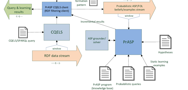
Currently there are two clients: 1) a console client, where the stream data is entered manually in the console in ASP/PrASP syntax (mainly for testing and debugging purposes) and 2) an RDF/SPARQL streaming client (PrASP CQELS client) which employs the Linked data stream processing engine CQELS [46]. This way, PrASP can be used as a tools for uncertainty reasoning about RDF streams (that is, about results of CQELS queries), whereas the console client can be seen as a simple REPL for PrASP (although the PrASP Web Interface (Sect. 2) might be easier to use for trying out PrASP).
The console client is located in directory PrASP_StreamConsole.
The stream client (PrASP CQELS client) is located in directory PrASP_RDF_StreamClient.
1) To use the PrASP Console Client (folder prasp_StreamConsole), first start PrASP as usual, but specify additional argument --stream 7777 (or some other port number which must match the port number specified in the PrASP Console Client script). PrASP expects all the usual files at startup - if you want it to start without initial background knowledge or initial learning examples, you need to provide an empty .prasp (or an empty .examples file, respectively).
As soon as PrASP shows ”Listening for stream data …”, start the console client using \prasp_cc.sh (Linux, MacOSX) or \prasp_cc.bat (Windows)
Now you can send new beliefs or examples to PrASP by typing after "> ". Beliefs are incrementally added to the initial background knowledge (i.e., given by the .prasp-file specified when PrASP was launched).
Sending examples only make sense if you started PrASP in learning mode, i.e., using
a .hypoth and an possibly empty .examples file. Sending examples and beliefs can also be mixed.
E.g., send a fact (belief) by entering B coin2(heads). (always conclude formulas with a “dot”.)
Send an uncertain belief using, e.g., B [0.7] coin2(heads).
(You can also send certain and uncertain rules, negative formulas, conditional probabilities, etc. as beliefs.)
Send an example using, e.g., E coin2(heads).
After each step, PrASP replies with updated results (query results or re-weighted hypotheses). Enter an empty line to see the current query results.
Optionally, you can specify the lifetime of a formula using a number directly behind ”B” or ”E”.
E.g. B10 [0.7] coin(heads). means that formula coin(heads) remains in the KB only during a time window consisting of the next 10 steps and is then removed. A “step” is a single interaction with PrASP , but for the calculation of formula lifetime only those steps count where a belief or example was added.
If omitted, life expectancy is infinite. If you always use the same number, you have a window.
Formulas can also be retracted, using RB f (retract a belief) or RE f (retracts an example). All formulas need to be concluded by a dot, as usual. Note that it is only possible to retracts formula which have been added before using the client, not formulas
in the KB file (the .prasp-file) or in the examples file provided at PrASP startup.
Commands SB and SE show the list of currently valid external beliefs or examples, respectively.
2) PrASP CQELS client, for supplying PrASP with a filtered stream (results of a SPARQL/CQELS [46] query) which itself originates from an RDF data stream:
This client is located in folder prasp_RDF_StreamClient.
First, edit prasp_rdfsc.sh or prasp_rdfsc.bat in order to specify data files, home directory (where CQELS should put cache files etc), data URIs, and the file with the extended CQELS-like query (e.g., query1.psquery).
Then, start PrASP as usual, but specify additional argument --stream 7777 (or some other port number, as defined in \prasp_rdfsc).
Example (using the “floorplan” example files in folder \prasp_RDF_StreamClient):
prasp floorplan.examples floorplan.prasp floorplan.hypoth --folconv none
--mod1 --noautoindeps --noindepconstrs --cacheinfsetup --stream 7777
Instead of this command-line, you can specify any other switches and tasks, e.g., inference instead of learning. The only difference compared to a normal PrASP invocation is argument --stream 7777 (and optionally --cacheinfsetup).
As soon as PrASP shows ”Listening for stream data …”, start the client using .\prasp_rdfsc.sh or prasp_rdfsc.bat
Note that floorplan.examples is empty (but it still needs to be provided).
In addition to the usual PrASP files, you also need an extended CQELS/SPARQL-like query file (file ending .psquery):
This file needs to be specified using set QUERY=... within prasp_rdfsc.sh/.bat. It provides the SPARQL-like query pattern for the CQELS-based client and should not be confused with the .query file necessary to specify inference queries (which you need additionally if you want to use the streaming data for inference instead of learning).
The transformation pattern SPARQL-Result(Pr)ASP facts is specified directly
inside the CQELS SPARQL-like query, after keyword PrASP :
...
SELECT ...
PrASP pattern [OMIT URIs]
...
At this, pattern is the same as for the console client, e.g.,
E20 detectedAt(?person, ?loc, TIMESTAMP). (don’t forget the dot).
Any ?vars in pattern need also to occur after SELECT. TIMESTAMP is an automated counter 1, 2,…
[OMIT URIs] specifies that the listed URIs (separated by commas) shall be omitted in the ASP formulas.
[OMIT URIs] and use of TIMESTAMP are optional.
An example query file is provides as query1.psquery
Reasoning about streams might profit significantly from PrASP command-line switch --cacheinfsetup in case the stream contains repeated subsequences.
For details about the pure CQELS query syntax (without PrASP extensions), please consult [46].
(More tbw.)
3.13 Performance tuning
PrASP ’s default settings are rather conservative. This section shows how to increase inference (and indirectly learning) speed using problem-specific command-line options. But foremost, the background knowledge influences inference performance - while PrASP ’s input language is quite expressive, not all valid probabilistic logic programs and query types are likewise suitable for fast or even just tractable inference.
3.13.1 A rule of thumb
The number of options available in PrASP can appear a bit overwhelming at first. Here’s a rule of thumb which proved to be a good heuristic in many of our own experiments:
- 1.
-
2.
Firstly, invoke PrASP with the default (“vanilla”) settings. Try different solvers using --linsolveconf.
-
3.
If this turns out to be too slow, try next with --itrefinement --models 0. Given a full set of models (enforced with --models 0), this will still give you an accurate result (modulo round-off errors).
-
4.
As further measure, let PrASP try simplifying the problem using --mod1 (together with --folconv none, if possible).
-
5.
In some cases, neither default settings nor --itrefinement are useful due to the complexity of the problem. Use --simanneal (in combination with --nosolve) to approach such problems.
-
6.
There is a pretty large number of other command-line switches and arguments which have an influence on inference speed. They are detailed further below in this section and in Section 6.3.
-
7.
Since version 0.9, PrASP also supports MaxWalkSat as inference algorithm (see --maxwalksat), which turns PrASP into a sort-of-Markov-Logic MAP inference tool (however, this restricts the sort of formulas you are able to use in your background knowledge and queries).
3.13.2 Motivation
To obtain a deeper understanding of performance issues and their causes, let’s take a look at the parameterized coins example again:
coin(1..20).

#indep
[0.6] coin_out(1,heads).
[[0.5]] coin_out(N,heads) :- coin(N), N != 1.
#endIndep

1{coin_out(N,heads), coin_out(N,tails)}1 :- coin(N).

n_win :- coin_out(N,tails), coin(N).
win :- not n_win.
Even with only 20 coins, inference using default “vanilla” settings (linear system solving) is slow: all coin tosses are independent from each other, which causes a combinatorial explosion of possible worlds - we get 1048576 possible worlds and accordingly
the same number of rows in the equation system we would need to solve. However, the real bottleneck here is not so much the linear system solving step (PrASP’s native LAPACK solver can compute the solution for systems with variables/possible worlds in a few seconds on contemporary single CPUs) but the time required to generate possible worlds.
Generally, the more weight-annotated formulas and other choices (disjunctions) a spanning program contains, the larger the number of possible worlds (stable models, answer sets), and the more time is required for inference and learning.
However, there are a number of approaches built into PrASP which cope much better with larger systems than the “vanilla” setup:
3.13.3 Use of Clingo 4 and remote sampling
This implementation of some of the model generation and sampling methods is typically
much faster than older Gringo 3/Lparse based approach.
However, it requires you to use Gringo and Clingo version 4 or higher, which has a number of consequences for PrASP program syntax. See --noremotesampling for details. This switch actually deactivates Clingo 4-based remote (i.e., fast) model generation, but also provides some background information about it. To activate remote sampling, you just need to install Gringo 4 & Clingo 4 and to make sure that PrASP finds them in the PrASP directory (see Section 2).
The only required change to the coins-example program above would be to replace the comma with a semicolon within 1{coin_out(N,heads), coin_out(N,tails)}1 :- coin(N), in order to meet Gringo 4 syntax requirements.
However, with the coins example above, inference would be still slow with this measure alone. For this particular example, e.g., simulated annealing (see below) in combination with --nosolve (to omit the linear system solving step) and --noindepconstrs --noautoindeps (to omit the generation of independence constraints) would be an appropriate and fast approximation approach.
3.13.4 Iterative refinement as inference algorithm
Another approximate inference method for medium-size or large systems is iterative refinement (switch --itrefinement). Please see Sect. 5.6 for details.
3.13.5 Simulated annealing as inference algorithm
With --simanneal, PrASP uses a variant of simulated annealing for approximative inference. For problems with many degrees of freedom (large number of uncertain formulas in background knowledge), this approach (see Sect. 5.3) is typically faster compared to the default approach for medium-size or large systems. --simanneal also copes better than --itrefinement with small numbers of models. It is often the only way to approach complex systems for which no accurate solution can be found.
Simulated annealing works often much faster for such large systems compared to the default inference approach, however, it does not necessarily discover the best solution (the one with maximum entropy). Also, consideration of formula independence is a tricky issue: in some cases, independence speeds up the algorithm, in other situations it slows it down (details below).
Random sample models are computed until the probability distribution over all sampled models matches the probabilities (formula weights) specified in the background knowledge. With --simanneal, the equation solving phase is not required (and therefore --simanneal is typically used in connection with --nosolve). However, in some cases, it might make sense to omit --nosolve - in that case --simanneal works as a possible world sample generator and the probability distribution over the sampled possible worlds is computed using equation solving, which can lead to increased accuracy (at the price of being much slower than --nosolve unless the system is very small).
--simanneal can optionally be configured using various parameters which have a tremendous influence on computation time and accuracy of results - please see 6.3 for details.
Also various command-line switches have a strong influence on how simulated annealing behaves, such as --unisample, --ascheckmode, --mod1 and --noindepconstrs. Typical combinations
are achieved with -o2 or -o2asp.
Tips:
-
•
--simanneal performs a complex multi-goal optimization task. It works best if there are no or only few conditional probabilities specified in background knowledge (as these generate an large set of candidate samples) and if known mutual or pairwise independence constraints are not considered (--noindepconstrs). --simanneal can still make use of independence assumptions if --noindepconstrs is provided, PrASP just doesn’t generate additional constraints then besides the weighted formulas in background knowledge.
Also, all involved formulas should ideally be in ASP syntax and --folconv none should be set. --simanneal works with other settings too, but significantly slower. -
•
Ideally, all weighted formulas should be mutually independent (as in ProbLog [12]). In that case, the algorithm can typically compute the result in a single step. This does not contradict the previous advice (to specify --noindepconstrs), since --noindepconstrs only prevents the generation of independence enforcing constraints but not the assumption of independence.
-
•
Annotated formulas in background knowledge, query formulas, learning examples and hypotheses should ideally be so-called simple formulas, see 3.13.8. Again, this is not mandatory, but it speeds up PrASP significantly. If this is not possible, consider specifying a different model checking approach using --ascheckmode in case the number of models of the spanning program is very large (see below).
-
•
--simanneal can be combined with other optimization approaches (e.g., --mod1).
-
•
Although --simanneal can be used with --intervalresults, this combination has its issues (see 3.5).
-
•
The “energy” parameter of --simanneal specifies the acceptable euclidean distance (which PrASP aims to minimize) between the vectors of actual and specified probabilities of uncertain formulas in background knowledge, given the current list of sampled models of the spanning program. A larger “energy” argument means less accurate (but quicker) results. Further details can be found in Sect. 5.3.
3.13.6 Using alternative approaches to checking of formula validity
At various points, PrASP needs to check whether a formula holds in a certain possible world . The obvious approach to this is to check if the given possible world is an element of the enumeration of all possible worlds of the given formula in conjunction with the spanning program. There are two ways to make this faster: 1) use simple formulas (see 3.13.8) for which PrASP can check if they hold in a given model without the need to call the ASP solver and/or 2) enforce a different model checking approach using command-line switch --ascheckmode (but by default, PrASP typically uses a fast approach here already).
There is also the possibility to restrict the number of models requested from the ASP solver using --models n, however, even though these can be sampled near-uniformly, there is no guarantee that results are correct using these samples.
3.13.7 Combining and filtering background knowledge formulas
--mod0
Using --mod0, PrASP combines unweighted ground ASP rules (except for headless rules) which have the same head and whose bodies consist of independent sets of ground literals only, and replaces them with weighted formulas. See Sect. 4.7 for how to declare such independence. To obtain a speed gain, a significant number of rules suitable for simplification has to exist in the PrASP program. If this is not the case, --mod0 slows down inference. Weighted formulas with single-bracket weight annotations in background knowledge need to be ground for --mod0 to work.
--mod0 can be combined with --mod1 (which is explained below). This allows PrASP to remove independent formulas from the background knowledge in case these have only been used within rule bodies which have been simplified using --mod0.
Also see --limitindepcombs in Section 6.3 and the general explanation of how PrASP deals
with probabilistic independence in #indep...#endIndep (under meta-statement #indep).
Provide switch --verbose for information about which rules couldn’t be simplified by PrASP , and why.
Observe that PrASP generally only simplifies formulas in background knowledge, not any formulas in query files (at least not beyond any query simplifications performed by the ASP grounder).
--mod0 doesn’t yet support full Gringo 4 syntax.
--mod1
With --mod1 (which can be used alone or together with --mod0), PrASP analyses the background knowledge and removes all parts on which the result of the queries cannot depend. The speed gain depends on the respective .prasp program and can be either tremendous (if the query depends only on a small module of the background knowledge), or moderate, or even negative (if the cost for the dependency analysis prevails the gain from the modification). For the coin flipping example above, the speed gain is still about 50%, even though query win depends on all 13 coins (the reason for this is that --mod1 removes facts coin(1), coin(2), etc at some stage of the process).
--mod1 has shortcomings too: 1) weighted formulas with single-bracket weight annotations in background knowledge need to be ground (this is typically not a severe restriction).
2) All query formulas are converted into sets of grounded formulas. Multiple ground instances are shown in #{...}# -brackets in query results.
3) --mod1 together with conditional probabilities in background knowledge might lead to errors or inaccuracies (PrASP therefore shows a warning if --mod1 is used and such formulas are found in the .prasp file)171717If the spanning formula generated for the conditional probability conveys all information necessary for the dependency analysis performed by --mod1, there is no problem. But PrASP cannot guarantee this and therefore warns against combining --mod1 with conditional formulas in background knowledge.. For conditional probabilities within query files, there is no such issue.
4) Finally, analyzing and optimizing a program using --mod1 takes time itself which needs to be traded off against the speed gain obtained with the automatically optimized program.
Observe that --mod1 prunes a program and can thus turn a logically inconsistent program into a consistent one (which is normally not desired) by removing parts on which no query depends.
Since --mod1 and other (internal) optimization approaches use the information found in query-files in order to determine which parts of the background knowledge are relevant, it can make sense to put different query formulas into different query-files: for each --query-occurrence in the command-line, and for each file with file name ending .query which is not bound by any other argument, the background knowledge is processed anew (so that different query-dependent optimizations can be applied). In contrast, for each set of query files bound by a certain --query in the command-line, PrASP applies the same optimizations to the background knowledge and the actual inference task.
3.13.8 Using “simple formulas”
PrASP deals with formulas which are plain ASP rules or conjunctions which consist of ground literals only considerably faster
than with other kinds of formulas, because the models of such formulas can be computed relatively easily.
It is recommended to use such simple formulas whenever possible, as they speed up inference and learning without
sacrificing much expressiveness (many probabilistic logics can deal only with even simpler formula classes). Other types of formulas can still be used to, provided they are translated into “simple” format during grounding phase (e.g., by annotating them with double-square weights, although this only guarantees grounding).
Benefits of using simple formulas apply to all kinds of input (including background knowledge and queries), even if only some formulas are in this format, there is already a speed gain.
PrASP recognizes formulas of the syntactic forms a1 & a2 & ... & an or n#count{a1,a2,...,an}n or n{a1,a2,...,an}n as simple formulas if all ai are ground literals, and also combinations thereof. Also, ASP rules of the forms
a1 :- a2, ... ,an and :- a2, ... ,an are “simple formulas” if all ai are ground literals. From a purely syntactical point of view, “simple rules” are thus similar to ground Datalog rules.
3.13.9 Disabling full FOL syntax
Another means to increase speed which is applicable alone or in combination with most other command-line options is to disable the FOLASP converter by specifying
--folconv none. Of course, all formulas need to be in ASP syntax then. For the coins example, we can achieve this simply by replacing [?] not win with [?] :- win in the queries file.
3.13.10 Disabling independence enforcement constraints ot automatic detection of independence
For known (declared or automatically discovered) mutually or pairwise independent sets of events (propositions), PrASP generates certain constraints. While these constraints can speed up PrASP in some cases (e.g., 3.13.7), in other cases they can slow down inference and learning. To disable them entirely, use switch --noindepconstrs. To disable them for event combinations of certain lengths only, use --limitindepcombs (6.3).
Note that --noindepconstrs has no influence on
whether or not formulas are treated as independent in other contexts - e.g., --mod0 can still make use
of independence declarations even if --noindepconstrs is provided.
--noautoindeps omits the automated search for a (globally) mutually independent set of atoms. In case you have specified all independent formulas in the background knowledge file (see Section 4.7), --noautoindeps does not only lead to faster inference but it also avoids the potential problem that the automated identification erroneously misidentifies some atom.
Even without speed considerations, it is a good idea to declare independence explicitly using the means described in 4.7 and to deactivate automatic discovery, since the latter relies on grounder-dependent heuristics which does not always work as expected.
3.13.11 Answering queries using mere initial sampling and --nosolve
See Sect. 3.8
3.13.12 Using PrASP for plain ASP reasoning
PrASP subsumes plain ASP reasoning about non-probabilistic knowledge. Besides generating answer sets (--pwsamples), it adds a query facility to ASP. E.g., using the following program:
flies(X) :- bird(X), not ab(X).
bird(tweety).
bird(sam).

bird(X) :- penguin(X).
ab(X) :- penguin(X).
penguin(sam).
…queries such as [?] flies(tweety) or [?] 2{flies(sam),bird(sam)}2 can be used to compute truth values (represented by 1 and 0) for these formulas, provided the answer sets are in agreement about them (otherwise you would of course get probabilities other than 0 and 1, e.g., when you replace penguin(sam) with 0{penguin(sam)}1).
However, these results are still computed with the help of probabilistic inference, which has two not-so-nice consequences: 1) there is a certain time overhead involved compared to a direct call of the ASP grounder/solver, and 2) due to round-off errors, you might sometimes get in fact, e.g., 0.999999999 instead of 1.
3.13.13 Further means to speed up inference and learning
- Grounding of non-ground formulas can take up a significant amount of time, even with a fast grounder such as Gringo. PrASP the following options and meta-statements for influencing the grounding process:
- •
-
•
#dontExternalize..#endDontExternalize(see Sect. 4.7) -
•
#external(via Lparse/Gringo)
- If --mod1 is specified (or an optimization switch which comprises --mod1), those parts of the background knowledge are removed on which no query formulas depend. It follows that the number of query formulas per query task should be kept to a minimum then. On the other hand, the probability distribution computed without --mod1 is reused for multiple different query formulas, i.e., in this case it is better to solve all query formulas at once.
- Significance speed improvements in repeated similar inference and learning tasks can be achieved using command-line switch --cacheinfsetup provided the task comprises some repetition (e.g., repeated floating windows in stream reasoning). It needs to be used with care though, since the cache controller makes the assumption that all inferencer setups are identical.
- If the user already knows a suitable estimation of the required number of initial sampled models, this number should be provided using --models instead of letting PrASP figure out a number heuristically (or, even worse, use all models of the spanning program). Estimating the number of models of the spanning program is a costly task and not very precise.
- Switch --ignoreentropy --ndistrs 1 make PrASP compute probability distributions somewhat faster if the default inference approach is being used (which is generally rather slow unless for very small systems) (see 3.5).
- Switch --checkconsistency slows down inference significantly.
- Learning becomes a little faster with switch --nonorm, which deactivates a result normalization step. With --nonorm, hypotheses weights are shown as computed by the parameter estimation algorithm, even in case these weights are probabilistically inconsistent in the context of the background knowledge. Otherwise, a normalization step aims for leveling out such inconsistencies.
- Most of the considerations before also apply to learning (Section 3.11), since learning is based on inference.
In the particular case of our coins-example (but not in general!), we can obtain an approximation of the correct inference results using --models n, where
n is the approximate number of possible worlds PrASP should compute. For 13 coins, we obtain results which are fairly accurate for n 4000. However, --models is in general not a valid optimization approach since it is virtually impossible to predict whether the sampled models are sufficient input
for the equation solver so that the resulting probability distribution over possible worlds is accurate enough. A better approach to sampling (embedded in an optimization task) is via simulated annealing (command-line
option --simannealing).
- Finally, using a different grounder/solver can make a difference. E.g., using Windows,
--groundersolver gringoThenClaspMT.bat
"-n%NZNUM --verbose=1 --project"
"--project --rand-freq=0.9 --sign-def=3 --seed %SEED"
specifies that a multithreaded version of Clasp 2/3 should be used (see script gringoThenClaspMT.bat for details).
4 Syntax
4.1 ASP and FOL syntax
The syntax of ASP formulas without their weights corresponds mostly to the input syntax of the grounder. The default grounder is Gringo [36] - please see the Gringo/Clingo manual [37] for a detailed description of the input language. Observe that Gringo/Clingo 3 and Gringo/Clingo 4 differ significantly wrt. input syntax.
If the optional FOLASP converter F2LP is installed or the internal FOLASP converter is specified (see switch --folconv), formulas can alternatively be in FOL syntax as specified for F2LP (see [3]). Within the same file, formulas of both types (ASP and FOL/F2LP) can occur, however, ASP and FOL syntax should not be mixed within the same formula (although there is some support for ASP constructs such as aggregates within FOL formulas if you use F2LP).
Syntax restrictions are listed in Sect. 7. In particular, a single formula currently cannot extend over more than one line of text.
Irrespectively of the specific grounder or FOL converter being used, PrASP supports quoted "strings" and 'strings' in term positions. Because ASP grounders typically don’t support strings directly, PrASP translates them into certain constants (names consisting of alphanumeric characters or underscores) and thus strings can be used with those built-in predicates provided by the ASP grounder which work with constants (see grounder manual). The translation from strings to constants preserves string equality and lexicographic order of strings. E.g., "abc" < "xyz" holds, using Gringo 3 as grounder.
Within strings, escape sequences can occur (e.g., "abc\ndef"). In addition to the usual characters that need to be escaped (like newline),
it is also required to escape character ’%’. E.g., you need to write "abc\%xyz" instead of "abc%xyz".
The full syntax of string literals and the list of supported escape sequences (except the handling of ’%’) can be found in
http://www.ecma-international.org/ecma-262/5.1/#sec-7.8.4
The other kinds of literals which are supported in term positions are integer numbers and alphanumeric constants.
More tbw.
4.2 Comments
Single-line comments are prefixed by %. Multi-line comments need to be enclosed in %*...*%. Example:
[0.05] a & b.  % a single-line comment
%* This is
a multiline
comment. *%
4.3 Parsing order
The sequence of background knowledge parsing and preprocessing steps performed by PrASP is depicted in Figure 2. The sequence for processing query and other types of files is similar, but of course without generation of a spanning program (Sections 5.1,4.5).
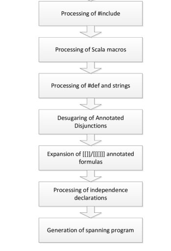
4.4 Formula annotations and weights
In principle, any ASP or FOL formula can be annotated with a probability. Such weight annotations in background knowledge (.prasp files) can take the syntactic forms listed below. In query and hypothesis files, annotation syntax is similar, with the difference that numerical weights need to be replaced with ? and that computed weights (see below) are not allowed. In .example files, no annotations are allowed.
Terminology: an expression of the form [W] or [[W]] or [[[W]]] in front of a plain ASP or FOL formula is called annotation (of ).
If W is a single number between 0 and 1 (inclusively) or consists of two such numbers separated by a semicolon (the second one larger than or equal to the first), W is called the weight of the formula. W then directly represents either a point probability (in case W is a single number) or an interval of probabilities (if W has the form wx;wy). A weight of the form wx;wy is called probability interval.
If W is an expression of the form w|c where c is a formula and w is either a single number or an interval as defined above, the annotation is called a conditional probability annotation. In that case, the weight specifies .
The annotated formula is called a weighted formula. If the weight is neither 1 or 1;1, the formula is also called uncertain.
If W is ? or ?|c, the formula is called query formula (or query).
In addition to these, some other types of annotations exist. Full list of formula annotations:
- [w] f
-
where is a number between 0 and 1 which represents the marginal probability of formula . can be ground or non-ground (containing variables). can be either in ASP- or in FOL/F2LP-syntax.
A few examples for well-formed PrASP formulas with non-conditional point probabilities as weights:
 [0.3] a.

 [0.7] :- a.

 [0.7] not a.

 [0.1562] a & (b | c) & d -> e | f & not g.

 [0.5] heads(coin(3)).

 [0.9] heads(X) :- coin(X), not lose.

 heads(X) :- coin(X), not lose.  % same semantics as previous formula

 [.3] heads(X) | tails(X) :- coin(X), X < 4.  % But note that non-ground
 % formulas are usually annotated with other forms of weights, see further
 % below in this section.

 [0.95] ![A,B]: (foo(A) | bar(B)) -> fooBar(A,B).

 [0.01] ?[X]: foo(X) & bar(X).

 [0.615] 2#count{coin_out(N,heads):coin(N)}5.

 [0.6] 1#sum{coin_out(N,heads):coin(N)}10 | v(X) :- not q(X,Y).
In these examples, each probability refers to the respective formula in toto (that is, a single probability weights the entire expansion of this formula into a set of ground formulas), not to each ground instance individually. If, for example, the domain of variable
Xis ,[0.5] p(X)declares that the probability of is 0.5, which is generally not the same as . If you want to let the weight refer to individual groundings ofp(X), use one of the multi-bracket annotations instead, as explained below. Sect. 3.6 contains more details about how PrASP deals with non-ground formulas. - [[w]] f
-
where is a number between 0 and 1 which represents the marginal probability of each ground instance of non-ground formula 181818If is ground, [[w]] f has the same meaning as [w] f.. A unique index of each and the total number of ground instances is available in as
#INDEXand#NUMBER, respectively. These pseudo-variables are mainly useful in regards to computed weights of the form [[pred]] f (see further below) where a more detailed explanation is provided.Note (1): the order of the generated ground instances is determined by the grounding algorithm and some post-processing (multi-token lexicographic sorting of ground formulas). It can be influenced using --groundingconf.
Note (2): the ground instances of [[w]] f are generated either locally by PrASP itself (internal grounding) or by the external ASP grounder which might apply simplifications. Again this can be influenced using --groundingconf. In the latter case, the result of the [[w]] f expansion comprises only formulas and formula parts which are not simplified away by the grounder, given the so-called grounding precontext (see Section 4.6).
The grounding precontext is added to formula
fwhen it is grounded by an external grounder. It consists of the entire file except annotated formulas and PrASP meta-statements. Furthermore, with Gringo or Lparse as grounder, it contains automatically generated#externalstatements for all predicates found within facts or heads of rules of annotated non-query formulas, in order to protect these from being simplified away by the grounder (since their truth values are naturally not known yet at this point). If you don’t want#externalstatements to be generated, surround the respective annotated formulas with#dontExternalize...#endDontExternalize191919It is also possible to put #external statements manually into PrASP programs, e.g., to selectively protect certain predicates. In combination with #dontExternalize this gives you full control over the externalization of predicates. Yet another option is to use switch --keep-facts with Gringo 4. See --groundingconf for how to pass options to the grounder.
Also, if an external grounder is being used, PrASP pools and grounds all formulas annotated with[[...]]using a single external grounder call, provided the annotated formulas don’t require special treatment (e.g., in case of symbolic weights) and they are not grounded internally.For non-background knowledge files (such as
.query-files), the grounding precontext also includes all non-annotated formulas and non-PrASP meta-statements (such as#domainstatements or Lua- or Python-script) in the background knowledge file (this behavior can be deactivated using
--groundingconf).Note (3) For formulas where grounding is performed internally by PrASP , no grounding precontext is added to
f, however, the grounding precontext is used to determine the domains of ASP variables. In this case PrASP still calls the external grounder at one point, in order to determine the set of all ground atoms in the context. --groundingconf allows you to change this default behavior so that only ground atoms are considered for variable domains which are explicitly provided (such aspeople(mary;john;anna)), avoiding the external grounder call.Note (4): All variables in [[w]] f should be bound by domain predicates in the grounding precontext (predicates which can be fully evaluated during grounding). This is not a strict rule, but adhering to it avoids hard to detect grounding errors due to incorrectly bound variables.
Note (5): In the specific context of
[[..]]and[[[...]]]also formulas with intervals (..) which expand to two or more formulas by grounding count as “non-ground”, even if they don’t contain variables.
E.g.,[[0.5]] twoCoins(1..3,1..2)expands to[0.5] twoCoins(1,1),[0.5] twoCoins(1,2),[0.5] twoCoins(2,1), etc.The above notes apply to background knowledge as well as to queries and other files in which
[[...]]can occur, and analogously also to formulas annotated with[[[...]]](see below).Remark: unannotated or single-square annotated non-ground formulas such as
[0.8] asthma(P) :- smokes(P), person(P)eventually need to be grounded too, but this happens at a different stage of inference, namely when we check if formulas have certain models. In contrast to[[...]], their respective weight does not refer to each individual ground instance but to the entire formula (conjunction of ground instances in case of an ASP formula).Here is a complete example for the correct use of
[[...]]:person(1..3). [0.2] smokes(1). [0.3] smokes(2). smokes(3). [[0.8]] asthma(P) :- smokes(P), person(P).
In this example, variable
Pis correctly bound by predicateperson/1.On the other hand, the following code is erroneous under the assumption that we intend to compute the probability of having asthma from smoking:
person(1..3).
[0.2] smokes(1).
[0.3] smokes(2).
smokes(3).
[[0.8]] asthma(P) :- smokes(P).
While syntactically correct, the above PrASP program would give unexpected results since
Pis not bound by any domain predicate.Pis bound by predicatesmokes, however,smokesis not a domain predicate (since it cannot be fully evaluated during grounding).Simplification of ground instances can be influenced using switch --groundingconf, however, this option should be used with care.
It is a good idea to take a look at the resulting expansion into weighted ground instances of the original formulas using --showexpansion if unsure about which ground formulas are actually generated.
Further examples:
Example (1):
coin(1).
coin(2).
coin(3).

[[0.5]] heads(X) :- coin(X).
…expands to
coin(1).
coin(2).
coin(3).

[0.5] heads(3) :- coin(3).
[0.5] heads(2) :- coin(2).
[0.5] heads(1) :- coin(1).
…which is automatically simplified202020PrASP fully supports probabilistic rules, but in the example above, the ASP grounder removes the :- coin(_) parts as redundancies (they are only required to determine the domain of variable X and not needed anymore after grounding since they are equivalent to true in the three example rules). to
[0.5] heads(3).
[0.5] heads(2).
[0.5] heads(1).
Example (2):
dice(1..2).
face(1..6).

[[0.7]] foo(D,F) & bar(#INDEX) & total(#NUMBER) <-  dice(D) & face(F).
…expands to (using Gringo 4212121Note that we would get a different order of ground instances using Gringo 3. ):
dice(1..2).
face(1..6).

[0.7] 3{foo(1,1);bar(1);total(12)}3.
[0.7] 3{foo(1,2);bar(2);total(12)}3.
[0.7] 3{foo(1,3);bar(3);total(12)}3.
[0.7] 3{foo(1,4);bar(4);total(12)}3.
[0.7] 3{foo(1,5);bar(5);total(12)}3.
[0.7] 3{foo(1,6);bar(6);total(12)}3.
[0.7] 3{foo(2,1);bar(7);total(12)}3.
[0.7] 3{foo(2,2);bar(8);total(12)}3.
[0.7] 3{foo(2,3);bar(9);total(12)}3.
[0.7] 3{foo(2,4);bar(10);total(12)}3.
[0.7] 3{foo(2,5);bar(11);total(12)}3.
[0.7] 3{foo(2,6);bar(12);total(12)}3.
Example (3) - see Sect. 3.10 for details:
friend(a,b).
friend(b,c).

#dontExternalize
[[0.7]] influences(X, Y) :- friend(X, Y).
#endDontExternalize

influences(X, Y) :- influences(X, Z), influences(Z, Y).
To expand a non-probabilistic non-ground formula to its ground instances, annotate it with weight
[[1]]. But notice that this is not required to handle non-ground formulas. Example:person(a;b;c). #domain person(X). #domain person(Y). [[1]] friend(X,Y).
expands to
[1] friend(a,a).
[1] friend(a,b).
[1] friend(a,c).
[1] friend(b,a).
[1] friend(b,b).
[1] friend(b,c).
[1] friend(c,a).
[1] friend(c,b).
[1] friend(c,c).
With the program above you would obtain the same query results as with the following PrASP program:
person(a;b;c).

#domain person(X).
#domain person(Y).

friend(X,Y).
The only difference here is that the latter program is not grounded by PrASP itself. PrASP rather checks for each stable model (there is only one) whether the non-ground formula holds in that model (however, to check this, the external grounder needs to ground
friend(X,Y)). In contrast, with the second program, PrASP first groundsfriend(X,Y)and later checks for each ground instance whether it holds in the only stable model (which is the same as the stable model of the second program). - [w|c] f
-
where is a number between 0 and 1 which represents conditional probability . and are formulas (ground or non-ground).
Example (1):
coin(1).
coin(2).
coin(3).

[0.8|heads(X) :- coin(X)] win :- coin(X).
Example (2), which shows that conditions can also be rules (although in practice they are typically (ground) facts):
[0.3|D <= 2 :- dice(D)] faceObserved(F) :- face(F).
- [[w]] condProb(f,c) :- b
-
where is a number between 0 and 1 which represents conditional probability for any pair of corresponding ground instances , of atomic formulas and such that holds and can be evaluated during grounding.
condProbis a reserved keyword in PrASP which is treated by the ASP grounder as a predicate although it is actually just a means to combine and in one formula.
The purpose of this syntax is to generate the list of all groundings of where the variables in and are restricted using some expression which affects both and . Groundings of conditional probabilities can also be generated using[[w|c]] for[[[w|c]]] f(see below), however, there the two formulas and are expanded separately from each other.The statement about the grounding-context for [[w]] f above also applies here (and other
[[...]]/[[[...]]]style annotated formulas).Both and must be atomic formulas here. Observe the double square brackets around the weight.
To see the result of the expansion, use command-line switch --showexpansion.
Example (Gringo3/Lparse version):
x(1..3).
#domain x(I).
#domain x(J).
#domain x(K).
[[0.3]] c(K).
[[0.5]] condPr(h(I,J),c(K)) :- J == K.
The annotated formulas above expand to
[0.3] c(1).
[0.3] c(2).
[0.3] c(3).

[0.5|c(3)] h(1,3).
[0.5|c(2)] h(1,2).
[0.5|c(1)] h(2,1).
[0.5|c(3)] h(3,3).
[0.5|c(2)] h(2,2).
[0.5|c(2)] h(3,2).
[0.5|c(1)] h(1,1).
[0.5|c(1)] h(3,1).
[0.5|c(3)] h(2,3).
Alternatively, we can encode this example as follows. This version works with both Gringo3 and Gringo4 (since it doesn’t use
#domain):x(1..3). [[0.3]] c(K). [[0.5]] condPr(h(I,J),c(K)) :- J == K, x(I), x(J), x(K).
- [[w|c]] f
-
where is a number between 0 and 1 which represents conditional probability for any pair of corresponding ground instances , of formulas and . and correspond if they have the same position in the sequence of ground instances returned by the ASP grounder for or , respectively. The number of ground instances of and must be identical.
Exception: if is the only ground instance of , the pairings are .Both and can be any formulas, including rules.
Observe that if is a rule, the rule body doesn’t affect . So, in order to restrict the groundings using some boolean expression (in form of a rule body which can be resolved during grounding), this body needs to be present in as well as . See Example (3) below. Where this is not possible, use the
condProb(f,c) :- bsyntax instead (see above).The statement about the grounding-context for [[w]] f above also applies here (and other
[[...]]/[[[...]]]style annotated formulas).To see the result of the expansion, use command-line switch --showexpansion.
Example 1 (Gringo3/Lparse-version):
person(1..3).

#domain person(P).

[[0.3|smokes(P)]] asthma(P).

[0.1] smokes(1).
smokes(2).
[0.85] smokes(3).
Example 1 (Gringo4/ASP language standard-version):
person(1..3).

[[0.3|smokes(P) :- person(P)]] asthma(P) :- person(P).

[0.1] smokes(1).
smokes(2).
[0.85] smokes(3).
Example 1 expands to
[0.3|smokes(1)] asthma(1).
[0.3|smokes(2)] asthma(2).
[0.3|smokes(3)] asthma(3).
...
Example (2):
person(1).
person(2).
person(3).

[[0.3|smokes(P) :- person(P)]] some_asthma.
…expands to
[0.3|smokes(1)] some_asthma.
[0.3|smokes(2)] some_asthma.
[0.3|smokes(3)] some_asthma.
Example (3):
person(1).
person(2).
person(3).

[[0.3|smokes(P) :- person(P), P != 2]] asthma(P) :- person(P), P != 2.
…expands to
person(1).
person(2).
person(3).

[0.3|smokes(1)] asthma(1).
[0.3|smokes(3)] asthma(3).
- [[[w|c]]] f
-
where is a number between 0 and 1 which represents conditional probability of any combination of ground instances , of formulas and .
Observe that if is a rule, the rule body of doesn’t affect . So, in order to restrict the groundings using some boolean expression (in form of a rule body which can be resolved during grounding), this body needs to be present in as well as . See Example (2) below. Where this is not possible, consider using the
condProb(f,c) :- bsyntax instead (where possible, see above).The statement about the grounding-context for [[w]] f above also applies here (and other
[[...]]/[[[...]]]style annotated formulas).To see the result of the expansion, use command-line switch --showexpansion.
Example:
person(1).
person(2).
person(3).
#domain person(P).

[[[0.3|smokes(P)]]] asthma(P).
…expands to
[0.3|smokes(3)] asthma(3).
[0.3|smokes(2)] asthma(3).
[0.3|smokes(1)] asthma(3).
[0.3|smokes(3)] asthma(2).
[0.3|smokes(2)] asthma(2).
[0.3|smokes(1)] asthma(2).
[0.3|smokes(3)] asthma(1).
[0.3|smokes(2)] asthma(1).
[0.3|smokes(1)] asthma(1).
Example (2):
person(1).
person(2).
person(3).

[[[0.3|smokes(P) :- person(P), P != 2]]] asthma(P) :- person(P), P != 2.
…expands to
person(1).
person(2).
person(3).

[0.3|smokes(1)] asthma(1).
[0.3|smokes(3)] asthma(1).
[0.3|smokes(1)] asthma(3).
[0.3|smokes(3)] asthma(3).
(…which is probably not very useful, but exemplifies the difference to the effect of using double square brackets or
condProb.) - [pred] f
-
where pred is the predicate name of an unary atom which occurs in formula . The meaning is as that of the corresponding form with a numerical literal as weight, however, here the numerical weight is computed (taken from the argument of pred computed during the grounding phase). In others words, this syntax allows for computed weights.
Since most ASP grounders don’t support fractions, the weight is the argument of pred divided by 100000.The part of formula starting from the first occurrence of pred(…) until the end of the formula is afterwards replaced with
true.Therefore, pred(…) should either be the last literal in the body of a rule , or otherwise any other literal following pred(…) in the body should be used only for determining the weight, as it will be removed.Requirements: all ground instances of need to agree on the value of the argument of pred. At least one atom of the form pred(…) occurs in the ground instances of and has a numerical argument which is between 0 and 1 after division by 100000.
Example (1) (where pred =
wght):person(1). person(2). person(3). #domain person(P). [wght] asthma(P) :- wght(50000/2).
…expands to
#domain person(P).

[0.25] asthma(P) :- true.
Note that variable
Pis not expanded (since we used single square brackets around the weight).Another example (2) lets the weight depend on some other predicate defined elsewhere:
person(1).
person(2).
person(3).
#domain person(P).

#volat

arg(1..1000).

inverseP(I, N) :- I = 100000 / N, arg(N).

#endVolat

[weight] asthma(P) :- weight(W), inverseP(W, 100).
…is expanded to
#domain person(P).

[0.01] asthma(P) :- true.
Since
inversePis only needed to compute the weight, we put its definition into a#volatsegment (see Sect. 4.7), which causes it to be removed after expanding the weighted formula. - [[pred]] f
-
Analogous to [pred] f but such that the weight refers to each ground instance of
f. As with a numerical weight in double square brackets, is expanded into its ground instances, but the weight is taken from the argument of the first pred atom in these instances.
Because sometimes it is helpful to have the number of ground instances of and an index (unique numerical index of a certain ground instance) available, PrASP exposes these values as#NUMBERand#INDEX(see example (2) below), albeit these pseudo-variables can be used with numerical weights in double or triple square annotations too.The statement about the grounding-context for [[w]] f above also applies here (and other
[[...]]/[[[...]]]style annotated formulas).To see the result of the expansion, use command-line switch --showexpansion.
Example (1):
person(1).
person(2).
person(3).
#domain person(P).

[[wght]] asthma(P) :- wght(50000/2).
…expands to:
[0.25] asthma(1) :- true.
[0.25] asthma(2) :- true.
[0.25] asthma(3) :- true.
Example(2):
Weight annotations can also be computed in a procedural or functional style using a scripting language. Here we show how the desired distribution of weights can be specified using the scripting language Lua [49] which is integrated in Gringo and Clingo. This is particularly useful if some specific prior distribution over weights are required in background knowledge for which no built-in random generators exist. Besides numerical computations, Lua can also be used for interfacing the ASP grounder with a database. For details please refer to the Gringo/Clingo/Lua documentation.
Gringo 4 and thus PrASP also support Python scripts if Gringo was compiled with the appropriate
option (seehttp://potassco.sourceforge.net/).#volat #begin_lua function binomial(n, k) if k > n then return nil end if k > n/2 then k = n - k end numer = 1 denom = 1 for i = 1, k do numer = numer * (n - i + 1) denom = denom * i end return numer / denom end function binDistr(k, p, n) return binomial(n, k) * math.pow(p, k) * math.pow(1-p, n-k) end function binDistrA(k,n) p = 0.5 return binDistr(k, p, n) * 100000 end #end_lua. person(1). person(2). person(3). #endVolat [[_wgt]] blob(X,Y) :- _wgt(@binDistrA(#INDEX,#NUMBER)), person(X), person(Y).…expands to (after simplification):
[0.01758] blob(1,1).
[0.07031] blob(1,2).
[0.16406] blob(1,3).
[0.24609] blob(2,1).
[0.24609] blob(2,2).
[0.16406] blob(2,3).
[0.07031] blob(3,1).
[0.01758] blob(3,2).
[0.00195] blob(3,3).
What happens here is that each ground formula (i.e., the expansion of
[[_wgt]] blob(X,Y) :- _wgt(@binDistrA(#INDEX,#NUMBER)), person(X), person(Y)) is annotated with a weight computed using Lua-functionbinDistrA(). Also, everything from_wgton is replaced bytrue. In effect, the ground instances ofblob/2are annotated according to the binomial distribution .For each ground instance,
#INDEXis replaced by a unique numerical index. The respective index is then passed as argument tobinDistrA(), together with the total number of ground instances#NUMBER. The instances of#INDEXare simply the numbers 1,2,3,…, assigned in the reverse order in which the grounder provides the ground instances of (so you can rely on their uniqueness, but the pairings (index, ) depend on the grounder-specific grounding algorithm). - [pred|c] f
-
(analogous to above. Note that it is not possible to obtain the weight from some occurrence of pred within the condition .)
- [[pred|c]] f
-
(analogous to above)
- [[[pred|c]]] f
-
(analogous to above)
- [wx;wy] f
-
where and are numbers between 0 and 1 (inclusive) and (if , the annotation corresponds to
[wx]).
This annotation specifies that the probability offlies in interval 222222Not to be confused with Bayesian probability intervals (credible intervals) or confidence intervals. In PrASP , a probability interval is a higher-order probability defined as a range of probabilities between a lower and an upper boundary. In contrast to credible intervals, these boundaries are probabilities. . See Sect. 3.3. - [wx;wy|c] f
-
where and are numbers between 0 and 1 (inclusive). Analogously to [w|c] f, with the difference that we specify that .
- [[:]] f
-
expands to the list of all ground instances of , each with weight , where is the number of ground instances.
The statement about the grounding-context for [[w]] f above also applies here (and other
[[...]]/[[[...]]]style annotated formulas).To see the result of the expansion, use command-line switch --showexpansion.
Example:
face(1..6).

[[:]] faceObserved(F) :- face(F).
…expands to
[0.16666666666666666] faceObserved(1).
[0.16666666666666666] faceObserved(2).
[0.16666666666666666] faceObserved(3).
[0.16666666666666666] faceObserved(4).
[0.16666666666666666] faceObserved(5).
[0.16666666666666666] faceObserved(6).
- [[[:]]] f
-
(analogous to above)
- [[:|c]] f
-
(analogous to above)
- [[[:|c]]] f
-
(analogous to above)
- [#rnd] f
-
Analogous to [w] f, but with uniformly distributed pseudo-random weight.
- [[#rnd]] f
-
Analogous to [[w]] f and above.
- [#rnd|c] f
-
Analogous to [w|c] f and above.
- [[#rnd|c]] f
-
Analogous to [[w|c]] f and above.
- [[[#rnd|c]]] f
-
Analogous to [[[w|c]]] f and above.
- [#rndn(,)] f
-
Analogous to [w] f and [#rnd] f, but with normally (Gaussian) distributed pseudo-random weight. is the mean and is the variance of the normal distribution (given as plain numbers, not as symbols).
- [[#rndn(,)]] f
-
Analogous to [w] f and above.
- [#rndn(,)|c] f
-
Analogous to [w|c] f and above.
- [[#rndn(,)|c]] f
-
Analogous to [[w|c]] f and above.
- [[[#rndn(,)|c]]] f
-
Analogous to [[[w|c]]] f and above.
- [.] f
-
represents , i.e., the spanning formula for . It can be used to express that neither the truth value of nor its probability is known, but that possible worlds should be generated which cover both and (unweighted nondeterminism).
stands for default negation, or for classical negation if command-line option --strongnegbelief is used.Notice that this does not enforce a probability of 0.5 of
f. If you would like to formalize an uncertain statement with “unbiased” probability, consider[0.5] fwhich has a different semantics.Use double-square syntax
[[.]] f.to specify that(fgi| not fgi)for each ground instancefgi off.
In contrast,[.] f.for a non-ground formulafspecifies that(f) | not (f)holds forfas a whole (i.e.,(fg1 & fg2 & ...) | not (fg1 & fg2 & ...)if thefgi are the ground instances off). - [[.]] f
-
(see above)
- [?] f
-
Analogous to [w] f, but in query files (i.e., we are looking for the probability of query formula
f). - [[?]] f
-
Analogous to above.
- [?|c] f
-
Analogous to above.
- [[?|c]] f
-
Analogous to above.
- [[[?|c]]] f
-
Analogous to above.
4.5 Spanning formulas and programs
The spanning program (Sect. 5.1) consists of the spanning formulas and the unweighted formulas in the background knowledge. Each weighted formula in the background knowledge has exactly one corresponding spanning formula. Informally, the spanning formula reflects that the respective weighted formula holds or does not hold, i.e., that it represents an uncertain event. The answer sets of the spanning program are the possible worlds of the PrASP program.
A single spanning formula [30, 31] can actually consist of multiple ASP rules.
Generation of the ASP rules in spanning formulas might introduce unsafe variables (variables not bound by domain predicates, leading to grounding errors later). With Gringo 3, the domains of variables in weighted formulas can be declared using #domain statements. Where these are absent or if Gringo 4 or higher is being used, PrASP automatically attempts to determine the domains of variables and bind them properly, more precisely: it identifies domain predicates in the program which bind these variables and adds them to the bodies of the generated ASP rules of which the spanning formula consists. This requires that the user has already bound these variables using domain predicates in the original formula. To identify which of the predicates in the original formula are domain predicates, PrASP uses a heuristics: if the respective predicate is defined in the program and never occurs in a uncertain position (e.g., head of a rule), it is considered as domain predicate. Use switch --verbose to see which variables bindings are added to the spanning formula.
You can influence how spanning formulas are generated using command line option --spangenconf.
[More tbw.]
4.6 About grounding
Grounding of formulas means that a formula with variables (a so-called non-ground formula) is converted into an equivalent set of formulas without variables (the ground instances). Grounding happens at various steps in the inference pipeline. The most important cases:
-
•
Grounding of formulas annotated with
[[...]]or[[[...]]]. This is done as a preparation step before the spanning program is being generated. Each such formula is grounded individually in its so-called grounding precontext. See Sect. 4.4 for details. -
•
Grounding of
[...]-weighted non-ground formulas in order to determine whether it holds in a certain possible world. This happens when PrASP computes the probabilities of possible worlds. The context of this type of grounding is the spanning program.
You can influence how grounding is performed using command line option --groundingconf.
[More tbw.]
4.7 Meta-statements
In addition to those meta-statements supported by the ASP grounder which is being used (such as #domain), PrASP introduces
a few further meta-statements. All of them can be used in .prasp-files and some of them also in other kinds of input files, as detailed below.
Note the absence of a dot in the following meta-statements which is in contrast to Gringo-style meta-statements like #domain.
- Most grounder meta-statements
-
such as Gringo/Lparse’s
#externalor Gringo’s#scriptcan be used with PrASP too, with the following restrictions:-
•
Scripts must be placed at the beginning of a file. There cannot be more than one Lua or Python script per file.
-
•
#computeand#programare not supported (there might be support for#programin the future though). -
•
Some meta-statements are supported natively by PrASP , e.g.,
#includeis processed by PrASP and not submitted to the grounder.
-
•
- #include "file"
-
inserts the contents of file at this place. Any #include statements in file are recursively resolved, provided file ends with
.prasp,.hypoth,.query, or.examples. #include is handled by PrASP directly, not by the grounder (although Gringo also understands #include). It can be used in .prasp, .query, .hypoth and .examples files.
#include "file" must occupy a line of text of its own. Note that in contrast to Gringo’s#includethere is no dot at the end of the line. - #def name = content
-
defines a non-parametric text substitution macro name with content content. Everywhere below the
#defstatement in the same file, all occurrences of word name are replaced with content, with the exception of meta-keywords (e.g.,#defor#domain) and thenamein other macro definitions.
name is a sequence of one or more alphanumerical characters or underscores. A non-parametric macro can be redefined later in the file, although this is not recommended (PrASP issues a warning). A non-parametric macro definition reaches until the end of the line or the start of a comment (i.e., character %), whichever comes first.Non-parametric macro definitions can be placed in all kinds of input files (background knowledge, query files, and files with learning examples or hypotheses).
However, they don’t automatically track over from one file to another: if you want to use the same definition in two files, you need to place it in both (or use#include).Remark: PrASP itself does not limit the length of lines or formulas. However, external tools such as Gringo or F2LP might impose a maximum size of lines of text, which automatically also limits the length of formulas (please see the documentation of these tools for details).
Example:
#def evidence1 = 2#count{sm(2),if(1,2)}2

Ψ[?|evidence1] sm(1).
Ψ[?|evidence1] sm(2).
Ψ[?|evidence1] sm(3).
Ψ[?|evidence1] sm(4).
Ψ
#def evidence2 = evidence1 & sm(4)
Ψ
Ψ[?|evidence2] ast(2).
Ψ[?|evidence2] ast(3).
Ψ[?|evidence2] ast(4).
…expands to:
[?|2#count{sm(2),if(1,2)}2] sm(1).
[?|2#count{sm(2),if(1,2)}2] sm(2).
[?|2#count{sm(2),if(1,2)}2] sm(3).
[?|2#count{sm(2),if(1,2)}2] sm(4).
[?|2#count{sm(2),if(1,2)}2 & sm(4)] ast(2).
[?|2#count{sm(2),if(1,2)}2 & sm(4)] ast(3).
[?|2#count{sm(2),if(1,2)}2 & sm(4)] ast(4).
Note(1): you could likewise place the evidence atoms directly in the query file.
Note(2): in this and most other examples, we use Gringo 3 syntax for aggregates. If you want to use them with Gringo/Clingo 4, please refer to the Clingo 4 manual. - #scala...#endScala
-
allows the user to include a number of Scala method definitions which can be applied during parsing of background knowledge or other PrASP files (parametric Scala-based macros). The results of the Scala method calls replace pieces of text in the file which contains this meta-statement. This meta-statement can be used in all kinds of PrASP files.
The included Scala methods are applied in the remaining file using $fnName
(text)where fnName is the name of the respective user-defined Scala method.The signature of each method defined in #scala...#endScala must be
fnName(text: String, startPos: Int, endPos: Int, context: String): String, where fnName is a new Scala method name, parameter text contains the text piece which should be replaced, startPos contains the start index of $fnName(text)within the overall PrASP file (after processing of any#includestatements and comments removal),endPoscontains the end index, andcontextcontains the overall file contents. $fnName(text)is replaced with the result of the method call, which must be of Scala typeString. In the method definitions, the PrASP API can be used.Scala-based macros are resolved after removal of comments and processing of
#include, and before any other modifications (even before any#def’s are processed).The compiled Scala function definitions are cached, that is, any call of a certain such function (regardless of its context) will use the same function body to evaluate its arguments.
There can be only one #scala...#endScala section per file.
The main use case of this feature is the inclusion of experimental parsing features “on-the-fly” without the need to manually invoke the Scala compiler or to build a jar-file. The Scala compiler and runtime library necessary to resolve such macros are included with PrASP , so no extra installation is required. However, this feature comes at the price that parsing the file which contains #scala...#endScala might take a few seconds (because the Scala compiler needs to be launched), depending on the speed of your computer.
Scala-based macros are not related to Gringo’s Lua and Python scripting support mentioned earlier.
Example:
PrASP already understands Annotated Disjunctions (ADs) out-of-the-box (see Sect. 3.2), but let’s assume that, for some reason, you would like to provide your own approach to the de-sugaring of ADs, implemented as a small Scala script. The following example adds a scripted implementation of Annotated Disjunctions to a PrASP program (with
my::-as the rule operator, to distinguish these constructs from the built-in ADs):#scalaΨ #include "examples/annotatedDisjunctions.scala" #endScala [0.12] b1. :- b2. [0.8] b3. $ad( [0.1] h1; [0.33] h2 my::- b1, b2, b3. ) % an annotated disjunction, % translated into a set of regular PrASP formulas using Scala-method ad()
File
annotatedDisjunctions.scalacontains the Scala source code of user-defined functionadwhich handles the statement within $ad(...):def ad(rr: String, pos: Int, endPos: Int, prog: String): String = { ... (see examples/annotatedDisjunctions.scala for the full code) } - #volat...#endVolat
-
in background knowledge files has the effect that everything between #volat and #endVolat is removed from the background knowledge after double and triple square brackets have been expanded to ground formulas and computed weights have been determined (see Sect. 4.4 for examples).
- #dontExternalize...#endDontExternalize
-
in background knowledge specifies that all predicates in the heads of annotated formulas between
#dontExternalizeand#endDontExternalizeshould be exempt from being excluded from being simplified away during grounding. To selectively externalize certain predicates (within or outside #dontExternalize...#endDontExternalize), manually add#externalstatements to background knowledge.Example:
#dontExternalize

[[0.72]] p(X), q(Y) :- dp(X), dq(Y).
#external p(X) : dp(X).

#endDontExternalize
In this example, only predicate p/1 will be externalized. Grounding of formulas which contain
p(but notq) will therefore not assume thatpis undefined and could be omitted. - Independence declarations
-
Independence declarations are optional - they are not required for inference or learning, irrespectively of the presence or absence of actual probabilistic independences among formulas (i.e., random events). Depending on the concrete sampling and inference approach, PrASP can discover or assume independence, or provide solutions which are correct even if weighted formulas are not mutually or pairwise independent. However, independence declarations providePrASP with extra information which allows some approaches (--mod0) to perform better (faster and/or giving less biased solutions), not unlike the independence constraints imposed by the structures of graphical models. Algorithms might be a magnitude faster if event independence can be exploited. On the other hand, there are algorithms, in particular --simanneal and linear system solving and linear programming, which currently don’t profit from declared independence but slow down (as they need to consider additional constraints - in this regard, see switch --noindepconstrs).
Conditional as well as non-conditional independence of events (formulas) can also be specified using conditional probabilities (such that ), however, explicitly declared independence is processed faster.
PrASP can also discover independence automatically. Informally, this works by assuming that any formulas which are not related logically (via rules) are independent from each other. However, the benefits of declared independence over automatically discovered independence are that the latter is not necessarily complete (for performance reasons it uses a heuristic approach) and that it requires time for analyzing the background knowledge.
If independence is neither declared or discovered (nor indirectly specified using formula weights) for a set of formulas, their (in)dependence is considered undefined and query results which combine such events are in a range of possible probabilities (if entropy is not maximized).
There are several types of independence which can be declared in PrASP :
- Unconditional mutual independence
-
See below
- Unconditional pairwise independence
-
See below
- Conditional independence
-
Needs to be specified using conditional probabilities.
- #indep...#endIndep
-
-sections in background knowledge files declare that the set of all(*) formulas between
#indepand#endIndepare mutually and unconditionally independent (in the probabilistic sense).(*)Restriction: these formulas need to have a specific weight (or probability 1), i.e., annotation with
[.]is not allowed within an independence declaration. This restriction might disappear in future versions of PrASP .If linear programming is used, a #indep...#endIndep section imposes the following constraint:
.
The must be distinct (PrASP does not check this). Observe that any formulas for which the above holds are also uncorrelated and that is also pairwise independent (but pairwise independent formulas are not necessarily mutually independent!). If you require pairwise independence only, use #pIndep...#endPIndep (please see below).
Naturally, the tractability of #indep...#endIndep and similar meta-statements is prone to combinatorial explosion. Ways to cope with this are to use --limitindepcombs or the application of entropy maximization approaches (in connection with near-uniform sampling of initial models) instead of independence declarations (see 3.5).
With --ignoredeclindeps, #indep...#endIndep and similar meta-statements are entirely ignored.
Independence declarations can be useful because by default, PrASP does not assume independence of all events (propositions). More precisely, by default, PrASP uses the dependency graph emitted by the ASP grounder to automatically identify ground atoms which are presumed to be independent from all other atoms. For the set of these facts, mutual independence is assumed, as well as mutual / pairwise independence of these facts and any user-declared mutually / pairwise independent formulas.
But if the independence of a set of events is neither manually specified nor automatically discovered, PrASP assumes that the kind of dependence or independence of this set is unspecified. Furthermore, the automated discovery of independent formulas is deliberately lightweight (a precise discovery process would take a lot of time) and might fail to discover all independences.Events whose interdependence is unspecified can lead to an under-determination of the probability distribution over possible worlds - queries can then have ranges of values instead of point probabilities as results. In that case, PrASP returns either one of the possible values from the respective range (and optionally looks for a possible worlds’ probability distribution with maximum entropy), or it returns the entire interval of valid solutions for this query, or an approximation thereof. See 3.5 for details.
Apart from their independence, the formulas within #indep...#endIndep are treated as regular background knowledge (and they have normally weights attached). They can be facts as well as rules.
A.praspfile can contain multiple #indep...#endIndep segments.Conditional probability constraints (i.e., annotated formulas where the weight contains the form ) are not allowed within #indep...#endIndep. Typically (but not necessarily), independent formulas carry a probability annotation (PrASP shows a warning if the weight is missing, as this is probably a typo).
In case command-line switches --mod0 or --mod1 are provided, only those formulas are considered which have “survived” the background knowledge simplifications triggered by these switches.
Example:
coin(1..3).
#indep
[0.6] coin_out(1,heads).
[[0.5]] coin_out(N,heads) :- coin(N), N != 1.
#endIndep
1{coin_out(N,heads), coin_out(N,tails)}1 :- coin(N).
n_win :- coin_out(N,tails), coin(N).
win :- not n_win.
[0.8|win] happy.
:- happy, not win.
In this model of a coin flipping game, the block
#indep…#endIndepdeclares that the outcomes of the three coins shall be mutually independent of each other. - #indepGroups...#endIndepGroups
-
declares that each number () of ground instances of each possible combination of different formulas between
#indepGroupsand#endIndepGroupsare unconditionally independent. With , …, , … being the sets of ground instances of the formulas … within #indepGroups...#endIndepGroups, this declaration imposes the following constraints:
Apart from that, formulas … are treated as regular background knowledge. Normally, the enclosed formulas have weights attached.
Each.praspfile can contain multiple #indepGroups...#endIndepGroups segments.Otherwise, #indepGroups...#endIndepGroups behaves like
#indep...#endIndep. - #pIndep...#endPIndep
-
declares that the set of all formulas between
#pIndepand#endPIndepis pairwise independent (in the probabilistic sense). This imposes the following constraint:for all formulas and in #pIndep...#endPIndep. All need to be distinct from each other (PrASP does not check this).
Observe that each two formulas for which the above holds are also uncorrelated. However, the entire set of formulas is not necessarily mutually independent. If you require mutual independence instead of pairwise independence, use #indep...#endIndep.
Apart from that, #pIndep...#endPIndep behaves like #indep...#endIndep.
- #pIndepGroups...#endPIndepGroups
-
declares that each two ground instances of each possible pair of different (non-ground or ground) formulas between
#pIndepGroupsand#endPIndepGroupsare independent. With , …, , … being the sets of ground instances of the formulas … within #pIndepGroups...#endPIndepGroups, this declaration imposes the following constraints:Otherwise, #pIndepGroups...#endPIndepGroups behaves like
#indep...#endIndep.If you require mutual independence instead of pairwise independence, use
#indepGroup...#endIndepGroup.Example:
face(1..6).ΨΨ
dice(1..2).

#pIndepGroups

[[:]] result(1,F) :- face(F).
[[:]] result(2,F) :- face(F).

#endPIndepGroups

1{ result(1,F): face(F) }1.
1{ result(2,F): face(F) }1.
win :- result(1,6), result(2,6).
[0.8|win] happy.
:- happy, not win.
The
#pIndepGroupssegment generates two groups of ground formulas:Group 1:
result(1,6).
result(1,5).
result(1,4).
result(1,3).
result(1,2).
result(1,1).
Group 2:
result(2,6).
result(2,5).
result(2,4).
result(2,3).
result(2,2).
result(2,1).
For each pair , PrASP adds the constraint . E.g., . In contrast, the formulas within each group are not necessarily independent of each other.
- #indepVolat...#endIndepVolat
-
and #pIndepVolat...#endPIndepVolat
have the same effect as #indep...#endIndep / #pIndep...#endPIndep, with the exception that the formulas within this section do not become part of the background knowledge (they are only used to generate probabilistic independence constraints). - #indepGroupsVolat...#endIndepGroupsVolat
-
and #pIndepGroupsVolat...#endPIndepGroupsVolat
have the same effect as #indepGroups...#endIndepGroups /
#pIndepGroups...#endPIndepGroups, with the exception that the formulas within this segment do not become part of the background knowledge (they are only used to generate probabilistic independence constraints). - #gIndep...#endGIndep
-
declares that the set of all formulas between
#gIndepand#endGIndepare mutually independent (in the probabilistic sense). Additionally, these formulas are mutually independent from all other formulas which are declared or discovered mutually independent. Furthermore, they are pairwise independent from all formulas which have been declared pairwise independent. In other words, formulas in #gIndep...#endGIndep behave like those formulas PrASP detects automatically (both sets might overlaps, in which case duplicates are ignored).
5 Semantics & Core Algorithms
5.1 PrASP Semantics & Inference Based on Linear Programming (PrASP Vanilla)
Without any command-line switches, PrASP solves a system of linear equations or inequalities (the latter in case there are any interval weights). This approach also defines the “official” semantics of PrASP inference. The actual solving approach depends on the nature of the (in)equation system (whether it is under-determined or not, whether there are probability intervals in the background knowledge) and is typically approximating in order to be tractable. In the following, we assume linear programming is being used.
Given a PrASP program , the inference semantics is defined based on a probability distribution over a finite set of possible worlds in form of answer sets of the spanning program[28, 30, 31, 32] .
Informally, is a non-probabilistic disjunctive program232323PrASP ’s default ASP grounder/solver Clingo additionally allows for function symbols, but for simplicity we ignore this in this section. generated from by removing all weights and transforming each formerly weighted formula into a spanning formula, as follows:
If is in FOL syntax, its spanning formula is the disjunction (where stands for default negation). If is in ASP syntax (under stable model semantics), rules are interpreted as FOL rules and the spanning formula is also . If is an atom, the spanning formula can be expressed as a so-called choice rule [2], and is equivalent to f :- not not f (or f :- {not f}0 in Gringo 3 syntax). Choice rules stemming from weighted atoms are the main (albeit not the only) vehicle for expressing uncertainty in PrASP . We assume that all predicates which occur in are defined (they occur in the head of at least one rule). Technical details about spanning formula generation can be found in Sect. 4.5. After transforming each weighted formula into its spanning formula, the resulting FOL program under stable model semantics is transformed into ASP syntax according [3] which gives the spanning program from which later the possible worlds are generated in form of its answer sets. Note that does not guarantee that answer sets are generated for weighted formula .
We define as set of all answer sets of answer set program , i.e., the set of possible worlds deemed possible according to existing belief is denoted as .
We define the parameterized probability distribution over a set of answer sets (possible worlds) as a randomly selected solution of the following system of inequalities. If multiple (that is, an infinite number of) solutions exist, we compute a user specifiable number of solutions (command-line argument --ndistrs n) and/or select the one with (approximately) maximum entropy (see Sect. refintervalresults).
We define the parameterized probability distribution over a set of answer sets (possible worlds), a PrASP program and query formula as the maximum entropy solution of the following system of inequalities (constraints) such that is minimized (analogously, denotes the maximizing distribution). The result for query [?] q is defined as the interval (analogously for conditional queries[?|c] f, where we compute as ).
For small systems, PrASP can compute minimizing and maximizing distributions using linear programming or SMT solving242424If there are no intervals, the system can be approximately solved using a Non-Negative Linear Least Squares method, see --linsolveconf. and a maximum entropy solution amongst a number of candidate distributions (solutions of an under-determined system) can be discovered using gradient descent. However, to make distribution finding scalable, we need to use other algorithms, see next section.
| (1) |
| (2) | |||
| (3) | |||
| (4) |
At this, and denote the endpoints of the probability interval (weight) of unconditional formula (analogous for endpoints and of conditional probabilities).
It is noteworthy that the are not necessarily ground in our approach.
We define
In addition to the constraints above, -declaration of the form for non-conditional mutual independence in the program add further constraints of the following form to the linear system for each subset , :
and a conditional probability formula in the program induces constraints
Note that the linear system of constraints above can often not be used directly for inference (except for very small systems), but it serves as a means in order to define the formal semantics of PrASP programs and queries.
We compute the probability for a query formula using
| (5) |
Like with all inference approaches built into PrASP , using the above system, we can compute a probability distribution over all answer sets of the spanning program or just a sampled subset of its models (initial sampling), see command-line options 6.3.
The way PrASP performs Answer Set Checking () is specified using command-line option --ascheckmode. Please see 6.3 for details.
5.2 Inference Using Weight Conversion and Model Counting
With this approach [29], weighted ASP formulas are converted into unweighted formulas with additional “helper atoms”. The resulting ordinary ASP program takes the place of the spanning program. Afterwards, (marginal) query probabilities are computed by determining the percentage of those answer sets in which the respective query formula holds (ignoring any helper atoms introduced in the conversion step). There is no need for computing an explicit probability distribution over possible worlds with this approach.
However, computing models of is very costly and inference results are only valid if the uncertain formulas in are mutually independent (which is not checked by PrASP ). Consider the approaches
described under Section 3.8.2 which combine --nosolve with --initsample as likely faster alternatives.
In , each formula in is replaced with formulas , and (that is, their ASP equivalents). At this, the are new names (“helper atoms”), and .
This inference method is selected using --weights2cc --nosolve on the commandline.
5.3 Inference Using Simulated Annealing
Algorithm 1 shows the approach PrASP uses for approximate inference using a parallel form of simulated annealing. For the sampling steps at each iteration (sampleStep), this algorithm uses near-uniform sampling (e.g., using XOR-constraints based on the approach presented in [7], see function xorSample) or one of the other sampling approaches available with command-line option --simanneal. The initial list of samples is computed according to the approach specified with command-line option --initsample.
(We show only the basic variant for non-conditional formulas with point weights. The extension for conditional probabilities and intervals is straightforward.)
5.4 Flip-Sampling
clingo4Sampling.lp), extra statements of the form #external hp__atom_switch_uf_k. 1{atom_uf_k; not hp__atom_switch_uf_k}1. are added to the spanning program for each weighted atom atom_uf_k. Instead of assembling using and , we take the entire spanning program and switch on/off each atom by assigning truth values to the respective external atoms. Please see clingo4Sampling.lp for details.
See Algorithms 3 and 2. The random choice made by flip-sampling over the two “branches” of each spanning formula resembles choice in distribution semantics-based approaches [8] such as ProbLog, however, besides the fact that flip-sampling is a sampling approach, selection in flip-sampling is not just over probabilistic facts.
There is also uniform flip-sampling, which is implemented as a special case of weighted flip-sampling where the weight of each uncertain formula is assumed to be .
5.5 Near-uniform sampling using XOR-Constraints
Near-uniform sampling is a foundational approach in PrASP . It is used in various places, e.g., as an option for initial sampling. There are various ways to do this, as specified by switch --unisample and further configurable using --unisample, --xorconf, --sirndconf and --flipsampconf. The following algorithm (Algo. 4) is the most interesting approach to this (although it is not the default approach anymore since PrASP 0.8), namely near-uniform sampling using so-called XOR streamlining constraints (XOR-sampling, switch --xorconf), an approach introduced in [7].
5.6 Iterative Refinement
This inference algorithm (Algorithm 5) - which we call Iterative Refinement252525Not related to the Iterative Refinement method in solving systems of linear equations. - is based on the entropy maximizing inference approach introduced in [16] which makes use of the Kuhn-Tucker theorem. For usage instructions, see switch --itrefinement. The algorithm either starts, as in [16], from the uniform distribution over the possible worlds delivered by the initial sampling step (with duplicates removed), or from the (possibly non-uniform) probability distribution obtained by the initial sampling step with duplicates retained. In the former case, the Kullback-Leibler divergence to the uniform distribution is minimal (and thus the final distribution’s entropy is maximal). However, this is relative to the number of models sampled by initial sampling - if initial sampling provides only a subset of all models of the spanning program (a concept which doesn’t appear in [16]), entropy will also be lower compared to using the full set of possible worlds as input for iterative refinement as in [16]. In the latter case (retaining of duplicates), the counts of worlds within the multiset of possible worlds specifies the possible world probabilities which are then iteratively refined.
5.7 PrASP’s MaxWalkSAT variant
PrASP with switch --maxwalksat uses a slightly modified version of the algorithm presented in [26]. All formulas need to be “simple formulas” in the sense of Sect. 3.13.8. denotes the weight of formula . However, if the weight is an interval, gives the mean value of the interval boundaries. is a formula chosen randomly from all formulas of which is not a model. If the weight (or its lower bound) is , denotes 1000.
As for lazy variants of this algorithm (e.g., LazySAT [19]), see considerations under --maxwalksat.
5.8 Parameter Learning Using Barzilai-Borwein Algorithm
Let be a given set of formulas and a vector of (unknown) weights of these formulas. Using the Barzilai and Borwein method [24] (a variant of the gradient descent approach with possibly superlinear convergence), we seek to find such that is maximized ( denotes the formulas in with the weights such that each is weighted with ). Any existing weights of formulas in the background knowledge ar not touched, which can significantly reduce learning complexity if is comparatively small. Probabilistic or unobservable examples are not considered.
The learning algorithm [24] is as follows:
Repeat for until convergence:
Set
Set
Set
Set
At this, the initial gradient ascent step size and the initial weight vector can be chosen freely. denotes inferred using vector as weights for the hypothesis formulas, and
| (6) | |||
| (7) |
Since we usually cannot practically express in dependency of in closed form, at a first glance, the above formalization appears to be not very helpful. However, we can still resort to numerical differentiation and approximate
| (8) | |||
| (9) |
…,
| (10) |
by computing the above vector (dropping the limit operator) for a sufficiently small (in our prototypical implementation, is used, where is an upper bound to the rounding error using the machine’s double-precision floating point arithmetic).
This approach has the benefit of allowing in principle for any maximization target (not just ). In particular, any unweighted formulas (unnegated and negated facts as well as rules) can be used as (positive) examples.
6 Configuration and startup options
6.1 Starting PrASP
Run PrASP using sh \prasp.sh <arguments>
(Linux, Mac OS X)
or \prasp.bat <arguments> (Windows).
There has to be exactly one background knowledge file (“PrASP program”) per command-line. All inference and learning tasks triggered by a certain PrASP call share the same background knowledge. Unless optional command-line arguments --bgk, --query, --learn or --examples are provided (see below), tasks are determined by file name extensions, as follows:
Use file name ending .prasp for the background knowledge file (= rules and facts whose probabilities are known already), .query for a file with queries (= formulas whose probabilities are unknown but can be inferred from the background knowledge),
.hypoth for a file with hypotheses formulas (= formulas whose probabilities should be learned from example data), and .examples for a file with learning example data.
If you provide a .prasp and at least one .query file, an inference task will be performed (see description of command-line argument --query for performance-related implications of specifying multiple query-files).
If you provide a .prasp and a .hypoth and an .examples file, a weight learning task will be performed.
As additional inference-related tasks, you can let PrASP print n samples from the probability distribution over possible worlds (switch --pwsamples) or print this distribution and its entropy (switch --pwdistr).
By default, all command-line switches are “off”. Switches refer to all tasks, regardless of their position in the command-line.
Example:
sh \prasp.sh examples/example1.prasp examples/example1.query
This command-line specifies an inference task (query answering).
Further examples can be found at page 3ff.
6.2 Influencing the Inference Pipeline
Inference consists of several subsequent steps (sub-tasks) selectable and configurable using command-line arguments.
Figure 3 shows an overview of the various alternative successions of steps and the most important command-line arguments which activate or configure the respective step.
In this regard, also see Section 3.13.
The general (configurable) sequence of inference steps is as follows:
-
1.
The background knowledge (PrASP program) is being parsed. At this stage, meta-statements (e.g., event independence declarations) are being resolved and non-ground weights are computed. Formulas annotated with double- or triple-square brackets (but not necessarily other non-ground formulas) are grounded (please see for Sect. 4 for details).
-
2.
The so-called spanning program is generated. This program represents the uncertainty found in the background knowledge but without probabilistic weights. Basically, each weighted formula (soft constraint) with is converted into a disjunction , whereas each unweighted formula (hard constraint) is copied directly into the spanning program. Details are presented in Sect. 5.1.
-
3.
The spanning program is converted into ASP syntax (if FOL syntax was used in the PrASP program)
- 4.
-
5.
Using a variety of alternative sampling algorithms, an initial random sample of models is computed. This so-called initial sample is a multiset or set of possible worlds. Each possible world is an answer set (stable model) of the simplified spanning program. The initial sampling methods are described informally in Sect. 6.3 (switch --initsample) and formally in Sect. 5.
It is also possible to let PrASP generate all models of the spanning problem, although this is normally too time consuming unless the system is small. -
6.
In the following inference stage, the probabilities of the sampled possible worlds are computed, either using linear system solving (default), or linear programming (if interval results are requested, see --intervalresults), or using approximation algorithms - currently, these are simulated annealing (--simanneal) or iterative refinement (--itrefinement).
An important additional command-line switch useful in this regard is --nosolve. With this switch, linear system solving (or linear programming) is deactivated. If this switch is omitted, the result of simulated annealing is fed into the linear solver/optimizer (which is usually redundant and not desirable). However, iterative refinement replaces linear system solving / linear programming without --nosolve and can thus theoretically be combined with simulated annealing (the reason for the different treatment of both algorithms is that simulated annealing is formally a sampling algorithm, whereas iterative refinement computes probabilities and is thus seen as a solver).
It is also possible to use --nosolve without any inference algorithms - in that case, query probabilities are directly deduced from the initial sample, which is possible if certain assumptions hold (see Sect. 3.8). -
7.
Finally, the probability distribution over possible worlds is used to compute the probabilities of the annotated formulas (e.g.,
[?] for[?|c] f) in the.query-file.
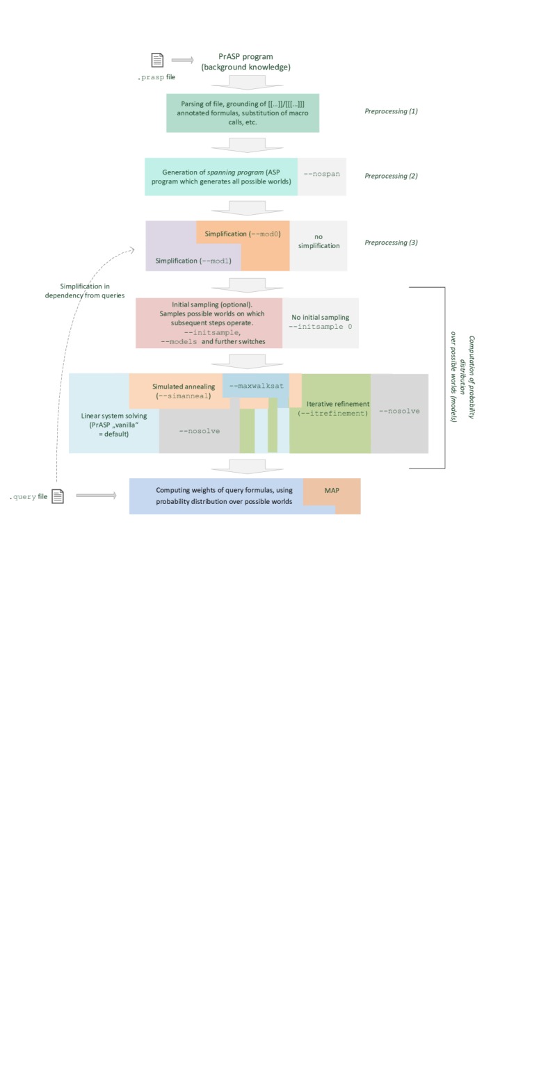
6.3 Command-line arguments
PrASP 0.9.4 is configured mainly using command-line options. Most of the switches and other arguments listed below are not required for simple use cases. However, it is suggested that you make yourself familiar at least with the inference pipeline (Fig. 3) and optimization command-line switches ( -o1, -o1asp, -o2, etc). Basic knowledge about alternative approximate solving approaches --itrefinement and --simanneal is also useful. This is because
in “vanilla mode” (the default), settings are very conservative. More concretely, using default settings, PrASP allows for maximum expressiveness in knowledge and query files but performs larger-scale tasks rather slowly. Therefore large inference or learning tasks require the use of optimization switches.
Please observe that inference-related command-line options also affect learning, since learning relies on iterated inference.
--help
for a short version of this subsection.
--verbose
shows additional information about inference and learning tasks. This information might be useful for the optimization of input files. Further information- and debugging-related switches are --check, --pwdistr, --pwsamples, --showentropy, --debug, --showindeps, --showexpansion and --showspan, which are all described further below.
--bgk file or -b file
is used to specify background knowledge (that is, a PrASP program). If --bgk and -b are omitted but a file name is provided (which is not bound by any other file name accepting command-line argument), the background knowledge file is identified based on its file name extension .prasp. Exactly one background knowledge file needs to be specified per PrASP call.
--query file_1 ... file_n or -q file_1 ... file_n
to approximate the probabilities of given query formulas within each of these files (probabilistic inference). If --query and -q are omitted but a file name is provided, the query file is identified based on its file name extension .query
Additionally, a background knowledge file is required (see --bgk).
It is possible to specify multiple --query’s per command-line, each with multiple file names as arguments. All query files in the command-line share the same background knowledge. However, for each --query occurrence (and also for each query file which is not bound by any explicit --query argument but identified by its name ending), the background knowledge is processed anew. This way, PrASP can consider different optimization strategies for different sets of query files.
--learn file or -l file
to learn weights of given hypothesis formulas within file file. If --learn and -l are omitted but a file name is provided (which is not bound by any other file name accepting command-line argument), the hypothesis file is identified based on its file name extension .hypoth. Maximally one hypothesis file can be specified with each PrASP call. If --learn or -l is specified, also --examples or -e needs to be specified.
Additionally, a background knowledge file is required (see --bgk).
--examples file or -e file
to specify learning examples (together with --learn or -l). If --examples and -e are omitted but a file name is provided (which is not bound by any other file name accepting command-line argument), the learning examples file is identified based on its file name extension .examples. Maximally one examples file can be specified with each PrASP call.
--pwsamples n
prints n sampled possible worlds (uniformly sampled with replacement).
Notice that --pwsamples n has no influence on inference or learning results, it is a purely informative task with no connection to initial sampling or --models.
--pwdistr n
prints the probability distribution over possible worlds and its entropy as obtained using initial sampling (see --initsample). If additionally --ndistrs n is specified and the default inference approach is being used (linear system solving), n distributions and their entropies are printed.
If n is specified, the number of printed worlds is limited to n. Since the results are ranked, --pwdistr can be used for MAP inference if the specified sampling or inference approach produces a probability distribution over possible worlds (or the entire set of possible worlds are top-ranked in terms of their probabilities, e.g., --maxwalksat).
--showentropy
prints the entropy of the distribution over possible worlds. In case --mod1 was used, multiple entropies are printed. No entropies are printed if interval results have been requested using --intervalresults.
The following optimization switches provide shortcuts for frequently combined command-line arguments with an influence on inference performance and accuracy. A switch with a higher number after the “o” is not “more optimizing” but just different from the other -o switches:
-o1
is a shortcut for --noindepconstrs--noautoindeps --itrefinement
-o1asp
is a shortcut for -o1 --folconv none
-o2
is a shortcut for --noindepconstrs --noautoindeps --initsample 4 --itrefinement
-o2asp
is a shortcut for -o2 --folconv none
If your input files are in pure ASP syntax, this switch should be used instead of -o2
-o3
is a shortcut for
-o3asp
is a shortcut for
-o3
--folconv none
If your input files are in pure ASP syntax, this switch should be used instead of -o3
-o4
is a shortcut for
--mod1
--noautoindeps
--noindepconstrs
--ignoreentropy
-o4asp
is a shortcut for -o4 --folconv none
If your input files are in pure ASP syntax, this switch should be used instead of -o4
--initsample m
specifies the method used for initial sampling, that is, the way PrASP generates a list of random models (possible worlds) of the spanning program used by the subsequent solving or annealing step. These initial models are passed on to the next step in the inference pipeline (e.g., they might serve as the initial distribution for simulated annealing or they are used in the linear system’s equations/inequalities). The chosen initial sampling approach and the number of initial samples (set with --models) strongly influence inference and learning speed and accuracy (in the ideal case, all models would be computed, but this is often computationally intractable).
Initial sampling either produces a set or a multiset (where the element frequencies are interpreted as a possibly non-uniform probability
distribution over possible worlds). Whether the additional information carried by the multiset (vs. a mere set) is used by the following algorithm in the inference pipeline depends on the respective next algorithm and its parameters (e.g., simulated annealing can use the result of initial sampling as a multiset, whereas the default inference approach (linear system solving) discards information about model frequencies).
Algorithms used for initial sampling are presented in Sect. 5.
If argument m or --initsample are omitted, PrASP heuristically chooses an initial sampling approach based on the information it gathered from the command-line and the background knowledge. Use --verbose to see the selected approach (which is not guaranteed to be the optimal one!).
The indicative number n of sampled models is specified by --models. If --models is omitted, a heuristically determined number of models are generated.
It is recommended to compare the sets or possible worlds and their entropies achieved with different approaches (in combination with different settings for --unisampleand other sampling-related parameters) in order to identify the optimal approach for the respective use case. See --pwdistr. Also, switch --check might be useful in this regard.
m = 0: empty set,
m = 1: n random models sampled with replacement from a near-uniform distribution. The concrete sampling approach can optionally be specified using --unisample, otherwise the approach is chosen by PrASP (use --verbose to see which one).
m = 2: any n models (random or non-random). In practice, this simply gives the first n answer sets in the stream of answer sets computed by the ASP solver. If (i.e., --models 0), all models of the spanning program will be generated (intractable unless the system is small).
m 3: n random models sampled from a distribution of models such that the frequencies of models of uncertain formulas correspond approximately to the given weights of these models if certain assumptions are met (e.g., mutual independence). So in contrast to m = 2 the formula weights are not ignored here.
The model frequencies are represented by means of the number of occurrences of the respective model in the initial sampling result list. Whether any duplicates in the resulting sample will be retained or discarded depends on the next inference stage.
Remark: most sampling approaches work significantly faster if Clingo 4 is used as ASP solver (“remote sampling”) (see Sect. 2). With Clingo 4, remote sampling is active by default where the selected sampling approach can use it. See --noremotesampling for a discussion and requirements.
Note that even weighted sampling approaches need to sample from a uniform or near-uniform distribution at some point of the sampling algorithm, that is, even with approach 3, sampling is influences by the approach specified with --unisample. The selected sampling method massively influences inference and learning performance and quality.
Methods m 3 in detail:
m = 3: a distribution is generated using random sampling with replacement such that the frequencies of sampled models fully reflect the products of the probabilities of the mutually independent weighted formulas which hold in these models. To make this
tracktable, the number of considered combinations of independent formulas might has to be limited using --limitindepcombs.
m = 4: all models are randomly sampled (stratified weighted flip-sampling, with replacement) as if weighted formulas were mutually independent (regardless of actual or declared independence). See Algorithm 3 for details.
If this independence assumption holds and the target number of samples is not too large, queries can be solved quite efficiently with m = 4 and --nosolve. Otherwise, using this option may have little benefit, or you might get no result at all (if the initial sampling process generates a lot of inconsistent sample programs). Note that the aforementioned independence assumption
does not necessarily mean that with the resulting approximate distribution holds for any actually independent events and , as this also depends from the size of the set of samples (specified with --models). The same is true for entropy: if approach 1 is used, the entropy of the resulting distribution depends on the number of samples even if in reality all events are actually mutually independent. Caveat: with --models 0, PrASP computes the set of all models of the spanning program (without replacement), which would not be useful in combination with --initsample 4.
m = 5: models are randomly sampled (stratified weighted flip-sampling with consideration of declared/discovered independence, with replacement).
This approach is similar to approach 4 above, but uses declared or discovered event (formula) independence instead of making an assumption about universal independence. See Algo. 3 for a detailed description of this approach.
Remark: flip-sampling can cause Clingo messages of the form “warning: x is never defined”. If the respective message doesn’t turn up without sampling activated then you can ignore it.
--models n
specifies the target number of initial models (possible worlds) computed during initial sampling using the approach specified using --initsample. This number and the sampling approach strongly influence inference and learning accuracy and duration.
--models is typically used together with approximate inference approaches whereas limiting the number of models in order to speed up the default inference approach is usually not a good idea (results might be highly inaccurate). It is even possible that a lower number of models increases overall inference duration, if the smaller number of models makes the solving algorithm require more time to converge to a solution for the linear system.
n is just a target - depending on the chosen sampling approach, n cannot be guaranteed (actual number of sampled models might be lower - use --verbose to see this number).
Whether initial sampling is used or not is specified by --initsample, --models just specifies the number of models sampling should generate. Exception: if n is 0 and the sampling approach set with --initsample is not 0, all models will be computed without sampling.
If --models is omitted, the target number of sampled models is heuristically determined.
In case the sampling approach specified by --initsample is 3 or 4, the default number of samples is
either as for approaches 1 and 5 (with --maxentropy) or 20 (otherwise).
The reason for the small default target number for approaches 3 and 4 without --maxentropy is that these methods
are often able to compute valid initial distributions even for a very small number of possible worlds. Increasing this number is then only required if the distribution entropy should be increased or if there are additional constraints to be observed by later inference steps (such as independence constraints). In the latter case, a following simulated annealing step in the inference pipeline automatically enhances the initial list of sampled models, provided --simanneal is also specified.
The number of actually computed samples and the estimated total number of spanning program models are printed if --verbose is provided.
Also see --unisample, --xorconf, --flipsampconf and --sirndconf.
--simanneal energy minTemp tempDecr samplingMethod initTemp samplesPerStep targetAll
uses simulated annealing as approximative inference method. It uses the models generated by initial sampling (see --initsample) as a starting point. The initial samples are treated as a multiset where the normalized count of a certain model within the multiset is interpreted as the initial approximation of the probability of that model (which is then refined by the simulated annealing algorithm). A formal description can be found in Sect. 5.3.
Because simulated annealing in PrASP relies heavily on sampling, it should be used with Clingo 4 (see Sect. 2 - however, it works with Clingo 3 too).
All arguments of --simanneal are optional.
Defaults: energy=0.05, minTemp=1e-150, tempDecr=0.95,
samplingMethod=0, initTemp=5, samplesPerStep=1, targetAll=true
Example: --simanneal 0.001 1e-150 0.95 1 5 1 false
energy () is the acceptable inaccuracy. Lower values mean more accurate results.
More precisely, this parameter specifies the maximum acceptable euclidean distance between the vector of given formula weights and the vector of weights according to the current solution candidate.
minTemp is the temperature at which the algorithm stops even if the desired accuracy has not been reached yet.
tempDecr is the factor by which the current temperature is multiplied in each step.
samplingMethod specifies the approach simulated annealing generates new samples until it found a distribution which approximates the given constraints well enough. This should not to be confused with the approach used to compute initial models (--initisample) (the set of random models simulated annealing uses as a starting point).
If samplingMethod is 0 (default), at each simulated annealing step, models are sampled from a near-uniform distribution. Use --unisample to specify the concrete approach used here.
If samplingMethod is 1, simulated annealing samples are at each step obtained using a sampling approach which takes into account declared or discovered formula independence assumptions.
samplingMethod 2 works like method 1, but makes the assumption that all weighted formulas are mutually independent, regardless of meta-statements. If this is not actually the case, this
sampling approach is very slow.
Methods with samplingMethod 3 are those one can specify with --initsample (with the difference of course that they are used for simulated annealing here, and that at each simulated annealing step only samplesPerStep random models are computed).
initTemp is the initial temperature, and samplesPerStep denotes the number of samples computed per step.
If targetAll is false, only formulas with a weight are targeted when minimizing the energy, whereas otherwise all formulas are targeted (default: false). “Targeted” means here that in the calculation of the energy, the frequency of the respective formula in the current best set of sampled models is included.
--simanneal is typically used together with --initsample, --nosolve
and --noindepconstrs. If one of these is omitted, accuracy is increased but processing time (massively) increased. PrASP shows a warning in such cases. Also consider combining --simanneal with further switches such as --mod1. The sampling step performed by simulated annealing can be further configured using --xorconf, --flipsampconf and --sirndconf.
Important: --simanneal works best if all formulas (including query formulas) are so-called
“simple formulas”, see 3.13.8. If this is not possible and inference is too slow, consider specifying an alternative model checking algorithm using --ascheckmode. Also, --simanneal profits from mutually independent formulas.
If --maxentropy is specified, simulated annealing takes the entropy (3.5) into account when computing the current energy, providing a heuristic approach to the principle of maximum entropy. However, in contrast to some other inference approaches in PrASP (like --itrefinement) simulated annealing can generally not guarantee a maximum entropy solution. Also, --maxentropy influences the initial set of models (see --initsample and --models).
--maxentropy is incorporated into the “energy” using (where is the euclidean distance between current and target weights, as described above). However, even with --maxentropy, parameter energy refers only to ,
whereas the acceptable entropy is specified using a parameter of command-line option --maxentropy.
For more information about --simanneal, please refer to Sect. 1 and Sect. 3.13.5.
--nospan
With this switch, no spanning program is being created. Useful, e.g., in connection with --maxwalksat.
--maxwalksat costtarget maxit maxtries p repl
(experimental) uses the MaxWalkSAT (weighted maxsat) algorithm [26, 18], a weight-aware variant of the WalkSAT local search satisfiability solver, to compute a number of possible worlds with larger probabilities than the rest of the possible worlds (for MAP/MPE-style inference). In contrast to normal PrASP terminology, “possible worlds” here means any satisfying truth assignments for the conjunction of the formulas in background knowledge, not answer sets of the spanning program.
All formulas (annotated or not) need to be “simple formulas” in the sense of Section 3.13.8 (you can still use non-ground or even FOL formulas with quantifiers too, but you need to make sure they are “simple” before the MaxWalkSAT phase during inference is reached, by annotating them appropriately, i.e., with [[ or [[[ weights).
costtarget specifies the acceptable cost (sum of weights of formulas not satisfied in the current candidate model at which the algorithm stops; default: 1 - you might need to provide a different value here), maxit specifies the maximum number of local search iterations per trial (default: 100000), maxtries is the maximum number of trials (default: 10000), p is the probability of taking random steps (default: 0.3), and repl (true or false) specifies whether discovered models are generated with or without replacement (default: true, only relevant if you want to use MaxWalkSAT to produce more than one possible world).
MaxWalkSAT262626and also the other Markov Logic-like inference approach built into PrASP , see --mln and Section 3.10 fits well into the overall PrASP inference pipeline (Sect. 6.2), but in one respect it is exotic among the PrASP inference approaches - it treats formulas as propositional formulas and solves them in the sense of SAT solving (which is closely related to but not identical with ASP solving). It does not follow stable model semantics and it does not use an ASP solver, provided it is used with --nospan. An external ASP grounder is required if any of the formulas in background knowledge or query file are non-ground (but in that case they must be annotated with double- or triple-square brackets, in order to produce ground formulas before the MaxWalkSAT stage!) and cannot be grounded internally. As a side note, observe that ASP grounding using an external grounded is already “lazy” in the sense that it omits ground instances about which it knows that they have no influence on models.
With --maxwalksat, PrASP can be used without ASP solver, provided the query formulas are also “simple formulas”. To enable this, specify additional switches --nospan --assumegroundersolver 0
. If your background knowledge is ground already, you also don’t need an ASP grounder.
MaxWalkSAT can be combined with --initsample. There are two major ways to do this:
-
•
specify
--initsample 0 --models n --pwsamples --nosolve --nospan--noindepconstrs --ignoredeclindeps --noautoindepswheren. In that case, no initial samples are generated and MaxWalkSAT generatesnpossible worlds (approximately the ones with the highest probability) all by itself. Ifn= 1, this emulates Markov Logic’s MAP inference.
To project the model to certain literals, provide these literals as individual query formulas - where the probability is 1, the literal is true in the model (ifn). Alternatively, use --pwsamples to see the entire generated set of possible worlds. -
•
specify some --initsample approach other than 0 (empty set) and, using --models, a number of models . In that case, the initial models are used as seeds for MaxWalkSAT: for each MaxWalkSAT try, a randomly picked initial model is used as the initial “guess” (which would be a random truth assignment instead if there are no initial models). This way, MaxWalkSAT replaces the sampled initial models with new models.
Although probably not advisable, it is possible to use the output of MaxWalkSAT as input (subset of the set of all possible worlds) for subsequent inference stages, such as iterative refinement (--itrefinement).
It is also possible to let PrASP perform preceding steps besides --initsample, such as --mod1 for program simplification.
In some cases (see above) MaxWalkSAT is used together with --nospan, as MaxWalkSAT doesn’t require or use a spanning program.
Caveats/issues:
-
•
Under PrASP semantics, formula weights denote point probabilities or probability intervals. In order to emulate weights of “hard constraints” (using MLN terminology), our MaxWalkSAT variant counts formulas annotated with weight 1 as well as unannotated formulas as if they had weight 1000 (instead of the infinite weights of hard rules in MLN).
-
•
There is currently no MaxWalkSAT support for conditional probabilities or independence constraints in background knowledge, however, conditional probabilities in queries are fine.
-
•
MaxWalkSAT maximizes the sum of given formula weights. It doesn’t take into consideration at weight maximization any implied weights of formulas which don’t appear explicitly in background knowledge. Switch --addnegf might be helpful in this regard.
-
•
MaxWalkSAT is efficient only for MAP/MPE-style inference, i.e., to compute a single (or a very small) number of possible worlds with maximum (or close to maximum) weight.
-
•
All of the currently supported schemes for translating FOL formulas into ASP syntax (such as F2LP) assume stable model semantics, that is, if used with a non-stable model-based approach to model generation (such as MaxWalkSAT), unexpected query results are to be expected.
-
•
For Markov Logic Network-style inference, see
--mln.
The algorithm of PrASP’s MaxWalkSAT variant is presented in Sect. 5.7.
Remark: there is currently no LazySAT in PrASP , as LazySAT would be incompatible with PrASP ’s approach to grounding. However, notice that if PrASP employs the external grounder for grounding, this grounder typically applies simplifications.
--itrefinement epsilon n retainCounts§
uses the inference approach introduced in [16] (called iterative refinement in PrASP terminology) to compute a possible worlds probability distribution with maximum entropy (where the entropy is bound by the initial set of possible worlds provided as input for this approach. With smaller sets, the entropy typically also decreases).
Iterative refinement is often a good first choice if the system is just too large for the default “vanilla” inference approach. However, it requires a “good” set of initial samples - if the set of sampled models is too small or not random enough, you will get no or inaccurate results. Use of --check is advised.
If --models isn’t provided, PrASP samples a heuristically determined number of random models (which is not guaranteed to be optimal).
Iteration stops if the maximum number of iterations n (default: 1000) is reached or if the euclidean distance between the probability distribution computed in the current step and the distribution obtained in the previous step falls below threshold epsilon (default: 0.02).
To make this approach tractable for complex background knowledge, --itrefinement can be combined with --models and --initsample in order to reduce the number of models on which this approach operates (but a smaller number of sampled models also decreases entropy). Actually, if these arguments are not provided, PrASP heuristically selects a sampling approach and a number of samples. If you want to enforce that iterative refinement should use the full set of models of the spanning program (for more accurate results, possible with small systems), provide arguments --initsample 2 --models 0
Iterative refinement starts by default with the uniform distribution over all models generated by the initial sampling step (discarding any duplicates if the initial samples are a multiset). Alternatively (if retainCounts is true), it also uses the frequencies of models generated by initial sampling as a starting point. The initial samples are then treated as a multiset where the normalized count of a certain model within the multiset is interpreted as the initial approximation of the probability of that model. However, there are no entropy guarantees anymore in that case.
The algorithm is presented in Section 5.6.
Providing switch --maxentropy has no direct influence on the --itrefinement algorithm (which intrinsically maximizes entropy, given a certain number of samples). However, --maxentropy might influence the number of initial samples computed with --initsample and might thus indirectly also influence the entropy of the solution distribution.
If specified, iterative refinement replaces the linear system solving approach in the inference pipeline, so --nosolve should normally not be specified together with --itrefinement (it is possible to use --itrefinement with --nosolve, but it is unclear yet if this combination provides any benefits).
A major benefit of this approach is that the entropy of the computed solution depends on the
number of initial samples, i.e., you can increase the entropy by providing a larger number
of sampled models or by changing the initial sampling approach. But of course, generating a larger, uniformly distributed number of models increases computation time too. Maximum entropy can be achieved by using all models of the spanning program using initial sampling approach 2 (which obtains all answer sets of the spanning program), but this is of course intractable for all but the most simple background knowledge programs.
Notice that convergence of iterative refinement (in the way it is used in PrASP ) does not guarantee that the query results reflect your constraints (formula weights, rules, etc). If the list of models obtained using initial sampling is too small or biased, query results are wrong regardless of epsilon.
It is thus recommended to use --check together with --itrefinement.
--itrefinement can theoretically be combined with --simanneal as a sampling approach (in that case, --nosolve is also omitted although --simanneal is given), but this combination has no known benefits.
--itrefinement currently doesn’t work with --intervalresults (but intervals can be specified in background knowledge).
Independence declarations and discovered independence are not enforced by the iterative refinement algorithm (but the fact that the algorithm maximizes entropy compensates for this to some degree). However, independence declarations or discovered independence might still be considered during initial sampling, depending on the initial sampling approach (see --initsample).
--ascheckmode m
specifies the approach to be used for answer set checking.
PrASP performs Answer Set Checking (ASC, a form of model checking) at various points. ASC determines whether
holds for a model and some ASP program . When PrASP checks a model for a single formula in the background knowledge, where is the spanning program of . We sometimes write instead of .
When PrASP checks a model for a single query formula , where is the program consisting of all unannotated formulas in the respective query file.
This switch specifies the approach being used if is not a so-called “simple formula” 3.13.8 in the context of the spanning program.
With m = -1 (default), the approach is automatically chosen using a heuristics depending from the number of computed models of the spanning programming.
m = 0: iff satisfiable for (checks consistency with model).
m = 1: iff where is the set of all answer sets of .
m = 2: like m = 1, but only a uniformly sampled subset of answer sets of is used where is the number of models specified using --models (generally unsound).
For small systems, m = 1 is typically fastest but intractable for larger systems for which m = 0 works better.
--mod0
(experimental!) simplifies certain ASP ground rules whose bodies consist entirely of literals which are declared probabilistically mutually unconditionally independent. --mod0 requires a special design of the background knowledge to be useful in practice, otherwise the time required for the extra analysis caused by --mod0 exceeds any performance gain. Requires that weighted formulas with single bracket weights (i.e., of form [w] f) are ground. Typically used in connection with --mod1. See 3.13.7 for details.
Note that --mod0 currently considers mutual independence only. Furthermore, in contrast to default setting, --mod0 requires formulas to be fully parsed locally (i.e., by PrASP itself, not just by the ASP grounder), which currently induces limitations wrt. Gringo4 formula syntax supported with --mod0.
--mod1
(experimental!) simplifies background knowledge with the aim to remove all parts which have no influence on the result of queries. This filtering step might make a normally intractable task solvable (even with precise inference approaches). The aim of this feature is remotely similar to the identification of the minimal Markov network required for answering a query in Markov Logic [18].
See 3.13.7 for details. Requires that weighted formulas with single bracket weights (i.e., of form [w] f) are ground.
--mod1 only has a positive effect if the gain achieved by the simplification is bigger than its cost (time required for analyzing and simplifying the spanning program).
--mod1 does not comprise --mod0, both switches are independent from each other and can be used together or alone.
Note that in contrast to default setting, --mod1 requires formulas to be fully parsed locally (i.e., by PrASP itself, not just by the ASP grounder), which currently induces limitations wrt. Gringo4 syntax supported with --mod1.
--noautoindeps
disables the automated identification of mutually independent atoms. Manually declared independent formulas are not affected by this switch. Use this switch in case you know which formulas are independent and you have declared these yourself independent in the background knowledge (using meta-statements such as #indep, etc), or in case the automated identification includes atoms you wish to treat as non-independent (use --showindeps to see which atoms PrASP considers to be independent),
or in order to increase processing speed in case the constraints introduced in order to enforce
independence among these atoms slow down inference (but see --mod0). For more details about independence handling see #indep...#endIndep (meta-statement #indep) and 3.13.
--ignoredeclindeps
ignores all declared independence (meta-statements such as #indep). Observe that even with this switch, certain sampling methods might make implicit independence assumptions (e.g., --initsample 4).
Also consider --noindepconstrs and --noautoindeps.
--noindepconstrs
specifies that PrASP should not generate probability constraints for mutually or pairwise independent atoms (automatically discovered as well as manually declared ones). If this switch is not present, and event independence has been declared or discovered, inference algorithms observe constraints which enforce that for any two independent events , . The algorithms affected by this are currently linear system solving, linear programming and simulated annealing. Any other use of formula independence (e.g., with --mod0) is not affected by this switch.
It is important to not confuse independence enforcement with the independence assumption made by some (but not all) algorithms in PrASP ; --noindepconstrs only disables the enforcement of independence relations. For further details about independence handling see #indep...#endIndep (meta-statement #indep) and 3.13.
--noindepconstrs does not imply/is not implied by --noautoindeps or --ignoredeclindeps.
--limitindepcombs n
limits computation of combinations of mutually independent formulas to length n. Leads to wrong results for if results depend on the assumption that are independent for any .
--check
makes PrASP print information useful for estimating the accuracy of inference results. Concretely, it shows the differences between the given weights of formulas in background knowledge and the inferred probabilities for these formulas. Constraints imposed on probabilities due to independence declarations and initial sample entropy are not checked (but see --showentropy and --pwdistr).
A different kind of check is provided using --checkconsistency
--checkconsistency
lets PrASP check the logical and probabilistic consistency of the specified background knowledge. Note that this slows down inference. A different kind of check is provided using --check
--showindeps
shows the set of formulas which PrASP considers to be logically independent of each other.
--cacheinfsetup
enables a cache for inference setups. Significant speed gains if inference and learning tasks comprise repetition (in particular with streams which contain repetitions of the same floating windows), but might make inference and learning slower in other cases.
--unisample m
specifies the approach used for sampling from a (near-)uniform distribution of models. Choosing a sampling approach which is appropriate for the problem at hand can make a dramatic difference wrt. inference and learning speed.
--unisample affects almost all places where uniform sampling is performed, including where uniform sampling is a helper task for weighted sampling. This affects most of the initial sampling approaches but also sampling which is part of inference approaches like simulated annealing. An exception are those places where flip-sampling needs itself to call a uniform-sampling approach (see --flipsampconf).
m = -1: auto (let PrASP decide, use --verbose to see selected approach), 0: random models from full set of models (high quality but can be very slow), 1: (uniform) flip-sampling (see Section 5.4; where applicable, which is where the sampled models are answer sets of the spanning program), 2: XOR-sampling (Algorithm 4), 3: ASP solver-internal randomization (if applicable; see --sirndconf for details), 4: like 1, but only formulas which are known to be independent are flipped.
These methods can be further configured using --xorconf, --flipsampconf and --sirndconf.
If there are dependencies between the events in your program, try XOR-sampling first. If you know that all events are mutually independent, try flip-sampling first. Method 3 is typically fastest, but of low sampling quality (large bias).
Uniform flip-sampling (which can be seen as a meta-sampling approach) itself needs to obtain uniformly sampled models from a randomly modified variant of the spanning program, and it does so using some other approach to sampling, namely the approach specified using --flipsampconf (or a default method). Again, this choice influences sampling quality.
Observe that --unisample does not “activate” (near-)uniform sampling, it merely specifies the approach used for (near-)uniform sampling.
--xorconf q1 q2
specifies the quality of near-uniform sampling using XOR streamlining constrains [7]. This sampling method is underlying most sampling tasks in PrASP , including some of the initial sampling approaches and simulated annealing.
q1 is the number of models requested with each ASP solver call (default: 100). The larger q1, the better the sampling quality (uniformity) and the slower the computation of samples. With q1 = 0, the samples requested will
be chosen randomly from all models computed using XOR constraints (i.e., the random subset of all models of the respective XOR-constrained ASP program. Best quality, slowest).
q2 is the number of XOR constraints generated per sampling step (if q2 is omitted, a heuristics is being used). See Algo. 4 for details.
Note that this command-line argument does not “activate” XOR-sampling, it just configures it.
Sampling using XOR streamlining constraints is formally described as Algorithm 4.
--sirndconf o
configures sampling without use of XOR streamlining constraints, using ASP solver-internal randomization instead. This is faster but often obtains significantly lower degree of uniformity compared with XOR-sampling, i.e., less accurate results or slower convergence rate if combined with sampling-based inference such as simulated annealing.
--sirndconf affects all sampling tasks in PrASP where solver-internal randomization can be used, including initial sampling with --initsample.
is an optional multiplier which influences the size of the set of models from which samples are chosen randomly. The size of each set is where
is the requested number of samples. The higher , the better is the sample quality, except for the following: With , and if the respective sampling task is without replacement, samples are selected randomly from a uniform random distribution of all models (very slow for large systems). Default is 100.
Note that this command-line argument does not “activate” solver-internal randomization, it just provides an opportunity to configure it when solver-internal randomization is selected with, e.g., --initsample or --flipsampconf.
Alternative ASP solver parameters for randomization can be specified using --groundersolver.
--flipsampconf r
configures flip-sampling (both uniform and weighted). If r is 0 (default), each time the flip-sampling algorithm requests a model sampled from the uniform distribution, it uses the first model generated by the solver with solver-internal randomization activated. This is much faster but less “uniform” than the other available approaches here, where the uniformly-sampled model is either obtained randomly from all models of the spanning program with flipped formulas (r = 1) or using XOR-sampling (r = 2). If r is 0, solver-internal randomization quality can be further configured using --sirndconf or --xorconf. These three approaches can also be used directly (without flip-sampling).
Note that --flipsampconf does not “activate” flip-sampling, it just allows to specify its parameters.
Flip-sampling is formally described in Section 5.4.
--noremotesampling
enforces that always the older (pre v0.8) approach to invoke the ASP solver for sampling is being used even where the more recent Clingo4-based remote sampling would be possible.
Remote sampling means that Clingo 4 is used with Lua-script clingo4Sampling.lp for certain sampling approaches. Remote sampling is typically much faster than the older approach. Unless --noremotesampling is specified, PrASP automatically chooses in which situations clingo4Sampling.lp is used. At this, PrASP maintains a standing connection to the external ASP solver, with communication with PrASP via TCP/IP. Sampling via (stratified or unstratified) weighted or unweighted flip-sampling algorithms is performed on client side, which makes sampling massively faster. Furthermore, weakly uniform sampling using solver-internal randomization is supported.
clingo4Sampling.lp is a Lua-script, so if you like you can provide your own sampling approach “on-the-fly” without having to change PrASP itself.
The algorithm for remote flip-sampling currently implemented by the Lua script is, for technical reasons, somewhat different from the PrASP -internal one, see Algo. 3.
There are currently a few restrictions in connection with remote sampling:
- flip-sampling using clingo4Sampling.lp requires that only atoms have weights attached (or rules where PrASP is able to simplify the body away during grounding if annotated with [[...]]/[[[...]]]). This is not a serious restriction for most use cases, since Annotated Disjunctions can still be used (they are de-sugared into unweighted rules and weighted atoms).
- The combined grounder-solver needs to be Clingo 4 (version 4.5.3 or higher). Other ASP grounders/solvers are not yet supported with remote sampling.
--nosolve
omits possible world weight computation by linear equation system solving or linear programming (optimization) when doing inference. Query probabilities are determined by direct counting of models. --nosolve requires that at least one of the following prerequisites holds in order to obtain approximately correct results:
-
•
An initial sampling approach which immediately provides a valid possible worlds distribution. This is doable if all weighted formulas are mutually independent. See --initsample for details.
-
•
Switch --simanneal is provided
-
•
Switch --weights2cc is given together with background knowledge where weighted formulas represent mutually independent events.
-
•
Unweighted background knowledge which is manually designed such that the models (obtained using initial sampling) of its spanning program represent the desired probability distribution (not always possible). Weights are entirely ignored here.
--mlns
(experimental!) emulates Markov Logic Network [18] semantics - to some degree in the style of [20], i.e. combined with stable model semantics.
Weighted rules where the weight is below 1 are interpreted as soft rules whereas other rules become hard rules in the MLN sense (i.e., weight 1 corresponds to MLN’s infinite weight). Weights in background knowledge do not denote probabilities anymore, whereas weights resulting from queries are still probabilities.
This switch needs to be combined with –--noindepconstrs. Also, it doesn’t support conditional probabilities in background knowledge (they are simply ignored). However, conditional probabilities can still be used in query files.
See Sect. 3.9 for an example for how to use this switch.
Also see --maxwalksat.
--intervalresults
makes PrASP return for each query formula a range of probabilities for this query (lower and upper bounds), i.e., query results become probability intervals.
If no other inference approach is specified, this makes PrASP use a simplex solver (linear programming) to compute a probability interval for each query formula. The solver can be configured using --linoptimconf.
Note: --intervalresults is not required for the specification of probability intervalsin background knowledge.
See 3.5 for further details about probability intervals.
--linoptimconf epsilon fpcompULP cutoff maxit
configures the linear programming approach used by PrASP .
epsilon specifies threshold for algorithm convergence (default: 0.001). fpcompULP (deprecated) is the Units in the Last Place for floating point comparison (default: 10), cutoff (deprecated) is the cut-off value for pivot value selection in the simplex method (elements smaller than cutoff will be treated as zeros; default: 1.0E-10), and maxit is the maximum number of iterations before the algorithm gives up (default: 100000).
fpcompULP and cutoff are deprecated and their values are ignored with the current linear programming solver.
--linsolveconf approach regularizer
With the “vanilla” approach to inference, PrASP computes the probabilities of possible worlds by calculating or approximating the solution of a system of linear equations (see Sect. 1). If there are no intervals in background knowledge and also no queries with intervals, the following approaches are currently provided.
Note that while some of the approaches below (in particular native and CUDA solvers and iterative approaches to LS) are very fast, the true bottleneck with the “vanilla” approach to inference is not the system solver or LS method but the time required to compute a very large number of models (possible worlds).
PrASP uses either (NN)LS (with SMT as fall-back) or linear programming. (NN)LS is configured using this switch whereas linear programming is configured with --linoptimconf and enforced using --intervalresults.
approach is a number which specifies the concrete Linear Least Squares method. By default (-1), PrASP uses for its “vanilla” inference approach the Biconjugate Gradient Stabilized Method with regularizer 0.001 (unless the system size is below 170x170, then SVD is used by default). Exceptions if --enforceSMT or --checkconsistency or --maxentropy are specified: with --checkconsistency, Singular Value Decomposition (SVD) with one additional SVD call is enforced and with --maxentropy, we use a single SVD with a subsequent gradient descent search for entropy maximizing distributions (search is not guaranteed to succeed - consider --itrefinement as a truly entropy maximizing alternative).
regularizer (optional) is a number between 0 and 1 which specifies the regularization constant applied to increase the robustness of the solver. The larger this value, the more robust the solver becomes (more often finds a solution) and the less accurate are inference results.
- Non-Negative Linear Least Squares (NNLS)
-
(
approach= 0) using Lawson and Hanson’s method [44] (as withlsqnonnegin MATLAB) backed up with a QR-based non-constrained least-squares solver (native or on GPU, where available). While Lawson and Hanson is not the fastest approach to NNLS, it is quite robust and faster than the also robust L-BFGS-B. - Fast Non-Negative Linear Least-Square (FNNLS)
-
(
approach= 1) using the algorithm proposed in [45] (variant of Lawson and Hanson’s method). - Non-constrained Linear Least Squares (LS)
-
based on non-iterative or iterative approaches. Non-constrained LS is not a general inference approach in PrASP but if it finds a solution it does so faster than the NNLS approaches.
- Non-iterative approaches
-
provided are SVD-decomposition, QR-decomposition or Cholesky-decomposition. Cholesky is fastest but least robust. SVD is typically most accurate but slowest and QR is on the middle-ground between the others. These approaches are typically faster than NNLS, however, they don’t necessarily compute a probability distribution. If no valid solution is returned, PrASP attempts to use the invalid solution and the linear system’s kernel basis (if available) as a starting point to find valid solutions, provided the system is underdetermined.
approach= 10: QR decomposition using CUDAapproach= 11: Cholesky decomposition using CUDAapproach= 12: QR using LAPACK/BLASapproach= 13: SVD using LAPACK/BLASapproach= 14: QR using Apache Mathapproach= 15: SVD using Apache Math
For more precise results, it is advisable to use SVD (approach= 13 or 15). - Iterative approaches
-
in PrASP are the Biconjugate Gradient Stabilized method (BiCGstab) and the Generalized Minimal Residual method (GMRES). The latter is particularly useful with sparse systems. Given that rules tend to be true in all possible worlds (and they always are if they are not weighted), we can often increase sparsity by flipping the coefficients of matrix A (which denote whether the respective row formula holds in the respective possible world) and negating the row formulas (i.e., replacing their weights with 1-weight).
approach= 20: BiCGstab based on LAPACK/BLASapproach= 21: GMRES based on LAPACK/BLAS
SVD non-constrained LLS is used with subsequent search for further solutions using the system’s null space (kernel). This does not guarantee a solution but is quite fast if it finds one. Also, it allows to find a maximum entropy solution in case of an underdetermined system.
Matrix decompositions can be computed, where available, using CUDA (i.e., on the NVIDIA graphics processor) or using an external native LAPACK library. Performance of CUDA naturally depends on the speed and memory of the Nvidia GPU in your machine.
LAPACK/BLAS native linear algebra libraries need to be specified on the command line, using JVM -D parameters. If these are missing, Java implementations are used, which are naturally slower.
Various alternative libraries can be specified here (commercial as well as free ones), with different performance characteristics. To enforce the use of a particular implementation, modify prasp.sh or prasp.bat. Example:
ΨΨ
ΨΨ-Dcom.github.fommil.netlib.BLAS=com.github.fommil.netlib.NativeRefBLAS
ΨΨ-Dcom.github.fommil.netlib.LAPACK=com.github.fommil.netlib.NativeRefLAPACK
ΨΨ-Dcom.github.fommil.netlib.ARPACK=com.github.fommil.netlib.NativeRefARPACK
ΨΨ
To deactivate the use of native BLAS, LAPACK and ARPACK libraries, specify
ΨΨ-Dcom.github.fommil.netlib.BLAS=com.github.fommil.netlib.F2jBLAS
ΨΨ-Dcom.github.fommil.netlib.LAPACK=com.github.fommil.netlib.F2jLAPACK
ΨΨ-Dcom.github.fommil.netlib.ARPACK=com.github.fommil.netlib.F2jARPACK
ΨΨ
The (NN)LS approaches minimize the 2-norm , so they return a probability distribution (and thus query results) even where the linear system does not have a solution (i.e., if your background knowledge is inconsistent).
For handling of intervals, see --intervalresults and 3.5. The basic difference to the approaches listed above is that with intervals, PrASP uses linear programming as default approach. In contrast to (NN)LS, linear programming minimizes the 1-norm instead of the 2-norm of , where the latter is otherwise preferable (as it is differentiable). Alternatively, PrASP can also use the SMT solver as fallback solution to interval handling (but this is much slower).
--ndistrs n
performs inference using n probability distributions over possible worlds (n ). Default: n = 1. --ndistrs n works only with the default inference method (linear system solving).
Each query formula might then result in multiple alternative probabilities (not necessarily different from each other).
For unconditional query formulas, these probabilities are separated by “,’ ’ and listed in the order corresponding to the sequence
of probability distributions which have been used.
Consider using --intervalresults instead of --ndistrs. For details, see Sect. 3.5.
--maxentropy p nsc st r
(experimental!) activates heuristic options in inference and sampling algorithms so that the entropy of the computed probability distribution over possible worlds is increased compared to the default settings. How much the entropy can actually be increased depends on the chosen sampling and inference approaches. --maxentropy is currently effective on the default inference approach (linear system solving with point probability results) and - to a limited degree - for simulated annealing.
--maxentropy also influence the sampling of initial models, see --models and --initsample. --maxentropy has no direct influence on --itrefinement but might indirectly influence the entropy of the iterative refinement result via the number of initial models.
Note that a general limiting factor for entropy is the number of initial models set by --models (more models lead to higher entropy).
Optionally, and if linear system solving is used (PrASP “vanilla”), you can specify the desired precision p wrt. entropy of the distribution search algorithm (lower value means higher precision and longer computation time). Default precision is .
If parameter nsc is true, the algorithm doesn’t stop if the search direction changes (default: false).
If parameter st is true, Stochastic Gradient Descent is used (vs Batch Gradient Descent). Default is false.
r is a value by which the algorithm replaces encountered zeros during the computation of the derivative of the KullbackLeibler divergence during Stochastic Gradient Descent. If you encounter “sign change” errors, try a smaller value than the default of 1e-6.
These parameters are only available with linear system solving.
If inference method is simulated annealing, p has a different meaning: it specifies the maximum acceptable coefficient of variation (relative standard deviation) of the list of all entropies (of the candidate distributions computed by the simulated annealing algorithm). If the coefficient has not yet fallen below p, the search for a distribution with higher entropy continues. Default value for p is here 0.15. nsc and st are ignored.
For other inference methods, all parameters of --maxentropy are ignored (and it depends on the inference approach whether --maxentropy has any effect at all). For details, please see Sect. 3.5.
--ignoreentropy
makes PrASP ignore the entropies of candidate probability distributions over possible worlds if inference is performed using linear system solving. Can be used to obtain faster results (which might carry an unwanted information bias though) or
as an alternative to --intervalresults in connection with --ndistrs (here --ignoreentropy computes a number of biased solution whose minimum and maximum values approximate the interval of all valid solutions).
In the absence of both --maxentropy and --ignoreentropy in connection with linear system solving as inference method, PrASP computes a small number of sample distributions and chooses the one with the highest entropy. This obviously does not guarantee maximum entropy but merely aims at avoiding minimum entropy.
Note that --ignoreentropy does not mean that the resulting probability distribution has a low entropy, just that PrASP does not apply any entropy-increasing measures.
--enforceSMT
tells PrASP to always use the external SMT solver in place of the internal linear system solver.
--omitSMT
causes that the external SMT solver is only called in case the internal solver could not find at least one probability distribution. Otherwise, the SMT solver might be called even in case a distribution was already found by the internal solver, in order to generate additional possible worlds.
--weights2cc
--strongnegbelief
(experimental!) uses strong (classical) negation for modeling opposite beliefs and creation of possible worlds from uncertain knowledge. Default is use of default negation (negation as failure). Also note that due to the way F2LP operates, the strong negation of complex formulas (vs. atoms) might be identical to the default negation.
But generally, inferred probabilities of formulas and might differ from each other. If you want to ensure that they are identical, you can e.g. enforce a strong closed world assumption for some predicates by adding rules of the form -p :- not p. However, note that classical negation is essentially just a syntactic feature of literals in the input language of ASP grounders/solvers such as Gringo/Clingo.
--addnegf
generates additional constraints for negated weighted formulas. E.g., in addition to [0.3] f, formula [0.7] not f is generated (respectively weighted literal [0.7] -f with --strongnegbelief).
--spangenconf useFOL2ASP
allows to configure the spanning formula generation policy. If useFOL2ASP is true (default), spanning formulas are created from FOL forms of non-ground ASP formulas, where possible (provided a FOLASP converter is specified). Otherwise, PrASP creates them without the intermediate FOL form (experimental).
--spanqueries
(experimental!) adds spanning formulas of the form for each query formula . This implicitly creates a prior probability for each query formula (0.5 in case the formula is independent).
--dnf
(deprecated) uses the Disjunctive Normal Form (DNF) of query and weighted formulas instead of their answer sets to check their truth in possible worlds. In older versions of PrASP , use of --dnf could significantly speed up inference if weighted and query formulas are very small, but with current PrASP versions, --dnf is usually much slower than the default approach and other optimization means. Even more important: --dnf doesn’t observe stable model semantics and isn’t fully compatible with ASP syntax and semantics (e.g., no nested terms allowed).
--dnf can be used with basic FOL syntax constructs, just observe that the internal translation of FOL formulas adds computation time, of course. This switch might disappear in future versions of PrASP .
--assumegroundersolver c
forces PrASP to make an assumption (without checking) about the presence and version of the grounder/solver being used. If c = 0, it is assumed that Gringo/Clingo/Lparse is not used. If c = 1, a Gringo 3/Lparse/Clingo 3 grounder/solver is assumed, and with c = 2, Gringo/Clingo 4 is assumed. Default = -1 (no assumption, automated detection is used).
--grounder filename "arguments" "plain text arguments"
specifies the external ASP grounder (if omitted, a default external grounder binary will be used, which is currently gringo (Linux), gringo.exe (Windows) or gringo_macosx (Mac)).
"plain text arguments" are those arguments which are used when the grounder is asked for plain text grounding output (e.g., "-t" if the grounder is Gringo or Lparse).
Example: --grounder "gringo4_macosx" "" "--text"
The grounder must match the combined grounder/solver being used. E.g., if you specify Gringo 3 as grounder, you must specify Clingo 3 as combined grounder/solver (using argument --groundersolver).
Observe that PrASP does not (and cannot) check what the specified program is actually doing, so this switch should be used with care.
--groundersolver filename "arguments" "randomization arguments"
specifies the external combined ASP grounder+solver. If omitted, a default external grounder+solver binary will be invoked, which is currently clingo (Linux), clingo.exe (Windows) or clingo_macosx (Mac).
"arguments" is the list (enclosed in "…") of arguments passed to the program, "randomization arguments" (enclosed in "…") are
those arguments which are passed to the program if the program should randomize the returned set of models (solver-internal randomization, see --sirndconf).
In "arguments", any occurrence of %NUM is replaced with the number of requested models, or 0 if all models are requested. Any occurrence of %NZNUM is replaced with the number of requested models, or 2147483647 if all models are requested.
In "randomization arguments", any occurrence of %SEED is replaced with a random number.
Default arguments (subject to change in later versions):
With Clingo 4: -n%NUM --verbose=1 --project --save-p=70 --config=jumpy
With Clingo 3: --shift -n%NUM --verbose=1 --project --save-p=70
Default randomization arguments (subject to change in later versions):
With Clingo 4: --project --sign-def=3 --rand-freq=0.9 --restart-on-model --seed %SEED -n%NUM --verbose=1
With Clingo 3: --shift --project --rand-freq=0.9 --restart-on-model --seed %SEED -n%NUM --verbose=1
Example:
--groundersolver "clingo4_macosx"
"-n%NUM --verbose=1 --project --save-p=70 --config=jumpy"
"--project --sign-def=3 --rand-freq=0.9 --restart-on-model --seed %SEED -n%NUM --verbose=1"
The specified grounder must of course be compatible with the combined grounder/solver being used. E.g., if you specify Gringo 3 as grounder (using argument --grounder), you must specify Clingo 3 as combined grounder/solver.
Observe that PrASP does not (and cannot) check what the specified program is actually doing, so this switch should be used with care.
--groundingconf groundPreContext allowInternalGrounding sortDomains revertDomains omitBgkInQueryContext genSpanInContext "parameters"
influences how formulas are being grounded, in particular those annotated with [[...]] or [[[...]]].
None of its arguments are optional, you need to specify all seven arguments here.
Default values correspond to --groundingconf 1 true true -1 false false ""
If groundPreContext is 1 (default) then PrASP calls the external grounder in order to obtain the set of ground domain predicate instances (which is then used to internally determine the domains of ASP variables) from the grounding precontext (basically all unannotated formulas). If it is 0, only ground facts which are explicitly provided are considered as domain predicate instances and variable instantiation during internal grounding. This severely restricts the grounding process but avoids an external grounder call. Even with groundContext=0, PrASP is still able to use simple intervals such as p(1..3,5..9) and sequences such as p(a;b;c) to obtain ground domain predicates, however, to obtain the grounding precontext (Sect. 4.4) from more complex such formulas (e.g., with variables as interval boundaries), it needs an external grounder (this restriction applies to the step of grounding the grounding precontext in order to obtain ground domain predicate facts).
If allowInternalGrounding is true (default), PrASP grounds basic [[..]]- or [[[..]]]-annotated ASP formulas itself without the help of an external grounder. This is not necessarily faster (there is no expensive call of an external grounder tool, but on the other hand the grounding method is likely slower than that of the external grounder), but allows PrASP to fix the order of generated formula ground instances (which is otherwise undetermined).
Note that internal grounding still makes use of the external grounder (if present), namely in order to expand domain predicates in the unannotated part of the program.
If sortDomains is true (default), PrASP sorts the resulting ground instances lexicographically and token-wise (where the tokens are the words and numbers in a formula).
With revertDomains = 1, the order of the sequences of instances of domain predicates is reversed. With revertDomains = 0, the original sequence is kept, and with revertDomains = -1 (default), reversion is determined automatically. Note that there is no way to ensure that revertDomains determines the order of generated formula ground instances if an external grounder is being used.
If omitBgkInQueryContext = true (default: false), the background knowledge’s grounding precontext is not added to the queries’ grounding precontext. This is particularly useful if the unannotated part of the background knowledge is large and the query file contains all information needed to ground [[..]]- or [[[..]]]-annotated formulas in the query file.
If genSpanInContext is true (experimental; default: false), for each weighted formula in background knowledge, its spanning formula is added to the grounding precontext, whereas normally the grounding precontext only comprises unannotated formulas given directly in the file. genSpanInContext can help grounding [[...]] or [[[...]]] annotated formulas whose grounding depends on other weighted formulas.
parameters (enclosed in "...") is a string with extra parameters (separated by whitespace) passed to the grounder. Default is "". With Gringo 4, you could provide --keep-facts here in order to protect atoms in normal rules from being simplified away. However, even with this, the external grounder might perform certain simplifications which cannot be deactivated (e.g., of aggregates).
Another means to influence grounding is meta-statement
#dontExternalize...#endDontExternalize, see Sect. 4.7.
If you are not sure about the result produced with the various options, you can use --showexpansion to check if the resulting sequence of ground instance is what you had in mind.
--folconv convertername
specifies the optional FOLASP converter. This can be either the built-in converter FOL2ASP (specified using --folconv internal) (this converter is also used if --folconv is missing) or some external converter, such as F2LP [3] (in that case, specify --folconv f2lp (Linux), --folconv f2lp.exe (Windows) or --folconv f2lp_macosx (Mac).
Use --folconv none to deactivate FOLASP conversion (speeds up PrASP ).
Note that if --folconv none is not specified and a converter is found, PrASP might call the converter even if the background knowledge and queries are in ASP syntax.
Observe that PrASP does not (and cannot) check what the specified program is actually doing, so this switch should be used with care.
The built-in converter FOL2ASP uses almost the same algorithm [3] as F2LP, however, there are a number of technical differences:
-
•
FOL2ASP is still somewhat less mature than F2LP
-
•
FOL2ASP provides better compatibility with Gringo 4 than F2LP 1.3: Gringo3/Lparse
#domainstatements are still supported but there is also support for the new syntax![X,Y,Z,dx(X),dy(Y),dz(Z)]:(analogously for?[...]:) where predicatesdx,dy,dzspecify the domains of the variables. Equivalent to![X,Y,Z]: ... <- ..., dx(X), dy(Y), dz(Z), however, we automatically use these domains for newly introduced helper variables too. Only one binding (atom) per variable allowed. Also, use of this syntax might lead to another variable renaming (introduction of a new variable), to make sure that domain predicate bindings are unique for their respective variables (e.g., consider![X]: p(X) & ?[X]: q(X) -> z). -
•
#domainmeta-statements (deprecated, Gringo3/Lparse only) are collected and the respective atoms are added to subsequent quantifiers within square brackets. -
•
FOL2ASP doesn’t generate any temporary files
-
•
FOL2ASP “learns” using memoization of past results
-
•
Scope of quantifiers extends to the right as far as possible, i.e., is above that of rules and conditionals (
<-,->,<->). E.g.,![X]: a(X) -> b(X)(FOL2ASP) corresponds to![X]: (a(X) -> b(X))(F2LP). To improve readability, or if in doubt about precedence, it is recommended to use redundant brackets. -
•
”
not” always denotes default negation, ”-” always stands for classic negation (allowed in front of atoms only, as usual in ASP) -
•
Instead of
{not a}0, FOL2ASP generatesnot not aif used with Gringo 4. -
•
Formula size only limited by memory
-
•
Currently infix term operators such as
<,>,=are not allowed in FOL formulas (will possibly change in a future version) -
•
No
#extensional(but see F2LP manual for a simple substitute) -
•
FOL2ASP doesn’t generate
#hide’s for newly introduced predicates (as#hideisn’t supported anymore with Gringo4)
Note that with the converter being active, any script (e.g., Lua or Python) needs to be placed at the beginning of the input string. Only one script is allowed. The script is copied to the output too.
Aggregates are allowed but treated as black-box atoms.
--SMTsolver filename arguments
specifies the executable of the optional external SMT solver which is called as a fallback-approach in case PrASP’s built-in linear system solver failed to find a solution. Default SMT solver executable is cvc4 (Linux), cvc4.exe (Windows) or cvc4_macosx.
Observe that PrASP does not (and cannot) check what the specified program is actually doing, so this switch should be used with care.
Example: --SMTsolver cvc4 "--lang smt2 -m" (default under Linux)
--nonorm
specifies that learning results should not be normalized. Makes learning somewhat faster, but results are possibly probabilistically inconsistent if this switch is activated.
--maxconjexamples
computes the combined weight of learning examples as .
--keepduplicateexamples
keeps any duplicate learning examples instead of filtering them out.
--showexpansion
prints the expansion of the background knowledge and query file obtained by grounding and other transformations. This is particularly useful for debugging of programs which contain double- and triple-square formula weights.
--showspan
prints the spanning program.
--debug
shows detailed information about the internal processing of inference and learning tasks. All important intermediate results of the inference pipeline are shown. Also, any temporary files are kept for inspection when PrASP ends.
7 Remarks & Troubleshooting
-
•
Suggestions for the improvement of PrASP are welcome. Also, we are always interested in possible applications of PrASP - don’t hesitate to contact us if you are interested in using PrASP in a research, educational or industry context.
-
•
When using PrASP, please keep in mind that the current version is a prototype. If you discover bugs or other issues (such as excessive running times), please report them to the author (for contact details see Sect. 9). Together with a description of the bug, if possible please also provide input files with which the bug can be reproduced. Also very helpful for us would be the console output from running your PrASP task with added switch --debug
With MacOSX and most Linux variants, you can redirect all output into a log file using./prasp.sh--debug> praspLog.txt 2>&1 -
•
Global variable domain declarations using
#domain, while being discouraged in plain ASP programming, are often useful in PrASP programs, in particular with Gringo/Clingo3 and in case FOL quantifiers are being used. The reason is that PrASP needs to create certain ASP formulas from weighted formulas, and this conversion might introduce unsafe variables. With Gringo/Clingo4, the only way to do this is do bind variables to domain predicates (predicates which can be fully evaluated during grounding) in the bodies of rules (ASP as well as FOL rules!), see Section 4.4. With Gringo/Clingo 3, unsafe variables can additionally be prevented by explicitly stating the domains of variables using global declarations of form#domain predicate(Variable).Grounding happens at various stages of the preprocessing and inference pipeline. As for the grounding of formulas with
[[...]]/[[[...]]]weights, please see Section 4.4. As for the prevention of unsafe variables due to generation of spanning formulas, in some cases the use of#domaincan be avoided by allowing for FOLASP conversion even if the PrASP program uses ASP syntax only while sticking to pure ASP syntax apart from the weights). See command line option --spangenconf for how to enable this. This way, PrASP applies different spanning program creation patterns which are less prone of unsafe variable introduction. However, this and the consequential omission of --folconv none slows PrASP down a bit (since a FOL2ASP converter needs to be called) and the generated spanning formulas become larger. -
•
Gringo/Clingo 4 should basically work with PrASP , but support for ASPCore-2 syntax is still preliminary in PrASP 0.9.4. The informal list of Gringo 34 differences under
http://sourceforge.net/projects/potassco/files/gringo/4.4.0/might be helpful.
Observe that not only the syntax but also the semantics of aggregates such as#countand#sumhas changed from Gringo/Clingo version 3 to version 4. -
•
Reserved keywords: Do not use any predicate, variable or constant name starting with any of the following reserved name prefixes: “
hp__atom”, “npred_atom”, “_new_pred”, “n_pred_”, “_NV_”, “___str”, “condPr”, “lhPp”, “Hp__var”. -
•
Do not use FOL-style connectives within ASP-style rules or vice versa (e.g., instead of
a :- b & c, writea :- b, cora <- b & c). -
•
a,b,cis not a well-formed formula. Write3{a,b,c}3ora & b & c(FOL). -
•
Logical connective precedence imposed by the external converter F2LP and the internal converter FOL2ASP differ from each other. See --folconv§.
-
•
A probability of zero as a query result might indicate that some predicates occurring in the query formula aren’t defined.
-
•
If weights with a question mark (
[?]or[?|...]) appear as query or learning results, PrASP couldn’t solve the task or decided that the internally computed result isn’t accurate enough. Question marks in results can have a variety of causes, for example accumulated round-off errors, an insufficient number of sampled models, an unsuitable chosen sampling or inference method, or diverging parameter learning. To get rid of these problems, it is recommended to check input files for errors, to omit any command-line switches which may have a negative effect on accuracy (for example, --limitindepcombs), and to consider selecting a different sampling or inference approach. -
•
A message of the form “warning: x is never defined (issued from external program clingo)” can indicate a mistake in the background knowledge, but it can also be caused by flip-sampling (in which case the message can be ignored).
-
•
Message “WARNING: Specified probabilities appear to be inconsistent …” indicates that the given background knowledge does not adhere to the probability axioms. In some such cases, PrASP nevertheless manages to compute a result, though it might be incorrect or inaccurate. Refer to Sect. 3.9 for more information about inconsistency handling.
On the other hand, not all occurrences of this warning indicate an actual problem, because this warning can - in rare cases - also result from “over-declaration” of weights: this means that redundant weights which are inferable from other weights are given explicitly in the background knowledge and the two respective probabilities (the given and the inferred one) differ slightly, e.g., due to internal round-off errors. There is no way for PrASP to distinguish this case from an actual inconsistency.
In any case, such warnings should be taken seriously and the background knowledge should be checked for mistakes.Note that inconsistencies are not detected by default (as this would make inference rather slow), so you need to enable consistency checking using --checkconsistency.
-
•
Automatic discovery of mutually independent atoms is not guaranteed to discover all independent atoms (as it relies on a rather coarse dependency graph output from Gringo 3). It might be preferable to declare independent atoms explicitly using meta-statement (see Section 4.7) or conditional probabilities, and to deactivate automated discovery (using switch --noautoindeps), or to work with unspecified independence where possible.
-
•
Simultaneously learning the weights of two or more hypotheses is a lot more difficult than learning just one hypothesis. The
.hypothfile should therefore contain as few as possible formulas, ideally just a single formula. If multiple hypotheses do not depend on each other, it is better to learn them separately. -
•
The following Gringo/Clingo- and Lparse/Smodels-features are currently not supported (this might change in future versions): multi-line formulas, assignments (operator
:=), bitwise-operators (because PrASP cannot distinguish them from certain FOL-symbols), optimization statements (e.g.,#maximize,#minimize) (because they are no logical formulas).#includestatements are supported but they are handled by PrASP directly, not by Gringo.
Within Gringo4-style aggregates, currently only literals are supported (e.g.,1{a;b(x,y);not c}3), no tuples as elements). Also, a Gringo4-style aggregate must be of the forms1<=aggrname{...}<=s2ors1{...}s2. However, these restrictions only apply in cases where PrASP needs to parse the aggregate (e.g., with --dnf, --mod0 and --mod1). More tbw.
8 FAQ
-
I’m getting confusing results for query “not not f” - why?
the meaning of “
not not f” depends on the reasoner being used: if FOLASP conversion is active, PrASP interprets this formula as a first-order formula which is equivalent tof. However, if FOLASP conversion is inactive (command-line switch --folconv none), the result depends on the ASP grounder/solver being used. With Gringo/Clingo 3, “not not f” is not a well-formed formula and thus you get an error message if you attempt to use it. With Gringo/Clingo 4, “not not f” is interpreted as an ASP formula. If it is the only formula in a program, this program is unsatisfiable. -
The resulting weight of a query formula is [0.2,0.1]. That doesn’t seem to make sense as an interval.
[0.2,0.1]doesn’t denote an interval but a list of point probabilities, e.g., from using --ndistrs 2 on the command-line. PrASP’s interval notion uses a semicolon instead of a comma. A list of point probabilities also indirectly indicates a range of probabilities (in the case above, the range is [0.1…0.2]), but this range is not necessarily exhaustive. If --intervalresults is used together with the default inference approach, PrASP uses linear programming to obtain interval results which are supposed to be exhaustive. -
I’m getting “Unsafe variable” errors with the following probabilistic FOL program. I’m using Gringo/Clingo 4.
   flup(1..4).

   nump(3).
   nump(4).

   [0.3] ![M,N]: (nump(N) & flup(M) -> flop(M,N)).
Although variables
MandNare properly bound by domain predicates, the spanning formula generated for the FOL rule cannot be grounded because certain variables automatically introduced by F2LP aren’t bound. This issue occurs because the FOLASP converter F2LP is (at least up to version 1.3) designed for Gringo 3, where existing#domainstatements need to be used by F2LP to prevent this problem. You can alternatively use the internal converter (see --folconv) which harmonizes better with Gringo/Clingo 4. With the internal FOL2ASP converter, you can write the rule as follows, in order to indicate thatnumpandflupare domain predicates required to resolve the rule:[0.3] ![M,N,nump(N),flup(M)]: (nump(N) & flup(M) -> flop(M,N)).
With this, the ”
nump(N) & flup(M) ->” part of the rule is even redundant.There are several other workarounds too: 1) switch to Gringo/Clingo 3 and add
#domainstatements for variablesMandN, or 2) change the rule into ASP syntax, or 3) change the weight to double-square notion (however, this changes the semantics of the rule, of course). Also, it is unclear if with future versions of F2LP this issue will still exist.
Note that even with Gringo/Clingo 4, the problem also doesn’t occur if the weight is removed from the rule. -
I’m getting a syntax error with the following annotated formula:
[0.4] x :- 1 <= #sum{1:a:a;1:b:b;2:c:c} <= 3.The cause of this error is that in order to create a spanning formula (which covers both the aggregate and its negation), the sum-aggregate needs to be brought into a body position at one point, but the provided aggregate is a head-aggregate. To solve the issue, try to rewrite so that the aggregate is a body-aggregate (see Gringo/Clingo user’s guide).
-
Using the internal FOLASP converter, why do I receive an error with the following formula:
[0.5] ![X, d(X)]: (X != 2 -> p(X)).
The cause of the error is that the current beta-version of the built-in converter doesn’t understand the infix
!=operator yet. More precisely, it doesn’t bindXtodin the presence of!=. Rewrite as, e.g., follows.Ψ ΨΨ[0.5] ![X, d(X)]: (not is2(X) -> p(X)). ΨΨis2(2).
-
In Section 5, it is explained that PrASP does not necessarily ground annotated formulas individually. However, when examining the PrASP pipeline results with --debug, it seems non-ground weighted rules annotated with single-square brackets are converted into ground spanning formulas.
Whether non-ground formulas annotated with weights in single-square brackets are grounded individually or not depends i.a. on whether a FOLASP converter is used or not. With --folconv none, the spanning formula (actually a group of formulas) for such a weighted formula is non-ground, whereas with active converter, a single ground formula is generated (more precisely, a conjunction of ground formulas). This behavior might change in future versions of PrASP .
Note that single-square weights are rarely useful with non-ground formulas; consider double- or triple-square weights, annotated disjunctions or conditional probabilities as alternatives with different semantics. -
I’m getting an error message with --maxwalksat which says that :- {not coin_out(1,heads)}0 is not a “simple formula”
This formula might have been automatically generated during generation of the spanning program or using
--addnegf. See --spangenconf for how to make PrASP use a different spanning formula policy. -
I got result X for my query but I expected Y
There are several possible reasons for this, but the two most common ones (apart from typos or other mistakes in the background knowledge or query) are 1) there are multiple valid solutions for your query including both X and Y and 2) you are using an approximate inference approach and X is not close enough to true result Y. To check for 1), you could try with --intervalresults or --ndistrs to see if there is a range of valid solutions. 2) is more difficult to tackle, but switch --check might give you an estimation of how closely the selected inference approach reproduces weights in the background knowledge. You could then decide, e.g., to increase the number of sampled models, to change parameters of the inference approach you are using, to switch to a more suitable sampling approach, or to choose a different inference approach.
If you still get inexplicable results, please contact the author of PrASP . -
What is the purpose of meta-statements and unannotated formulas in query-files?
These formulas and meta-statements are used as an additional context for the query formulas, e.g., to expand double-square weighted query formulas. Also, answer sets of query formulas are computed in this context in addition to the context in form of the spanning program computed from the background knowledge.
If the context is already fully provided by means of the background knowledge, it is not required to repeat it in the query file (e.g., no need to repeat
#domaindeclarations or domain predicate definitions in the query file). On the other hand, if the context required to ground query formulas is fully provided directly in the query file, there is no need to add information from the background knowledge to this context. As for the particular case of grounding formulas annotated with[[...]]or[[[...]]]also see --groundingconf for how to instruct PrASP to use only the context in the query file itself to ground such query formulas (might provide some performance gain if the background knowledge is large).Note that unannotated formulas in the query file implicitly add to each query. E.g., if you would place
false :- truein the query file, all query results would be 0. -
What does it mean if PrASP quits with message “primal infeasible”?
This error message is issued by the linear programming solver employed by PrASP when called with switch --intervalresults. It means that the solver couldn’t find a solution. This might be because the system is unsolvable (inconsistent) or because the solver’s default parameters are too tight (see --linoptimconf).
-
With [0.5] a(X) and the domain of X being , I’d expected that I’d get models , , , , , , , .
But instead I get only and . Why?The spanning formula of [0.5] a(X) is . The right operand of the disjunction () stands for a constraints which informally says “The model must not contain all three instances of
a(X)(i.e.,a(1)anda(2)anda(3)) at the same time”. What it does not say (under ASP semantics) is that there must be any models which contain a true subset of (in ASP terminology: is a consistency constraint which does not “generate” any atoms).So the spanning formula only demands “Either a model contains all three instances of
a(X)(that is,a(1),a(2)anda(2)), or a model does not contain all three instances ofa”.If there are further formulas in your background knowledge which generate individual instances of
a(X), you’d obtain a different result (e.g., with[.] a(X)you get the result you had originally expected). -
I’m getting unexpected results with background knowledge which contains [0.3] h(X) :- t(Y).
Annotating a non-ground rule with a single-square bracket annotation applies the weight to the conjunction of all ground instances of the rule (see Sect. 3.6). If this is not what you want to express, consider annotated disjunctions, double-/square-bracket annotations or conditional probabilities instead.
-
What does “WARNING: … info: atom does not occur in any rule head: x” mean?
Atom
xis undefined. This warning should be taken seriously, since PrASP makes by default a closed-world assumption: if an atom is not defined, it gets probability zero and doesn’t appear in models, which is likely not intended. However, if the name of the atom isfalse, the warning can be safely ignored (constraint:- falseis automatically generated).
Example: If[0.7] bar :- foowould be the only formula in the background knowledge, the spanning program would only have a single possible world (the empty model) and thusbar :- foocouldn’t have a probability of 0.7 (i.e., the background knowledge would be inconsistent). In this case, the problem would be solved by adding[.] foo, i.e.,foo | not foo(which definesfoo).
9 Contact Details, Terms of Use & Disclaimer
The developer of PrASP and author of this report is Matthias Nickles.
Contact details:
Dr. Matthias Nickles
College of Engineering & Informatics
National University of Ireland, Galway
University Road 1, Galway City, Republic of Ireland
Email: matthias<dot>nickles<at>deri<dot>org
Tel. +353 (0)91 494441
Terms of Use: [see file TERMS_OF_USE_AND_DISCLAIMER.txt]
Disclaimer: THE SOFTWARE PrASP IS PROVIDED “AS IS”, WITHOUT WARRANTY OF ANY KIND, EXPRESS OR IMPLIED, INCLUDING BUT NOT LIMITED TO THE WARRANTIES OF MERCHANTABILITY, FITNESS FOR A PARTICULAR PURPOSE AND NONINFRINGEMENT. IN NO EVENT SHALL THE AUTHORS OR COPYRIGHT HOLDERS BE LIABLE FOR ANY CLAIM, DAMAGES OR OTHER LIABILITY, WHETHER IN AN ACTION OF CONTRACT, TORT OR OTHERWISE, ARISING FROM, OUT OF OR IN CONNECTION WITH THE SOFTWARE PrASP OR THE USE OR OTHER DEALINGS IN THE SOFTWARE PrASP .
References
- [1] Michael Gelfond, Vladimir Lifschitz: The stable model semantics for logic programming. In ICLP/SLP, Vol. 88, pp. 1070-1080, 1988.
- [2] Vladimir Lifschitz: What Is Answer Set Programming? Proceedings AAAI’08, 2008.
- [3] Joohyung Lee, Ravi Palla: F2LP - Computing Answer Sets of First Order Formulas. Proceedings of LPNMR-09, 2009.
- [4] Clark Barrett, Christopher L. Conway, Morgan Deters, Liana Hadarean, Dejan Jovanović, Tim King, Andrew Reynolds, Cesare Tinelli: CVC4. Lecture Notes in Computer Science (LNCS), vol. 6806. Springer, 2011.
- [5] Taisuke Sato, Yoshitaka Kameya: PRISM: A Language for Symbolic-Statistical Modeling. Proceedings of the 15th International Joint Conference on Artificial Intelligence (IJCAI’97), 1997.
- [6] David Poole: Abducing Through Negation as Failure: Stable Models Within the Independent Choice Logic. In Journal of Logic Programming. 44(1-3):5-35, 2000.
- [7] Carla P. Gomes, Ashish Sabharwal, Bart Selman: Near-Uniform Sampling of Combinatorial Spaces Using XOR Constraints. In Procs. of Advances in Neural Information Processing Systems 19 (NIPS’06), 2006.
- [8] Taisuke Sato: A Statistical Learning Method for Logic Programs with Distribution Semantics. In Proceedings of the 12th International Conference on Logic Programming (ICLP), 1995.
- [9] Taisuke Sato, Yoshitaka Kameya: Parameter Learning of Logic Programs for Symbolic-Statistical Modeling. Journal of Artificial Intelligence Research (JAIR), vol. 15, 2001.
- [10] Chitta Baral, Michael Gelfond, Nelson Rushton: Probabilistic Reasoning with Answer Sets. Theory and Practice of Logic Programming, 2008.
- [11] Nils J. Nilsson: Probabilistic Logic. Artificial Intelligence, 28:71–88, 1986.
- [12] Luc De Raedt, Angelika Kimmig, Hannu Toivonen: ProbLog: A Probabilistic Prolog and its Application in Link Discovery. IJCAI 2007: 2462-2467, 2007.
- [13] Stephen Muggleton: Inverse Entailment and Progol. In New Generation Comput. 13 (3 & 4), 245-286, 1995.
- [14] Kurt Weichselberger: The Theory of Interval Probability as a Unifying Concept for Uncertainty. In International Journal of Approximate Reasoning 24 (2–3): 149–170, 2000.
- [15] Fabio Cozman: Credal Networks. In Artificial Intelligence Journal, vol. 120, pp. 199-233, 2000.
- [16] Wilhelm Rödder, Carl-Heinz Meyer: Coherent Knowledge Processing at Maximum Entropy by SPIRIT. Proceedings of the Twelfth Conference on Uncertainty in Artificial Intelligence (UAI’96), 1996.
- [17] Wei Wei, Bart Selman: A New Approach to Model Counting. In Theory and Applications of Satisfiability Testing (SAT 2005). Springer LNCS, 2005.
- [18] Matthew Richardson, Pedro Domingos: Markov Logic Networks. Machine Learning, vol. 62(1-2), 107–136, 2006.
- [19] Parag Singla, Pedro Domingos: Memory-Efficient Inference in Relational Domains. In Proceesings AAAI’06, AAAI Press, 2006.
- [20] Joohyung Lee, Yunsong Meng, Yi Wang: Markov Logic Style Weighted Rules under the Stable Model Semantics. In ICLP’15 (Technical Communications), Vol. 1433, 2015.
- [21] Alessandra Mileo, Ahmed Abdelrahman, Sean Policarpio, Manfred Hauswirth: StreamRule: A Nonmonotonic Stream Reasoning System for the Semantic Web. In Procs. of Web Reasoning and Rule Systems - 7th International Conference (RR 2013). Springer LNCS Vol. 7994, 2013.
- [22] Glauber De Bona, Fábio Gagliardi Cozman, Marcelo Finger: Towards classifying propositional probabilistic logics. Journal of Applied Logic 12(3): 349-368, 2014.
- [23] Matthias Thimm, Marc Finthammer, Sebastian Loh, Gabriele Kern-Isberner, Christoph Beierle: A System for Relational Probabilistic Reasoning on Maximum Entropy. Procs. 23rd International FLAIRS Conference, FLAIRS’10. AAAI Press, 2010.
- [24] Jonathan Barzilai and Jonathan M. Borwein: Two point step size gradient methods. IMA J. Numer. An., 8, 141–148, 1988.
- [25] Mark Law, Alessandra Russo, Krysia Broda: Inductive Learning of Answer Set Programs. In Proceedings of the 14th European Conference of Logics in Artificial Intelligence (JELIA’14). Springer, 2014.
- [26] Henry Kautz, Bart Selman, Yueyen Jiang: A General Stochastic Approach to Solving Problems with Hard and Soft Constraints. In The Satisfiability Problem: Theory and Applications, pages 573–586. American Mathematical Society, New York, 1997.
- [27] Joost Vennekens, Sofie Verbaeten, Maurice Bruynooghe: Logic Programs with Annotated Disjunctions. Proc. Intenational Conference on Logic Programming, 2004.
- [28] Matthias Nickles: A Tool for Probabilistic Reasoning Based on Logic Programming and First-Order Theories Under Stable Model Semantics. Proceedings of the 15th European Conference On Logics In Artificial Intelligence (JELIA’16). Springer LNAI, 2016.
- [29] Matthias Nickles, Alessandra Mileo: Web Stream Reasoning Using Probabilistic Answer Set Programming. In Procs. of Web Reasoning and Rule Systems - 8th International Conference (RR 2014). Springer LNCS, 2014.
- [30] Matthias Nickles, Alessandra Mileo: Probabilistic Inductive Logic Programming based on Answer Set Programming. Proceedings of the 15th International Workshop on Non-Monotonic Reasoning (NMR’14), 2014.
- [31] Matthias Nickles, Alessandra Mileo: A System for Probabilistic Inductive Answer Set Programming Proceedings of the 9th International Conference on Scalable Uncertainty Management (SUM’15). Springer LNAI, 2015.
- [32] Matthias Nickles, Alessandra Mileo: A Hybrid Approach to Inference in Probabilistic Non-Monotonic Logic Programming. Proceedings of the 2015 Probabilistic Logic Programming Workshop (PLP’15), 2015.
- [33] Martin Gebser, Torsten Grote, Torsten Schaub: Coala: A Compiler from Action Languages to ASP. Proceedings of the Twelfth European Conference on Logics in Artificial Intelligence (JELIA’10), Springer LNAI, 2010.
- [34] Edwin T. Jaynes: Information Theory and Statistical Mechanics. Physical Review. Series II 106 (4): 620–630, 1957.
- [35] Fabrizio Riguzzi, Terrance Swift: Well-Definedness and Efficient Inference for Probabilistic Logic Programming Under the Distribution Semantics. In TPLP 13 (2), 279-302, 2013.
- [36] Martin Gebser, Benjamin Kaufmann, Roland Kaminski, Max Ostrowski, Torsten Schaub, Marius Schneider: Potassco: The Potsdam Answer Set Solving Collection. AI Communications, vol. 24, no 2, pp. 105-124, 2011.
-
[37]
http://sourceforge.net/projects/potassco/files/guide/ - [38] Ronald J. Gould: Mathematics in Games, Sports, and Gambling: - The Games People Play. CRC Press, 2009
-
[39]
https://en.wikipedia.org/wiki/Monty_Hall_problem(as of 08/11/2015) - [40] Bernd Gutmann: On Continuous Distributions and Parameter Estimation in Probabilistic Logic Programs. PhD thesis, Katholieke Universiteit Leuven, 2011.
- [41] Ilkka Niemelä, Patrik Simons, Tommi Syrjänen: Smodels: A System for Answer Set Programming. Proceedings of the 8th International Workshop on Non-Monotonic Reasoning, 2000.
- [42] Joohyung Lee, Yi Wang: A Probabilistic Extension of the Stable Model Semantics. 2015 AAAI Spring Symposium on Logical Formalizations of Commonsense Reasoning, 2015.
- [43] Eduardo Menezes de Morais: Approximated Probabilistic Answer Set Programming. FLoC Workshop on Probabilistic Logic Programming, 2014.
- [44] Charles L. Lawson, Richard J. Hanson: Solving Least Squares Problems. Society for Industrial and Applied Mathematics (SIAM), 1995.
- [45] Rasmus Bro, Sijmen De Jong: A Fast Non-Negativity-Constrained Least Squares Algorithm. In Journal of Chemometrics 11 (5): 393, 1997.
- [46] D. Le Phuoc, J. Xavier Parreira, M. Hausenblas, M. Hauswirth: Continuous Query Optimization and Evaluation over Unified Linked Stream Data and Linked Open Data. Technical Report TR-2010-09-27, DERI, 2010.
- [47] Marc Denecker, Maurice Bruynooghe, Victor Marek: Logic Programming Revisited: Logic Programs as Inductive Definitions. In ACM Transactions on Computational Logic (TOCL) - Special issue devoted to Robert A. Kowalski, Volume 2 Issue 4, 2001
-
[48]
http://en.wikipedia.org/wiki/Marginal_probability#Real-world_example(as of 04/20/2015) -
[49]
http://www.lua.org/(as of 05/16/2016)