Minima of the Scalar Potential in the Type II Seesaw Model:
From Local to Global

Abstract

The Type II seesaw model requires that its scalar doublet $H$ and triplet $\Delta$ get specific patterns of VEVs $\langle H\rangle\propto(0,1)^{T}$ and $\langle\Delta\rangle\propto(0,0,1)^{T}$ to accommodate neutrino masses. However, other types of minima could also exist in the scalar potential, which may strongly contradict to experimental observations. This paper studies when the minimum at $\langle H\rangle\propto(0,1)^{T}$ and $\langle\Delta\rangle\propto(0,0,1)^{T}$ will be global and finds the necessary and sufficient condition for that, assuming that the lepton number violating term $H^{2}\Delta$ in the potential is perturbatively small.

I Introduction

As a well-tested theory of particle physics, the Standard Model (SM) contains only one scalar boson, i.e. the Higgs boson, which has been found at the Large Hadron Collider (LHC) since 2012 Aad et al. (2012); Chatrchyan et al. (2012). To go beyond the SM, it is possible that the SM might be extended by new scalar fields such as an $SU(2)_{L}$ singlet, or another $SU(2)_{L}$ doublet (known as the two-Higgs-doublet model Branco et al. (2012)), or an $SU(2)_{L}$ triplet, etc. Actually for the triplet extension, neutrino oscillation which has been well established Capozzi et al. (2014); Forero et al. (2014); Gonzalez-Garcia et al. (2014) by many experiments and indicates that neutrinos have tiny masses could be an important hint. Adding a triplet with hypercharge $Y=1$ to the SM can naturally generate small neutrino masses via the Type II seesaw mechanism Konetschny and Kummer (1977); Cheng and Li (1980); Schechter and Valle (1980) so this extension is often referred to as the Type II seesaw model, which has been widely studied in many references Bonilla et al. (2015); Han et al. (2015a, b); Das and Santamaria (2016); Haba et al. (2016); Chabab et al. (2016); Bahrami and Frank (2015); Chabab et al. (2014); Chen and Nomura (2014); Chen et al. (2013); Bhupal Dev et al. (2013); Arbabifar et al. (2013); Aoki et al. (2013); Chao et al. (2012); Chun et al. (2012); Akeroyd and Moretti (2012); Aoki et al. (2012a); Akeroyd et al. (2012); Arhrib et al. (2012); Aoki et al. (2012b); Akeroyd and Moretti (2011); Akeroyd and Sugiyama (2011) recently.

In the Type II seesaw model, both the doublet $H$ and the triplet $\Delta$ acquire nonzero vacuum expectation values (VEV),

$$\langle H\rangle\propto(0,1)^{T},\thinspace\langle\Delta\rangle\propto(0,0,1)^{T}.$$ (1)

Note that other possibilities such as $\langle\Delta\rangle\propto(1,0,0)^{T}$, $(0,1,0)^{T}$ (or more generally $(x,y,z)^{T}$ with arbitrary nonzero numbers $x,$ $y$ and $z$) would break the electromagnetic symmetry $U(1)_{{\rm em}}$. Besides, neutrinos obtain Majorana masses only when $\langle\Delta\rangle\propto(0,0,1)^{T}$. So in accord with experimental facts, the VEVs of $H$ and $\Delta$ have to be in the form of Eq. (1). Usually such VEVs are assumed to be obtained in the scalar potential of the type II seesaw model. Indeed, if one tries to solve the minimization equation of the potential $V(H,\Delta)$

$$\frac{\partial V}{\partial H}=0,\thinspace\frac{\partial V}{\partial\Delta}=0,$$ (2)

then Eq. (1) is one of its solutions. So conventionally they are directly used in most studies on this model.

However, other solutions may also exist, corresponding to some different minima. In other words, despite that the VEVs in Eq. (1) are required by experimental facts, the most general scalar potential does not necessarily lead to this result. Actually, in this paper we find that other minima which correspond to VEVs very different from Eq. (1) do exist and sometimes they can be the global minimum, i.e. the deepest point of the potential.

If there were some minima deeper than the one at Eq. (1), then the vacuum corresponding to Eq. (1) could be unstable and would decay into a deeper minimum. Consequently, the Type II seesaw model would fail to describe the real world where we have unbroken $U(1)_{{\rm em}}$ and very light neutrinos.

Therefore we would like to know when the minimum at Eq. (1) becomes the global minimum. In this paper we will analyze the potential and find all the solutions of the equation of minimization analytically. It turns out that there are only four different types of minima. Only one of them respects $U(1)_{{\rm em}}$ and generates tiny neutrino masses but it is not always the deepest minimum. By comparing the four minima, we obtain the condition of this minimum being the deepest one. If the parameters of the potential are constrained by this condition, the globalness of this minimum can be guaranteed and the vacuum usually considered in the Type II seesaw model will be stable.

The paper is organized as follows. In Sec. II we will give a brief introduction of the Type II Seesaw model and discuss on some issues related to the potential such as the smallness of $\mu$ (the coefficient of the lepton-number-violating term), physical equivalence of some minima, complex phases in the scalar fields, etc. Then the analysis is based on the expansion in small $\mu$. We first try to solve the minimization equation at the Leading Order (LO) with $\mu=0$ in Sec. III, where all the solutions will be analytically found and numerically verified. Then in Sec. IV we compare these solutions at the LO to find out when the desired vacuum is the deepest minimum. This will produce some constraints on the parameters of the potential, which is verified in Fig. 2. Following the LO calculation, we go further to the Next-to-Leading Order, presented in Sec. V. Predictions of the scalar mass spectrum from the new constraints are studied in Sec. VI. Finally, we conclude in Sec. VII.

II The Type II Seesaw Model

In the Type II seesaw model, there are two scalar fields, an $SU(2)_{L}$ doublet (i.e. the SM Higgs) and an $SU(2)_{L}$ triplet $\Delta$ with hypercharges $Y_{H}=\frac{1}{2}$ and $Y_{\Delta}=1$ respectively,

$$H=(\phi^{+},\phi^{0})^{T},\thinspace\Delta=(\delta^{++},\delta^{+},\delta^{0})^{T}.$$ (3)

Under an arbitrary $SU(2)_{L}$ transformation $\exp(i\epsilon_{a}t_{a})\in SU(2)_{L}$ where $t_{a}$ ($a=1,2,3$) are the three generators of $SU(2)_{L}$, the doublet and triplet are transformed as

$$H\rightarrow\exp(i\epsilon_{a}T_{a}^{j=1/2})H,\thinspace\Delta\rightarrow\exp(i\epsilon_{a}T_{a}^{j=1})\Delta.$$ (4)

Here $T_{a}^{j=1/2}$ and $T_{a}^{j=1}$ are matrix representations of $t_{a}$ for the $SU(2)_{L}$ spin $j=1/2$ and $j=1$, respectively. However the above representation for $\Delta$ is not convenient in constructing $SU(2)_{L}$ invariants, as the CG coefficients are involved. A more convenient way (and also more conventional in the literature) is to use the matrix form

$$\Delta=\left(\begin{array}[]{cc}\delta^{+}/\sqrt{2}&\delta^{++}\\ \delta^{0}&-\delta^{+}/\sqrt{2}\end{array}\right),$$ (5)

which transforms as a traceless rank-2 tensor of $SU(2)_{L}$,

$$\Delta\rightarrow\exp(i\epsilon_{a}T_{a}^{j=1/2})\Delta\exp(-i\epsilon_{a}T_{a}^{j=1/2}).$$ (6)

The scalar potential of the model in terms of $H$ and $\Delta$ [in its matrix form given by Eq. (5)] can be written as

$$V=-m^{2}H^{\dagger}H+M^{2}{\rm Tr}\left[\Delta^{\dagger}\Delta\right]+V_{H}+V_{\Delta}+V_{H\Delta},$$ (7)

where

$$V_{H}= \frac{\lambda}{4}(H^{\dagger}H)^{2},$$ (8)

$$V_{\Delta}= \lambda_{2}\left[{\rm Tr}\Delta^{\dagger}\Delta\right]^{2}+\lambda_{3}{\rm Tr}\left[\Delta^{\dagger}\Delta\right]^{2},$$ (9)

$$V_{H\Delta}= \left[\mu H^{T}i\sigma_{2}\Delta^{\dagger}H+h.c.\right]+\lambda_{1}(H^{\dagger}H){\rm Tr}\left[\Delta^{\dagger}\Delta\right]+\lambda_{4}H^{\dagger}\Delta\Delta^{\dagger}H.$$ (10)

The parameter $\mu$ in the trilinear term ($H$-$\Delta$-$H$) could be complex. However, since its complex phase can always be absorbed into $\Delta$ and $H$, we can set it real. Therefore all parameters ($m$, $M$, $\mu$, $\lambda$, $\lambda_{1,2,3,4}$) are real in the potential.

The Type II seesaw model generates neutrino masses via the Yukawa interaction of $\Delta$ with the left-handed lepton doublet $L$,

$${\cal L}_{{\rm Yukawa}}\supset Y_{\nu}L^{T}i\sigma_{2}\Delta L+h.c.\thinspace,$$ (11)

where $Y_{\nu}$ is the corresponding Yukawa coupling (matrix). The scalar potential is expected to lead to the following VEVs,

$$\langle H\rangle=\frac{v_{H}}{\sqrt{2}}\left(\begin{array}[]{c}0\\ 1\end{array}\right),\thinspace\langle\Delta\rangle=\frac{v_{\Delta}}{\sqrt{2}}\left(\begin{array}[]{cc}0&0\\ 1&0\end{array}\right).$$ (12)

Therefore after symmetry breaking, neutrinos obtain masses approximately (assuming $M^{2}\gg m^{2}$) of order

$$m_{\nu}\sim Y_{\nu}\mu v_{H}^{2}/M^{2}.$$ (13)

Taking $m_{\nu}\sim 0.05{\rm eV}$ and $v_{H}\approx 246{\rm GeV}$, the above relation can be written as

$$\mu\sim 0.8{\rm eV}\frac{1}{Y_{\nu}}\left(\frac{M}{1{\rm TeV}}\right)^{2},$$ (14)

which implies that if $M$ is at the TeV scale and $Y_{\nu}\sim O(1)$ then $\mu$ is of order $O({\rm eV})$, much less than $m$ or $M$. And even if $M$ is hundreds of TeV, $\mu\ll m,\thinspace M$ still holds. Note that if $\mu=0$, i.e. we turn off the trilinear term, the lepton number is conserved. So $\mu$ could be naturally very small as a result of symmetry. In this paper, we will assume that $\mu$ is perturbatively small, which means it is small enough so that all calculations based on the expansion in $\mu$ are valid. This can be guaranteed if $\mu\ll m,\thinspace M$ and there is no fine-tuning in the quartic couplings $\lambda$ and $\lambda_{1,2,3,4}$. In this paper, the potential will be analyzed first at the LO assuming $\mu=0$ and then at the NLO which holds for nonzero $\mu$ up to $O(\mu^{2})$.

Before getting to the detailed analysis, we would like to introduce some techniques that will simplify the minimization of the scalar potential, independent of whether $\mu$ is small or not. Note that even in the SM, the minimum of the Higgs potential is not unique due to the $SU(2)_{L}\times U(1)_{Y}$ invariance. For example, the value of the Higgs potential at $H=(0,v/\sqrt{2})^{T}$ and the value at $H=\exp(i\epsilon_{a}T_{a}^{j=1/2})(0,v/\sqrt{2})^{T}$ for arbitrary $\epsilon_{a}$’s are always equal, implying that there are infinite numbers of minima. However, these minima are physically equivalent since they are connected via gauge transformations. In a similar way, the Type II seesaw model also has infinite numbers of physically equivalent minima due to the $SU(2)_{L}\times U(1)_{Y}$ invariance. Actually, the degrees of freedom of the transformations among these equivalent minima correspond to Goldstone bosons. In the SM, the unitarity gauge is sometimes used to avoid the explicit appearance of Goldstone bosons, i.e. to absorb them into the gauge fields. In the unitarity gauge, the Higgs potential of the SM becomes particularly simple. In the Type II seesaw model we deal with it in the same way. We can always transform $H$ and $\Delta$ to the following form

$$H=\left(\begin{array}[]{c}0\\ h/\sqrt{2}\end{array}\right),\thinspace\Delta=\left(\begin{array}[]{cc}ye^{i\phi_{y}}/\sqrt{2}&ze^{i\phi_{z}}\\ xe^{i\phi_{x}}&-ye^{i\phi_{y}}/\sqrt{2}\end{array}\right),$$ (15)

by $H\rightarrow\exp(i\epsilon_{a}T_{a}^{j=1/2})H$ and $\Delta\rightarrow\exp(i\epsilon_{a}T_{a}^{j=1/2})\Delta\exp(-i\epsilon_{a}T_{a}^{j=1/2})$. All the fields ($h$, $x$, $y$, $z$, $\phi_{x}$, $\phi_{y}$, $\phi_{z}$) in Eq.(15) are real fields. So the potential becomes

$$V=-\frac{m^{2}}{2}h^{2}+M^{2}(x^{2}+y^{2}+z^{2})+V_{H}+V_{\Delta}+V_{H\Delta},$$ (16)

where

$$V_{H}= \frac{\lambda}{16}h^{4},$$ (17)

$$V_{\Delta}= \lambda_{2}(x^{2}+y^{2}+z^{2})^{2}+\lambda_{3}\left[x^{4}+z^{4}+y^{2}\left(2x^{2}+\frac{y^{2}}{2}+2z^{2}-2xz\cos(\phi_{x}-2\phi_{y}+\phi_{z})\right)\right],$$ (18)

$$V_{H\Delta}= -\mu xh^{2}\cos\phi_{x}+\frac{\lambda_{1}}{2}h^{2}(x^{2}+y^{2}+z^{2})+\frac{\lambda_{4}}{4}h^{2}(2x^{2}+y^{2}).$$ (19)

From the above expressions we can see that actually the complex phases $\phi_{x,y,z}$ in $\Delta$ are not important when the minimization is concerned, explained as follows. The complex phases only appear in two terms, $xh^{2}\cos\phi_{x}$ in $V_{H\Delta}$ and $y^{2}xz\cos(\phi_{x}-2\phi_{y}+\phi_{z})$ in $V_{\Delta}$. For simplicity, consider a function $f(A,B,\alpha,\beta)=g(A,B)+A\cos\alpha+B\cos\beta$. If a minimum (no matter local or global) of $f$ appears somewhere with $A\neq 0$ then $\cos\alpha$ at this minimum should be $1$ or $-1$. If it appears with $A=0$, then the value of $\cos\alpha$ is irrelevant. That is to say, there can not be a minimum with $|\cos\alpha|\neq 1$ unless the value of $f$ at the minimum does not depend on $\alpha$. Similar arguments also apply to $\beta$. So we can always set $|\cos\alpha|,\thinspace|\cos\beta|=1$ in order to find the minimum. Taking $\alpha=\phi_{x}$ and $\beta=\phi_{x}-2\phi_{y}+\phi_{z}$ we can get the conclusion that a minimum of (16) always has $|\cos\phi_{x}|=|\cos(\phi_{x}-2\phi_{y}+\phi_{z})|=1$ unless the value of $V$ at the minimum is independent of these phases. There are 4 cases $(\cos\alpha,\cos\beta)=$$(1,1)$, $(1,-1)$, $(-1,1)$ and $(-1,-1)$, which can be obtained by setting $(\phi_{x},\phi_{y},\phi_{z})=(0,0,0)$, $(0,0,\pi)$, $(\pi,0,\pi)$ and $(\pi,0,0)$, respectively. However, from (15) we can see that $\Delta$ is invariant under the transformation $(x,\phi_{x})\rightarrow(-x,\phi_{x}-\pi)$ or $(z,\phi_{z})\rightarrow(-z,\phi_{z}-\pi)$. Therefore we can set $(\phi_{x},\phi_{y},\phi_{z})=(0,0,0)$ and take $x,\thinspace y,\thinspace z\in(-\infty,\thinspace+\infty)$ to find any local or global minimum.

III Local Minima At The Leading Order

In this section we analyze the potential at the LO (i.e. assuming $\mu=0$) to find all the local minima. We find that there are only four types of minima at the LO, which are listed in Tab.1. In the main part of this section, we will show how to analytically solve the equation of minimization to find them, and then numerically verify both the correctness and exhaustiveness of these analytic solutions.

III.1 Analytical solutions

Solutions	Type A	Type B	Type C	Type D
$h^{2}$	$\frac{4m^{2}}{\lambda}$	$-\frac{2\left(M^{2}\lambda_{1}+2m^{2}\left(\lambda_{2}+\lambda_{3}\right)\right)}{\lambda_{1}^{2}-\lambda\left(\lambda_{2}+\lambda_{3}\right)}$	$-\frac{2\left(2m^{2}\left(\lambda_{2}+\lambda_{3}\right)+M^{2}\left(\lambda_{1}+\lambda_{4}\right)\right)}{-\lambda\left(\lambda_{2}+\lambda_{3}\right)+\left(\lambda_{1}+\lambda_{4}\right){}^{2}}$	$\frac{2\lambda_{3}\left(2m^{2}\left(2\lambda_{2}+\lambda_{3}\right)+M^{2}\left(2\lambda_{1}+\lambda_{4}\right)\right)}{\lambda_{3}\left(-2\lambda_{1}^{2}+\lambda\left(2\lambda_{2}+\lambda_{3}\right)\right)-2\lambda_{1}\lambda_{3}\lambda_{4}-\left(\lambda_{2}+\lambda_{3}\right)\lambda_{4}^{2}}$
$x^{2}$	0	0	$\frac{M^{2}\lambda+2m^{2}\left(\lambda_{1}+\lambda_{4}\right)}{2\left(-\lambda\left(\lambda_{2}+\lambda_{3}\right)+\left(\lambda_{1}+\lambda_{4}\right){}^{2}\right)}$	$\frac{\left(M^{2}\lambda_{1}+2m^{2}\lambda_{2}\right)\lambda_{4}+\lambda_{3}\left(M^{2}\lambda+2m^{2}\left(\lambda_{1}+\lambda_{4}\right)\right)}{4\lambda_{1}^{2}\lambda_{3}-2\lambda\lambda_{3}\left(2\lambda_{2}+\lambda_{3}\right)+4\lambda_{1}\lambda_{3}\lambda_{4}+2\left(\lambda_{2}+\lambda_{3}\right)\lambda_{4}^{2}}$
$y^{2}$	0	0	0	0
$z^{2}$	0	$\frac{M^{2}\lambda+2m^{2}\lambda_{1}}{2\left(\lambda_{1}^{2}-\lambda\left(\lambda_{2}+\lambda_{3}\right)\right)}$	0	$\frac{\left(M^{2}\lambda+2m^{2}\lambda_{1}\right)\lambda_{3}-\lambda_{4}\left(2m^{2}\lambda_{2}+M^{2}\left(\lambda_{1}+\lambda_{4}\right)\right)}{4\lambda_{1}^{2}\lambda_{3}-2\lambda\lambda_{3}\left(2\lambda_{2}+\lambda_{3}\right)+4\lambda_{1}\lambda_{3}\lambda_{4}+2\left(\lambda_{2}+\lambda_{3}\right)\lambda_{4}^{2}}$
$V_{{\rm min}}$	$-\frac{m^{4}}{\lambda}$	$-\frac{M^{4}\lambda+4m^{2}M^{2}\lambda_{1}+4m^{4}\left(\lambda_{2}+\lambda_{3}\right)}{4\left(-\lambda_{1}^{2}+\lambda\left(\lambda_{2}+\lambda_{3}\right)\right)}$	$-\frac{M^{4}\lambda+4m^{2}\left(m^{2}\left(\lambda_{2}+\lambda_{3}\right)+M^{2}\left(\lambda_{1}+\lambda_{4}\right)\right)}{4\left(\left(\lambda_{1}+\lambda_{4}\right){}^{2}-\lambda\left(\lambda_{2}+\lambda_{3}\right)\right)}$	$\frac{4m^{4}\lambda_{3}^{2}-M^{4}\lambda_{4}^{2}+2\lambda_{3}\left(M^{4}\lambda+2m^{2}\left(2m^{2}\lambda_{2}+M^{2}\left(2\lambda_{1}+\lambda_{4}\right)\right)\right)}{8\lambda_{1}^{2}\lambda_{3}-4\lambda\lambda_{3}\left(2\lambda_{2}+\lambda_{3}\right)+8\lambda_{1}\lambda_{3}\lambda_{4}+4\left(\lambda_{2}+\lambda_{3}\right)\lambda_{4}^{2}}$

Table 1: All local minima of the scalar potential at LO, computed by solving Eq. (21).

As previously mentioned, we can set $(\phi_{x},\phi_{y},\phi_{z})=(0,0,0)$ without loss of generality in finding all the minima of the potential. So we consider the potential $V_{0}$ (the subscript $0$ is to remind us that it is at the LO) with $(\phi_{x},\phi_{y},\phi_{z})=(0,0,0)$ and $\mu=0$, which is

$$V_{0} = -\frac{m^{2}}{2}h^{2}+M^{2}(x^{2}+y^{2}+z^{2})+\frac{\lambda}{16}h^{4}$$ (20)

$$+\lambda_{2}(x^{2}+y^{2}+z^{2})^{2}+\lambda_{3}\left[x^{4}+z^{4}+y^{2}\left(2x^{2}+\frac{y^{2}}{2}+2z^{2}-2xz\right)\right]$$

$$+\frac{\lambda_{1}}{2}h^{2}(x^{2}+y^{2}+z^{2})+\frac{\lambda_{4}}{4}h^{2}(2x^{2}+y^{2}).$$

Next we are going to find solutions of the equation

$$\frac{\partial V_{0}}{\partial h}=\frac{\partial V_{0}}{\partial x}=\frac{\partial V_{0}}{\partial y}=\frac{\partial V_{0}}{\partial z}=0.$$ (21)

Note that $V_{0}$ is an even function of $y$ and $h$, i.e. $V_{0}=V_{0}(h^{2},y^{2})$, since $y$ and $h$ only appear in the form $y^{2}$ and $h^{2}$ in Eq. (20). An important implication is that $y=0$ is a solution of $\partial V_{0}/\partial y=0$. Similar conclusion also holds for $h=0$. This can be seen by

$$\frac{\partial V_{0}}{\partial y}=\frac{\partial V_{0}(y^{2})}{\partial y^{2}}\frac{dy^{2}}{dy}=2y\frac{\partial V_{0}}{\partial y^{2}},$$ (22)

which means the derivative would be zero if $y$ is zero. If $y=0$, then $V_{0}$ further becomes an even function of $x$ and $z$. In this case $x=0$ and $z=0$ are solutions of the corresponding minimization equations. These zero solutions imply that zeros in $(h,x,y,z)$ are very common for the local minima of $V_{0}$.

We first focus on the case $y=0$. In this case we only need to solve $\partial_{h}V_{0}=\partial_{x}V_{0}=\partial_{z}V_{0}=0$ since $\partial_{y}V_{0}$ is already zero. Although $h=0$ is a solution of $\partial_{h}V_{0}=0$ it can be proven that $h=0$ leads to a saddle point, not a local minimum. The proof is given as follows.

For $h=y=0$, the potential is simplified to

$$V_{xz}=M^{2}(x^{2}+z^{2})+\lambda_{x}x^{4}+\lambda_{z}z^{4}+2\lambda_{xz}x^{2}z^{2},$$ (23)

where $\lambda_{x}$, $\lambda_{z}$ and $\lambda_{xz}$ are some linear combinations of $\lambda_{2}$ and $\lambda_{3}$. We first prove that this potential has only one minimum $x=z=0$. If $\lambda_{xz}\geq 0$, this is obvious. If $\lambda_{xz}<0$, then from the bounded-from-below (BFB) condition we have $\lambda_{x}\lambda_{z}-\lambda_{xz}^{2}\geq 0$, to be used later. There could be four types of minima, (i) $x\neq 0$, $z=0$; (ii) $x=0$, $z\neq 0$; (iii) $x\neq 0$, $z\neq 0$; (iv) $x=0$, $z=0$, discussed below.

(i)

This can be excluded immediately since $V_{xz}(z=0)=M^{2}x^{2}+\lambda_{x}x^{4}$ has only one minimum $x=0$.

(ii)

Similar to (i), this can also be excluded.

(iii)

By solving the equation of minimization, the minimum can be computed $(x^{2},z^{2})=\frac{M^{2}}{\lambda_{x}\lambda_{z}-\lambda_{xz}^{2}}(\lambda_{xz}-\lambda_{z},\lambda_{xz}-\lambda_{x})$. Note that $\lambda_{x}\lambda_{z}-\lambda_{xz}^{2}>0$ and $\lambda_{xz}<0$, which implies that it is a negative solution, contradict to the fact that $x$ and $z$ here are squared.

(iv)

This remains as the only possible minimum of $V_{xz}$.

Thus we have proved that the only minimum of $V_{xz}$ is $x=z=0$. So $(h,x,y,z)=(0,0,0,0)$ is a solution of Eq. (21) with $h=y=0$, and thus the only would-be minimum of $V_{0}$ for $h=0$. However, this point is actually a saddle point, because we can find a direction in which the potential goes down. When $h$ is increased a little from the point while $x$, $y$, $z$ are kept zero, then potential (20) would be $-\frac{m^{2}}{2}h^{2}+\frac{\lambda}{16}h^{4}$ which goes down as long as $h^{2}$ does not excess $\frac{4m^{2}}{\lambda}$. So the only would-be minimum for $h=0$ turns out to be a saddle point.

Therefore we only need to consider $h\neq 0$. Again, there are four possible solutions of Eq. (21), depending on whether $x$ and $z$ equal to zero, discussed below.

Case A: $x=z=0$

Only $h$ is nonzero in this case. Note that $\partial_{x}V_{0},\thinspace\partial_{y}V_{0}$ and $\partial_{z}V_{0}$ are zero at $x=y=z=0$. Only $\partial_{h}V_{0}=0$ remains to be solved. Since $h$ is nonzero, we will solve $\partial V_{0}/\partial h^{2}=0$ instead. The potential at $x=y=z=0$ is

$$V_{0}|_{x=y=z=0}=-\frac{m^{2}}{2}h^{2}+\frac{\lambda}{16}h^{4}.$$ (24)

So $\partial V_{0}/\partial h^{2}=0$ gives $h^{2}=\frac{4m^{2}}{\lambda}$. Therefore, we find a solution of Eq. (21), named as the Type A solution. Correspondingly, the minimum will be referred to as the Type A minimum and the vacuum at this minimum is called the Type A vacuum. The potential value at this minimum is

$$V_{{\rm min}=}^{A}-\frac{m^{4}}{\lambda}.$$ (25)

Case B: $x=0$, $z\neq 0$

Only $h$ and $z$ are nonzero in this case. The potential at $x=y=0$ is

$$V_{0} |_{x=y=0}= -\frac{m^{2}}{2}h^{2}+M^{2}z^{2}+\frac{\lambda}{16}h^{4}+(\lambda_{2}+\lambda_{3})z^{4}+\frac{\lambda_{1}}{2}h^{2}z^{2}.$$ (26)

From the equation $\partial V_{0}/\partial h^{2}=0$ and $\partial V_{0}/\partial z^{2}=0$ we can get the solution

$$h^{2}=-\frac{2\left(M^{2}\lambda_{1}+2m^{2}\left(\lambda_{2}+\lambda_{3}\right)\right)}{\lambda_{1}^{2}-\lambda\left(\lambda_{2}+\lambda_{3}\right)},$$ (27)

$$z^{2}=\frac{M^{2}\lambda+2m^{2}\lambda_{1}}{2\left(\lambda_{1}^{2}-\lambda\left(\lambda_{2}+\lambda_{3}\right)\right)}.$$ (28)

We call it the Type B solution. The potential value at this minimum is

$$V_{{\rm min}=}^{B}-\frac{M^{4}\lambda+4m^{2}M^{2}\lambda_{1}+4m^{4}\left(\lambda_{2}+\lambda_{3}\right)}{4\left(\lambda\left(\lambda_{2}+\lambda_{3}\right)-\lambda_{1}^{2}\right)}.$$ (29)

Case C: $x\neq 0$, $z=0$

Only $h$ and $x$ are nonzero in this case. The potential at $z=y=0$ is

$$V_{0} |_{z=y=0}= -\frac{m^{2}}{2}h^{2}+M^{2}x^{2}+\frac{\lambda}{16}h^{4}+(\lambda_{2}+\lambda_{3})z^{4}+\frac{\lambda_{1}+\lambda_{4}}{2}h^{2}x^{2}.$$ (30)

Note that the above potential is very similar to Case B. If we replace $x$ with $z$ and $\lambda_{1}$ with $\lambda_{1}+\lambda_{4}$, then it goes back to Eq. (26). So we do not need to solve the equation again, the solution can be obtained from Case B with the simple replacement

$$h^{2}=-\frac{2\left(2m^{2}\left(\lambda_{2}+\lambda_{3}\right)+M^{2}\left(\lambda_{1}+\lambda_{4}\right)\right)}{-\lambda\left(\lambda_{2}+\lambda_{3}\right)+\left(\lambda_{1}+\lambda_{4}\right){}^{2}},$$ (31)

$$x^{2}=\frac{M^{2}\lambda+2m^{2}\left(\lambda_{1}+\lambda_{4}\right)}{2\left(-\lambda\left(\lambda_{2}+\lambda_{3}\right)+\left(\lambda_{1}+\lambda_{4}\right){}^{2}\right)}.$$ (32)

We call it the Type C solution. The potential value at this minimum is

$$V_{{\rm min}=}^{C}-\frac{M^{4}\lambda+4m^{2}\left(m^{2}\left(\lambda_{2}+\lambda_{3}\right)+M^{2}\left(\lambda_{1}+\lambda_{4}\right)\right)}{4\left(\lambda\left(\lambda_{2}+\lambda_{3}\right)-\left(\lambda_{1}+\lambda_{4}\right){}^{2}\right)}.$$ (33)

Case D: $x\neq 0$, $z\neq 0$

This is a much more complicated case. Only $y$ is zero in this case. The potential at $y=0$ is

$$V_{0}|_{y=0} = -\frac{m^{2}}{2}h^{2}+M^{2}(x^{2}+z^{2})+\frac{\lambda}{16}h^{4}+\lambda_{23}(x^{4}+z^{4})$$ (34)

$$+2\lambda_{2}x^{2}z^{2}+\frac{h^{2}}{2}(\lambda_{14}x^{2}+\lambda_{1}z^{2}),$$

where $\lambda_{23}\equiv\lambda_{2}+\lambda_{3}$, $\lambda_{14}\equiv\lambda_{1}+\lambda_{4}$. Define

$$Q\equiv\frac{1}{2}\left(\begin{array}[]{ccc}\frac{\lambda}{4}&\lambda_{1}+\lambda_{4}&\lambda_{1}\\ \lambda_{14}&4\lambda_{23}&4\lambda_{2}\\ \lambda_{1}&4\lambda_{2}&4\lambda_{23}\end{array}\right),$$ (35)

and

$$b\equiv\left(\begin{array}[]{c}m^{2}/2\\ -M^{2}\\ -M^{2}\end{array}\right),\thinspace u\equiv\left(\begin{array}[]{c}h^{2}\\ x^{2}\\ z^{2}\end{array}\right),$$ (36)

then Eq. (34) can be written as

$$V_{0}|_{y=0}=\frac{1}{2}u^{T}Qu-bu.$$ (37)

From $\partial V_{0}/\partial u=0$ we get $Qu-b=0$. So the minimum should be at

$$u=Q^{-1}b.$$ (38)

Here we need to compute the inverse of $Q$,

$$Q^{-1}=\frac{1}{\det Q}\left(\begin{array}[]{ccc}-4\lambda_{2}^{2}+4\lambda_{23}^{2}&\lambda_{1}\lambda_{2}-\lambda_{14}\lambda_{23}&\lambda_{2}\lambda_{14}-\lambda_{1}\lambda_{23}\\ \lambda_{1}\lambda_{2}-\lambda_{14}\lambda_{23}&\frac{1}{4}\left(-\lambda_{1}^{2}+\lambda\lambda_{23}\right)&\frac{1}{4}\left(-\lambda\lambda_{2}+\lambda_{1}\lambda_{14}\right)\\ \lambda_{2}\lambda_{14}-\lambda_{1}\lambda_{23}&\frac{1}{4}\left(-\lambda\lambda_{2}+\lambda_{1}\lambda_{14}\right)&\frac{1}{4}\left(-\lambda_{14}^{2}+\lambda\lambda_{23}\right)\end{array}\right),$$ (39)

where

$$\det Q=\frac{1}{2}(-\lambda\lambda_{2}^{2}+2\lambda_{1}\lambda_{2}\lambda_{14}-\lambda_{1}^{2}\lambda_{23}-\lambda_{14}^{2}\lambda_{23}+\lambda\lambda_{23}^{2}).$$ (40)

Combining the above results, the minimum is at

$$h^{2}=\frac{2\lambda_{3}\left(2m^{2}\left(2\lambda_{2}+\lambda_{3}\right)+M^{2}\left(2\lambda_{1}+\lambda_{4}\right)\right)}{\lambda_{3}\left(-2\lambda_{1}^{2}+\lambda\left(2\lambda_{2}+\lambda_{3}\right)\right)-2\lambda_{1}\lambda_{3}\lambda_{4}-\left(\lambda_{2}+\lambda_{3}\right)\lambda_{4}^{2}},$$ (41)

$$x^{2}=\frac{\left(M^{2}\lambda_{1}+2m^{2}\lambda_{2}\right)\lambda_{4}+\lambda_{3}\left(M^{2}\lambda+2m^{2}\left(\lambda_{1}+\lambda_{4}\right)\right)}{4\lambda_{1}^{2}\lambda_{3}-2\lambda\lambda_{3}\left(2\lambda_{2}+\lambda_{3}\right)+4\lambda_{1}\lambda_{3}\lambda_{4}+2\left(\lambda_{2}+\lambda_{3}\right)\lambda_{4}^{2}},$$ (42)

$$z^{2}=\frac{\left(M^{2}\lambda+2m^{2}\lambda_{1}\right)\lambda_{3}-\lambda_{4}\left(2m^{2}\lambda_{2}+M^{2}\left(\lambda_{1}+\lambda_{4}\right)\right)}{4\lambda_{1}^{2}\lambda_{3}-2\lambda\lambda_{3}\left(2\lambda_{2}+\lambda_{3}\right)+4\lambda_{1}\lambda_{3}\lambda_{4}+2\left(\lambda_{2}+\lambda_{3}\right)\lambda_{4}^{2}}.$$ (43)

We call it the Type D solution. The potential value at this minimum is

$$V_{{\rm min}}^{D}=\frac{4m^{4}\lambda_{3}^{2}-M^{4}\lambda_{4}^{2}+2\lambda_{3}\left(M^{4}\lambda+2m^{2}\left(2m^{2}\lambda_{2}+M^{2}\left(2\lambda_{1}+\lambda_{4}\right)\right)\right)}{8\lambda_{1}^{2}\lambda_{3}-4\lambda\lambda_{3}\left(2\lambda_{2}+\lambda_{3}\right)+8\lambda_{1}\lambda_{3}\lambda_{4}+4\left(\lambda_{2}+\lambda_{3}\right)\lambda_{4}^{2}}.$$ (44)

Then we consider solutions of Eq. (21) with nonzero $y$. Again, there are many subcases depending on whether $h$, $x$, or $z$ in the solution is zero. If they are all zero, then the potential reduces to

$$V_{0}|_{h=x=z=0}=M^{2}y^{2}+(\lambda_{2}+\frac{\lambda_{3}}{2})y^{4},$$ (45)

which is impossible to produce a nonzero minimum for $y$. So this subcase is excluded. More generally, we can prove that there can not be any local minima with $h=0$. If a local minimum is at $(h,x,y,z)=(0,x_{0},y_{0},z_{0})$ then we can assume $x_{0}\geq 0$ without loss of generality. This is because the potential

$$V_{0}|_{h=0} = M^{2}(x^{2}+y^{2}+z^{2})+\lambda_{2}(x^{2}+y^{2}+z^{2})^{2}$$ (46)

$$+\lambda_{3}[x^{4}+z^{4}+\frac{y^{4}}{2}+y^{2}x^{2}+y^{2}z^{2}+(x-z)^{2}]$$

is invariant under the transformation $(x,z)\rightarrow(-x,-z)$. If $x_{0}=0$ then $(0,x_{0},y_{0},z_{0})$ is not a local minimum, because there is a direction in which the potential drops down. The direction is $(0,x_{0},y_{0},z_{0})\rightarrow(0,x_{0},y_{0},z_{0}-z_{0}dt)$ where $dt$ stands for an infinitesimal step. If $x_{0}>0$ then there is also a going-down direction, depending on whether $z_{0}$ is positive or not. If $z_{0}\geq 0$, then the direction is $(0,x_{0},y_{0},z_{0})\rightarrow(0,x_{0}-x_{0}dt,y_{0},z_{0}-x_{0}dt)$; if $z_{0}<0$, it is $(0,x_{0},y_{0},z_{0})\rightarrow(0,x_{0}-x_{0}dt,y_{0},z_{0})$. As one can check from the form given by Eq. (46) that the potential always goes down when it is moving from $(0,x_{0},y_{0},z_{0})$ in these directions. So $(0,x_{0},y_{0},z_{0})$ is impossible to be a local minimum.

For the other case that both $y$ and $h$ are nonzero, we conjecture that no local minima exist in this case either. Although it is difficult to analytically prove this, the conjecture can be verified numerically by a random scan in the parameter space. Among $10^{5}$ randomly generated samples, after numerical minimization, none of the minima is found to have simultaneously nonzero $h$ and $y$.

In summary, there are only four types of local minima at the LO. They are summarized in Tab. 1, where Type A is the simplest solution, corresponding to the VEVs required to generate tiny neutrino masses at the NLO. Type B and D break the electromagnetic symmetry $U(1)_{{\rm em}}$ which must be avoided. Type C respects the $U(1)_{em}$ symmetry, but it generally leads to a large VEV of $\Delta$ comparable to the VEV of $H$, which strongly violates the custodial symmetry. Such a large VEV of $\Delta$ would be ruled out by the $\rho$ parameter Olive et al. (2014). Besides, it could generate neutrino masses comparable to other fermion masses, which also contradicts the experimental facts. Therefore, though there are four possible types of minima, only Type A is allowed in the real world. However Type B, C and D minima do exist in a certain region of the parameter space of the Type II seesaw model. So it is possible that the scalars may fall into some dangerous minima that would completely invalidate the Type II seesaw model. We will see in the next subsection how likely this would happen.

III.2 Numerical verification

The result listed in Tab. 1 can be verified numerically by taking some random values for the potential parameters and then using a minimization algorithm to find the numerical minimum. If the analytical result is correct, then the numerical minimum found by computer should be identical to one of the four minima in Tab. 1 since they are the only four possible minima.

Furthermore, by repeating this process many times, we will statistically obtain a distribution of these minima, to see how likely it is for one of them to be the global minimum (the computer will always numerically find the global minimum, to be explained later) if we randomly choose a point in the parameter space. In Fig. 1 we show such a distribution from $N=10^{5}$ samples. To generate the distribution, we randomly select $10^{5}$ points in the parameter space of the potential and numerically minimize the potential, count the number of the points that lead to Type A, B, C or D minima respectively. The result is

$$(N_{A},N_{B},N_{C},N_{D})=(64419,15216,15304,5061),$$ (47)

where $N_{X}$ is the number corresponding to Type $X$ ($X=$ A, B, C, D).

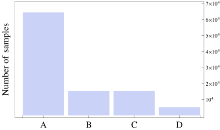
Figure 1: Distribution of the global minima of $10^{5}$ randomly generated samples. There are only four possible types of minima A, B, C and D (see Tab. 1). Type A is the one conventionally adopted to generate tiny neutrino masses in the model. The other types of minima strongly contradict the experimental facts. Nevertheless they are possible to emerge, as shown in this figure, depending on the potential parameters.

Note that the sum of the numbers in (47) equals to the total number $N=10^{5}$ , i.e.

$$\sum_{X=A,B,C,D}N_{X}=N,$$ (48)

which implies that among the $10^{5}$ samples, there are not any other new types of minima. So it numerically verifies the conclusion that Type A, B, C and D are the only four possible minima of the potential.

Besides, each of the four minima is possible to be the global minimum, depending on the parameters of the potential. In other words, a general potential of the Type II seesaw model does not necessarily lead to the VEVs we want to generate neutrino masses. As previously mentioned, only when the vacuum falls into the Type A minimum, it can be a successful theory in accord with experiments. From Fig. 1 we can see that Type A is the most likely to be the global minimum which implies that those parameter configurations for Type A global minima occupy the largest region in the parameter space. However, this is not enough. We would like to know where the region is, i.e. when the scalar fields will always get the VEVs we want. This will be studied in the next section.

At the end of this section, we explain some technical details used in the above numerical minimization. There have been many numerical methods of multidimensional minimization, such as Newton’s (or Quasi-Newton) method, Nelder-Mead simplex algorithm Nelder and Mead (1965), differential evolution Storn and Price (1997), etc. So far for general multivariable functions there have not been any numerical methods that can guarantee to find the global minimum. All the known methods are based on iterative algorithms and if the iteration converges at some point, it only means the point is a local minimum. To find the global minimum, in principle one can try many different initial points so that as many as possible local minima are found. If enough initial points are searched, the global minimum would be found. However, there is no criterion for how many initial points should be selected and too many initial points could be computationally very expensive.

In this work, to verify that there are only four types of minima, we only need an algorithm to find a local minimum. Whether it is global or not does not concern us at this stage. When the process is done for many ($10^{5}$) randomly generated potentials and the minima (the initial point is also randomly set for each potential) found are always in the four types, then the conclusion is verified at a very high confidence level. Going to the next stage, we want to make the program always find the global minimum. This can be done based on the verified conclusion that there are only four types of minima, which have been analytically computed. So we only need to compare the four known local minima to get the global minimum. Therefore, improved by the analytical result, the program can always find the global minimum.

Finally, there is something non-trivial about the parameter space. The parameters of the potential can not be arbitrary real numbers because the potential must be bounded from below (BFB). In Refs. Arhrib et al. (2011); Bonilla et al. (2015) the BFB constraint has been studied and the necessary and sufficient constraint has a slightly complicated form Bonilla et al. (2015). Besides, there are also some unitarity constraints which require those $\lambda$’s ($\lambda$ and $\lambda_{1,2,3,4}$) and their combinations not larger than some certain values, typically $4\pi$. But this is not relevant here because an overall rescaling of all the $\lambda$’s can not change the properties of the minima. So in this work, we simply take all the $\lambda$’s in the interval from $-1$ to $1$, and then reject those selections which violate the BFB constraint from Ref. Bonilla et al. (2015). As for $m$ and $M$ in the potential, since their scale is also not important, we set $M=1$ and $m\in(0,10)$. The BFB condition from Ref. Bonilla et al. (2015) is actually checked again in the numerical minimization because the iteration would not converge if the potential is not bounded from below. So this verifies that the BFB constraint from Ref. Bonilla et al. (2015) is at least sufficient.

IV From local to global

As we have seen in Fig. 1, the potential of the Type II seesaw model does not necessarily lead to the VEVs corresponding to the Type A minimum. If the Type A minimum is not the deepest (i.e. the global minimum), then there is a danger that the early universe might fall into a deeper minimum by quantum tunneling, which could be very different from the universe we are living in today. So we would like to know when the Type A minimum is global.

Since there are only four types of minima, we can compare the Type A minimum with other minima by their potential values. If the Type A minimum is deeper than all the other minima, then it must be the global minimum. The result of such an comparison (analyses given afterwards) is that, to make the Type A minimum global, we need some constraints on the potential parameters, given by

$${\rm condition\thinspace B}:\thinspace\lambda+2\eta^{2}\lambda_{1}\geq 0\quad{\rm or}\quad\lambda_{1}+2\eta^{2}\left(\lambda_{2}+\lambda_{3}\right)\leq 0,$$ (49)

$${\rm condition\thinspace C}:\thinspace\lambda+2\eta^{2}\left(\lambda_{1}+\lambda_{4}\right)\geq 0\quad{\rm or}\quad\lambda_{1}+2\eta^{2}\left(\lambda_{2}+\lambda_{3}\right)+\lambda_{4}\leq 0,$$ (50)

$${\rm condition\thinspace D}: 4\lambda_{3}\left(2\lambda_{1}+2\eta^{2}\left(2\lambda_{2}+\lambda_{3}\right)+\lambda_{4}\right)\leq 0$$ (51)

$${\rm or}\quad \left(\lambda+2\eta^{2}\lambda_{1}\right)\lambda_{3}\geq\lambda_{4}\left(\lambda_{1}+2\eta^{2}\lambda_{2}+\lambda_{4}\right)$$

$${\rm or}\quad \left(\lambda_{1}+2\eta^{2}\lambda_{2}\right)\lambda_{4}+\lambda_{3}\left(\lambda+2\eta^{2}\left(\lambda_{1}+\lambda_{4}\right)\right)\geq 0,$$

where $\eta\equiv m/M$ and condition X comes from the comparison of Type A with Type X minima. When the parameters satisfy all these conditions, then the Type A minimum must be global, as shown in Fig. 2. Similar to Fig. 1, in Fig. 2 we first randomly generated $10^{5}$ sets of parameters allowed by the BFB condition. The difference is that before minimization, we drop some of the samples that violate the above conditions.

For example, if we drop the samples that violate condition D, then after numerical minimization we find all the minima are of Type A, B or C, i.e. none of them falls into Type D, as shown in plot (i) of Fig. 2. If we drop those samples that violate condition C (or B) but not condition D, then we get plot (ii) [or plot (iii)]. If all these constraint are applied, i.e. we remove those samples that violate any of the three conditions, then the remaining samples always fall into Type A minima, shown in plot (iv). Therefore, if the parameters satisfy all the conditions given by (49)-(51), the global minimum of such a potential must be of Type A.

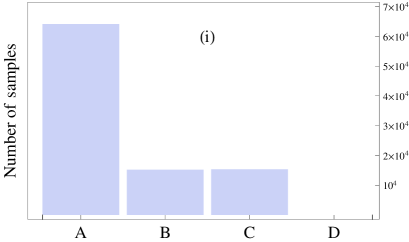
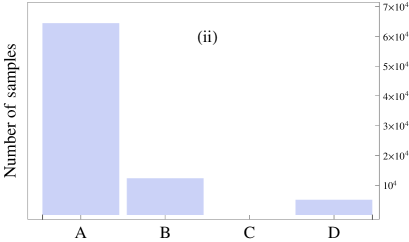
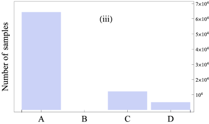
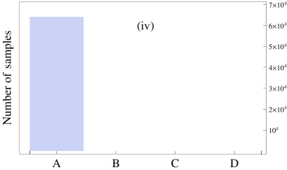
Figure 2: Similar plots to Fig. 1 but the potential parameters are constrained by conditions B, C and D given by (49)-(51). Partially adding these constraints will avoid Type D, C, or B minima being global, shown in plots (i), (ii) or (iii) respectively. Combining all of them leads to plot (iv) where all the global minima are of Type A.

Next we shall derive the conditions (49)-(51) from the comparison. Although there are analytic expressions for the four solutions in Tab. 1, for a certain set of parameters some of them may not be real solutions because $h^{2}$, $x^{2}$, $y^{2}$ or $z^{2}$ from these solutions could be negative, implying $h$, $x$, $y$ or $z$ would be imaginary at these points. So before comparing the Type A minimum with other minima, we first need to make it clear when they are real solutions.

Type A is fine in any case since $\frac{4m^{2}}{\lambda}>0$. Here $\lambda>0$ is required by the BFB condition Arhrib et al. (2011); Bonilla et al. (2015). Type B is more complicated, because whether $h^{2}$ and $z^{2}$ are positive or not depends on the denominator $\lambda_{1}^{2}-\lambda\left(\lambda_{2}+\lambda_{3}\right)$. But the BFB condition only requires Arhrib et al. (2011)

$$\lambda_{1}\geq-\sqrt{\lambda(\lambda_{2}+\lambda_{3})},$$ (52)

which can not tell us whether $\lambda_{1}^{2}-\lambda\left(\lambda_{2}+\lambda_{3}\right)$ is negative or positive. Actually the potential is bounded from below if and only if the matrix of quartic couplings is copositive Kannike (2012); Chakrabortty et al. (2014). In the case of Type B, the matrix is

$$Q_{B}=\left(\begin{array}[]{cc}\frac{\lambda}{16}&\frac{\lambda_{1}}{4}\\ \frac{\lambda_{1}}{4}&\lambda_{2}+\lambda_{3}\end{array}\right).$$ (53)

If $Q_{B}$ is positive definite, which requires that

$$\det Q_{B}=-\frac{\lambda_{1}^{2}-\lambda(\lambda_{2}+\lambda_{3})}{16}>0,$$ (54)

then for any $2\times 1$ vector $u$ we always have $u^{T}Q_{B}u>0$. In this case, the potential is always bounded from below. However, $Q_{B}$ being positive definite is a sufficient but not necessary condition of BFB. Since $u=(h^{2},\thinspace z^{2})^{T}$ only contains positive components, if all the entries of $Q_{B}$ are positive, then we still have $u^{T}Q_{B}u>0$. So the potential is bounded from below either if $Q_{B}$ is positive definite, or if all the entries of $Q_{B}$ are positive. It can be checked that this is the necessary and sufficient condition Kannike (2012). But if all the entries are positive, then the numerators in Eqs.(27) and (28) should be positive , i.e. $M^{2}\lambda_{1}+2m^{2}\left(\lambda_{2}+\lambda_{3}\right)>0$ and $M^{2}\lambda+2m^{2}\lambda_{1}>0$, which implies $h^{2}z^{2}<0$ and thus the Type B solution can not be real, no matter $\lambda_{1}^{2}-\lambda(\lambda_{2}+\lambda_{3})>0$ or not. So only the remaining case that $Q_{B}$ is positive definite concerns us. For positive definite $Q_{B}$, since $\lambda_{1}^{2}-\lambda(\lambda_{2}+\lambda_{3})<0$, if $M^{2}\lambda_{1}+2m^{2}\left(\lambda_{2}+\lambda_{3}\right)>0$ and $M^{2}\lambda+2m^{2}\lambda_{1}<0$, then we have positive $h^{2}$ and $z^{2}$ for the Type B solution. Note that $\lambda_{1}$ can not be positive if the two numerators have opposite signs, thus we can draw the conclusion that as long as the potential is bounded from below, the Type B solution is real if and only if $M^{2}\lambda_{1}+2m^{2}\left(\lambda_{2}+\lambda_{3}\right)>0$ and $M^{2}\lambda+2m^{2}\lambda_{1}<0$.

If this condition is satisfied, then we need to compare the potential values at the Type A and B minima, denoted as $V_{0}^{(A)}$ and $V_{0}^{(B)}$ respectively. By straightforward calculation, the difference $V_{0}^{(A)}-V_{0}^{(B)}$ is

$$V_{0}^{(A)}-V_{0}^{(B)}=\frac{M^{4}\left(\lambda+2m^{2}\lambda_{1}\right){}^{2}}{4\lambda\left(-\lambda_{1}^{2}+\lambda(\lambda_{2}+\lambda_{3})\right)},$$ (55)

which is positive if $\lambda>0$ and $-\lambda_{1}^{2}+\lambda(\lambda_{2}+\lambda_{3})>0$. $\lambda>0$ can be guaranteed by the BFB condition while $-\lambda_{1}^{2}+\lambda(\lambda_{2}+\lambda_{3})>0$ is satisfied as long as the Type B solution is real, explained as follows. As just mentioned, if Type B is real, then it excludes the possibility of positive $\lambda_{1}$, otherwise $h^{2}z^{2}$ would be negative. Then from (52) we have $-\lambda_{1}^{2}+\lambda(\lambda_{2}+\lambda_{3})>0$. So if the Type B solution is real then the potential value at the Type B minimum must be lower than Type A. To avoid that, we need to add some constraints so that the real Type B solution can not exist. Therefore either the condition $M^{2}\lambda_{1}+2m^{2}\left(\lambda_{2}+\lambda_{3}\right)>0$ or $M^{2}\lambda+2m^{2}\lambda_{1}<0$ should be violated, which gives the result given by (49).

Next let us turn to the Type C solution. The analysis is similar and we find that the Type C solution is real if and only if $2m^{2}\left(\lambda_{2}+\lambda_{3}\right)+M^{2}\left(\lambda_{1}+\lambda_{4}\right)>0$ and $M^{2}\lambda+2m^{2}\left(\lambda_{1}+\lambda_{4}\right)<0$. The difference $V_{0}^{(A)}-V_{0}^{(C)}$ where $V_{0}^{(C)}$ is the potential value at the Type C minimum is

$$V_{0}^{(A)}-V_{0}^{(C)}=\frac{M^{4}\left(\lambda+2m^{2}\left(\lambda_{1}+\lambda_{4}\right)\right){}^{2}}{4\lambda\left(\lambda\left(\lambda_{2}+\lambda_{3}\right)-\left(\lambda_{1}+\lambda_{4}\right){}^{2}\right)}.$$ (56)

Again, this implies that to avoid a deeper minimum at Type C, we need to break the existence condition of the real Type C solution, which leads to the result given by (50).

Finally there is the Type D solution. Though it has the most complicated form, we find that the analysis is still similar. The difference $V_{0}^{(A)}-V_{0}^{(D)}$ can be written as

$$V_{0}^{(A)}-V_{0}^{(D)}=\frac{M^{4}\left(\lambda+2m^{2}\lambda_{1}\right){}^{2}}{4\lambda\left(\lambda\left(\lambda_{2}+\lambda_{3}\right)-\lambda_{1}^{2}\right)}+\frac{M^{4}\left(\left(\lambda_{1}+2m^{2}\lambda_{2}\right)\lambda_{4}+\lambda_{3}\left(\lambda+2m^{2}\left(\lambda_{1}+\lambda_{4}\right)\right)\right){}^{2}}{8\det Q\left(\lambda\left(\lambda_{2}+\lambda_{3}\right)-\lambda_{1}^{2}\right)},$$ (57)

where $\det Q$ has been defined in Eq.(40). Again, the denominators are positive because those determinants are positive. The numerators are positive because they are in squared forms. So a similar analysis gives the result in (51).

V To The NLO

The above analysis is only for the LO, i.e. assuming $\mu=0$. However, in the limit of zero $\mu$, the model can not account for tiny neutrino masses. In this section, we will introduce a perturbatively small but nonzero $\mu$ into our calculation, to see how those local minima are modified by the NLO correction.

First we would like to discuss in general the perturbative calculation near minima. Consider a general potential $V(\phi)$ which is a function of multifields $\phi=(\phi_{1},\phi_{2},\cdots)$ and can be written as

$$V(\phi)=V_{0}(\phi)+\delta V(\phi),$$ (58)

where $V_{0}$ and $\delta V$ are the LO and NLO terms. Assume that $V_{0}$ has a minimum at $\phi^{(0)}$, i.e.

$$\left.\frac{\partial V_{0}}{\partial\phi_{i}}\right|_{\phi=\phi^{(0)}}=0,\thinspace\thinspace(i=1,2,3\cdots),$$ (59)

then the corresponding minimum of $V$, computed at the NLO should be approximately at

$$\phi^{(1)}=\phi^{(0)}+\delta\phi,$$ (60)

where $\delta\phi$ can be determined from

$$\delta\phi=-\left.\left[\frac{\partial^{2}V_{0}}{\partial\phi_{i}\partial\phi_{j}}\right]^{-1}\frac{\partial\delta V}{\partial\phi}\right|_{\phi=\phi^{(0)}}.$$ (61)

The potential value at this minimum is

$$V(\phi^{(1)})=V_{0}(\phi^{(0)})+\delta V(\phi^{(0)})+O(\delta\phi^{2}).$$ (62)

Here we briefly derive Eqs. (61) and (62). Consider the equation $\partial V/\partial\phi=0$, which is

$$\left.\frac{\partial V_{0}(\phi)}{\partial\phi_{i}}+\frac{\partial\delta V(\phi)}{\partial\phi_{i}}\right|_{\phi=\phi^{(0)}+\delta\phi}=0.$$ (63)

The first term can be expanded as

$$\left.\frac{\partial V_{0}(\phi)}{\partial\phi_{i}}\right|_{\phi=\phi^{(0)}+\delta\phi}=\left.\frac{\partial V_{0}(\phi)}{\partial\phi_{i}}\right|_{\phi=\phi^{(0)}}+\delta\phi_{j}\left.\frac{\partial^{2}V_{0}}{\partial\phi_{i}\partial\phi_{j}}\right|_{\phi=\phi^{(0)}}+O(\delta\phi^{2}),$$ (64)

while the second term of Eq. (63) is

$$\left.\frac{\partial\delta V(\phi)}{\partial\phi_{i}}\right|_{\phi=\phi^{(0)}+\delta\phi}=\left.\frac{\partial\delta V(\phi)}{\partial\phi_{i}}\right|_{\phi=\phi^{(0)}}+O(\delta\phi^{2}).$$ (65)

Using Eq. (59) we write Eq. (63) as

$$\delta\phi_{j}\left.\frac{\partial^{2}V_{0}}{\partial\phi_{i}\partial\phi_{j}}\right|_{\phi=\phi^{(0)}}+\left.\frac{\partial\delta V(\phi)}{\partial\phi_{i}}\right|_{\phi=\phi^{(0)}}+O(\delta\phi^{2})=0.$$

which is a linear equation of $\delta\phi$. Solving the equation, we get Eq. (61). Eq. (62) can be obtained by directly expanding the potential value near the LO minimum. Because $\partial V_{0}/\partial\phi$ at the LO minimum is zero and $\delta V(\phi^{(1)})=\delta V(\phi^{(0)})+O(\delta\phi^{2})$, we simply get the result in Eq. (62).

corrections	Type A	Type B	Type C	Type D
$\delta h/\mu$	0	0	$\frac{\sqrt{-C_{1}C_{2}}\left(2C_{2}\left(\lambda_{2}+\lambda_{3}\right)+C_{1}\left(\lambda_{1}+\lambda_{4}\right)\right)}{C_{d}C_{1}C_{2}}$	$\frac{\sqrt{-D_{1}D_{2}}\lambda_{3}\left(D_{1}\lambda_{1}+10D_{2}\lambda_{2}+2D_{3}\lambda_{2}-4D_{3}\lambda_{3}+3D_{1}\lambda_{4}\right)}{\sqrt{2}D_{d}D_{1}D_{2}}$
$\delta x/\mu$	$\frac{2m^{2}}{C_{2}}$	$\frac{B_{1}}{B_{2}\lambda_{3}+B_{1}\lambda_{4}}$	$-\frac{m^{2}}{C_{2}}-\frac{3\left(\lambda_{1}+\lambda_{4}\right)}{2C_{d}}$	$\frac{D_{1}\lambda_{1}^{2}-\lambda D_{1}\left(\lambda_{2}+\lambda_{3}\right)-4D_{2}\left(\lambda_{1}\lambda_{3}+\lambda_{2}\lambda_{4}+\lambda_{3}\lambda_{4}\right)}{4D_{2}D_{d}}$
$\delta y/\mu$	0	0	0	0
$\delta z/\mu$	0	0	0	$\frac{\sqrt{-D_{2}D_{3}}\left(-D_{1}\lambda_{1}^{2}+\lambda D_{1}\lambda_{2}+4D_{3}\lambda_{1}\lambda_{3}-3D_{1}\lambda_{1}\lambda_{4}+4D_{2}\lambda_{2}\lambda_{4}\right)}{4D_{d}D_{2}D_{3}}$
$\delta V_{{\rm min}}/\mu$	0	0	$-\sqrt{\frac{-C_{2}}{C_{d}}}\frac{\sqrt{2}C_{1}}{C_{d}}$	$-\sqrt{\frac{-D_{2}}{D_{d}}}\frac{D_{1}}{\sqrt{2}D_{d}}$

Table 2: NLO corrections of the solutions listed in Tab. 1.

With Eqs. (61) and (62), it is quite straightforward to compute the NLO corrections. The result is listed in Tab. 2, where $B_{1,2,d}$, $C_{1,2,d}$ and $D_{1,2,3,d}$ are defined below,

$$B_{1}=M^{2}\lambda_{1}+2m^{2}\left(\lambda_{2}+\lambda_{3}\right),$$ (66)

$$B_{2}=M^{2}\lambda+2m^{2}\lambda_{1},$$ (67)

$$B_{d}=\lambda\left(\lambda_{2}+\lambda_{3}\right)-\lambda_{1}^{2},$$ (68)

$$C_{1}=2m^{2}\left(\lambda_{2}+\lambda_{3}\right)+M^{2}\left(\lambda_{1}+\lambda_{4}\right),$$ (69)

$$C_{2}=M^{2}\lambda+2m^{2}\left(\lambda_{1}+\lambda_{4}\right),$$ (70)

$$C_{d}=\lambda\left(\lambda_{2}+\lambda_{3}\right)-\left(\lambda_{1}+\lambda_{4}\right){}^{2},$$ (71)

$$D_{1}=2\lambda_{3}\left(2m^{2}\left(2\lambda_{2}+\lambda_{3}\right)+M^{2}\left(2\lambda_{1}+\lambda_{4}\right)\right),$$ (72)

$$D_{2}=\left(M^{2}\lambda_{1}+2m^{2}\lambda_{2}\right)\lambda_{4}+\lambda_{3}\left(M^{2}\lambda+2m^{2}\left(\lambda_{1}+\lambda_{4}\right)\right),$$ (73)

$$D_{3}=\lambda_{4}\left(2m^{2}\lambda_{2}+M^{2}\left(\lambda_{1}+\lambda_{4}\right)\right)-\left(M^{2}\lambda+2m^{2}\lambda_{1}\right)\lambda_{3},$$ (74)

$$D_{d}=\lambda_{3}\left(-2\lambda_{1}^{2}+\lambda\left(2\lambda_{2}+\lambda_{3}\right)\right)-2\lambda_{1}\lambda_{3}\lambda_{4}-\left(\lambda_{2}+\lambda_{3}\right)\lambda_{4}^{2}.$$ (75)

An interesting point is that even in the NLO correction, $y$ still remains zero. That is to say, the diagonal entries of $\Delta$ always acquire zero VEVs. Besides, the NLO correction to $V_{{\rm min}}$ is zero for Type A and B minima. The reason is that the NLO correction to $V_{{\rm min}}$ is proportional to the value of $x^{2}$ at LO, which is zero for the Type A and B minima (cf. Tab. 1).

In the LO calculation, we have obtained the condition of the Type A minimum being the global minimum. So we would like to know the corresponding condition at the NLO. The method is the same as what we have done in the LO analysis. Because we have the analytic expressions for all the minima at the NLO, one may simply compare the four types of minima at the NLO to find the global minimum. However, we find that the explicit expression of the condition to keep the Type A minimum global at the NLO is very complicated, since the explicit forms of the NLO solutions are already very complicated, as one can see from Eqs. (66)-(75) and Tab. 2. So in practical use, to check if the potential has the Type A global minimum for a set of numerically given parameters, we would recommend evaluating the expressions in Tab. 1 and Tab. 2 directly and comparing the four minima, instead of using more complicated expressions derived from them.

VI Predictions of the mass splitting

After spontaneous symmetry breaking, there are five massive scalar fields in the Type II seesaw model, including three neutral fields $(h^{0},\thinspace H^{0},\thinspace A^{0})$, one singly-changed field $H^{\pm}$ and one doubly-changed field $H^{\pm\pm}$. Apart from the five scalar masses, the vacuum expectation values $(v_{H},\thinspace v_{\Delta})$ and the mixing angle $\alpha$ between $h^{0}$ and $H^{0}$ are also physical observables. The 8 physical observables can be used to reconstruct the parameters in the potential, since the potential only has 8 parameters $(m^{2},\thinspace M^{2},\thinspace\mu,\thinspace\lambda,\thinspace\lambda_{1,2,3,4})$. For explicit expressions, see Ref. Arhrib et al. (2011). Conversely, the 8 physical observables can also be expressed in terms of the 8 potential parameters, which enable us to convert constraints on the potential parameters to physical predictions.

For simplicity, we only focus on the predictions of the scalar mass spectrum. In the Type II seesaw model, usually $h^{0}$ is considered as the Higgs boson with mass $m_{h^{0}}=125$ GeV that has been discovered at the LHC since 2012 Aad et al. (2012); Chatrchyan et al. (2012). The other massive scalar bosons are assumed to be much heavier than $h^{0}$. At the LO, their masses are given by Arhrib et al. (2011)

$$m_{H^{\pm}}^{2}=M^{2}+\left(2\lambda_{1}+\lambda_{4}\right)\frac{v_{H}^{2}}{4}+{\cal O}(\mu^{2}),\thinspace\thinspace m_{H^{\pm\pm}}^{2}=M^{2}+\lambda_{1}\frac{v_{H}^{2}}{2}+{\cal O}(\mu^{2}),$$ (76)

$$m_{A}^{2}=M^{2}+\left(\lambda_{1}+\lambda_{4}\right)\frac{v_{H}^{2}}{2}+{\cal O}(\mu^{2}),\thinspace\thinspace m_{H^{0}}^{2}=M^{2}+\left(\lambda_{1}+\lambda_{4}\right)\frac{v_{H}^{2}}{2}+{\cal O}(\mu^{2}),$$ (77)

which implies that if the Type II seesaw scale $M$ is much higher than the electroweak scale $v_{H}$, then all the four bosons should have masses approximately equal to $M$. However, there are still mass splittings among them. Defining

$$\Delta m^{2}\equiv m_{H^{0}}^{2}-m_{H^{\pm\pm}}^{2},$$ (78)

we find that

$$\Delta m^{2}\approx m_{A}^{2}-m_{H^{\pm\pm}}^{2}\approx 2(m_{H^{\pm}}^{2}-m_{H^{\pm\pm}}^{2})\approx\frac{\lambda_{4}}{2}v_{H}^{2}.$$ (79)

There is yet another much smaller mass squared difference,

$$\delta m^{2}\equiv m_{A}^{2}+m_{H^{\pm\pm}}^{2}-2m_{H^{\pm}}^{2}\approx(\lambda_{4}-\lambda_{3})v_{\Delta}^{2}.$$ (80)

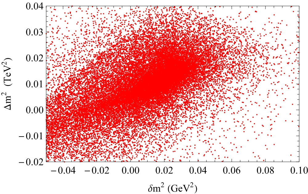
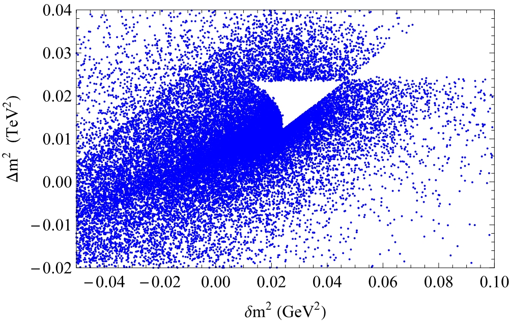
Figure 3: The allowed region of the mass splitting parameters $\Delta m^{2}\equiv m_{H^{0}}^{2}-m_{H^{\pm\pm}}^{2}$ and $\delta m^{2}\equiv m_{A}^{2}+m_{H^{\pm\pm}}^{2}-2m_{H^{\pm}}^{2}$ with (blue) or without (red) the requirement of the Type A vacuum being the deepest.

If the potential is required to have the Type A global minimum, then there may be additional constraints on $\delta m^{2}$ and $\Delta m^{2}$. We use random search to find the constraints numerically, as shown in Fig. 3. In the left panel, we randomly generate $4\times 10^{4}$ samples with all the potential parameters subject to the BFB constraint from Ref. Bonilla et al. (2015) and compute the corresponding values of $\delta m^{2}$ and $\Delta m^{2}$ while in the right panel, the samples are further constrained by Eqs. (49)-(51). To make it realistic, we fix the Higgs mass $m_{h^{0}}$ at 125 GeV, and $v=\sqrt{v_{H}^{2}+v_{\Delta}^{2}}$ at 246 GeV. Also we assume $m_{H^{0}}$ should be heavy ($m_{H^{0}}=$1 TeV) while $v_{\Delta}$ and $\alpha$ should be small ($v_{\Delta}=0.245$ GeV, $\tan 2\alpha=4\times 10^{-3}$). Thus, the potential parameters are also subject to these constraints. As we can see, there is a difference between the left and right panels in Fig. 3: in some region of the right panel blue points do not appear, which implies that the corresponding values of $(\delta m^{2},\thinspace\Delta m^{2})$ are not allowed if the Type A minimum is global.

VII Conclusion

In the Type II seesaw model, the vacuum could be of four different types, namely Type A, B, C and D. The analytic expressions of the VEVs are listed in Tab. 1 for the LO and Tab. 2 for the NLO. Among the four vacua only one of them, the Type A vacuum, is allowed by the experimental facts such as tiny neutrino masses, unbroken $U(1)_{{\rm em}}$, etc. However, the most general scalar potential in the model does not necessarily lead to the Type A vacuum, because it generally has several different local minima and sometimes the Type A minimum is not the deepest. In Fig. 1 we see that among the $10^{5}$ randomly generated samples, the Type A minimum appears as the global minimum in about $64\%$ of them, i.e. for the remaining $36\%$ the Type A minimum is not the deepest. If several deeper vacua coexist with it, the Type A vacuum could be unstable since it would decay into other deeper vacua via quantum tunneling.

Therefore, it is important to know when the Type A vacuum is the deepest one. We have found the condition for it, given by Eqs. (49)-(51). If the potential parameters are constrained by this condition, then the Type A minimum must be the global minimum and the stability is guaranteed. As one can see from Fig. 2, when the condition is partially added, the vacuum can be avoided to be of Type B, C or D; when the condition is fully added, the vacuum must be of Type A. An interesting physical consequence of this condition is that it will lead to predictions on the mass splitting of the heavy bosons, as shown in Fig. 3.

Note that the absolute stability of the Type A vacuum might be a too strong constraint on the model. Although it might decay into a deeper minimum by quantum tunneling if it was not the deepest, the model could still be valid since the decay rate could be low enough so that the lifetime of the vacuum would be longer than the age of the universe Coleman (1977); Callan and Coleman (1977). That is, the vacuum could be meta-stable. So to see whether there is the vacuum-instability problem for a certain set of parameters, one has to compute the decay rate. However, this could be much more complicated and is out of scope of the current paper. For simplicity, we only consider that the Type A minimum by itself is the deepest point of the potential so that the decay rate will not concern us. Besides, if we obtain the absolute stability condition, there is no longer a need to check the second derivatives of the potential to guarantee that the extremum is a local minimum, not a saddle point or a local maximum. Once the potential satisfies the condition that the Type A minimum is the deepest point, then combined with the bounded-from-below condition the Hessian matrix must be positive (semi-)definite at the point. Therefore, though it is a little too strong, the requirement of absolute stability may be the simplest way to construct a valid scalar potential for the model concerned with the above issues.