Recurrent Image Captioner: Describing Images with Spatial-Invariant Transformation and Attention Filtering

Abstract

Along with the prosperity of recurrent neural network in modelling sequential data and the power of attention mechanism in automatically identify salient information, image captioning, a.k.a., image description, has been remarkably advanced in recent years. Nonetheless, most existing paradigms may suffer from the deficiency of invariance to images with different scaling, rotation, etc.; and effective integration of standalone attention to form a holistic end-to-end system. In this paper, we propose a novel image captioning architecture, termed Recurrent Image Captioner (RIC), which allows visual encoder and language decoder to coherently cooperate in a recurrent manner. Specifically, we first equip CNN-based visual encoder with a differentiable layer to enable spatially invariant transformation of visual signals. Moreover, we deploy an attention filter module (differentiable) between encoder and decoder to dynamically determine salient visual parts. We also employ bidirectional LSTM to preprocess sentences for generating better textual representations. Besides, we propose to exploit variational inference to optimize the whole architecture. Extensive experimental results on three benchmark datasets (i.e., Flickr8k, Flickr30k and MS COCO) demonstrate the superiority of our proposed architecture as compared to most of the state-of-the-art methods.

1 Introduction

Advanced by the rapid development of smart mobile devices, massive storage, fast Internet and prevailing social media sharing platforms, we have witnessed a tremendous explosion of image data on the Web. Visual content understanding has been long studied in literature, ranging from object recognition [20, 36, 8], to image classification [20, 30], to visual semantic analysis [56, 57, 61, 23, 3]. Recently, the research focus has gradually shifted to the more challenging visual task, i.e., image captioning, which refers to the process of generating meaningful natural language description for image data, towards deep understanding of visual content. Beside the basic recognition/detection of visual participants, image captioning further explores their interrelationships, which inevitably poses more non-trivial challenges on the model design.

Existing image captioning approaches can be roughly categorized into two schemes: 1) template-based approaches [32] and 2) neural network based approaches [26]. Most of the early attempts focus on the the former family of captioning methods, which discover static visual participants (e.g., objects, scenes) from images first and then fit them into the templates prepared beforehand. Nonetheless, such approaches are prone to “general” descriptions while ignoring the specifics, e.g., the location information. During the past few years, because of the overwhelming data modeling power of deep learning, the state-of-the-art captioning performance has been dominated by neural network based approaches [5, 11, 39], which “mimic” machine translation to transform images (CNN-based encoder) into sentences (LSTM-based decoder) in an end-to-end system. One limitation of such paradigms is that they heavily depend on the entire visual representations of images, thereby neglecting the fine-grained details due to the complexity and arbitrariness of image content.

Intuitively, when watching a piece of image, one might only attend to a small proportion of objects among various participants, e.g., the leading character among all the actors in a single screen. Inspired by this observation, attention mechanism [54, 44] has been introduced to facilitate the encoder-decoder framework to explore more detailed aspects. By simulating human visual perception system, attention tries to identify certain particular salient parts of a given image and has successfully facilitated a variant of applications, such as image generation [19] and object detection [62]. In [54], the description generating process condition on the hidden states images encoder, rather than on one single context vector only, that is to selectively attend to parts of the scene while ignoring others.

It is known that a commonly-used choice of visual encoder is traditional Convolutional Neural Network (CNN), which provides limited support for exploring spatial invariant property in input images [24]. Hence, this drawback may cause the encoder-decoder framework vulnerable to images with large variance, such as scaling, rotation, translation, etc. Besides, existing attention mechanism normally serves as a standalone component (e.g., select feature maps from a fixed some low levels map of a pretrained CNN layers to represent images [54]) attached to certain encoder-decoder framework, which cannot be formulated as a holistic end-to-end system for coherently unifying the processes of visual encoding, attending to salient parts and decoding to sentences.

In this paper, we propose a novel architecture, termed Recurrent Image Captioner (RIC), which unifies spatially invariant property, automatical attention filtering mechanism together with a recurrent feedback loop between CNN-based encoder and LSTM-based decoder to form an end-to-end formulation for image captioning task. Specifically, inspired by [24], we first equip CNN-based visual encoder with a differentiable layer to enable spatially invariant transformation of visual signals. Then, in order to achieve indepth integration of attention mechanism, we add a differentiable attention filter to automatically capture the semantically vital regions in a dynamic manner based on previous visual representations and generated captions. Besides, due to the sequential nature of image description and generation process, we further introduce a loop from decoder to spatial transformation layer to feedback the invariant information in a recurrent way. The recurrent feedback loop helps to gradually bridge the semantic gap between low-level visual features and high-level caption semantics, thereby generating more accurately captions by translating the spatially invariant visual signals filtered by the attention module. For optimization, there are plenty of sequential attention models trained with reinforcement learning techniques, such as policy gradients [44]. It is worth noting that both of the aforementioned components are differentiable, which makes our proposed RIC architecture easy to optimize with standard backpropagation. We propose to exploit variational inference [15] to optimize the whole architecture.

We summarize our contributions as follows:

• We propose a novel image captioning architecture, which formulates the processes of visual encoding, spatial transformation, attention filtering as well as sentence decoding in a recurrent feedback loop.

• Both the spatial transformation layer and attention filter are differentiable, which makes the whole structure easy to optimize with the assistance of variational inference.

• Extensive experiments on Flickr8k, Flickr30k and MS COCO datasets demonstrate the superiority of our proposal as compared to the state-of-the-arts.

The rest of this paper is organized as below. Section 2 briefly reviews related work on image captioning. Section 3 elaborated the proposed Recurrent Image Captioner. In Section 4, we report experiments on three image benchmarks, followed by the conclusion in Section 5.

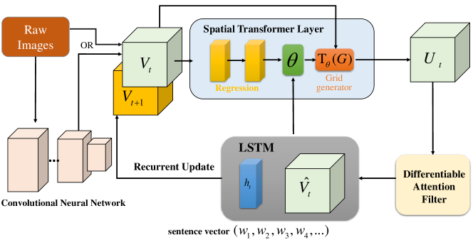
Figure 1: The overall flowchart of the proposed Recurrent Image Captioner architecture.

2 Related Work

In this section, we briefly review related work on image captioning and attention mechanism. Generally, existing captioning can be roughly categorized into two families: template-based approaches  [12, 33] and neural network based approaches [25, 26, 54]. Most of the early attempts focus on the the former family of captioning methods, which discover static visual participants (e.g., objects, scenes) from images first and then fit them into the templates prepared beforehand. For instance, in [14, 31], semantic concepts are detected and then fed into templates to construct sentences. In  [35] concepts are first discovered and then directly combined together. Nonetheless, such approaches are prone to “general” descriptions while ignoring the specifics, e.g., the location information.

Recently, various neural network based methods have been proposed for generating image descriptions. The very first approach to use neural network to generating image caption generation neural work was [28], which introduces a multimodal log-bilinear model biased by features from the image. This work was then followed by [29] in which an explicit way of ranking and generation was introduced. There are also recurrent neural network based approaches to image caption generation, such as [1, 7, 11, 49, 52], where a commonly used RNN structure is a LSTM. They represent images as a single feature vector from the top layer of a pre-trained convolutional network. [40] proposes to learn a joint embedding space of both images and descriptions for ranking and caption generation. The model learns to score sentence and image similarity as a function of R-CNN object detections with outputs of a bidirectional RNN. [13] proposes a three-step pipeline for generation by incorporating object detections. Recently, we have witnessed an increasing trend of incorporating attention mechanism [13, 25, 29, 52, 54] into neural networks for boosting computer vision and artificial intelligence tasks, such as object recognition, image caption, etc. There are also attention based work to handle semantic related tasks, such as [13].

In comparison to existing approaches, it is important to note that our proposed architecture introduce two differentiable modules, which enables our method capturing global information in images and learning spatially invariant structure in a holistic end-to-end system. Furthermore, we show the benefit of our architecture by defining a variational loss function which employs an autoencoder to regularize the process of image captioning.

3 Recurrent Image Captioner

In this section, we elaborate the details of the proposed Recurrent Image Captioner, including architecture overview, spatial transformation layer, differential attention filter as well as loss functions.

3.1 Architecture Overview

The overall flowchart of our proposed RIC is illustrated in Fig. 1, which comprises four major components: (a) basic CNN encoder, (b) spatial transformation layer, (c) differentiable attention filter and (d) language decoders. Given a set of training images, we feed them into the CNN encoder, which outputs visual latent codes, denoted as $V_{t}$. Then, the spatial transformation layers converts the visual latent codes into spatially invariant signals, denoted as $U_{t}$, which are subsequently passed to the attention filter to distill the most semantically informative parts. The conventional LSTM is then employed to decode the filtered signals to sentences. After after a duration of steps, the decoding outputs are successively added to the distribution that generates the captions rather than emitting a word in a single step. This shows that our method capture more higher concept instead of simple word-level information in image. Finally, we recurrently feedback the output parameters of the decoder for updating the visual latent codes and the transformation parameter $\theta$.

3.1.1 Basic CNN Encoder

Following conventions, we use CNN as encoder as well. Specifically, we employ VGG-16 [48] to extract a set of visual feature vectors for a given image, denoted as

$$\mathcal{A}=\{{a_{1}},{a_{2}},\cdots,{a_{L}}\},$$ (1)

where each ${a_{i}}\in{\mathbb{R}^{d}}$ corresponds to a part of the image, $L$ is the number of image parts and $d$ is the dimensionality of the feature space.

3.1.2 Basic LSTM Decoder

For better decoding, we propose to preprocess image captions with Bidirectional LSTM . In a Bidirectional LSTM model, the two LSTMs [21] jointly process the input caption sequence from both forward and backward directions. The forward LSTM computes the sequence of forward hidden states, denoted as $\{\vec{w}_{1},\vec{w}_{2},...,\vec{w}_{M}\}$, whereas the backward LSTM computes the sequence of backward hidden states $\{\vec{w^{\prime}}_{1},\vec{w^{\prime}}_{2},...,\vec{w^{\prime}}_{M}\}$, where $M$ is the number of words in the caption. These hidden states are then concatenated together into the sequence $\mathcal{W}=[w_{1},w_{2},...,w_{M}]$, with $w_{i}=[\vec{w}_{i},\vec{w^{\prime}}_{i}],1\leq i\leq M$. The process is illustrated in Fig. 2 for a graphical interpretation. It is worth noting that instead of representing caption with 1-of-$K$ encoded words, we can regard the bidirectional LSTM as a generator of word embedding, which is capable of capturing semantical relationships in language.

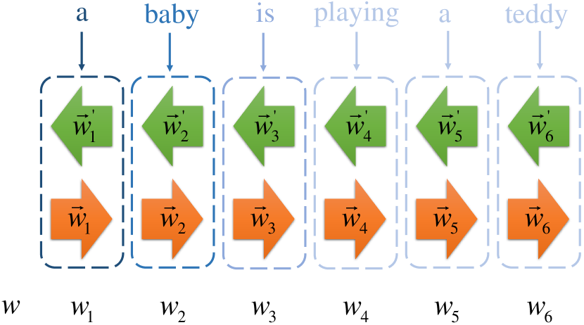
Figure 2: Illustration of Bidirectional LSTM for encoding captions.

To model the decoding process, we exploit Long Short-Term Memory architecture [21] with extension of forget gates [16] due to its excellent capability of modelling long-range dependencies in real sequential data. We follow the implementation of LSTM as in [60].

3.2 Spatial Transformation Layer

In this part, we present a spatial transformation layer extended from , which is installed on top of the CNN encoder to add spatially invariant information into visual signals. As shown in Fig. 1, different from the original model as in , the transformation parameter $\theta$ in our spatial transformation layer not only depends on the internal regression network but also conditions on the LSTM module in the decoder, which forms the foundation of the recurrent updating loop between encoder and decoder.

Suppose we are given the input feature cube $V_{t}\in{\mathbb{R}^{H\times W\times C}}$ at time step $t$, where $H$, $W$ and $C$ represents height, width and the number of channels, respectively, then we calculate the transformation parameter $\theta$ as follows:

$$\theta=f_{recurrent}(V_{t},h_{t},\hat{V}_{t}),$$ (2)

where $\hat{V}_{t}$ denotes the output of the attention filter in the $t$-th updating loop, which will be elaborated in the next subsection. $h_{t}$ is the hidden states of the LSTM-based decoder in the $t$-th updating loop. $f_{recurrent}(\cdot)$ is the recurrent updating function of the transformation parameter $\theta$. $f_{recurrent}(\cdot)$ can be implemented as a multilayer perception or as a gated activation function, such as LSTM or Gated Recurrent Unit (GRU) [7]. Both LSTM and GRU have been applied to learn long-term dependencies. In our experiments, we have found that GRU provides slightly better performance than LSTM, therefore we choose to use GRU as the implementation of $f_{recurrent}(\cdot)$.

Then we assemble the transformation, which should be differentiable, as $T_{\theta}=P_{\theta}B$, where $P_{\theta}$ is a matrix parameterised by $\theta$ and $B$ is the representation of a grid. As pointed out in , we may possibly learn to predict $\theta$, and also learn $B$ for the task.

After the transformation, we apply a learnable kernel as a mask. Here, we refer pixel to a particular location, which is not necessarily a real visual pixel.

$$\begin{array}[]{l}\hat{U}_{i,t}=\sum\limits_{m}^{H^{V}_{t}}{\sum\limits_{n}^{W^{V}_{t}}{V_{nm,t}^{c}}}k(x_{i}-m|{\Phi_{x}})k(y_{i}-n|{\Phi_{y}}),\\ \forall i\in[1,\cdots,H^{U}_{t}W^{U}_{t}],\forall c\in[1,\cdots,C]\end{array}$$ (3)

where each $(x_{i},y_{i})$ coordinate in $T_{\theta}$ defines the spatial location in the input where a kernel is applied to get the value at a particular pixel in the output $V_{i,t}^{c}$. $H_{t}^{V}$ and $W_{t}^{V}$ are the dimensions of $V^{c}_{nm,t}$ , while $H_{t}^{U}$ and $W_{t}^{U}$ are dimensions of $\hat{U}_{i,t}$. $\Phi_{x}$ and $\Phi_{y}$ are the parameters of a generic sampling kernel $k(\cdot|\cdot)$, which is differentiable. To preserve spatial consistence we apply identical sampling/transformation strategy to each channel of the input. Mask has been used in many image modeling work, such as [9, 10, 34, 42, 51]. Different from previous work, our model do not use pre-trained mask but learn a proper mask using a recurrent neural network.

3.3 Differentiable Attention Filter

In this part, we introduce the attention filtering module which serves as an important role in our architecture. Specifically, we take inspiration from the differentiable attention mechanisms for handwriting synthesis [17] and Neural Turing Machines [18, 19]. We use an array of 2-D Gaussian filters, which is an explicit 2-D form of attention map. The output of this module varies smoothly on different locations. The real-valued grid center $(g_{X},g_{Y})$ and stride $\delta$ determine the mean location $(\mu_{X}^{i},\mu_{Y}^{i})$ of the filter at row $i$, column $j$ in the patch as follows:

$$\left\{\begin{array}[]{c}\mu_{X}^{i}={g_{X}}+(i-N/2-0.5)\delta,\\ \mu_{Y}^{j}={g_{Y}}+(j-N/2-0.5)\delta,\end{array}\right.$$ (4)

where $N$ is the dimensionality of input. The isotropic variance $\sigma^{2}$ of the Gaussian filters, and a scalar intensity $\gamma$ that multiplies the filter response are defined as follows:

$$\left\{\begin{aligned} &(\hat{g}_{Y},\hat{g}_{Y},\log{\sigma^{2}},\log\hat{\delta},\log\gamma)=Ph_{t},\\ &{g_{X}}=\frac{{H_{t}^{V}+1}}{2}(\hat{g}_{X}+1),\\ &{g_{Y}}=\frac{{W_{t}^{V}+1}}{2}(\hat{g}_{Y}+1),\\ &\delta=\frac{{\max(H_{t}^{V},W_{t}^{V})-1}}{{N-1}}\hat{\delta},\end{aligned}\right.$$ (5)

where $P$ is a linear mapping matrix. Given an input image or feature map of size $N\times N$, where the variance, stride and intensity are emitted in the log-scale to ensure positivity.

The horizontal and vertical filter bank matrices $F_{X}$ and $F_{Y}$ are defined as follows:

$$\left\{\begin{array}[]{l}{F_{X}}[i,m]=\frac{1}{{{Z_{X}}}}\exp(-\frac{{{{(m-\mu_{X}^{i})}^{2}}}}{{2{\sigma^{2}}}}),\\ {F_{Y}}[j,n]=\frac{1}{{{Z_{Y}}}}\exp(-\frac{{{{(n-\mu_{Y}^{j})}^{2}}}}{{2{\sigma^{2}}}}),\end{array}\right.$$ (6)

where $(i,j)$ is a point in the attention patch, $(m,n)$ is a point in the input image, and $Z_{X},Z_{Y}$ are normalization constants that ensure $\Sigma_{m}F_{X}[i,m]$ = 1 and $\Sigma_{n}F_{Y}[j,n]$ = 1. We can view it as the process of producing two arrays of 1D Gaussian filter banks, whose filter locations and scales are computed from the LSTM hidden states. Given the above equation, we then apply this attention filter on top of spatial transformation layer.

One way is $\hat{V_{t}}$ := $\gamma F_{X}U_{t}F_{Y}^{T}$ given the previous layer output $U_{t}$. Another way is to calculate the convolution of the filter map $F_{X}$, $F_{Y}$ and $U_{t}$, followed by a pooling operation. The output of this module will serve as latent code in our variational loss function:

$$\left\{\begin{aligned} &{{\tilde{V}}_{1}^{c}}={U^{c}_{t}}*{F_{X}},~{}c=1,2,\ldots,C;\\ &{{\tilde{V}}_{2}^{c}}={{\tilde{V}}_{1}^{c}}*{F_{Y}},~{}c=1,2,\ldots,C;\\ &{\hat{V}_{t}^{c}}\leftarrow\mathbf{pool}({{\tilde{V}}^{c}_{2}}),~{}c=1,2,\ldots,C.\end{aligned}\right.$$ (7)

Here $*$ is convolution operation performed at every channel, $\mathbf{pool}(\cdot)$ is the pooling operation, ${{\tilde{V}}_{1}^{c}}$ and ${{\tilde{V}}_{2}^{c}}$ are both intermediate outputs. Concretely, we sequentially use $F_{X}$ and $F_{Y}$ to , after this, we apply a pooling to the output to get $\hat{V}^{t}$. The output of the differentiable attention filter is fed into the LSTM module for sentence generation. In the following part, we will define two loss functions based on both of the aforementioned filtering mechanisms.

3.4 Loss Functions

In this subsection, we devise two loss functions for optimization of the RIC architecture.

3.4.1 Discriminative Attention Loss

Different from attention-based image captioning [54], we first compute the weights of the visual signals as follows:

$$\alpha_{i}^{t}=\frac{{\exp({v^{T}}\tanh(RV_{t}^{c}+Q{V_{i,t}}+L{w_{pre}}+b))}}{{\sum\nolimits_{k}{\exp({v^{T}}\tanh(RV_{k,t}^{c}+Q{V_{k,t}}+L{w_{pre}}+b))}}}$$ (8)

where $w_{pre}$ is the generated caption in the previous step. $v,L,R,Q$ and $b$ are variables to be learned. Then we define $P({{w_{t}}}|V_{t-1},{w_{1\sim t-1}})\propto\exp(E{w_{t-1}}+{L_{h}}{h_{t}}+F{\hat{z}_{t}})$ as the probability of the $t$-th vectors given the previous generated $t-1$ vectors, where $E$, $L_{h}$ and $F$ are learnable matrix. ${\hat{z}_{t}}$ is the context vector. The $w_{t}$ with the highest value is then selected.

We further define $s_{t,i}$ as an indicator one-hot variable which is set to $1$ if the $i$-th location is the one used to extract visual features. By treating the attention locations as intermediate latent variables, we can assign a multinoulli distribution parametrized by $\{\alpha_{i}\}$ , and view it as a random variable, similar to [54]:

$$\left\{\begin{aligned} &p({s_{t,i}}=1|{s_{j<t}},a)={\alpha^{t}_{k}},\\ &\mathop{{\hat{z}_{t}}}=\sum\nolimits_{i}{{s_{t,i}}{a_{i}}}.\end{aligned}\right.$$ (9)

Given this formulation of context vector, we now employ the following loss function, which is comprised of a sequence output probabilities for measuring the accuracy of captions:

$$\mathcal{L}_{s}=\sum\limits_{s}{P(\left.s\right|V_{0})}\log P(\left.y\right|s,V_{0}).$$ (10)

where $s$ denotes the set of $s_{t,i}$ variables. $V_{0}$ is the initial feature cube.

Our proposed architecture is also natural to incorporate with discriminative loss [13], which benefits training with the discriminative supervision. Let $r_{j}$ be the score of word $j$ after the max pooling layer, and $\Omega$ be the set of all words that occur in the caption $w$. We define the discrminative loss as follows:

$${\mathcal{L}_{d}}=\frac{1}{Z}\sum\limits_{j\in\Omega}{\sum\limits_{i\neq j}{\max(0,1-({r_{j}}-{r_{i}}))}},$$ (11)

where $Z$ is the normalizer. Our goal is to minimize this loss function $L=L_{s}+\lambda L_{d}$, where $\lambda$ is a constant weight factor. We adopt adaptive stochastic gradient descent to train the model in an end-to-end manner. The loss of a training batch is averaged over all instances in the batch. In experiment we show that by using this loss function with the proposed architecture, our method outperforms most state-of-the-art methods.

3.4.2 Variational Autoencoder Regularized Loss

To further improve our proposed architecture, we define a novel variational learning based loss function. When using this sort of loss function, the architecture takes the raw images instead of VGG features as input. In the following recurrent process, it works like an autoencoder, and serves as a regularization for image captioning. Variational autoencoder for image caption generation is also explored in recent work [46]. Apart from this work, which merely encodes images to latent codes, our encoding-decoding process is a recurrent process that not only depends on visual information but also language sentences. Specifically, we first generate latent codes from attention filter as follows:

$$P({Z_{1}})=\mathcal{N}({\mu_{\phi}}({\hat{V}_{1}}),diag(\sigma_{\phi}^{2}({\hat{V}_{1}}))),$$ (12)

where $\mu_{\phi}$ and $\sigma_{\phi}$ are parameters of Gaussian distribution. Then we conduct the following calculation

$$\left\{\begin{aligned} &P({Z_{t}}|{Z_{1:t-1}})=\mathcal{N}(\mu({h_{t-1}}),\sigma({h_{t-1}})),\\ &\mu({h_{t-1}})=\tanh({W_{\mu}}{h_{t-1}}),\\ &\sigma({h_{t-1}})=\exp(\tanh({W_{\sigma}}{h_{t-1}})),\\ &{z_{t}}\sim P({Z_{t}}|{Z_{1:t-1}})=N(\mu({h_{t-1}}),\sigma({h_{t-1}})),\\ &{h_{t}}=LSTM({h_{t-1}},[{z_{t}},[{h_{t-1}},{w_{t-1}}]]),\\ &V_{0}\sim P(\cdot|w,{Z_{1:T}})=\prod\limits_{i}{P(\cdot|w,{Z_{1:T}})}.\end{aligned}\right.$$ (13)

where $Z_{t}$ denotes encoded latent code at time step $t$. $W_{\mu}$ and $W_{\sigma}$ are learnable matrix. $[\cdot,\cdot]$ means concatenation operation. $P(\cdot|y,{Z_{1:T}})$ is chosen to be Bernoulli distribution. We note that some similar work also try to decode the encoded image code [19, 38]. However, they just generate image from caption while we utilize this kind of generative process as regularization.

Denote the above decoder as $q_{\lambda}$, i.e., inference network in variational autoencoder, our goal is to maximize the following variational lower bound:

$${E_{{q_{\phi}}(Z|{V_{0}},w)}}[\log{p_{\varphi}}(w|Z)]$$ (14)

$$+\beta\{\sum\nolimits_{Z}{{q_{\phi}}(Z|{V_{0}},w)\log{q_{\lambda}}(V_{0}|w,Z)}$$

$$-{D_{KL}}({q_{\phi}}(Z|{V_{0}},w)||{q_{\lambda}}(Z|w))\}$$

where $\beta$ is a balance parameter. $q_{\phi}(Z|V_{0},w)$ is the recurrent generative network consists of spatial transformation layer and differentiable attention filter. $p_{\varphi}(w|Z)$ is the likelihood function of generating caption. If we set $\beta$ to zero, this loss function is exactly the same as that in [26, 52, 53, 54]. This shows that our framework is more general. In all of our experiment, we use the ADAM optimizer proposed in [27].

4 Experiment

In this section, we will evaluate our method on several benchmarks, we also compare three different implementation of our architecture: solely use spatial transformer layer, use both spatial transformer layer and differentiable attention filter, and with variational autoencoder.

Table 1: Results of BLEU [45] and METEROR [2] on the Flickr 8k [22] dataset.

Methods	BLEU-1	BLEU-2	BLEU-3	BLEU-4	PPL	METEROR
VggNet+RNN	0.562	0.375	0.245	0.166	15.71	-
Log Bilinear[28]	0.663	0.425	0.275	0.173	-	17.31
GoogLeNet+RNN	0.565	0.385	0.277	0.163	-	15.71
Hard-Attention [54]	0.675	0.464	0.313	0.212	-	20.30
Joint model with ImageNet [46]	0.70	0.49	0.33	0.22	-	15.24
Attributes-CNN+LSTM [53]	0.74	0.54	0.38	0.27	12.60	-
RIC with STL	0.687	0.478	0.331	0.220	15.02	20.54
RIC with both STL and DAF	0.696	0.481	0.326	0.225	15.11	22.73
RIC with variational autoencoder	0.723	0.524	0.353	0.217	15.71	23.12
Human[6]	-	-	-	-	-	25.5

Table 2: Results of BLEU [45] and METEROR [2] on the Flickr 30k [55] dataset.

Methods	BLEU-1	BLEU-2	BLEU-3	BLEU-4	PPL	METEROR
VggNet+RNN	0.591	0.382	0.254	0.173	18.83	-
Log Bilinear[28]	0.601	0.381	0.257	0.174	-	16.88
GoogLeNet+RNN	0.585	0.396	0.263	0.171	18.77	-
Hard-Attention [54]	0.674	0.445	0.307	0.206	-	18.46
semantic attention [58]	0.647	0.460	0.324	0.230	-	0.189
Joint model with ImageNet [46]	0.69	0.50	0.35	0.22	16.17	-
Attributes-CNN+LSTM [53]	0.73	0.55	0.40	0.28	15.96	-
RIC with STL	0.681	0.489	0.338	0.223	15.67	18.77
RIC with STL and DAF	0.684	0.513	0.352	0.233	15.77	19.87
RIC with variational autoencoder	0.745	0.528	0.375	0.244	15.94	20.16
Human[6]	-	-	-	-	-	22.9

Table 3: Results of BLEU [45] and METEROR [2] on the MSCOCO [4] dataset.

Methods	BLEU-1	BLEU-2	BLEU-3	BLEU-4	PPL	METEROR
VggNet+RNN	0.612	0.425	0.285	0.194	13.16	19.02
GoogLeNet+RNN	0.606	0.405	0.268	0.174	14.01	19.11
Google NIC [52]	0.665	0.463	0.334	0.247	-	-
MS Research [13]	-	-	-	-	20.71	-
BRNN [25]	0.646	0.455	0.303	0.201	-	-
Hard-Attention[54]	0.718	0.504	0.357	0.250	-	23.04
Semantic attention [58]	0.709	0.537	0.402	0.304	-	0.243
Joint model with ImageNet [46]	0.72	0.52	0.37	0.28	11.14	24.01
Attributes-CNN+LSTM [53]	0.74	0.56	0.42	0.31	10.49	0.26
RIC with STL	0.719	0.513	0.361	0.266	11.26	23.54
RIC with STL and DAL	0.721	0.521	0.364	0.273	11.33	23.77
RIC with variational autoencoder	0.734	0.535	0.385	0.299	11.41	25.43

4.1 Data and Settings

We employ three image captioning benchmarks for evaluation, including Flickr8k [22], Flickr30k [59] and Microsoft COCO [37] dataset.

Flickr 8k and Flickr 30k [47] datasets consists of 8,000 and 31,783 Flickr images, respectively. Most of the images depict humans participating in various activities. Each image is also paired with 5 sentences. Both datasets have a standard training, validation, and testing splits.

MS COCO [4, 37] has 82,783 images and 40,504 validation images, among which some have references in excess of 5. The images are collected from Flickr by searching for common object categories, and typically contain multiple objects with significant contextual information. We apply basic tokenization to MS COCO so that it is consistent with the tokenization presence in Flickr8k and Flickr30k. Specifically, we remove all the non-alphabetic characters in the captions, transform all letters to lowercase, and tokenize the captions using white space. We replace all words occurring less than 5 times with an unknown token <UNK> and obtain a vocabulary of 9,520 words.

For fair comparison, we use the same pre-defined splits for all the datasets as in [25] and [26]. We use 1000 images for validation, 1000 for test and the rest for training on Flickr8k and Flickr30k. For MS COCO, 5000 images are used for both validation and testing.

GoogLeNet [50] or Oxford VGG [48] are both applicable and can give a boost in performance over the AlexNet [30]. In our implementation, we choose to use VGG-16[48] for ease of comparison. Another important detail is that we use the predefined splits of Flickr8k. However, one challenge for the Flickr30k and COCO datasets is the lack of standardized splits. As a result, we report with the publicly available splits. For all of the three Flickr8k , Flickr30k/MS COCO dataset we used Adam algorithm[27] for optimization.

4.2 Results

Baseline: Recurrent neural network based language model This is the basic RNN language model developed by [43] , which has no input visual features.

Baseline: RNN with Oxford VGG-Net Features (RNN+VGG) In place of the BVLC reference Net features, we have also experimented with Oxford VGG-Net [48] features. Many recent papers [41] have reported better performance with this representation. We again used the last-but-one layer after ReLU to feed into the RNN model

We also compare three different implementation of our architecture: solely use spatial transformer layer, use both spatial transformer layer and differentiable attention filter, and with variational autoencoder.

We evaluate the quality of the generated sentences by using perplexity, BLEU [45] , METEOR [2] using the COCO captionevaluation tool [4] . Perplexity measures the likelihood of generating the testing sentence based on the number of bits it would take to encode it. The lower the value the better. BLEU and METEOR were originally designed for automatic machine translation where they rate the quality of a translated sentences given several references sentences. For BLEU, we took the geometric mean of the scores from 1-gram to 4-gram, and used the ground truth length closest to the generated sentence to penalize brevity. For METEOR, we used the latest version. For BLEU, METEOR higher scores are better.

Results for our proposed architecture are reported in Table  1,  2, and  3. From the tables, it is worth noting that the three different kinds of our model all performs better than most image captioning systems. The basic RIC with STL outperforms almost all previous attention based model such as [54] and baselines, and the RIC with both STL and DAF improves the results further over basic RIC with STL model, achieves better results over not only attention based method [54] but also models which include additional information such as semantic attention model in [58]. It is worth noting that by incorporating variational autoencoder with our proposed architecture to define a novel new loss function, we further improve the results. The only two methods with better performance than our RIC with both STL and DAF are [58] and [53], the joint model with ImageNet proposed in [58] was training on ImageNet2012 in a semi-supervised manner, the model in [53] employs an intermediate image-to-attributes layer, that requires determining an extra attribute vocabulary, while our model do not need this additional information. The above analysis of experiment results shows the benefit of our architecture. Examples of generated captions from the validation set of MSCOCO uses the training set of MSCOCO, are shown in Figure  3  4.

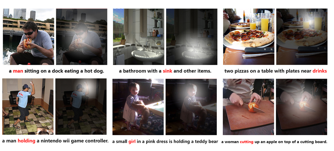
Figure 3: An example from our method generated result.

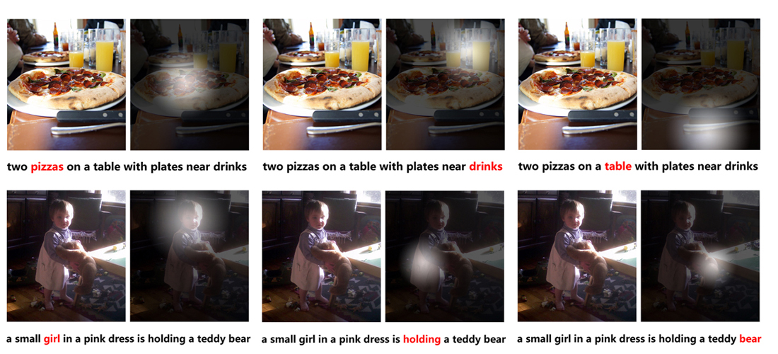
Figure 4: An example procedure from our method generated result.

5 Conclusion

This paper introduced a deep recurrent attention based approach, Recurrent Image Caption(RIC) model, that gives state of the art performance on three benchmark datasets using the BLEU and METEOR metric. The RIC model which is recurrent model consists of a encoder that sequential and gradually select finer input for the decoder and a decoder that is aimed to either directly maximize caption generation likelihood or maximize a variational lower bound. When working like the previous, our method is similar to that of [54] but a key difference is that our encoder is updated by decoder instead of simply depend on the input features, means that it can capture more fine details about images to generate more accurate captions, as shown in our experiment results. While when working like the later one, our method becomes a deep variational autoencoder in which the autoencoder try to reconstruct input image in the recurrent process and the process guided caption generation In this view, our work is related to [46] but a key difference is that in our encoder part, latent code is generated by conditioning on both image and sentence instead of simply use images to encode. In experiment we show that the above two kinds of recurrent model achieves state-of-the-art performance on several benchmarks.

References

- [1] D. Bahdanau, K. Cho, and Y. Bengio. Neural machine translation by jointly learning to align and translate. arXiv preprint arXiv:1409.0473, 2014.
- [2] S. Banerjee and A. Lavie. Meteor: An automatic metric for mt evaluation with improved correlation with human judgments. In Proceedings of the acl workshop on intrinsic and extrinsic evaluation measures for machine translation and/or summarization, volume 29, pages 65–72, 2005.
- [3] Y. Bin, Y. Yang, F. Shen, X. Xu, and H. T. Shen. Bidirectional long-short term memory for video description. In Proceedings of the 2016 ACM on Multimedia Conference, pages 436–440. ACM, 2016.
- [4] X. Chen, H. Fang, T.-Y. Lin, R. Vedantam, S. Gupta, P. Dollár, and C. L. Zitnick. Microsoft coco captions: Data collection and evaluation server. arXiv preprint arXiv:1504.00325, 2015.
- [5] X. Chen and C. Lawrence Zitnick. Mind’s eye: A recurrent visual representation for image caption generation. In Proceedings of the IEEE Conference on Computer Vision and Pattern Recognition, pages 2422–2431, 2015.
- [6] X. Chen and C. L. Zitnick. Learning a recurrent visual representation for image caption generation. arXiv preprint arXiv:1411.5654, 2014.
- [7] K. Cho, B. Van Merriënboer, C. Gulcehre, D. Bahdanau, F. Bougares, H. Schwenk, and Y. Bengio. Learning phrase representations using rnn encoder-decoder for statistical machine translation. arXiv preprint arXiv:1406.1078, 2014.
- [8] J. Dai, Y. Li, K. He, and J. Sun. R-fcn: Object detection via region-based fully convolutional networks. arXiv preprint arXiv:1605.06409, 2016.
- [9] L. Dinh, D. Krueger, and Y. Bengio. Nice: Non-linear independent components estimation. arXiv preprint arXiv:1410.8516, 2014.
- [10] L. Dinh, J. Sohl-Dickstein, and S. Bengio. Density estimation using real nvp. arXiv preprint arXiv:1605.08803, 2016.
- [11] J. Donahue, L. Anne Hendricks, S. Guadarrama, M. Rohrbach, S. Venugopalan, K. Saenko, and T. Darrell. Long-term recurrent convolutional networks for visual recognition and description. In Proceedings of the IEEE Conference on Computer Vision and Pattern Recognition, pages 2625–2634, 2015.
- [12] D. Elliott and F. Keller. Image description using visual dependency representations. In EMNLP, volume 13, pages 1292–1302, 2013.
- [13] H. Fang, S. Gupta, F. Iandola, R. K. Srivastava, L. Deng, P. Dollár, J. Gao, X. He, M. Mitchell, J. C. Platt, et al. From captions to visual concepts and back. In Proceedings of the IEEE Conference on Computer Vision and Pattern Recognition, pages 1473–1482, 2015.
- [14] A. Farhadi, M. Hejrati, M. A. Sadeghi, P. Young, C. Rashtchian, J. Hockenmaier, and D. Forsyth. Every picture tells a story: Generating sentences from images. In European Conference on Computer Vision, pages 15–29, 2010.
- [15] R. Frigola, Y. Chen, and C. Rasmussen. Variational gaussian process state-space models. In Advances in Neural Information Processing Systems, pages 3680–3688, 2014.
- [16] F. A. Gers, J. Schmidhuber, and F. Cummins. Learning to forget: Continual prediction with lstm. Neural computation, 12(10):2451–2471, 2000.
- [17] A. Graves. Generating sequences with recurrent neural networks. arXiv preprint arXiv:1308.0850, 2013.
- [18] A. Graves, G. Wayne, and I. Danihelka. Neural turing machines. arXiv preprint arXiv:1410.5401, 2014.
- [19] K. Gregor, I. Danihelka, A. Graves, D. J. Rezende, and D. Wierstra. Draw: A recurrent neural network for image generation. arXiv preprint arXiv:1502.04623, 2015.
- [20] K. He, X. Zhang, S. Ren, and J. Sun. Deep residual learning for image recognition. arXiv preprint arXiv:1512.03385, 2015.
- [21] S. Hochreiter and J. Schmidhuber. Long short-term memory. Neural computation, 9(8):1735–1780, 1997.
- [22] M. Hodosh, P. Young, and J. Hockenmaier. Framing image description as a ranking task: Data, models and evaluation metrics. Journal of Artificial Intelligence Research, 47:853–899, 2013.
- [23] R. Hong, Y. Yang, M. Wang, and X.-S. Hua. Learning visual semantic relationships for efficient visual retrieval. IEEE Transactions on Big Data, 1(4):152–161, 2015.
- [24] M. Jaderberg, K. Simonyan, A. Zisserman, et al. Spatial transformer networks. In Advances in Neural Information Processing Systems, pages 2017–2025, 2015.
- [25] A. Karpathy and L. Fei-Fei. Deep visual-semantic alignments for generating image descriptions. In Proceedings of the IEEE Conference on Computer Vision and Pattern Recognition, pages 3128–3137, 2015.
- [26] A. Karpathy, A. Joulin, and F. F. F. Li. Deep fragment embeddings for bidirectional image sentence mapping. In Advances in neural information processing systems, pages 1889–1897, 2014.
- [27] D. Kingma and J. Ba. Adam: A method for stochastic optimization. arXiv preprint arXiv:1412.6980, 2014.
- [28] R. Kiros, R. Salakhutdinov, and R. S. Zemel. Multimodal neural language models. In ICML, volume 14, pages 595–603, 2014.
- [29] R. Kiros, R. Salakhutdinov, and R. S. Zemel. Unifying visual-semantic embeddings with multimodal neural language models. arXiv preprint arXiv:1411.2539, 2014.
- [30] A. Krizhevsky, I. Sutskever, and G. E. Hinton. Imagenet classification with deep convolutional neural networks. In Advances in neural information processing systems, pages 1097–1105, 2012.
- [31] G. Kulkarni, V. Premraj, S. Dhar, S. Li, Y. Choi, A. C. Berg, and T. L. Berg. Baby talk: Understanding and generating image descriptions. In Proceedings of the 24th CVPR. Citeseer, 2011.
- [32] G. Kulkarni, V. Premraj, V. Ordonez, S. Dhar, S. Li, Y. Choi, A. C. Berg, and T. L. Berg. Babytalk: Understanding and generating simple image descriptions. IEEE Transactions on Pattern Analysis and Machine Intelligence, 35(12):2891–2903, 2013.
- [33] P. Kuznetsova, V. Ordonez, A. C. Berg, T. L. Berg, and Y. Choi. Collective generation of natural image descriptions. In Proceedings of the 50th Annual Meeting of the Association for Computational Linguistics: Long Papers-Volume 1, pages 359–368. Association for Computational Linguistics, 2012.
- [34] H. Larochelle and I. Murray. The neural autoregressive distribution estimator. In AISTATS, volume 1, page 2, 2011.
- [35] S. Li, G. Kulkarni, T. L. Berg, A. C. Berg, and Y. Choi. Composing simple image descriptions using web-scale n-grams. In Proceedings of the Fifteenth Conference on Computational Natural Language Learning, pages 220–228. Association for Computational Linguistics, 2011.
- [36] M. Liang and X. Hu. Recurrent convolutional neural network for object recognition. In Proceedings of the IEEE Conference on Computer Vision and Pattern Recognition, pages 3367–3375, 2015.
- [37] T.-Y. Lin, M. Maire, S. Belongie, J. Hays, P. Perona, D. Ramanan, P. Dollár, and C. L. Zitnick. Microsoft coco: Common objects in context. In European Conference on Computer Vision, pages 740–755. Springer, 2014.
- [38] E. Mansimov, E. Parisotto, J. L. Ba, and R. Salakhutdinov. Generating images from captions with attention. arXiv preprint arXiv:1511.02793, 2015.
- [39] J. Mao, X. Wei, Y. Yang, J. Wang, Z. Huang, and A. L. Yuille. Learning like a child: Fast novel visual concept learning from sentence descriptions of images. In Proceedings of the IEEE International Conference on Computer Vision, pages 2533–2541, 2015.
- [40] J. Mao, W. Xu, Y. Yang, J. Wang, Z. Huang, and A. Yuille. Deep captioning with multimodal recurrent neural networks (m-rnn). arXiv preprint arXiv:1412.6632, 2014.
- [41] J. Mao, W. Xu, Y. Yang, J. Wang, and A. L. Yuille. Explain images with multimodal recurrent neural networks. arXiv preprint arXiv:1410.1090, 2014.
- [42] M. Mathieu. Masked autoencoder for distribution estimation. 2015.
- [43] T. Mikolov, M. Karafiát, L. Burget, J. Cernockỳ, and S. Khudanpur. Recurrent neural network based language model. In Interspeech, volume 2, page 3, 2010.
- [44] V. Mnih, N. Heess, A. Graves, et al. Recurrent models of visual attention. In Advances in Neural Information Processing Systems, pages 2204–2212, 2014.
- [45] K. Papineni, S. Roukos, T. Ward, and W.-J. Zhu. Bleu: a method for automatic evaluation of machine translation. In Proceedings of the 40th annual meeting on association for computational linguistics, pages 311–318. Association for Computational Linguistics, 2002.
- [46] Y. Pu, Z. Gan, R. Henao, X. Yuan, C. Li, A. Stevens, and L. Carin. Variational autoencoder for deep learning of images, labels and captions. arXiv preprint arXiv:1609.08976, 2016.
- [47] C. Rashtchian, P. Young, M. Hodosh, and J. Hockenmaier. Collecting image annotations using amazon’s mechanical turk. In Proceedings of the NAACL HLT 2010 Workshop on Creating Speech and Language Data with Amazon’s Mechanical Turk, pages 139–147. Association for Computational Linguistics, 2010.
- [48] K. Simonyan and A. Zisserman. Very deep convolutional networks for large-scale image recognition. arXiv preprint arXiv:1409.1556, 2014.
- [49] I. Sutskever, O. Vinyals, and Q. V. Le. Sequence to sequence learning with neural networks. In Advances in neural information processing systems, pages 3104–3112, 2014.
- [50] C. Szegedy, W. Liu, Y. Jia, P. Sermanet, S. Reed, D. Anguelov, D. Erhan, V. Vanhoucke, and A. Rabinovich. Going deeper with convolutions. In Proceedings of the IEEE Conference on Computer Vision and Pattern Recognition, pages 1–9, 2015.
- [51] A. van den Oord, N. Kalchbrenner, and K. Kavukcuoglu. Pixel recurrent neural networks. arXiv preprint arXiv:1601.06759, 2016.
- [52] O. Vinyals, A. Toshev, S. Bengio, and D. Erhan. Show and tell: A neural image caption generator. In Proceedings of the IEEE Conference on Computer Vision and Pattern Recognition, pages 3156–3164, 2015.
- [53] Q. Wu, C. Shen, L. Liu, A. Dick, and A. v. d. Hengel. What value do explicit high level concepts have in vision to language problems? arXiv preprint arXiv:1506.01144, 2015.
- [54] K. Xu, J. Ba, R. Kiros, K. Cho, A. Courville, R. Salakhutdinov, R. S. Zemel, and Y. Bengio. Show, attend and tell: Neural image caption generation with visual attention. arXiv preprint arXiv:1502.03044, 2(3):5, 2015.
- [55] Y. Yang, C. L. Teo, H. Daumé III, and Y. Aloimonos. Corpus-guided sentence generation of natural images. In Proceedings of the Conference on Empirical Methods in Natural Language Processing, pages 444–454. Association for Computational Linguistics, 2011.
- [56] Y. Yang, Z.-J. Zha, Y. Gao, X. Zhu, and T.-S. Chua. Exploiting web images for semantic video indexing via robust sample-specific loss. IEEE Transactions on Multimedia, 16(6):1677–1689, 2014.
- [57] Y. Yang, H. Zhang, M. Zhang, F. Shen, and X. Li. Visual coding in a semantic hierarchy. In Proceedings of the 23rd ACM international conference on Multimedia, pages 59–68. ACM, 2015.
- [58] Q. You, H. Jin, Z. Wang, C. Fang, and J. Luo. Image captioning with semantic attention. arXiv preprint arXiv:1603.03925, 2016.
- [59] P. Young, A. Lai, M. Hodosh, and J. Hockenmaier. From image descriptions to visual denotations: New similarity metrics for semantic inference over event descriptions. Transactions of the Association for Computational Linguistics, 2:67–78, 2014.
- [60] W. Zaremba, I. Sutskever, and O. Vinyals. Recurrent neural network regularization. arXiv preprint arXiv:1409.2329, 2014.
- [61] H. Zhang, Y. Yang, H. Luan, S. Yang, and T.-S. Chua. Start from scratch: Towards automatically identifying, modeling, and naming visual attributes. In Proceedings of the 22nd ACM international conference on Multimedia, pages 187–196. ACM, 2014.
- [62] B. Zhou, A. Khosla, A. Lapedriza, A. Oliva, and A. Torralba. Learning deep features for discriminative localization. arXiv preprint arXiv:1512.04150, 2015.