Optimal polynomial meshes and Caratheodory-Tchakaloff submeshes
on the sphere

Abstract

Using the notion of Dubiner distance, we give an elementary proof of the fact that good covering point configurations on the 2-sphere are optimal polynomial meshes. From these we extract Caratheodory-Tchakaloff (CATCH) submeshes for compressed Least Squares fitting.

2010 AMS subject classification: 41A10, 65D32. Keywords: optimal polynomial meshes, Dubiner distance, sphere, good covering point configurations, Caratheodory-Tchakaloff subsampling, compressed Least Squares.

1 Dubiner distance and polynomial meshes

In this note we focus on two notions that have played a relevant role in the theory of multivariate polynomial approximation during the last 20 years: the notion of polynomial mesh and the notion of Dubiner distance in a compact set or manifold $K\subset\mathbb{R}^{d}$. Moreover, we connect the theory of polynomial meshes with the recent method of Caratheodory-Tchakaloff (CATCH) subsampling, working in particular on the sphere $S^{2}$.

In what follows we denote by $\mathbb{P}^{d}_{n}(K)$ the subspace of $d$-variate polynomials of total degree not exceeding $n$ restricted to $K$, and by $N=N_{n}(K)=\mbox{dim}(\mathbb{P}^{d}_{n}(K))$ its dimension. For example we have that $N={n+3\choose 3}=(n+1)(n+2)(n+3)/6$ for the ball in $\mathbb{R}^{3}$ and $N=(n+1)^{2}$ for the sphere $S^{2}$.

We briefly recall that a polynomial mesh on $K$ is a sequence of finite norming subsets $\mathcal{A}_{n}\subset K$ such that the following polynomial inequality holds

$$\|p\|_{L^{\infty}(K)}\leq C\,\|p\|_{\ell^{\infty}(\mathcal{A}_{n})}\;,\;\forall p\in\mathbb{P}_{n}^{d}(K)\;,$$ (1)

where $M_{n}=\mbox{card}(\mathcal{A}_{n})=\mathcal{O}(N^{\beta})$, $\beta\geq 1$. Indeed, since $\mathcal{A}_{n}$ is automatically $\mathbb{P}_{n}^{d}(K)$-determining (i.e., polynomials vanishing there vanish everywhere on $K$), then $M_{n}\geq N=\mbox{dim}(\mathbb{P}_{n}^{d}(K))=\mbox{dim}(\mathbb{P}_{n}^{d}(\mathcal{A}_{n}))$. Such a mesh is termed optimal when $\beta=1$.

In the case where $C$ is substituted by a sequence $C_{n}$ that increases subexponentially,

$$\|p\|_{L^{\infty}(K)}\leq C_{n}\,\|p\|_{\ell^{\infty}(\mathcal{A}_{n})}\;,\;\forall p\in\mathbb{P}_{n}^{d}(K)\;,$$ (2)

in particular when $C_{n}=\mathcal{O}(n^{s})$, $s\geq 0$, we speak of a weakly admissible polynomial mesh. All these notions can be given for $K\subset\mathbb{C}^{d}$ but we restrict here to the real case. The notion of polynomial mesh was introduced in the seminal paper [11] and then used from both the theoretical and the computational point of view, cf. e.g. [1, 4, 6, 10, 17, 24] and the references therein.

Polynomial meshes have indeed interesting computational features, e.g. they

• are affinely invariant and are stable under small perturbations [22]

• can be extended by algebraic transforms, finite union and product [6, 11]

• contain computable near optimal interpolation sets [4, 5]

• are near optimal for uniform Least Squares (LS) approximation (cf. [11, Thm. 1]), namely

  $$\Lambda(\mathcal{A}_{n})=\|\mathcal{L}_{\mathcal{A}_{n}}\|=\sup_{f\in C(K),f\neq 0}\frac{\|\mathcal{L}_{\mathcal{A}_{n}}^{w}f\|_{L^{\infty}(K)}}{\|f\|_{L^{\infty}(K)}}\leq C\,\sqrt{M_{n}}\;,$$ (3)

  where $\mathcal{L}_{\mathcal{A}_{n}}$ is the $\ell^{2}(\mathcal{A}_{n})$-orthogonal projection operator $C(K)\to\mathbb{P}_{n}^{d}(K)$ (the discrete LS operator at $\mathcal{A}_{n}$), from which easily follows

  $$\|f-\mathcal{L}_{\mathcal{A}_{n}}f\|_{L^{\infty}(K)}\leq\left(1+C\,\sqrt{M_{n}}\right)\,\min_{p\in\mathbb{P}_{n}^{d}(K)}\|f-p\|_{L^{\infty}(K)}\;.$$ (4)

We turn now to the notion of Dubiner distance in a compact set or manifold. Such a distance is defined as

$$\mbox{dist}_{D}(x,y)=\sup_{deg(p)\geq 1}\left\{\frac{1}{deg(p)}\,|\cos^{-1}(p(x))-\cos^{-1}(p(y))|\right\}\;,$$ (5)

where the sup is taken over the polynomials $p\in\mathbb{P}_{n}^{d}(K)$ such that $\|p\|_{L^{\infty}(K)}\leq 1$.

Introduced by M. Dubiner in the seminal paper [12], it belongs to a family of three distances (the other two are the Markov distance and the Baran distance) that play an important role in multivariate polynomial approximation and have deep connections with multivariate polynomial inequalities. We refer the readers, e.g., to [7, 8, 9] and to the references therein for relevant properties and results.

As far as we know, until now the Dubiner distance is known analytically only in very few instances: the interval (where it coincides with the usual distance $|\cos^{-1}(x)-\cos^{-1}(y)|$), the cube, the simplex, the ball, and the sphere. All these cases are treated in [7]. In particular, it can be proved via the classical van der Corput-Schaake inequality that on the sphere it coincides with the usual geodesic distance, namely

$$\mbox{dist}_{D}(x,y)=\gamma(x,y)=\cos^{-1}(\langle x,y\rangle)\;,\;\;\forall x,y\in S^{2}\;,$$ (6)

where $\langle x,y\rangle$ denotes the Euclidean scalar product in $\mathbb{R}^{3}$.

A simple connection of the Dubiner distance with the theory of polynomial meshes is given by the following:

Proposition 1

Let $\mathcal{A}_{n}$ be a compact subset of a compact set or manifold $K\subset\mathbb{R}^{d}$ whose covering radius with respect to the Dubiner distance does not exceed $\theta/n$, where $\theta\in(0,1)$ and $n\geq 1$, i.e.

$$\forall x\in K\;\exists y\in\mathcal{A}_{n}:\;\mbox{dist}_{D}(x,y)\leq\frac{\theta}{n}\;.$$ (7)

Then, the following inequality holds

$$\|p\|_{L^{\infty}(K)}\leq\frac{1}{1-\theta}\,\|p\|_{L^{\infty}(\mathcal{A}_{n})}\;,\;\;\forall p\in\mathbb{P}_{n}^{d}(K)\;.$$ (8)

In view of (7), the proof of Proposition 1 is an immediate consequence of the elementary inequality

$$|p(x)|\leq|p(y)|+|p(x)-p(y)|\leq|p(y)|+n\,\mbox{dist}_{D}(x,y)\,\|p\|_{L^{\infty}(K)}\;.$$ (9)

Observe, in particular, that $\mathcal{A}_{n}$ need not be discrete. In the case where (7) is satisfied by a sequence of finite subsets with $\mbox{card}(\mathcal{A}_{n})=\mathcal{O}(N^{\beta})$, $\beta\geq 1$, then these subsets clearly form a polynomial mesh like (1) for $K$, with $C=1/(1-\theta)$.

Let us now focus on the case of the sphere, $K=S^{2}$. We recall that a sequence of finite point configurations $X_{M}\subset S^{2}$, with cardinality $M\geq 2$, is termed a “good covering” of the sphere if its covering radius

$$\eta(X_{M})=\max_{x\in S^{2}}\min_{y\in X_{M}}|x-y|$$ (10)

satisfies the inequality

$$\eta(X_{M})\leq\frac{\alpha}{\sqrt{M}}\;,$$ (11)

for some $\alpha>0$ (cf., e.g., the survey paper [14]). It is then easy to prove the following result (that can be obtained also via a tangential Markov inequality on the sphere with exponent 1, cf. [15, 16]):

Proposition 2

Let $\{X_{M}\}$, $M\geq 1$, be a good covering of $S^{2}$. Then for every fixed $\theta\in(0,1)$ the sequence $\mathcal{A}_{n}=X_{M_{n}}$, with

$$M_{n}=\lceil\sigma_{n}^{2}n^{2}\rceil\;,\;\;\sigma_{n}=\frac{2\pi\alpha}{\theta(2\pi-\theta/n)}\sim\frac{\alpha}{\theta}\;,\;\;n\to\infty\;.$$ (12)

is an optimal polynomial mesh of $S^{2}$ with $C=1/(1-\theta)$.

Proof. By (10)-(11) and simple geometric considerations, for every $x\in S^{2}$ there exists $y\in X_{M}$ such that we have the estimate

$$\gamma(x,y)=2\sin^{-1}\left(\frac{|x-y|}{2}\right)\leq 2\sin^{-1}\left(\frac{\alpha}{2\sqrt{M}}\right)$$

(provided that $\alpha/(2\sqrt{M})\leq 1$ that is $\sqrt{M}\geq\alpha/2$), where $\gamma$ is the geodesic distance, i.e., the Dubiner distance. By Proposition 1, in order to determine $M_{n}$ it is the sufficient to fulfill the inequality

$$2\sin^{-1}\left(\frac{\alpha}{2\sqrt{M}}\right)\leq\frac{\theta}{n}$$

or equivalently

$$\frac{\alpha}{2\sqrt{M}}\leq\sin\left(\frac{\theta}{2n}\right)\;.$$ (13)

By the trigonometric inequality $\sin(t)\geq t(1-t/\pi)$, valid for $0\leq t\leq\pi$, we get

$$\sin\left(\frac{\theta}{2n}\right)\geq\frac{\theta}{2n}\,\left(1-\frac{\theta}{2\pi n}\right)\;,$$

and thus (13) is satisfied if

$$\frac{\alpha}{2\sqrt{M}}\leq\frac{\theta}{2n}\,\left(1-\frac{\theta}{2\pi n}\right)\;,$$

i.e. for $M\geq\sigma_{n}^{2}n^{2}$. $\;\;\;\;\;\square$

Among good covering configurations of $S^{2}$, an important role is played by the so-called “quasi-uniform” ones, that are those configurations with bounded ratio between the covering radius and the point separation (mesh ratio). Indeed, quasi-uniform configurations provide discretizations of the sphere that keep a low information redundancy. In [14] several quasi-uniform configurations are listed and their properties discussed. An interesting instance is the zonal equal area configurations (generated by zonal equal area partitions of the sphere), that turn out to be both, quasi-uniform and equidistributed in the sense of the surface area measure. In particular, they are theoretically good covering with $\alpha=3.5$ (but the numerical experiments suggest $\alpha=2.5$, cf. [18, 20]), and can be efficiently computed by the Matlab toolbox [19]. For example, taking $\theta=1/2$ by Proposition 2 we have the following quantitative result:

Corollary 1

The zonal equal area configurations with $M_{n}=\left\lceil 49\left(n-\frac{1}{4\pi}\right)^{2}\right\rceil$ points are an optimal polynomial mesh of the sphere with $C=2$.

The situation above is typical: polynomial meshes, even optimal ones, have often a large cardinality (though optimal as order of growth in $n$), which means large samples in the applications, for example in polynomial Least Squares. To this respect, it is useful to seek weakly admissible meshes with lower cardinality. This is exactly what we are going to do in the next Section, by the method of Caratheodory-Tchakaloff subsampling.

To conclude this Section, we observe that Proposition 1 can be used to generate optimal polynomial meshes in other cases where the Dubiner distance is explicitly known. For example, in the square $K=[-1,1]^{2}$

$$\mbox{dist}_{D}(x,y)=\max\left\{|\cos^{-1}(x_{1})-\cos^{-1}(x_{2})|,|\cos^{-1}(y_{1})-\cos^{-1}(y_{2})|\right\}\;.$$ (14)

We can then construct optimal polynomial meshes in $[-1,1]^{2}$ by the so-called Padua points. We recall that the Padua points of degree $k$ for the square $[-1,1]^{2}$ are given by the union of two Chebyshev-Lobatto subgrids

$$\mathcal{P}_{k}=\mathcal{C}_{k+1}^{even}\times\mathcal{C}_{k+2}^{odd}\cup\mathcal{C}_{k+1}^{odd}\times\mathcal{C}_{k+2}^{even}\;,$$ (15)

where $\mathcal{C}_{s+1}=\{\cos(j\pi/s)\,,\,\,0\leq j\leq s\}$, and the supscripts mean that only even or odd indexes are considered. They are a near-optimal point set for polynomial interpolation of total degree $k$, with a Lebesgue constant increasing as log square of the degree; cf., e.g., [3]. Extending a similar result for univariate Chebyshev-like points, we can prove the following

Proposition 3

The Padua points $\mathcal{P}_{\nu_{n}}$, $\nu_{n}=\left\lceil\frac{\pi n}{\theta}\right\rceil$, $0<\theta<1$ (cf. (15)), are an optimal polynomial mesh of the square with $C=(1-\theta)^{-1}$ and cardinality $M_{n}=(\nu_{n}+1)(\nu_{n}+2)/2$.

Proof. In view of (14), by simple geometric considerations we get easily that $\mbox{dist}_{D}(x,\mathcal{P}_{\nu_{n}})\leq\pi/\nu_{n}\leq\theta/n$, for every $x\in[-1,1]^{2}$. The result then follows immediately by Proposition 1. $\;\;\;\;\;\square$

We stress that the cardinality is asymptotically $\nu_{n}^{2}/2$, that is essentially half the cardinality obtainable by embedding the problem in the tensorial polynomial space $\mathbb{P}_{n}^{1}\otimes\mathbb{P}_{n}^{1}$, and using for example product Chebyshev points of degree $\nu_{n}$ (cf. [10, 30]).

1.1 Caratheodory-Tchakaloff (CATCH) submeshes

In order to reduce the cardinality of a polynomial mesh, a feature that is relevant in applications, we may try to relax the boundedness requirement for the ratio $\|p\|_{L^{\infty}(K)}/\|p\|_{\ell^{\infty}(\mathcal{A}_{n})}$, seeking a weakly admissible mesh contained in the original one, where the ratio is allowed to increase algebraically with respect to the polynomial space dimension $N$.

In principle, this can be done by computing Fekete points $\mathcal{F}_{n}\subset\mathcal{A}_{n}$. These are a subset of $\mathcal{A}_{n}$ that maximizes the Vandermonde determinant (not unique in general), so that the corresponding cardinal polynomials are bounded by 1 in $\ell^{\infty}(\mathcal{A}_{n})$, and by $C$ in $L^{\infty}(K)$. This entails that such discrete Fekete points are unisolvent and form a weakly admissible mesh of cardinality $N$, $C_{n}=CN$ being a bound on their Lebesgue constant [11]. Unfortunately, even the discrete Fekete points (as the continuous one) are difficult and costly to compute. In several papers, approximate Fekete points extracted from polynomial meshes have been computed by greedy algorithms based on standard numerical linear algebra routines; cf., e.g., [4, 5, 6]. These points work effectively for interpolation, and are asymptotically distributed as the continuous Fekete points, but no rigorous bound has been proved for their Lebesgue constant.

In the case of the sphere, the continuous Fekete (maximum determinant) points have been computed by a difficult numerical nonconvex optimization up to degrees in the hundreds, estimating also numerically the corresponding Lebesgue constants; cf. [32]. As it is well-known, the difficulties of polynomial interpolation on the sphere have led to the alternative approach of hyperinterpolation, cf. the seminal paper [26] and the numerous developments in the following 20 years.

In the present note, starting from optimal polynomial meshes of the sphere, we explore an alternative discrete approach, that can be considered a sort of fully discrete hyperinterpolation, namely the extraction of Caratheodory-Tchakaloff submeshes. These are computable by Linear or Quadratic Programming, and there are rigorous bounds for the corresponding constants $C_{n}$.

First, we recall a discrete version of the Tchakaloff theorem, a cornerstone of quadrature theory, whose proof is based on the Caratheodory theorem about finite dimensional conic combinations (cf., e.g., [2]). We focus here on total-degree polynomial spaces and we recall the proof to exhibit the connection with the Caratheodory theorem.

Theorem 1

Let $\mu$ be a multivariate discrete measure supported at a finite set $X=\{x_{i}\}\subset\mathbb{R}^{d}$, with correspondent positive weights (masses) $\boldsymbol{\lambda}=\{\lambda_{i}\}$, $i=1,\dots,M$.

Then, there exists a quadrature formula with nodes $T=\{t_{j}\}\subseteq X$ and positive weights $\boldsymbol{w}=\{w_{j}\}$, $1\leq j\leq m\leq N_{\nu}=\mbox{{\em dim\/}}(\mathbb{P}_{\nu}^{d}(X))$, such that

$$\int_{X}{p(x)\,d\mu}=\sum_{i=1}^{M}{\lambda_{i}\,p(x_{i})}=\sum_{j=1}^{m}{w_{j}\,p(t_{j})}\;,\;\;\forall p\in\mathbb{P}_{\nu}^{d}(X)\;.$$ (16)

Proof (cf., e.g., [21]). Let $\{p_{1},\dots,p_{N_{\nu}}\}$ be a basis of $\mathbb{P}_{\nu}^{d}(X)$, and $V=(v_{ij})=(p_{j}(x_{i}))$ the Vandermonde-like matrix of the basis computed at the support points. If $M>N_{\nu}$ (otherwise there is nothing to prove), existence of a positive quadrature formula for $\mu$ with cardinality not exceeding $N_{\nu}$ can be immediately translated into existence of a nonnegative solution with at most $N_{\nu}$ nonvanishing components to the underdetermined linear system

$$V^{t}\boldsymbol{u}=\boldsymbol{b}\;,\;\;\boldsymbol{u}\geq\boldsymbol{0}\;,$$ (17)

where

$$\boldsymbol{b}=V^{t}\boldsymbol{\lambda}=\left\{\int_{X}{p_{j}(x)\,d\mu}\right\}\;,\;\;1\leq j\leq N_{\nu}\;,$$ (18)

is the vector of $\mu$-moments of the basis $\{p_{j}\}$.

Existence then holds by the well-known Caratheodory theorem applied to the columns of $V^{t}$, which asserts that a conic (i.e., with positive coefficients) combination of any number of vectors in $\mathbb{R}^{N}$ can be rewritten as a conic combination of a linearly independent subset of at most $N_{\nu}$ of them.$\;\;\;\;\;\square$

We may term $T=\{t_{j}\}$ a set of Caratheodory-Tchakaloff (CATCH) quadrature points. We apply now the Tchakaloff theorem to the extraction of a weakly admissible submesh from a polynomial mesh.

Proposition 4

Let $\mathcal{A}_{n}\subset K$ be a polynomial mesh like (1) for $K$ with cardinality $M_{n}>N_{2n}=\mbox{dim}(\mathbb{P}_{2n}^{d}(K))$, let $\mu$ be the discrete measure with unit weights supported at $\mathcal{A}_{n}$, and let $T_{2n}=\{t_{j}\}$ be the $m\leq N_{2n}$ Caratheodory-Tchakaloff quadrature points for exactness degree $\nu=2n$ extracted from $\mathcal{A}_{n}$, with corresponding weights $\boldsymbol{w}=\{w_{j}\}$, $1\leq j\leq m$. Moreover, let $\mathcal{L}_{\mathcal{T}_{2n}}^{w}f\in\mathbb{P}_{n}^{d}(K)$ be the weighted discrete least squares polynomial on $T_{2n}$ for $f\in C(K)$.

Then $T_{2n}$ is a weakly-admissible polynomial mesh like (2) for $K$ with

$$C_{n}=C\sqrt{M_{n}}$$ (19)

(that we may term a Caratheodory-Tchakaloff submesh), and the following estimate holds for the corresponding weighted least squares approximation

$$\|f-\mathcal{L}_{T_{2n}}^{w}f\|_{L^{\infty}(K)}\leq\left(1+C_{n}\right)\,\min_{p\in\mathbb{P}_{n}^{d}(K)}\|f-p\|_{L^{\infty}(K)}\;.$$ (20)

Proof (cf., e.g., [31]). Since the Caratheodory-Tchakaloff quadrature is exact in $\mathbb{P}_{2n}^{d}(K)$, we get the basic $\ell^{2}$-identity

$$\|p\|^{2}_{\ell^{2}(\mathcal{A}_{n})}=\sum_{i=1}^{M_{n}}{p^{2}(x_{i})}=\sum_{j=1}^{m}{w_{j}\,p^{2}(t_{j})}=\|p\|^{2}_{\ell^{2}_{\boldsymbol{w}}(T_{2n})}\;,\;\;\forall p\in\mathbb{P}_{n}^{d}(K)\;.$$ (21)

Then we can write

$$\|p\|_{L^{\infty}(K)}\leq C\,\|p\|_{\ell^{\infty}(\mathcal{A}_{n})}\leq C\,\|p\|_{\ell^{2}(\mathcal{A}_{n})}=C\,\|p\|_{\ell^{2}_{\boldsymbol{w}}(T_{2n})}$$

$$\leq C\,\sqrt{\sum_{j=1}^{m}{w_{j}}}\;\;\|p\|_{\ell^{\infty}(T_{2n})}=C\,\sqrt{M_{n}}\,\|p\|_{\ell^{\infty}(T_{2n})}\;,$$ (22)

i.e., $T_{2n}$ is a weakly-admissible polynomial mesh for $K$ with $C_{n}=C\sqrt{M_{n}}$.

Concerning the weighted Least Squares polynomial approximation on $T_{2n}$, we recall that it is defined by

$$\|f-\mathcal{L}_{T_{2n}}^{w}f\|_{\ell^{2}_{\boldsymbol{w}}(T_{2n})}=\min_{p\in\mathbb{P}_{n}^{d}(K)}\|f-p\|_{\ell^{2}_{\boldsymbol{w}}(T_{2n})}$$ (23)

and that $\mathcal{L}_{T_{2n}}^{w}f$ is a $\ell^{2}_{\boldsymbol{w}}(T_{2n})$-orthogonal projection, i.e., $f-\mathcal{L}_{T_{2n}}^{w}f$ is $\ell^{2}_{\boldsymbol{w}}(T_{2n})$-orthogonal to $\mathbb{P}_{n}^{d}(K)$. Then,

$$\|\mathcal{L}_{T_{2n}}^{w}f\|_{L^{\infty}(K)}\leq C\,\|\mathcal{L}_{T_{2n}}^{w}f\|_{\ell^{\infty}(\mathcal{A}_{n})}\leq C\,\|\mathcal{L}_{T_{2n}}^{w}f\|_{\ell^{2}(\mathcal{A}_{n})}$$

$$=C\,\|\mathcal{L}_{T_{2n}}^{w}f\|_{\ell^{2}_{\boldsymbol{w}}(T_{2n})}\leq C\,\|f\|_{\ell^{2}_{\boldsymbol{w}}(T_{2n})}\leq C\,\sqrt{M_{n}}\,\|f\|_{L^{\infty}(K)}\;,$$

that is

$$\Lambda_{w}(T_{2n})=\|\mathcal{L}_{T_{2n}}^{w}\|=\sup_{f\in C(K),f\neq 0}\frac{\|\mathcal{L}_{T_{2n}}^{w}f\|_{L^{\infty}(K)}}{\|f\|_{L^{\infty}(K)}}\leq C_{n}=C\,\sqrt{M_{n}}\;,$$ (24)

from which (20) easily follows.$\;\;\;\;\;\square$

Observe that the error estimate (20) for weighted discrete Least Squares on the Caratheodory-Tchakaloff submesh, turns out to coincide with the natural error estimate (4) for unweighted Least Squares on the original polynomial mesh. In some sense, Caratheodory-Tchakaloff weighted Least Squares on the submesh catches all the relevant information from the polynomial mesh, as far as polynomial approximation in $\mathbb{P}_{n}^{d}(K)$ is concerned. We recall that the best uniform approximation error in $\mathbb{P}_{n}^{d}(K)$ can be estimated by the regularity of $f$, on compact sets $K$ admitting a Jackson-like theorem; cf., e.g., [23].

We can now apply the results above to optimal polynomial meshes on the sphere. Indeed, from Proposition 2 and 4 and Corollary 1 and 2 we get immediately the following

Corollary 2

Let $\mathcal{A}_{n}$ be a good covering optimal polynomial mesh as in Proposition 2, and let $T_{2n}$ be the extracted Caratheodory-Tchakaloff submesh (with corresponding weights).

Then, $T_{2n}$ is a weakly admissible mesh for the sphere with cardinality $N_{2n}=\mbox{{\em dim\/}}(\mathbb{P}^{3}_{2n}(S^{2}))=(2n+1)^{2}$, and (20) holds for the corresponding weighted Least Squares polynomial approximation $\mathcal{L}_{T_{2n}}^{w}f$ to $f\in C(S^{2})$, where

$$C_{n}=\frac{\sigma_{n}\,n}{1-\theta}\sim\frac{\alpha n}{\theta(1-\theta)}\;,\;\;n\to\infty\;.$$ (25)

In particular, for a Caratheodory-Tchakaloff submesh of the zonal equal area configurations of Corollary 1, we have

$$C_{n}=\frac{14n}{1-(4\pi n)^{-1}}\sim 14n\;,\;\;n\to\infty\;.$$ (26)

We observe that by ((3), (24) and (25) we get $\mathcal{O}(n)$ estimates for the least squares operator norms, whereas the best projection operators on $\mathbb{P}^{3}_{n}(S^{2})$ have a $\mathcal{O}(n^{1/2})$ norm; cf., e.g., [27]. On the other hand, (24) turns out to be an overestimate of the actual norm, as we shall see in the numerical examples.

1.2 Computational issues and numerical examples

In order to compute a sparse nonnegative solution to the underdermined system (17)-(18), that exists by Tchakaloff theorem (Theorem 1 above), there are a number of different approaches available. We focus here on the case of the sphere, where we use the classical spherical harmonics basis to define the Vandermonde-like matrix $V$.

A first approach resorts to Quadratic Programming, namely to the NonNegative Least Squares problem

$$\mbox{QP}:\;\;\;\left\{\begin{array}[]{ll}\min{\|V^{t}\boldsymbol{u}-\boldsymbol{b}\|_{2}}\\ \boldsymbol{u}\geq\boldsymbol{0}\end{array}\right.$$ (27)

which can be solved by the Lawson-Hanson active set method, which naturally seeks a sparse solution; cf. [21, 28] and the references therein. The nonzero components of $\boldsymbol{u}$ identify the weights $\boldsymbol{w}=\{w_{j}\}$ and the corresponding CATCH submesh $T_{2n}$.

A second approach is based on Linear Programming (cf. [21, 25, 29]), namely

$$\mbox{LP}:\;\;\;\left\{\begin{array}[]{ll}\min{\boldsymbol{c}^{t}\boldsymbol{u}}\\ V^{t}\boldsymbol{u}=\boldsymbol{b}\;,\;\;\boldsymbol{u}\geq\boldsymbol{0}\end{array}\right.$$ (28)

where the constraints identify a polytope (the feasible region), and the vector $\boldsymbol{c}$ is suitably chosen (cf. [21, 25]). Solving the problem by the classical Simplex Method, we get a vertex of the polytope, that is a nonnegative sparse solution to the underdetermined system.

A third combinatorial approach (Recursive Halving Forest), based on the SVD, is proposed in [29] and essentially applied to the reduction of Cartesian tensor cubature measures.

It is worth observing that sparsity cannot be ensured by the standard Compressive Sensing approach to underdetermined systems, such as the Basis Pursuit algorithm that minimizes $\|u\|_{1}$ (cf., e.g., [13]), since $\|u\|_{1}=\sqrt{M_{n}}$ is here constant by construction (being the quadrature formula applied to the constant polynomial $p\equiv 1$).

In our Matlab codes for Caratheodory-Tchakaloff Least Squares we have adopted both the QP approach (via an optimized version of the lsqnonneg function), and the LP approach (via the Simplex Method in the Matlab interface of the CPLEX package); cf. [21].

In Table 1, we report the numerical results corresponding to the extraction of CATCH submeshes from zonal equal area meshes of $S^{2}$, for a sequence of degrees. All the quantities are rounded to the first decimal digit. We have that the cardinality of the CATCH submeshes is $\mbox{dim}(\mathbb{P}_{2n}^{3}(S^{2}))=(2n+1)^{2}$, and that the Compression Ratio, $C_{ratio}=card(\mathcal{A}_{n})/card(T_{2n})$, increases, approaching the asymptotic value $49/4=12.25$, cf. Corollary 1. Since $\sum w_{j}=card(\mathcal{A}_{n})$, the average CATCH weight turns out to coincide with the Compression Ratio. Notice that the minimum of the CATCH weights computed by QP is much smaller than the minimum of the CATCH weights computed by LP.

Moreover, we see that the compressed least squares operator norms $\Lambda_{w}(T_{2n})$ are close to the norm $\Lambda(\mathcal{A}_{n})$ of the least squares operator on the starting mesh, with a slightly better behavior of CATCH submeshes extracted by QP with respect to those extracted by LP. On the other hand, all the norms are much lower than the theoretical overestimate $C_{n}\sim 14n$ in Corollary 2, having substantially a $\mathcal{O}(n^{1/2})$ increase (at least in the considered degree range).

In Table 2, we report the reconstruction errors by Least Squares (in the $L^{\infty}(S^{2})$-norm, numerically evaluated on a fine control grid), for three test functions with different degree of regularity

$$f_{1}(x_{1},x_{2},x_{3})=(x_{1}+x_{2}+x_{3})^{15}\;,\;\;f_{2}(x_{1},x_{2},x_{3})=\exp(x_{1}+x_{2}+x_{3})/10\;,\;\;$$

$$f_{3}(x_{1},x_{2},x_{3})=(|x_{1}|+|x_{2}|+|x_{3}|)/10\;,\;\;$$ (29)

namely a polynomial, a smooth function and a function with singular points on the sphere (the latter two taken from [32]).

Finally, in Figure 1 we display the CATCH submesh extracted by QP from a zonal equal area mesh for degree $n=5$.

Table 1: Cardinality of zonal equal area meshes $\mathcal{A}_{n}$ and of their CATCH submeshes $T_{2n}$, Compression Ratio, weight ratios, discrete least squares operator norms (the CATCH weights and submeshes have been obtained by (27) via lsqnonneg and by (28) via CPLEX).

deg $n$	2	5	8	11	14	17	20
$card(\mathcal{A}_{n})$	181	1187	3074	5844	9496	14029	19445
$card(T_{2n})$	25	121	289	529	841	1225	1681
$C_{ratio}$ ($=w_{avg}$)	$7.2$	$9.8$	$10.6$	$11.0$	$11.3$	$11.5$	$11.6$
QP: $w_{max}/w_{avg}$	2.2	2.6	2.5	2.5	2.6	2.4	2.6
LP: $w_{max}/w_{avg}$	2.1	3.1	2.8	3.1	3.1	3.0	3.0
QP: $w_{min}/w_{avg}$	2.1e-2	5.4e-4	7.6e-5	8.8e-6	2.4e-6	8.1e-6	2.6e-6
LP: $w_{min}/w_{avg}$	9.1e-2	4.3e-4	2.3e-3	6.2e-4	1.1e-3	2.4e-3	1.3e-3
$\Lambda(\mathcal{A}_{n})$	2.2	3.3	4.2	4.9	5.6	6.2	6.7
$1.5\,n^{1/2}$	2.1	3.4	4.2	5.0	5.6	6.2	6.7
QP: $\Lambda_{w}(T_{2n})$	2.5	3.7	4.6	5.4	6.0	6.5	7.1
LP: $\Lambda_{w}(T_{2n})$	2.6	4.2	5.6	6.6	7.4	7.5	8.4

Table 2: Absolute errors ($L^{\infty}(S^{2})$-norm) in the reconstruction of the three test functions (29) by unweighted Least Squares on zonal equal area meshes $\mathcal{A}_{n}$ and by weighted Least Squares on their CATCH submeshes $T_{2n}$.

	deg $n$	2	5	8	11	14	17	20
	LS	1.4e+5	4.1e+4	1.5e+4	5.3e+2	3.7e+1	8.4e-10	9.1e-10
$f_{1}$	CATCHQP	1.7e+5	4.8e+4	1.4e+4	5.1e+2	3.7e+1	8.4e-10	6.4e-10
	CATCHLP	2.0e+5	4.6e+4	1.6e+4	6.5e+2	4.3e+1	5.8e-10	6.7e-10
	LS	1.3e-1	1.6e-3	5.1e-6	5.9e-9	3.3e-12	5.6e-15	6.2e-15
$f_{2}$	CATCHQP	1.7e-1	1.7e-3	5.1e-6	6.0e-9	3.3e-12	2.8e-15	1.9e-15
	CATCHLP	1.3e-1	1.7e-3	4.5e-6	6.7e-9	3.3e-12	2.1e-15	2.6e-15
	LS	5.0e-1	3.2e-1	1.5e-1	1.4e-1	9.5e-2	9.2e-2	7.4e-2
$f_{3}$	CATCHQP	6.0e-1	3.4e-1	1.9e-1	1.6e-1	1.2e-1	9.7e-2	7.4e-2
	CATCHLP	6.0e-1	3.7e-1	1.9e-1	1.5e-1	1.3e-1	1.0e-1	1.1e-1

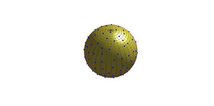
Figure 1: CATCH submesh (121 points, bullets) extracted by NNLS from a zonal equal area mesh (1187 points, dots) of the sphere for degree $n=5$.

References

- [1] T. Bloom, L. Bos, J.-P. Calvi and N. Levenberg, Polynomial interpolation and approximation in , Ann. Polon. Math. 106 (2012), 53–81.
- [2] J.M. Borwein and J.D. Vanderwerff, Convex functions: constructions, characterizations and counterexamples, Cambridge University Press, Cambridge, 2010.
- [3] L. Bos, M. Caliari, S. De Marchi, M. Vianello and Y. Xu, Bivariate Lagrange interpolation at the Padua points: the generating curve approach, J. Approx. Theory 143 (2006), 15–25.
- [4] L. Bos, J.-P. Calvi, N. Levenberg, A. Sommariva and M. Vianello, Geometric Weakly Admissible Meshes, Discrete Least Squares Approximation and Approximate Fekete Points, Math. Comp. 80 (2011), 1601–1621.
- [5] L. Bos, S. De Marchi, A. Sommariva and M. Vianello, Computing multivariate Fekete and Leja points by numerical linear algebra, SIAM J. Numer. Anal. 48 (2010), 1984–1999.
- [6] L. Bos, S. De Marchi, A. Sommariva and M. Vianello, Weakly Admissible Meshes and Discrete Extremal Sets, Numer. Math. Theory Methods Appl. 4 (2011), 1–12.
- [7] L. Bos, N. Levenberg and S. Waldron, Metrics associated to multivariate polynomial inequalities, Advances in Constructive Approximation, M. Neamtu and E. B. Saff eds., Nashboro Press, Nashville, 2004, 133–147.
- [8] L. Bos, N. Levenberg and S. Waldron, Pseudometrics, distances and multivariate polynomial inequalities J. Approx. Theory 153 (2008), 80–96.
- [9] L. Bos, N. Levenberg and S. Waldron, On the spacing of Fekete points for a sphere, ball or simplex, Indag. Math. 19 (2008), 163–176.
- [10] L. Bos and M. Vianello, Low cardinality admissible meshes on quadrangles, triangles and disks, Math. Inequal. Appl. 15 (2012), 229–235.
- [11] J.P. Calvi and N. Levenberg, Uniform approximation by discrete least squares polynomials, J. Approx. Theory 152 (2008), 82–100.
- [12] M. Dubiner, The theory of multidimensional polynomial approximation, J. Anal. Math. 67 (1995), 39–116.
- [13] S. Foucart and H. Rahut, A Mathematical Introduction to Compressive Sensing, Birkhäuser, 2013.
- [14] D.P. Hardin, T. Michaels and E.B. Saff, A Comparison of Popular Point Configurations on , Dolomites Res. Notes Approx. DRNA 9 (2016), 16–49.
- [15] K. Jetter, J. Stöckler and J.D. Ward, Norming sets and spherical cubature formulas, in: Advances in computational mathematics (Guangzhou, 1997), 237–244, Lecture Notes in Pure and Appl. Math. 202, Marcel-Dekker, New York, 1998.
- [16] K. Jetter, J. Stöckler and J.D. Ward, Error estimates for scattered data interpolation on spheres, Math. Comp. 68 (1999), 733–747.
- [17] A. Kroó, On optimal polynomial meshes, J. Approx. Theory 163 (2011), 1107–1124.
- [18] P. Leopardi, A partition of the unit sphere into regions of equal area and small diameter, Electron. Trans. on Numer. Anal. 25 (2006), 309–327.
- [19] P. Leopardi, Recursive Zonal Equal Area Sphere Partitioning Toolbox, http://eqsp.sourceforge.net.
- [20] P. Leopardi, Distributing points on the sphere: partitions, separation, quadrature and energy, Ph.D. Thesis, The University of New South Wales, April 2007.
- [21] F. Piazzon, A. Sommariva and M. Vianello, Caratheodory-Tchakaloff Least Squares (paper and codes), submitted to the pre-proceedings of SampTA 2017, online at: www.math.unipd.it/~marcov/publications.html.
- [22] F. Piazzon and M. Vianello, Small perturbations of polynomial meshes, Appl. Anal. 92 (2013), 1063–1073.
- [23] W. Pleśniak, Multivariate Jackson Inequality, J. Comput. Appl. Math. 233 (2009), 815–820.
- [24] W. Pleśniak, Nearly optimal meshes in subanalytic sets, Numer. Algorithms 60 (2012), 545–553.
- [25] E.K. Ryu and S.P. Boyd, Extensions of Gauss quadrature via linear programming, Found. Comput. Math. 15 (2015), 953–971.
- [26] I.H. Sloan, Interpolation and Hyperinterpolation over General Regions, J. Approx. Theory 83 (1995), 238–254.
- [27] I.H. Sloan and R.S. Womersley, Constructive polynomial approximation on the sphere. J. Approx. Theory 103 (2000), 91–118.
- [28] A. Sommariva and M. Vianello, Compression of multivariate discrete measures and applications, Numer. Funct. Anal. Optim. 36 (2015), 1198–1223.
- [29] M. Tchernychova, “Caratheodory” cubature measures, Ph.D. dissertation in Mathematics (supervisor: T. Lyons), University of Oxford, 2015.
- [30] M. Vianello, Norming meshes by Bernstein-like inequalities, Math. Inequal. Appl. 17 (2014), 929–936.
- [31] M. Vianello, Compressed sampling inequalities by Tchakaloff’s theorem, Math. Inequal. Appl. 19 (2016), 395–400.
- [32] R.S. Womersley and I.H. Sloan, How good can polynomial interpolation on the sphere be? Adv. Comput. Math. 14 (2001), 195–226.