Mg II Absorption at $2<z<7$ with Magellan/FIRE, III. Full Statistics of Absorption towards 100 High-Redshift QSOs

Abstract

We present statistics from a survey of intervening Mg ii absorption towards 100 quasars with emission redshifts between $z=3.55$ and $z=7.09$. Using infrared spectra from Magellan/FIRE, we detect 280 cosmological Mg ii absorbers, and confirm that the comoving line density of $W_{r}>0.3$ Å Mg ii absorbers does not evolve measurably between $z=0.25$ and $z=7$. This is consistent with our detection of seven Mg ii systems at $z>6$, redshifts not covered in prior searches. Restricting to systems with $W_{r}>1$Å, there is significant evidence for redshift evolution. These systems roughly double in density between $z=0$ and $z=2$-$3$, but decline by an order of magnitude from this peak by $z\sim 6$. This evolution mirrors that of the global star formation rate density, potentially reflecting a connection between star formation feedback and the strong Mg ii absorbers. We compared our results to the Illustris cosmological simulation at z=2-4 by assigning absorption to catalogued dark-matter halos and by direct extraction of spectra from the simulation volume. Reproducing our results using the former requires circumgalactic MgII envelopes within halos of progressively smaller mass at earlier times. This occurs naturally if we define the lower integration cutoff using SFR rather than mass. Spectra calculated directly from Illustris yield too few strong Mg ii absorbers. This may arise from unresolved phase space structure of circumgalactic gas, particularly from spatially unresolved turbulent or bulk motions. The presence of circumgalactic magnesium at $z>6$ suggests that enrichment of intra-halo gas may have begun before the presumed host galaxies’ stellar populations were mature and dynamically relaxed.

1. Introduction

For over 30 years (Bergeron, 1986; Bergeron & Boissé, 1991; Bahcall & Spitzer, 1969), the Mg ii doublet has been recognized as an absorption signature of enriched gas in the halos of luminous galaxies. While most Mg is singly ionized in the Galactic disk on account of the 0.56 Ryd ionization energy of Mg i, blind absorption surveys predominantly identify discrete Mg ii absorbers (e.g. above an equivalent width threshold of $W_{r}\sim 0.1-0.3$Å) in the more extended halos of distant galaxies at impact parameters of 10-100 kpc, or a few tenths of $R_{vir}$ (Chen et al., 2010; Zibetti et al., 2007; Bouché et al., 2007; Gauthier et al., 2010; Lovegrove & Simcoe, 2011; Churchill et al., 2000; Werk et al., 2013; Churchill et al., 2013). Gas at these impact parameters presents a larger cross section for chance absorption, yet retains pockets of sufficient density that H i can shield Mg ii ions against photons with their ionization energy of 1.1 Ryd.

The empirical association of galaxies with intra-halo Mg ii gas, together with the heavy element enrichment implied by Mg, invites the interpretation that Mg ii absorption arises in regions polluted by galactic winds. This is an attractive picture because simulations of galaxy formation require vigorous amounts of mechanical and thermal feedback to match galaxies’ stellar mass function and mass-metallicity relation (Vogelsberger et al., 2014a), and the halo is a convenient place to deposit baryons ejected from the disk during this process. Unfortunately these same simulations are not always well-suited to make detailed predictions of Mg ii properties of circum-galactic gas. In regions of the temperature-density plane where the Mg ii ionization fraction peaks, numerical codes often transition into sub-grid scalings for cooling and mass flow (Vogelsberger et al., 2014b).

Simple analytic calculations of the total circum-galactic mass and metal budget from observations of projected galaxy-QSO or QSO-QSO pairs derive very large masses (Tumlinson et al., 2011; Bordoloi et al., 2014; Stern et al., 2016; Prochaska et al., 2013), despite the fact that ionization models for individual optically thick absorbers consistently yield line-of-sight sizes measured in tens of physical parsecs (Charlton et al., 2003; Misawa et al., 2008; Lynch & Charlton, 2007; Simcoe et al., 2006; Stern et al., 2016). This is corroborated by observations of Mg ii absorption in lensed QSOs which show variations in low ionization absorption (Mg ii, Si ii, and C ii) on transverse scales ranging from 26$h^{-1}$ pc (Rauch et al., 1999) to 200-300 $h^{-1}$ pc (Rauch et al., 2002). These findings suggest that Mg ii absorbing gas is highly structured in halos even as observations of the high covering fraction show that it is widespread.

Further complicating the picture from simulations, the halo is expected to harbor accreting gas at similar densities, both on first infall from the IGM (Dekel et al., 2009; Kereš et al., 2005; Faucher-Giguère & Kereš, 2011; Fumagalli et al., 2014), and recycled from previous generations of star forming winds that remained bound to the dark matter halo (Oppenheimer et al., 2010; Ford et al., 2016).

Indeed, infalling Mg ii absorption has been seen directly in down-the-barrel spectra of selected nearby galaxies (Rubin et al., 2012), in contrast to the common outflowing/blueshifted Mg ii seen in stacks of galaxy spectra at similar redshift (Weiner et al., 2009). Apparently galaxy halos contain Mg ii gas from both inflowing and outflowing baryons in unknown proportion. Morphological analysis of absorber host galaxies lends tentative evidence to this hypothesis, since strong absorption is slightly more likely out of the disk plane, while weaker absorbers can align with the orientation of the disk (Bouché et al., 2007; Bordoloi et al., 2011; Kacprzak et al., 2011; Nielsen et al., 2015).

Models of accretion flows and galactic winds both exhibit redshift dependence, but Mg ii observations in optical spectrographs probe a maximum absoprtion redshift of $z\sim 2.5$. In Matejek & Simcoe (2012, hereafter Paper I), we presented initial results on an infrared survey for Mg ii absorbers at $2<z<5.5$, using the FIRE spectrograph on Magellan (Simcoe et al., 2013). Out of necessity, the IR sample is much smaller than optical Mg ii surveys, which include up to $\geq 30,000$ doublets (Nestor et al., 2005; Prochter et al., 2006; Lundgren et al., 2009; Quider et al., 2011; Seyffert et al., 2013; Zhu & Ménard, 2013; Chen et al., 2015; Raghunathan et al., 2016). Since Mg ii appears to trace both star-formation feedback (Bond et al., 2001; Weiner et al., 2009; Ménard et al., 2011; Zibetti et al., 2007; Bouché et al., 2007; Nestor et al., 2011; Martin et al., 2012; Kornei et al., 2012) and cool accretion (Steidel et al., 2002; Kereš et al., 2005; Rubin et al., 2010; López & Chen, 2012; Bouché et al., 2016), our aim was to extend redshift coverage past the peak in the star formation rate density, providing statistics on absorption during the buildup phase of stellar mass.

For robust statistics, our goal was to observe $\sim 100$ QSOs with FIRE and identify 100-200 absorbers. Paper I presented the first 46 sightlines, limited by observing time and weather. Here we update these results to include 54 additional sightlines for a total sample of 100 objects, constituting the full survey.

Paper I focused on bright QSOs to build up the sample; a consequence of this choice is that our statistics were best at $2<z<4$ because of the abundance of bright background sources. A key result of this early paper was evidence for evolution in the frequency of strong Mg ii absorbers ($W_{r}>1.0$Å), which peak in number density near $z\sim 2.5$ and then decline toward higher redshift. The significance of this result hinged on decreasing numbers of strong Mg ii in the highest redshift bins, which contained less survey pathlength because the highest redshift ($z>6$) background sources are rarer and fainter.

In the intervening time, new wide-area surveys with near-IR color information have yielded numerous examples of bright $z>5.5$ QSOs in the Southern Hemisphere and therefore accessible for FIRE observation (Bañados et al., 2016; Jiang et al., 2016; Venemans et al., 2015a, b; Willott et al., 2010; Venemans et al., 2013; Bañados et al., 2014). These sightlines are suitable for Mg ii absorption surveys and this paper employs a larger proportion of observing time on them, with a goal of improving statstics at $z>4$. By emphasizing these high-redshift targets we also obtain greater overlap with pioneering investigations cool absorbing gas at $z>6$ (Becker et al., 2006, 2011) that focused on low-ionization O i, C ii, and Si ii visible in high-resolution optical spectra. These authors speculate that cool absorbing gas populates the circum-galactic media of galaxies that are too faint to observe at present, but which are thought to be important for hydrogen reionization.

We employ largely the same analysis techniques as Paper I utilizing the new and larger Mg ii sample. In Sections 2 and 3 we describe the methods for data collection, continuum fitting, line finding, and tests for completness and sample contamination from false-positives. Section 4 presents updated results on the line density and evolution of Mg ii frequency and absorber equivalent width distributions. Section 5 discusses these results in the context of different models for Mg ii production. For comoving calculations we assume a cosmology derived from the the Planck 2016 results with $H_{0}=67.27,\Omega_{M}=0.3156,\Omega_{\Lambda}=1-\Omega_{\Lambda}$ throughout (Planck Collaboration et al., 2016a).

2. Data

This paper expands the original Mg ii survey of Paper I to 100 sightlines, adding 54 objects to our original sample of 46. This achieves our original goal of surveying $\sim 100$ QSOs, while focusing more heavily on quasars with high emission redshift. This approach carries a larger observational cost, but was motivated by the findings of Paper I—specifically, that the strongest Mg ii absorbers decline in frequency above $z\sim 3$ but weaker systems with $W_{r}=0.3-1.0$Å remain nearly constant in comoving number density. These results hinged on the highest redshift bins of the original sample, which had the shortest absorption path and therefore the highest uncertainty.

Our sightlines are drawn from a number of quasar surveys. The majority of the sample is drawn from the SDSS DR7 QSO catalog (Schneider et al., 2010) and dedicated high redshift SDSS searches (Jiang et al., 2016), but significant numbers are also derived from the BR and BRI catalogs which contain many Southern APM-selected quasars (Storrie-Lombardi et al., 1996). Many of the new $z>6$ sightlines observed for this paper are drawn from searches for $i$ and $z$ dropouts in the UKIDSS, PanStarrs, and VISTA/VIKING surveys (Mortlock et al., 2011; Venemans et al., 2015b, a; Bañados et al., 2016; Willott et al., 2010; Venemans et al., 2013; Bañados et al., 2014; Venemans, 2017; Mazzucchelli, 2017), which now have discovered a significant fraction of all known $z>5.5$ QSOs. Objects were selected for observation based on the QSO’s redshift and apparent magnitude. No consideration was given to the intrinsic properties of the background objects other than a screening to avoid broad absorption line (BAL) quasars, which contain extended intrinsic absorption that can be confused with intervening, cosmological lines.

All obervations were conducted with FIRE, which is a single object, prism cross-dispersed infrared spectrometer on the Magellan Baade telescope (Simcoe et al., 2013). We observed with a 0.6^′′ slit, yielding a spectral resolution of $R=6000$, or approximately 50 km s^-1, over the range 0.8 to 2.5 $\mu$m. A complete list of these QSOs may be found in Table 1. The spectra were reduced using the IDL FIREHOSE pipeline, which performs 2D sky subtraction using the algorthms outlined in Kelson (2003) and extracts an optimally weighted 1D spectrum. Telluric corrections and flux calibration are performed using concurrently observerd A0V standard stars, which are input to the xtellcor routine drawn from the spextool software library(Cushing et al., 2004; Vacca et al., 2003). The signal-to-noise ratios (SNRs) of the spectra vary substantially and are indicated in Table 1; these differences are accounted during the completeness corrections outlined in Section 3.

The lower redshift limit for our Mg ii absorption search is $z\approx 1.9$, set by the wavelength coverage of FIRE as in the original survey. The upper limit, fixed at 3000 km s^-1 below the emission redshifts of the QSOs, has been significatly increased. Whereas the maximum QSO emission redshift in original survey was $z=6.28$ (set by SDSS1030+0524), our sample now includes six QSOs with emission redshift $z>6.5$, including ULAS1120+0641 at $z=7.09$ (Fig. 1).

Despite having several objects with emisison redshifts $z_{em}>6$, the original survey had an absorption redshift limit of only $z_{abs}=5.4$ even though we observed several quasars at $z\gtrsim 6$. This reflects limitations from atmospheric absorption between the $H$ and $K$ bands, which cuts out Mg ii pathlength from $5.4<z<5.9$. Paper I included too few objects with coverage above $z=6$ to derive meaningful constraints on Mg ii in this epoch. For this paper, we have therefore dedicated the majority of our observing time to fainter QSOs at $z=6$ and above, thereby increasing our constraining power on the column density of Mg ii absorbers at these at earlier redshifts, rather than strictly maximizing the total number of QSOs observed. Our expanded sample has more than doubled the pathlength above $z=5.5$, and the median emission redshift has increased from $\langle z\rangle=4.27$ to $\langle z\rangle=4.63$.

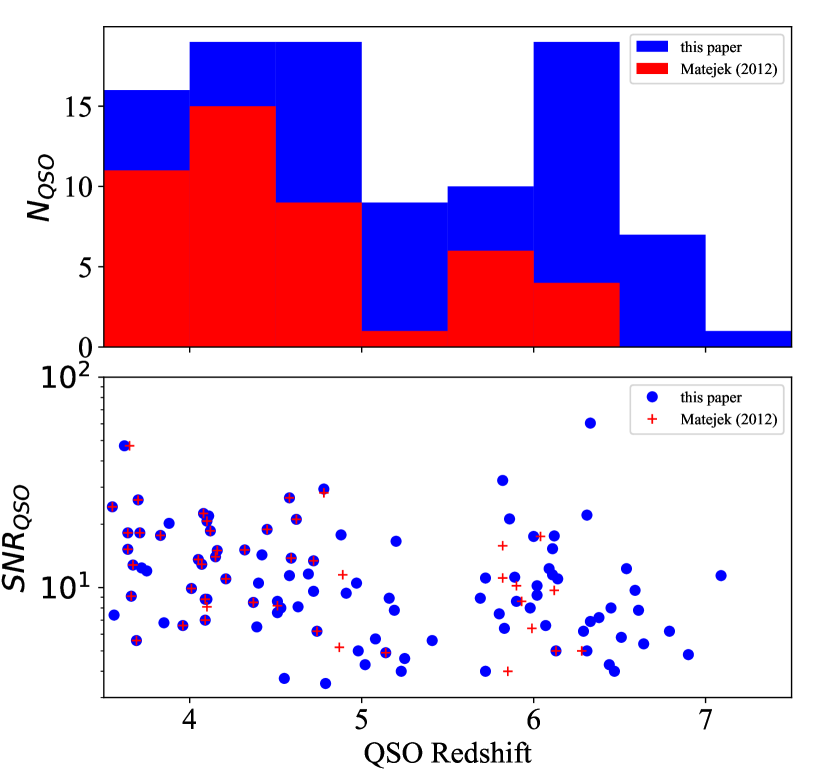
Figure 1.— (Top) A histogram of our quasar sample by emission redshift (blue) as compared to the original sample (red), in bins of $\Delta z=0.5$. The number of QSO’s studied beyond z = 5.5 has been doubled, and the median emission redshift has been increased from z = 4.27 to z = 4.63. (Bottom) A scatterplot showing the emission redshift and signal-to-noise ratios of our quasar spectra as compared to Matejek & Simcoe (2012).

Table 1FIRE Mg ii Survey Sightlines

Quasar	$z_{em}$	$\Delta z$	$t_{exp}$	Median SNR	RA	DEC
			(sec.)	(pixel-1)
Q0000-26	4.10	1.95-3.83	1226	20.7	00:03:22.9	-26:03:18.8
BR0004-6224	4.51	1.95-4.51	1764	7.6	00:06:51.6	-62:08:03.7
BR0016-3544	4.15	1.95-3.83	2409	14.0	00:18:37.9	-35:27:40.
SDSS J0040-0915	4.97	1.95-4.97	2409	10.5	00:40:54.65	-09:15:26.0
SDSS J0042-1020	3.88	1.95-3.83	4818	20.2	00:42:19.74	-10:20:09.5
SDSS J0054-0109	5.08	1.95-5.08	4501	5.7	00:54:21.43	-01:09:21.0
SDSS J0100+2802	6.33	2.19-6.33	18652	60.5	01:00:13.02	+28:02:25.84
SDSS 0106+0048	4.45	1.95-4.45	3635	18.9	01:06:19.2	+00:48:23.
VIK J0109-3047	6.79	2.39-6.79	28511	6.2	01:09:53.1	-30:47:26.3
SDSS J0113-0935	3.67	1.95-3.67	1944	12.8	01:13:51.96	-09:35:51.1
SDSS J0127-0045	4.08	1.95-3.83	3635	22.5	01:27:00.69	-00:45:59.2
SDSS J0140-0839	3.71	1.95-3.71	1226	18.2	01:40:49.18	-08:39:42.5
SDSS J0157-0106	3.56	1.95-3.56	1817	7.4	01:57:41.57	-01:06:29.6
PSO J029-29	5.99	2.04-5.98	4501	8.0	01:58:04.14	-29:05:19.25
ULAS J0203+0012	5.72	1.95-5.40	3635	4.0	02:03:32.38	+00:12:29.27
SDSS J0216-0921	3.72	1.95-3.72	1920	12.4	02:16:46.9	-09:21:07.0
SDSS J0231-0728	5.41	1.95-5.40	2409	5.6	02:31:37.6	-07:28:54.0
SDSS J0244-0816	4.07	1.95-3.83	1944	12.9	02:44:47.8	-08:16:06.0
VST-ATLAS J025-33	6.31	2.18-6.31	18926	22.1	01:40:55.56	-33:27:45.72
VIK J0305-3150	6.61	2.31-6.61	26400	7.8	03:05:16.916	-31:50:55.98
BR0305-4957	4.78	1.95-4.78	2409	29.4	03:07:22.9	-49:45:48.0
BR0322-2928	4.62	1.95-4.62	2409	21.1	03:24:44.3	-29:18:21.1
BR0331-1622	4.32	1.95-4.32	1944	15.1	03:34:13.4	-16:12:05.2
SDSS J0331-0741	4.74	1.95-4.74	2177	6.2	03:31:19.7	-07:41:43.1
SDSS J0332-0654	3.69	1.95-3.69	2409	5.6	03:32:23.5	-06:54:50.0
SDSS J0338+0021	5.02	1.95-5.02	1817	4.3	03:38:29.3	+00:21:56.5
SDSS J0344-0653	3.96	1.95-3.83	3022	6.6	03:44:02.85	-06:53:00.6
BR0353-3820	4.58	1.95-4.58	1200	26.7	03:55:04.9	-38:11:42.3
PSO J036+03	6.54	2.28-6.54	10240	12.3	02 26 01.88	+03 02 59.4
BR0418-5723	4.37	1.95-4.37	4200	8.5	04:19:50.9	-57:16:13.0
PSO J071-02	5.70	1.95-5.40	1817	6.9	04:45:48.18	-02:19:59.8
DES J0454-4448	6.09	2.08-6.09	19878	12.3	04:54:01.79	-44:48:31.1
PSO 065-26	6.14	2.10-6.14	7228	11.0	04:21:38.05	-26:57:15.6
PSO J071-02	5.69	1.95-5.40	3614	8.9	04:45:48.18	-02:19:59.8
SDSS J0759+1800	4.79	1.95-4.79	2409	3.5	07:59:07.57	+18:00:54.71
SDSS J0817+1351	4.39	1.95-4.39	2409	6.5	08:17:40.50	+13:51:35.0
SDSS J0818+0719	4.58	1.95-4.39	2409	11.4	08:18:06.9	+07:19:20.0
SDSS J0818+1722	6.02	2.00-5.40	9000	10.2	08:18:27.10	+17:22:51.79
SDSS J0824+1302	5.19	1.95-5.19	4818	7.8	08:24:54.02	+13:02:17.01
SDSS J0836+0054	5.81	1.96-5.40	33200	32.3	08:36:43.9	+00:54:53.3
SDSS J0842+1218	6.07	2.07-6.07	7228	6.6	15:58:50.99	-07:24:09.6
SDSS J0842+0637	3.66	1.95-3.66	2409	9.1	08:42:03.3	+06:37:52.0
SDSS J0902+0851	5.23	1.95-5.20	3001	4.0	09:02:45.76	+08:51:15.8
SDSS J0935+0022	3.75	1.96-5.40	1817	12.0	09:35:56.9	+00:22:55.0
SDSS J0949+0335	4.05	1.95-3.83	1817	13.6	09:49:32.3	+03:35:31.0
SDSS J1015+0020	4.40	1.95-4.40	3001	10.5	10:15:49.0	+00:20:20.0
SDSS J1020+0922	3.64	1.95-3.64	2409	15.2	10:20:40.6	+09:22:54.0
SDSS J1030+0524	6.31	2.18-6.31	14400	5.0	10 30 27.1	+05 24 55.1
SDSS J1037+0704	4.10	1.95-3.83	2726	8.8	10:37:32.4	+07:04:26.0
VIK J1048-0109	6.64	2.32-6.64	37578	5.4	10:48:19.08	-01:09:40.3
SDSS J1100+1122	4.72	1.95-4.72	2409	9.6	11:00:45.23	+11:22:39.14
SDSS J1101+0531	4.98	1.95-4.98	3001	5.0	11:01:34.4	+05:31:33.0
SDSS J1110+0244	4.12	1.95-3.83	2409	18.6	11:10:08.6	+02:44:58.0
SDSS J1115+0829	4.63	1.95-4.63	2409	8.1	11:15:23.2	+08:29:18.0
ULAS J1120+0641	7.09	2.51-7.08	46243	11.4	11:20:01.48	+06:41:24.3
SDSS J1132+1209	5.16	1.95-5.16	3001	8.9	11:32:46.50	+12:09:01.69
SDSS J1135+0842	3.83	1.95-3.83	2409	17.7	11:35:36.4	+08:42:19.0
ULAS J1148+0702	6.32	2.17-6.29	6023	6.2	11:48:03.29	+07:02:08.3
PSO J183-12	5.86	1.98-5.40	19513	21.2	12:13:11.81	-12:46:03.45
SDSS J1249-0159	3.64	1.95-3.64	1817	18.2	12:49:57.2	-01:59:28.0
SDSS J1253+1046	4.91	1.95-4.91	3001	9.4	12:53:53.35	+10:46:03.19
SDSS J1257-0111	4.11	1.95-3.83	3001	21.9	12:57:59.2	-01:11:30.0
SDSS J1305+0521	4.09	1.95-3.83	1363	8.8	13:05:02.3	+05:21:51.0
SDSS J1306+0356	6.02	2.04-5.99	15682	9.2	13:06:08.3	+03:56:26.3
ULAS 1319+0950	6.13	2.10-6.13	19275	5.0	13:19:11.3	+09:50:51.
SDSS J1402+0146	4.16	1.95-3.83	1902	15.0	14:02:48.1	+01:46:34.0
SDSS J1408+0205	4.01	1.95-3.83	2409	9.9	14:08:50.9	+02:05:22.0
SDSS J1411+1217	5.90	2.01-5.93	3600	8.6	14:11:11.29	+12:17:37.40
PSO J213-22	5.92	2.00-5.40	18007	11.2	14:13:27.12	-22:33:42.25
Q1422+2309	3.62	1.95-3.65	1226	47.2	14:24:38.09	+22:56:00.6

Table 1FIRE Mg ii Survey Sightlines

Quasar	$z_{em}$	$\Delta z$	$t_{exp}$	Median SNR	RA	DEC
			(sec.)	(pixel-1)
SDSS J1433+0227	4.72	1.95-4.72	2409	13.4	14:33:52.2	+02:27:13.0
SDSS J1436+2132	5.25	1.95-5.24	2409	4.6	14:36:05.00	+21:32:39.27
SDSS J1444-0101	4.51	1.95-4.51	2409	8.6	14:44:07.6	-01:01:52.0
CFHQS 1509-1749	6.12	2.10-6.12	9900	17.6	15:09:41.78	-17:49:26.80
SDSS J1511+0408	4.69	1.95-4.67	3001	11.6	15:11:56.0	+04:08:02.0
SDSS J1532+2237	4.42	1.95-4.63	2409	14.3	15:32:47.41	+22:37:04.18
SDSS J1538+0855	3.55	1.95-3.55	1363	24.2	15:38:30.5	+08:55:17.0
PSO J159-02	6.38	2.20-6.35	6615	7.2	10:36:54.19	-02:32:37.9
SDSS J1601+0435	3.85	1.95-3.83	3011	6.8	16:01:06.6	+04:35:34.0
SDSS J1606+0850	4.55	1.95-4.55	2400	3.7	16:06:51.0	+08:50:37.0
SDSS J1611+0844	4.53	1.95-4.53	4501	8.0	16:11:05.6	+08:44:35.0
SDSS J1616+0501	4.88	1.95-4.88	3000	17.8	16:16:22.1	+05:01:27.0
SDSS J1620+0020	4.09	1.95-3.83	972	7.0	16:20:48.7	+00:20:05.0
SDSS J1621-0042	3.70	1.95-3.70	1204	26.1	16:21:16.9	-00:42:50.0
SDSS J1626+2751	5.20	1.95-5.20	3614	16.6	16:26:26.50	+27:51:32.4
PSO J167-13	6.51	2.26-6.51	19233	5.8	11:10:33.98	-13:29:45.60
PSO J183+05	6.45	2.24-6.45	11730	8.0	${\ast}$	${\ast}$
PSO J209-26	5.72	1.95-5.40	4818	11.1	13:56:49.41	-26:42:30.23
SDSS J2147-0838	4.59	1.95-4.59	2409	13.8	21:47:25.7	-08:38:34.0
PSO J217-16	6.14	2.10-6.14	22509	15.3	14:28:21.39	-16:02:43.30
VIK J2211-3206	6.31	2.19-6.33	3001	6.9	22:11:12.391	-32:06:12.95
SDSS J2228-0757	5.14	1.95-5.14	3600	4.9	$\ast$	$\ast$
PSO J231-20	6.59	2.30-6.59	9637	9.7	15:26:37.84	-20:50:00.7
SDSS J2310+1855	6.00	2.06-6.04	14400	17.5	23:10:38.89	+18:55:19.93
VIK J2318-3113	6.51	2.26-6.51	10504	4.3	$\ast$	${\ast}$
BR2346-3729	4.21	1.95-3.83	2409	11.0	23:49:13.8	-37:12:58.9
VIK J2348-3054	6.90	2.43-6.89	13822	4.8	23:48:33.34	-30:54:10.24
PSO J239-07	6.11	2.09-6.11	12649	11.5	15:58:50.99	-07:24:09.59
PSO J242-12	5.83	1.96-5.40	3001	6.4	16:09:45.53	-12:58:54.11
PSO J247+24	6.47	2.25-6.47	6626	4.0	${\ast}$	${\ast}$
PSO J308-27	5.80	1.95-5.40	12004	7.5	20:33:55.91	-27:38:54.60

3. Analysis

We have used the software pipeline developed for the original survey to conduct our analysis. The full details of this analysis along with tests and development of the methodology are described in Paper I. Below, we summarize the major steps and describe updates to the process.

3.1. Continuum fitting

We fit an automatically-generated continuum to each flux-calibrated spectrum via custom IDL routines. These routines first generate an initial mask of absorption features identified by pixel fluxes near zero. The masked spectrum is then split into segments of width 1250 km s^-1, which are median filtered to remove narrow absorption features. Each segment is allocated two knots for a cubic spline interpolation fit to the continuum across the full spectrum. The knots’ locations are determined from the statistics of the median filtering process. The spline fit was iterated between two and five times with rejection of outlying pixels, to achieve convergence of the fit.

3.2. Mg ii Line Finding

We then searched the continuum-normalized data for cosmological absorbers using a matched filter, composed of two Gaussians separated by the intrinsic Mg ii doublet spacing. An initial candidate catalog was constructed with redshifts located at SNR$>5$ peaks in the data/kernel cross-correlation. This was repeated for a set of Gaussian kernels with FWHM between 37.5 to 150 km s^-1 to match systems of different intrinsic width. Since the matched filter returns many false positive detections (principally caused by OH sky line residuals), we subjected each candidate to a set of consistency checks to eliminate obviously spurious systems. These are described in detail in Paper I; they are accomplished by explicitly fitting individual Gaussians to each component of the doublet, and then verifying from the fit parameters that (1) $W_{2796}>W_{2803}$ (within measurement errors), (2) the FWHM exceeds FIRE’s resolution element, but is not larger than 25 pixels (313 km s^-1, chosen empirically to minimize BAL contamination and continuum errors), (3) the amplitude of the Gaussian fit must be net positive and exceed the local noise RMS, (4) single systems cannot have broad kinematic components separated by more than three times the total FWHM, and are instead split into separate absorbers in the sample. While criterion (3) might at first seem superfluous given the $5\sigma$ threshold for creating the parent catalog, it proves helpful in screening some narrow positive peaks in the filtered spectrum located immediately adjacent to narrow negative peaks (from sky lime residuals in crowded bandheads).

Each Mg ii candidate that survived this screening was visually inspected, and the accepted systems were incorporated into the final sample presented in Table 2 and plotted in Figure 2. We measured rest-frame equivalent widths and associated errors by direct summation of the unweighted spectral pixels (and quadrature summation of the error vector) rather than parameterized fits. Table 2 also reports a velocity width $\Delta v$ for each system corresponding to the interval on either side of the the line centroid where the normalized absorption profile remains below unity.

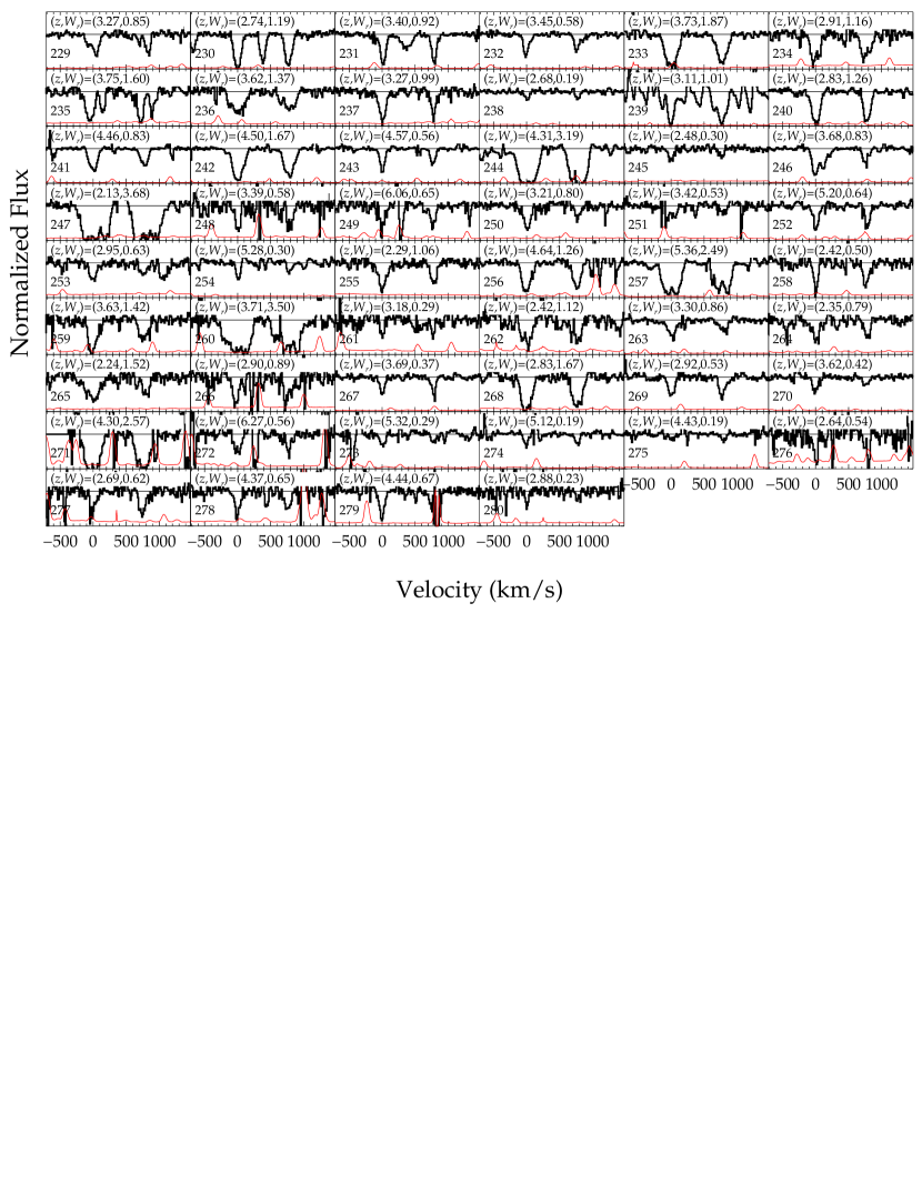
Figure 2.— Full Mg ii doublet sample identified in our survey, plotted as continuum-normalized spectra against velocity separation from the $2796\AA$ transition. The spectra are plotted on a linear scale from zero (bottom of plot) with the thin black line in each panel denoting unity. All doublets are shown in the order presented in Table 2, with index number at lower left of each panel corresponding to the rown number in the Table. The thin red line in each panel indicates the $1\sigma$ error in normalized flux for each pixel.

Table 2Summary of Absorption Properties for the FIRE Mg ii Sample

Index #	Sightline	$z$	$W_{r}(2796)$	$\sigma(2796)$	$\Delta v$
			(Å)	(Å)	(km s-1)
1	Q0000-26	2.1839	0.140	0.032	167.8
2	Q0000-26	3.3900	1.340	0.029	232.3
3	BR0004-6224	3.7765	0.988	0.054	193.8
4	BR0004-6224	3.2037	0.601	0.043	114.6
5	BR0004-6224	3.6946	0.250	0.047	154.7
6	BR0004-6224	2.9598	0.470	0.086	167.8
7	BR0016-3544	2.7825	0.566	0.034	180.8
8	BR0016-3544	3.7571	1.321	0.038	384.5
9	BR0016-3544	2.9485	0.146	0.031	86.7
10	BR0016-3544	2.8184	4.116	0.059	686.1
11	SDSS J0040-0915	4.4268	0.204	0.023	128.2
12	SDSS J0040-0915	4.7396	0.831	0.027	154.7
13	SDSS J0040-0915	2.6715	0.582	0.057	346.6
14	SDSS J0042-1020	3.6297	1.129	0.031	308.7
15	SDSS J0042-1020	2.7550	2.141	0.023	334.0
16	SDSS J0054-0109	4.9975	0.476	0.063	283.3
17	SDSS J0054-0109	2.4471	0.159	0.065	55.9
18	SDSS J0100+28	4.5192	0.834	0.029	308.7
19	SDSS J0100+28	5.3389	0.147	0.005	128.2
20	SDSS J0100+28	3.3376	0.286	0.021	114.6
21	SDSS J0100+28	5.1084	1.300	0.014	193.8
22	SDSS J0100+28	3.0515	0.151	0.012	167.8
23	SDSS J0100+28	4.2230	1.971	0.035	598.3
24	SDSS J0100+28	2.3255	1.364	0.009	180.8
25	SDSS J0100+28	4.3479	0.060	0.008	167.8
26	SDSS J0100+28	6.1437	0.415	0.006	86.7
27	SDSS J0100+28	2.9001	0.114	0.005	128.2
28	SDSS J0100+28	2.5620	0.147	0.009	114.6
29	SDSS J0100+28	2.5819	0.098	0.011	232.3
30	SDSS J0100+28	2.7501	0.264	0.009	167.8
31	SDSS J0100+28	4.6435	0.149	0.010	114.6
32	SDSS J0100+28	6.1118	0.300	0.005	114.6
33	SDSS J0106+0048	3.7290	0.854	0.016	154.7
34	VIK J0109-3047	2.9695	0.454	0.074	100.8
35	VIK J0109-3047	5.0011	0.335	0.042	128.2
36	SDSS J0113-0935	3.6167	0.581	0.046	180.8
37	SDSS J0113-0935	3.5446	0.231	0.039	128.2
38	SDSS J0113-0935	3.1140	0.257	0.031	141.5
39	SDSS J0113-0935	2.8252	0.188	0.029	114.6
40	SDSS J0127-0045	1.9785	0.168	0.021	296.0
41	SDSS J0127-0045	3.7282	0.863	0.014	167.8
42	SDSS J0127-0045	3.1688	0.270	0.019	346.6
43	SDSS J0127-0045	2.5881	1.568	0.027	535.5
44	SDSS J0127-0045	2.9458	2.272	0.040	397.1
45	SDSS J0140-0839	2.2408	0.415	0.027	141.5
46	SDSS J0140-0839	3.2122	0.093	0.014	141.5
47	SDSS J0140-0839	3.0815	0.565	0.021	114.6
48	SDSS J0157-0106	3.3860	1.332	0.083	409.7
49	SDSS J0157-0106	2.6311	0.734	0.079	206.7
50	SDSS J0157-0106	2.7980	0.510	0.052	359.3
51	PSO J029-29	4.8762	0.289	0.028	114.6
52	PSO J029-29	3.6086	1.219	0.054	180.8
53	PSO J029-29	4.9864	2.966	0.102	472.7
54	ULAS J0203+0012	3.7110	0.267	0.045	154.7
55	ULAS J0203+0012	4.3129	0.830	0.095	154.7
56	ULAS J0203+0012	4.9770	0.916	0.105	193.8
57	ULAS J0203+0012	4.4818	0.548	0.195	128.2
58	SDSS J0216-0921	2.4363	0.433	0.056	232.3
59	SDSS J0231-0728	5.3391	0.699	0.056	296.0
60	SDSS J0231-0728	3.1113	0.518	0.052	86.7

Table 2Summary of Absorption Properties for the FIRE Mg ii Sample (Continued)

Index #	Sightline	$z$	$W_{r}(2796)$	$\sigma(2796)$	$\Delta v$
			(Å)	(Å)	(km s-1)
61	SDSS J0231-0728	4.8840	1.322	0.133	409.7
62	SDSS J0231-0728	3.4298	0.431	0.037	167.8
63	ATLAS J025-33	5.3153	1.007	0.050	154.7
64	ATLAS J025-33	2.6666	0.470	0.024	154.7
65	ATLAS J025-33	2.7340	0.591	0.017	128.2
66	ATLAS J025-33	2.4460	2.183	0.031	409.7
67	BR0305-4957	3.3545	0.576	0.016	154.7
68	BR0305-4957	2.5023	0.322	0.027	206.7
69	BR0305-4957	2.6295	1.127	0.021	245.1
70	BR0305-4957	4.4669	1.789	0.016	283.3
71	BR0305-4957	4.2120	2.047	0.018	761.4
72	BR0305-4957	3.5916	1.503	0.020	232.3
73	VIK J0305-3150	2.4962	2.707	0.122	397.1
74	VIK J0305-3150	4.6202	0.401	0.040	128.2
75	VIK J0305-3150	2.5652	2.638	0.124	573.2
76	VIK J0305-3150	3.4650	0.256	0.035	100.8
77	BR0322-2928	2.2291	0.617	0.023	128.2
78	BR0331-1622	2.5933	0.230	0.024	100.8
79	BR0331-1622	2.2952	1.804	0.076	460.1
80	BR0331-1622	2.9277	1.311	0.055	359.3
81	BR0331-1622	3.5566	0.714	0.039	154.7
82	SDSS J0332-0654	3.0618	0.686	0.113	245.1
83	SDSS J0338+0021	2.2947	1.103	0.091	128.2
84	BR0353-3820	1.9871	3.142	0.036	548.1
85	BR0353-3820	2.7537	4.519	0.020	824.0
86	BR0353-3820	2.6965	0.357	0.018	180.8
87	PSO J036+03	4.6947	0.295	0.027	167.8
88	PSO J036+03	3.2745	0.710	0.028	180.8
89	BR0418-5723	2.9780	1.896	0.080	334.0
90	BR0418-5723	2.0305	1.533	0.074	245.1
91	DES0454-4448	2.5264	1.566	0.050	257.9
92	DES0454-4448	2.3174	2.350	0.047	384.5
93	DES0454-4448	3.7234	0.407	0.048	180.8
94	DES0454-4448	3.3932	0.842	0.082	206.7
95	DES0454-4448	3.5017	0.176	0.043	100.8
96	DES0454-4448	3.4500	0.582	0.020	128.2
97	DES0454-4448	2.7565	0.370	0.023	114.6
98	PSO J065-26	3.5381	1.923	0.133	346.6
99	PSO J065-26	3.4480	1.902	0.029	257.9
100	PSO J065-26	2.9829	1.315	0.070	257.9
101	PSO J071-02	2.7732	0.747	0.042	167.8
102	PSO J071-02	4.9944	1.059	0.073	257.9
103	PSO J071-02	5.1735	2.738	0.111	371.9
104	SDSS J0817+1351	2.9946	1.185	0.102	232.3
105	SDSS J0817+1351	3.4648	0.293	0.055	193.8
106	SDSS J0818+0719	2.2049	0.353	0.047	193.8
107	SDSS J0818+0719	2.0832	0.217	0.028	167.8
108	SDSS J0818+1722	3.5629	0.607	0.078	128.2
109	SDSS J0818+1722	5.0649	0.834	0.063	128.2
110	SDSS J0818+1722	4.4309	0.478	0.053	180.8
111	SDSS J0824+1302	2.7919	0.327	0.055	154.7
112	SDSS J0824+1302	4.8110	0.224	0.035	100.8
113	SDSS J0824+1302	3.5872	0.234	0.071	86.7
114	SDSS J0824+1302	4.4716	0.866	0.027	167.8
115	SDSS J0824+1302	4.8308	0.659	0.047	114.6
116	SDSS J0836+0054	2.2990	0.565	0.022	232.3
117	SDSS J0836+0054	3.7443	2.509	0.016	510.4
118	SDSS J0842+1218	5.0481	1.813	0.146	245.1
119	SDSS J0842+1218	2.3921	1.437	0.251	193.8
120	SDSS J0842+1218	2.5397	2.157	0.098	384.5

Table 2Summary of Absorption Properties for the FIRE Mg ii Sample (Continued)

Index #	Sightline	$z$	$W_{r}(2796)$	$\sigma(2796)$	$\Delta v$
			(Å)	(Å)	(km s-1)
121	SDSS J0949+0335	3.3105	2.026	0.044	296.0
122	SDSS J0949+0335	2.2888	2.834	0.065	472.7
123	SDSS J1015+0020	2.0588	3.161	0.133	510.4
124	SDSS J1015+0020	3.1040	3.862	0.072	773.9
125	SDSS J1015+0020	2.7103	1.417	0.073	296.0
126	SDSS J1015+0020	3.7299	0.489	0.029	141.5
127	SDSS J1020+0922	3.4786	0.117	0.016	128.2
128	SDSS J1020+0922	2.7485	0.635	0.024	141.5
129	SDSS J1020+0922	2.5933	0.482	0.027	128.2
130	SDSS J1020+0922	2.0461	0.381	0.046	114.6
131	SDSS J1030+0524	2.1881	0.315	0.021	371.9
132	SDSS J1030+0524	4.5836	1.839	0.033	321.3
133	SDSS J1030+0524	4.9481	0.455	0.023	141.5
134	SDSS J1030+0524	5.1307	0.146	0.013	55.9
135	SDSS J1037+0704	3.1373	0.349	0.062	193.8
136	J1048-0109	6.2215	1.647	0.163	232.3
137	J1048-0109	3.7465	0.952	0.061	167.8
138	J1048-0109	4.8206	0.890	0.037	154.7
139	J1048-0109	3.4968	2.221	0.076	434.9
140	J1048-0109	3.4133	0.547	0.031	167.8
141	SDSS J1100+1122	3.7566	1.342	0.055	232.3
142	SDSS J1100+1122	2.7825	0.691	0.054	193.8
143	SDSS J1100+1122	2.8225	0.570	0.063	206.7
144	SDSS J1100+1122	4.3959	1.866	0.101	257.9
145	SDSS J1101+0531	4.3431	3.118	0.264	460.1
146	SDSS J1101+0531	4.8902	0.346	0.074	154.7
147	SDSS J1101+0531	3.7191	0.820	0.063	257.9
148	SDSS J1110+0244	2.1188	2.957	0.043	460.1
149	SDSS J1110+0244	2.2232	0.193	0.024	141.5
150	SDSS J1115+0829	3.4045	0.731	0.034	154.7
151	SDSS J1115+0829	3.5427	1.557	0.172	219.5
152	SDSS J1115+0829	2.3209	0.359	0.037	55.9
153	ULAS J1120+0641	4.4725	0.298	0.015	128.2
154	ULAS J1120+0641	2.8004	0.178	0.041	71.9
155	SDSS J1132+1209	2.7334	0.180	0.031	206.7
156	SDSS J1132+1209	2.9568	1.210	0.072	206.7
157	SDSS J1132+1209	4.3801	0.968	0.098	193.8
158	SDSS J1132+1209	2.4541	0.333	0.049	180.8
159	SDSS J1132+1209	5.0162	0.249	0.027	114.6
160	ULAS J1148+0702	4.3673	4.784	0.112	371.9
161	ULAS J1148+0702	2.3858	2.600	0.287	359.3
162	ULAS J1148+0702	3.4936	4.822	0.194	899.2
163	PSO J183-12	4.8709	0.503	0.019	114.6
164	PSO J183-12	2.1068	0.710	0.024	245.1
165	PSO J183-12	2.2972	0.341	0.021	100.8
166	PSO J183-12	2.4058	0.225	0.030	128.2
167	PSO J183-12	2.4308	1.574	0.023	346.6
168	PSO J183-12	3.3956	1.069	0.032	283.3
169	SDSS J1253+1046	4.7930	0.394	0.052	100.8
170	SDSS J1253+1046	3.0282	1.010	0.037	193.8
171	SDSS J1253+1046	2.8565	0.169	0.030	100.8
172	SDSS J1253+1046	4.6004	0.882	0.108	154.7
173	SDSS J1257-0111	2.4894	0.223	0.019	154.7
174	SDSS J1257-0111	2.9181	0.955	0.020	180.8
175	SDSS J1305+0521	2.7527	0.375	0.040	128.2
176	SDSS J1305+0521	2.3023	1.976	0.122	346.6
177	SDSS J1305+0521	3.2354	0.337	0.026	128.2
178	SDSS J1305+0521	3.6799	1.749	0.069	270.6
179	SDSS J1306+0356	3.4898	0.607	0.033	167.8
180	SDSS J1306+0356	2.5328	2.813	0.115	535.5

Table 2Summary of Absorption Properties for the FIRE Mg ii Sample (Continued)

Index #	Sightline	$z$	$W_{r}(2796)$	$\sigma(2796)$	$\Delta v$
			(Å)	(Å)	(km s-1)
181	SDSS J1306+0356	4.8651	2.804	0.068	180.8
182	SDSS J1306+0356	4.6147	0.547	0.089	128.2
183	ULAS J1319+0950	4.5681	0.420	0.062	128.2
184	SDSS J1402+0146	3.2772	1.085	0.021	180.8
185	SDSS J1408+0205	2.4622	1.349	0.047	219.5
186	SDSS J1408+0205	1.9816	2.174	0.063	334.0
187	SDSS J1408+0205	1.9910	0.830	0.038	219.5
188	SDSS J1411+1217	5.0552	0.193	0.016	86.7
189	SDSS J1411+1217	2.2367	0.647	0.040	193.8
190	SDSS J1411+1217	5.2501	0.295	0.015	128.2
191	SDSS J1411+1217	5.3315	0.182	0.016	100.8
192	SDSS J1411+1217	3.4773	0.343	0.020	86.7
193	SDSS J1411+1217	4.9285	0.659	0.024	128.2
194	PSO J213-02	4.9125	0.623	0.030	128.2
195	PSO J213-02	4.7777	0.295	0.028	114.6
196	Q1422+2309	1.9720	0.163	0.020	128.2
197	SDSS J1433+0227	2.7717	0.726	0.018	128.2
198	SDSS J1436+2132	2.9070	4.309	0.030	610.9
199	SDSS J1436+2132	4.5211	0.964	0.166	193.8
200	SDSS J1444-0101	4.4690	2.002	0.173	472.7
201	SDSS J1444-0101	2.8103	0.599	0.059	141.5
202	SDSS J1444-0101	2.7967	0.264	0.044	114.6
203	CFQS1509-1749	3.2662	0.940	0.018	180.8
204	CFQS1509-1749	3.1272	0.878	0.076	245.1
205	CFQS1509-1749	3.3925	5.679	0.056	811.5
206	SDSS J1511+0408	2.0394	2.978	0.090	359.3
207	SDSS J1511+0408	2.2771	2.756	0.081	485.3
208	SDSS J1511+0408	3.3588	1.464	0.067	397.1
209	SDSS J1511+0408	2.2310	1.825	0.051	321.3
210	SDSS J1511+0408	2.0230	1.129	0.053	232.3
211	SDSS J1532+2237	2.6116	1.725	0.032	245.1
212	SDSS J1532+2237	2.7414	0.862	0.033	283.3
213	SDSS J1538+0855	3.4979	0.165	0.012	346.6
214	SDSS J1538+0855	2.6383	0.282	0.027	154.7
215	PSO J159-02	6.2376	0.458	0.045	257.9
216	PSO J159-02	2.2465	0.163	0.027	71.9
217	PSO J159-02	3.6695	2.269	0.115	460.1
218	PSO J159-02	3.7422	0.681	0.047	257.9
219	PSO J159-02	6.0549	0.436	0.065	167.8
220	PSO J159-02	4.3426	0.222	0.046	141.5
221	SDSS J1601+0435	3.5007	1.467	0.129	308.7
222	SDSS J1606+0850	2.7636	3.433	0.128	548.1
223	SDSS J1606+0850	4.4426	0.464	0.041	100.8
224	SDSS J1611+0844	3.7767	0.801	0.053	206.7
225	SDSS J1611+0844	2.0144	0.506	0.059	100.8
226	SDSS J1611+0844	3.1454	2.662	0.213	422.3
227	SDSS J1611+0844	3.3861	0.464	0.038	141.5
228	SDSS J1616+0501	1.9809	2.115	0.050	270.6
229	SDSS J1616+0501	3.2747	0.853	0.021	180.8
230	SDSS J1616+0501	2.7409	1.188	0.026	193.8
231	SDSS J1616+0501	3.3955	0.916	0.055	141.5
232	SDSS J1616+0501	3.4507	0.584	0.017	128.2
233	SDSS J1616+0501	3.7327	1.866	0.057	321.3
234	SDSS J1620+0020	2.9106	1.159	0.055	270.6
235	SDSS J1620+0020	3.7515	1.601	0.070	232.3
236	SDSS J1620+0020	3.6200	1.366	0.066	397.1
237	SDSS J1620+0020	3.2726	0.988	0.047	167.8
238	SDSS J1621-0042	2.6780	0.189	0.019	100.8
239	SDSS J1621-0042	3.1057	1.013	0.013	232.3
240	SDSS J1626+2751	2.8288	1.260	0.041	206.7

Table 2Summary of Absorption Properties for the FIRE Mg ii Sample (Continued)

Index #	Sightline	$z$	$W_{r}(2796)$	$\sigma(2796)$	$\Delta v$
			(Å)	(Å)	(km s-1)
241	SDSS J1626+2751	4.4619	0.829	0.014	219.5
242	SDSS J1626+2751	4.4968	1.673	0.019	283.3
243	SDSS J1626+2751	4.5682	0.561	0.025	128.2
244	SDSS J1626+2751	4.3108	3.188	0.050	434.9
245	SDSS J1626+2751	2.4822	0.300	0.032	141.5
246	SDSS J1626+2751	3.6826	0.833	0.011	167.8
247	SDSS J1626+2751	2.1320	3.679	0.091	321.3
248	PSO J167-13	3.3889	0.581	0.036	141.5
249	PSO J183+05	6.0643	0.653	0.096	141.5
250	PSO J183+05	3.2071	0.803	0.042	180.8
251	PSO J183+05	3.4184	0.533	0.077	219.5
252	PSO J209-26	5.2021	0.643	0.025	154.7
253	PSO J209-26	2.9505	0.631	0.048	206.7
254	PSO J209-26	5.2758	0.299	0.020	100.8
255	SDSS J2147-0838	2.2863	1.058	0.049	206.7
256	PSO J217-16	4.6420	1.261	0.044	219.5
257	PSO J217-16	5.3571	2.489	0.029	359.3
258	PSO J217-16	2.4166	0.501	0.050	128.2
259	VIK J2211-3206	3.6302	1.416	0.092	257.9
260	VIK J2211-3206	3.7144	3.505	0.068	623.4
261	SDSS J2228-0757	3.1754	0.287	0.038	71.9
262	PSO J231-20	2.4191	1.115	0.090	257.9
263	SDSS J2310+1855	3.2998	0.856	0.058	257.9
264	SDSS J2310+1855	2.3510	0.789	0.052	193.8
265	SDSS J2310+1855	2.2430	1.523	0.068	334.0
266	VIK J2318-3113	2.9030	0.887	0.075	219.5
267	BR2346-3729	3.6922	0.371	0.019	128.2
268	BR2346-3729	2.8300	1.665	0.054	270.6
269	BR2346-3729	2.9226	0.535	0.041	167.8
270	BR2346-3729	3.6188	0.422	0.036	141.5
271	VIK J2348-3054	4.2996	2.567	0.118	384.5
272	VIK J2348-3054	6.2682	0.564	0.062	167.8
273	PSO J239-07	5.3238	0.287	0.024	141.5
274	PSO J239-07	5.1209	0.193	0.022	114.6
275	PSO J239-07	4.4276	0.193	0.018	141.5
276	PSO J242-12	2.6351	0.543	0.075	114.6
277	PSO J242-12	2.6880	0.620	0.087	180.8
278	PSO J242-12	4.3658	0.646	0.086	154.7
279	PSO J242-12	4.4351	0.671	0.041	141.5
280	PSO J308-27	2.8797	0.229	0.032	71.9
$\cdots$	BR0004-6224	2.663	0.260	0.045	58.0
$\cdots$	BR0004-6224	2.908	0.596	0.047	83.3
$\cdots$	SDSS J1030+0525	2.780	2.617	0.069	583.9
$\cdots$	SDSS J1306+0356	4.882	1.941	0.079	248.8
$\cdots$	SDSS J1402+0146	3.454	0.341	0.016	173.3
$\cdots$	Q1422+2309	3.540	0.169	0.011	130.0
$\cdots$	SDSS J2310+1855	2.243	1.441	0.050	292.1

Table 3Proximate Mg ii Systems

Index #	Sightline	$z$	$W_{r}(2796)$	$\sigma(2796)$	$\Delta v$
			(Å)	(Å)	(km s-1)
1	PSO J065-26	6.122	2.346	0.038	553.4
2	SDSS J0140-0839	3.703	0.584	0.015	216.0
3	SDSS J1436+2132	4.522	0.973	0.189	332.8
4	SDSS J1626+2751	5.178	1.416	0.022	518.6
5	PSO J183+05	6.404	0.774	0.053	356.6

For consistency, we have redone the line finding for the sightlines presented in Paper I. A complete list of these doublets and their continuum-normalized profiles are included in Table 2 and Figure 2, respectively. Differences in user acceptances/rejections are noted in the table: in general, as the visual inspection step was carried out by a different user than in the original survey (SC and MM, respectively), we tended to be more optimistic in accepting borderline candidates for Mg ii doublets. These tendencies are reflected in the user-rating calibration, discussed below. In addition, we serendipitously identified five systems excluded by the automated search algorithm. These are reported and flagged in the table of absorbers, but they are omitted from calculations of the Mg ii population statistics, because the statistical calculations account for such missed systems via incompleness simulations. In the process of the visual identification, we also identified five Mg ii absorbers which were not included in our sample due to their proximity to the background quasar; these are listed with their associated properties in Table 3. The proximate absorbers in the two PS1 quasars are of particular interest and will be discussed in detail in forthcoming work (Banados, 2017).

3.3. Automated Completeness Test

We ran a large Monte Carlo simulation to quantify the the completeness of the automated line-finding algorithm. For each QSO, 10,000 simulated Mg ii doublets with equivalent widths uniformly distributed between 0.05 and 0.95 Å and random redshifts were injected into the spectrum (from which the real doublets were previously removed and replaced with noise) and then subjected to the automated line-finding algorithm. The rates at which these simulated doublets were recovered were then binned into an automated completeness grid by redshift and equivalent width (with $dz=0.02$ and $dW=0.01$ Å) for each QSO, which we will call $L_{q}(z,W)$. These computationally intensive simulations were run on the antares computing cluster at the MIT Kavli Institute.

3.4. User-Rating Calibration

A subset of the automatically simulated doublets were inspected visually to evaluate the efficacy of the human inspection step in our doublet-finding procedure. In particular, the user may either reject a real Mg ii system or accept a false positive, thus requiring a correction to our statistical calculations. We inspected 1000 such simulated doublets, with the important difference that the user-test systems had a slightly larger velocity spacing than legitimate Mg ii doublets. This ensures that any “doublets” identified by the machine are either artifically injected (and should therefore be accepted) or correlated noise (and should be rejected).

While inspecting these false-spacing doublets, we identified three very large absorbers, likely not due to Mg ii. These were manually excised and masked from our Monte Carlo data so that only injected doublets and correlated noise factored into the user ratings calculation. The user then either accepted or rejected the remaining candidate doublets, and the success rates at which the user identified real systems and rejected false positives were used to calculate a total completeness for each QSO.

As discussed in Paper I, the time-consuming nature of visual inspection precludes the use of finely grained bins in $W_{r}$ and $z$, but we found that the acceptance rate for real systems and false positives depended primarily on the SNR of the candidate doublets. They can be parametrized with SNR as follows:

$$P^{\rm MgII}(s)=P_{\infty}(1-e^{-s/s_{c}})$$ (1)

$$P^{\rm FP}(s)=\begin{cases}P^{\rm FP}_{\rm max}(\frac{s}{s_{p}}),\quad s\leq s_{p}\\ P^{\rm FP}_{\rm max}(\frac{s-s_{f}}{s_{p}-s_{f}}),\quad s>s_{p}\end{cases},$$ (2)

where $P^{\rm MgII}$ and $P^{\rm FP}$ are the acceptance rates for real systems and false positives, respectively, and $P_{\infty}$, $s_{c}$, $P^{\rm FP}_{\rm max}$, $s_{p},$ and $s_{f}$ are free parameters fit by maximum-likelihood estimation (MLE). Plots of the user acceptance rates are given in Figure 3. Comparing the ratings of SC and MM it is apparent that SC correctly identified a higher fraction of Mg ii doublets at low SNR, but this comes at the expense of a higher false-positive rate. After proper calibration these tendencies should cancel, and indeed we will find very similar statistical results as Paper I in areas where both may be compared.

Figure 3.— The user acceptance rates for real injected systems (top) and false positives (bottom), binned by the detection SNR for each doublet (i.e. the significance of the peak in cross-correlation between data and matched filter). The error bars represent the Wilson score interval, and the lines are the MLE fits for these rates. In the bottom panel, the errors are larger at high SNR because fewer injected systems are detected at SNR¿10 in the presence of noise.

For each individual QSO, the user-acceptance rates were then estimated as functions of the equivalent width $W_{r}$ to give $A^{\rm MgII}(W,z)$ and $A^{\rm FP}(W,z)$, the acceptance rates for real systems and false positives, respectively. The total completeness fraction for each QSO $q$, $C_{q}(z,W)$, was then calulated as the product of the automated completeness fraction and the user acceptance rate, namely

$$C_{q}(z,W)=A^{\rm MgII}(z,W)L_{q}(z,W).$$ (3)

The total pathlength-weighted completeness for our survey, thus calculated, is shown in Figure 4. The acceptance rate for false positives are not included in this step, but rather are accounted for directly in our calculations of the population statistics. Unlike in Paper I, the grid now extends to a maximum redshift of $z=7$, picking up path at $z>6.1$ where Mg ii re-emerges into the $K$-band atmospheric window.

Given the completeness grid calculated above, we can calculate the redshift path density $g(z,W)$ of our survey, i.e. the total number of sightlines at redshift $z$ for which Mg ii absorbers with equivalent width greater than $W_{r}$ can be observed, as

$$g(z,W)=\sum_{q}R_{q}(z)C_{q}(z,W),$$ (4)

where $R_{q}(z)$ is equal to one within the redshift search limits but outside the redshifts excluded due to poor telluric corrections, and zero everywhere else. This function is shown in the top panel of Figure 5; the bottom panel indicates the survey path $g(W)$, defined as

$$g(W)=\int g(z,W)dz$$ (5)

Here, the increase in completeness toward higher $W_{r}$ is reflected in the rising path probed at larger equivalent width. The converged value at $g(W)\sim 150$ toward large equivalent width indicates a high completeness, and an average redshift coverage of $\Delta z\sim 1.5$ per sightline for our 100 objects. The total survey path of Paper I was approximately 80, so we have roughly doubled the path by doubling the number of QSOs observed.

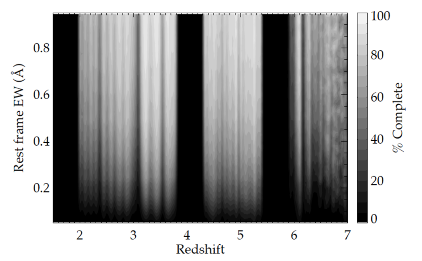
Figure 4.— The total pathlength-weighted completeness for our survey. Note the additional pathlength between redshifts z = 6 and 7, which is absent from Paper I on account of its smaller sample size and lack of $z>6.5$ background quasars. The broad completeness gaps centered at $z=4.0$ and $z=5.8$ mark the absorption bands between $J/H$, and $H/K$, respectively.

Figure 5.— Top: The completeness-weighted number of sightlines $g(z)$ that probe the sample’s redshift extent for three choices of $W_{R,2796}$: 0.3, 0.5, and 1.0Å. Bottom: Total absorption path as a function of limiting $W_{r,2796}$. These paths roughly double the survey volume probed by Paper I, shown as the dashed line in the bottom figure.

4. Results

Using these methods, we identified 280 Mg ii absorbers, not including any corrections for incompleteness. Histograms of the raw counts of these systems based on redshift and equivalent width are given in Figure 6. Detailed properties of each absorber are listed in Table 2.

Figure 6.— Raw counts of Mg ii absorbers found in our survey, binned by equivalent width and redshift. These numbers are not completeness corrected.

4.1. Accounting for Completeness and False Positives

We employed the same formalism described in Paper I, to account for incompleteness and false positives in our statistical results. Briefly, in a given redshift and equivalent width bin $k$, the corrected (true) number of systems can be calculated from the number $\breve{N}_{k}$ of detected systems in that bin as

$$N_{k}=\frac{\breve{N}_{k}(1-\bar{A}^{F}_{k})-\bar{A}^{F}_{k}\breve{F}_{k}}{\bar{C}_{k}-\bar{L}_{k}\bar{A}^{F}_{k}},$$ (6)

where $\breve{F}^{k}$ is the number of rejected candidates, $\bar{C}_{k}$ is the average completeness, $\bar{L}_{k}$ is the automated line identification finding probability, and $\bar{A}^{F}_{k}$ is the user-acceptance rate for false positives, each calculated for the kth bin. These fractions are calculated from the previously discussed automated completeness tests and user-rating calibrations. An important caveat is that the average completeness of a redshift and equivalent width bin is weighted according to the number distribution $d^{2}N/dzdW$, which must in principle be determined from the true number of systems $N_{k}$. Here we follow the discussion in Paper I and apply the simplifying assumption that $d^{2}N/dzdW$ is constant across each bin to resolve the apparent circularity.

4.2. The $W_{r}$ Frequency Distribution

Table 4Mg ii Equivalent Width Distribution,
Full Sample and Redshift Cuts

$z=1.90-6.30$
0.42 0.05-0.64 46.0 130 1.539$\pm$0.215
0.94 0.64-1.23 77.7 66 0.591$\pm$0.082
1.52 1.23-1.82 79.7 34 0.298$\pm$0.055
2.11 1.82-2.41 79.7 21 0.185$\pm$0.042
2.70 2.41-3.00 79.7 15 0.134$\pm$0.035
4.39 3.00-5.78 79.7 14 0.026$\pm$0.007

$z=1.95-2.98$
0.42 0.05-0.64 42.0 56 1.371$\pm$0.336
0.94 0.64-1.23 74.4 19 0.410$\pm$0.108
1.52 1.23-1.82 76.7 14 0.308$\pm$0.089
2.11 1.82-2.41 76.7 9 0.205$\pm$0.071
2.70 2.41-3.00 76.7 8 0.187$\pm$0.067
4.39 3.00-5.78 76.7 7 0.033$\pm$0.013

$z=3.15-3.81$
0.41 0.05-0.64 54.8 31 1.183$\pm$0.284
0.94 0.64-1.23 85.5 22 0.691$\pm$0.152
1.53 1.23-1.82 87.1 12 0.370$\pm$0.109
2.12 1.82-2.41 87.1 6 0.182$\pm$0.076
2.71 2.41-3.00 87.1 1 0.031$\pm$0.031
4.39 3.00-5.78 87.1 3 0.020$\pm$0.011

$z=4.34-5.35$
0.41 0.05-0.64 52.1 32 1.840$\pm$0.397
0.94 0.64-1.23 84.8 18 0.719$\pm$0.176
1.53 1.23-1.82 86.6 6 0.236$\pm$0.097
2.12 1.82-2.41 86.6 3 0.118$\pm$0.069
2.71 2.41-3.00 86.6 3 0.118$\pm$0.069
4.39 3.00-5.78 86.6 1 0.008$\pm$0.008

$z=6.00-7.08$
0.93 0.05-1.53 52.7 6 0.979$\pm$0.446
2.26 1.53-3.00 68.2 1 0.131$\pm$0.132
4.39 3.00-5.78 68.2 0 $<$0.070

Figure 7.— Population equivalent width density across the full survey redshift range. The dashed line indicates a MLE fit for an exponential distribution.

Figure 8.— Population equivalent width distribution at different redshift intervals. The dashed lines indicate MLE fits for an exponential distribution at these intervals. For comparison, the low redshift distribution from $z=1$, taken from Seyffert et al. (2013), is plotted in dotted line.

Table 4.2 lists completeness-corrected values for the rest equivalent width frequency distribution $d^{2}N/dzdW$, an absorption line analog of the galaxy luminosity function. These values are plotted in Figure 7 and Figure 8, where the equivalent width distribution is binned across the full survey redshift range and them split into four redshift intervals, respectively. The error bars for each point account both for Poisson fluctuations in the number count in each bin (which dominate the error budget), and for uncertainty in the completeness-adjusted path length. The latter term reflects errors in our completeness estimates, which are much smaller by design because of the large number of simulated doublets in the completeness and user rejection tests.

With only seven systems in the highest redshift bin, the fractional errors on each point and the associated fit parameters are large. However one can read off from these figures that the density of lines at $W_{r}<1$Å even at $z>6$ is quite comparable to lower redshift. At higher equivalent width ($W_{r}\gtrsim 2$Å) there is weak indication of a deficit compared with lower redshift, but the statistical errors on these points are significant and the fit parameterizations should therefore be interpreted with caution.

We fit the equivalent width distrbution using maximum likelihood estimation to the exponential form

$$\frac{d^{2}N}{dzdW}=\frac{N_{\ast}}{W_{\ast}}e^{-W/W_{\ast}}$$ (7)

by first fitting $W_{\ast}$ then setting the overall normalization $N_{\ast}$ such that the calculated number of systems in our survey is recovered. These fits are plotted as dashed lines in the figure of the frequency distribution. A list of the fit parameters are given in Table 4.2.

Table 5Maximum-Likelihood Fit Parameters for
Exponential Parameterization of the $W_{r}$ Distribution

0.68 & 0.366-0.871 0.585$\pm$0.024 1.216$\pm$0.124
1.10 0.871-1.311 0.741$\pm$0.032 1.171$\pm$0.083
1.60 1.311-2.269 0.804$\pm$0.034 1.267$\pm$0.092
2.52 1.947-2.975 0.840$\pm$0.092 2.226$\pm$0.081
3.46 3.150-3.805 0.806$\pm$0.105 1.864$\pm$0.069
4.80 4.345-5.350 0.618$\pm$0.097 2.227$\pm$0.131
6.29 5.995-7.080 0.500$\pm$0.148 2.625$\pm$0.452
3.47 1.947-6.207 0.798$\pm$0.055 2.051$\pm$0.046

Figure 9.— The characteristic equivalent width parameter $W_{\ast}$ plotted by redshift. The triangles are the points from this survey, while the boxes and crosses show the same parameter for lower redshifts from Seyffert et al. (2013) and Nestor et al. (2005), respectively. The dashed line gives the MLE fit for this parameter from Nestor et al. (2005) for the low redshift points.

Figure 9 displays evolution in the characteristic equivalent width $W_{\ast}$ with redshift. For comparison, we have added the equivalent parameters provided in Nestor et al. (2005) and Seyffert et al. (2013) at lower redshifts, though it is important to note that Seyffert et al. only include systems with $W_{r}>1$ Å in their fits. Throughout the analysis below we use these two samples as our low-redshift refrences even though many other Mg ii surveys have been performed on the SDSS QSO sample (Prochter et al., 2006; Lundgren et al., 2009; Quider et al., 2011; Zhu & Ménard, 2013; Chen et al., 2015; Raghunathan et al., 2016). The main motivation for our choice is that Nestor et al. (2005) probes the smallest equivalent widths (comparable to our measurements) in the SDSS data, while Seyffert et al. (2013) uses identification and analysis techniques most similar to our methods. However these results are broadly consistent with other works in the literature where they may be compared.

Our results confirm the trend noted in Paper I: at higher redshifts $W_{\ast}$ does not continue its growth with redshift at earlier times. Rather, it peaks at around $z=2$-$3$, after which it begins to decline. In direct terms, this corresponds to a similar peak in the incidence of strong Mg ii absorbers around $z=2$-$3$, with a dropoff toward early epochs in the strong systems relative to their weaker counterparts.

4.3. dN/dz and dN/dX

Figure 10.— The line density of Mg ii absorbers plotted by redshift, separated into three equivalent width ranges. Also plotted are the corresponding points at earlier redshift from Seyffert et al. (2013, small black points) ,Nestor et al. (2005, hollow triangles), and Churchill (2001, holllow squares). Dashed lines give the MLE fits for a power law distribution on our high redshift data.

Figure 11.— The comoving line density of Mg ii absorbers plotted by redshift, separated into different equivalent width ranges corresponding to weak and strong absorption systems. Also plotted are the corresponding points at earlier redshift from Seyffert et al. (2013, small black points) ,Nestor et al. (2005, hollow triangles), and Churchill (2001, holllow squares). The dashed line indicates a constant comoving population.

The zeroth moment of the frequency distribution gives the line density of Mg ii absorption lines $dN/dz$, as plotted in Figure 10. We include low-redshift points from Mg ii surveys of the SDSS (Nestor et al., 2005; Seyffert et al., 2013) for comparison. For completeness we have also performed MLE fits of the form

$$\frac{dN}{dz}=N_{\ast}(1+z)^{\beta}$$ (8)

on our high redshift points, where the normalization $N_{\ast}$ is fixed such that $dN/dz$ integrated by redshift with the survey path density $g(z,W)$ recovers the number counts of our survey; these fits are shown as dashed lines in Figure 10. These results and parameter fits are listed in Table 6 and Table 7, respectively.

The line density $dN/dz$ can further be converted to the more physical comoving line density $dN/dX$. Here we divide the distribution into two equivalent width bins separated at $W_{r}=1$Å, and 5 redshift bins to illustrate differences in evolutionary trends.

As with the equivalent width distribution, error bars include a Poisson contribution from the number of systems in each bin, and an additional (much smaller) contribution from uncertainty in the completeness values used to adjust the survey pathlength ($dz$ or $dX$). The overall accuracy of the FIRE survey points is likely limited by statistical errors—even with 100 sightlines we average just 10-25 absorbers per bin, corresponding to a 20-30% uncertainty. In contrast the low redshift studies from SDSS have thousands of absorbers per redshift bin and therefore have errors dominated by systematic effects not explicitly quantified in these studies (and therefore not captured in the figure). As argued by Seyffert et al. (2013) these likely arise from differences in (a) continuum fitting procedures, and (b) algorithms for measuring $W_{r}$, and (c) use of a sharp $W_{r}$ cutoff when defining samples used to derive $dN/dX$. Comparison of different Mg ii surveys from SDSS QSOs suggests a systematic scatter of $\sim 10-15\%$, far larger than the $\sim 1\%$ random errors (Seyffert et al., 2013) These different errors must be considered when comparing in regions of overlap such as the bottom panel of Figure 11.

The larger survey confirms and strengthens two key findings of Paper I by both reducing Poisson errors on points at $z<5$, and adding new redshift coverage at $z>6$. First, the comoving absorption density (i.e. the frequency) of typical Mg ii systems with $0.3<W_{r}<1$Å remains remarkably constant from $z=0.5$ to $z=7$, i.e. all redshifts that have been searched.

This can only be true if the product of the comoving volume density of absorbers $n(z)$, multiplied by the physical cross section of each absorber $\sigma$, also remains a constant. If Mg ii absorbers at high redshift are associated with luminous galaxies like their low-redshift counterparts, then circum-galactic gas must therefore have a substantial cross-section for heavy-element absorption even very early in these galaxies’ evolutionary history. Our previous work suggested this result to $z=5.5$; the new sightlines presented here exhibit the exact number of Mg ii one would expect from simple extrapolation of this trend to $z=6.5$, when the universe was $850$ Myr old.

The second key finding from Paper I confirmed here is a firm evolution in the frequency of strong Mg ii absorbers at $W_{r}>1$Å. This trend is in marked contrast to the weaker systems, and is consistent with the evolution in $W^{*}$ of the frequency distribution $d^{2}N/dXdW$. We find just one strong system at $z>6$, again consistent with expectations extrapolated from lower $z$. The decline of nearly an order of magnitude from the peak at $z\sim 2.5$ suggests that further searches for strong systems at $z\sim 7$ and beyond are likely to require many sightlines toward faint QSOs; however the weaker systems may well remain plentiful.

Table 6Mg ii Absorption line density $dN/dz$

$\left<z\right>$	$\Delta z$	$\bar{C}$	Number	$dN/dz$	$dN/dX$
		$(\%)$
$0.3\textrm{\AA}<W_{r}<0.6$ Å
2.236	1.947-2.461	46.2	11	0.308$\pm$0.168	0.100$\pm$0.054
2.727	2.461-2.975	62.2	18	0.499$\pm$0.137	0.149$\pm$0.041
3.460	3.150-3.805	69.4	15	0.336$\pm$0.091	0.090$\pm$0.024
4.806	4.345-5.350	66.2	13	0.391$\pm$0.113	0.091$\pm$0.026
6.291	5.995-7.085	43.1	4	1.173$\pm$0.667	0.241$\pm$0.137
$0.6\textrm{\AA}<W_{r}<1.0\textrm{\AA}$
2.236	1.947-2.461	63.7	5	0.133$\pm$0.081	0.043$\pm$0.026
2.723	2.461-2.975	78.9	10	0.232$\pm$0.079	0.069$\pm$0.024
3.463	3.150-3.805	83.7	21	0.398$\pm$0.090	0.107$\pm$0.024
4.802	4.345-5.350	82.6	17	0.412$\pm$0.103	0.096$\pm$0.024
6.289	5.995-7.085	62.5	1	0.211$\pm$0.213	0.043$\pm$0.044
$W_{r}>1.0\textrm{\AA}$
2.236	1.947-2.461	68.7	24	0.751$\pm$0.172	0.244$\pm$0.056
2.722	2.461-2.975	83.4	22	0.505$\pm$0.113	0.150$\pm$0.034
3.463	3.150-3.805	87.1	26	0.471$\pm$0.096	0.127$\pm$0.026
4.801	4.345-5.350	86.6	15	0.346$\pm$0.092	0.081$\pm$0.022
6.287	5.995-7.085	68.2	1	0.193$\pm$0.195	0.040$\pm$0.040

Table 7Maximum-Likelihood Estimates of the
Line Density Evolution $dN/dz=N^{*}(1+z)^{\beta}$

$\left<W_{r}\right>$	$\Delta W_{r}$	$\Delta z$	$\beta$	$N^{*}$
(Å)	(Å)
1.17	1.00-1.40	0.35-2.3	$0.99^{+0.29}_{-0.22}$	$0.51^{+0.09}_{-0.10}$
1.58	1.40-1.80	0.35-2.3	$1.56^{+0.33}_{-0.31}$	$0.020^{+0.05}_{-0.05}$
1.63	1.00+	0.35-2.3	$1.40^{+0.16}_{-0.16}$	$0.08^{+0.15}_{-0.05}$
2.08	1.40+	0.35-2.3	$1.74^{+0.22}_{-0.22}$	$0.036^{+0.06}_{-0.06}$
2.52	1.80+	0.35-2.3	$1.92^{+0.30}_{-0.32}$	$0.016^{+0.06}_{-0.03}$
0.45	0.30-0.60	1.9-6.3	-0.345$\pm$0.616	0.722$\pm$0.653
0.79	0.60-1.00	1.9-6.3	0.821$\pm$0.505	0.090$\pm$0.069
1.80	1.00+	1.9-6.3	-1.020$\pm$0.475	2.298$\pm$1.561

4.4. Comparison with Other Searches for High-Redshift MgII

In the time since initial submission of this paper, two other relevant manuscripts have been posted describing Mg ii searches in the near-IR. We comment briefly here on comparisons of these studies with our work.

Codoreanu et al. (2017) searched a sample of four high-SNR spectra obtained with VLT/XShooter for Mg ii; because of the exceptional data quality this search is more sensitive to weak absorption lines but its shorter survey path length leads to larger Poisson uncertainties in bins of higher equivalent width. In the regions where our samples are best compared ($0.3<W_{r}<1.0$Å) the agreement in number density is very good. Our larger sample size reveals evidence for evolution at $W_{R}>1$Å not visible in their data; however, their higher sensitivity reveals numerous weak systems ($W_{r}<0.3$Å). While we report some such systems in Table 2, our overall completeness was not sufficient to claim robust statistics on these absorbers. Their analysis reveals an excess of weak Mg ii systems relative to an extrapolation of the exponential frequency distribution, as found at lower redshift. The trend of number density with redshift for these weak systems is broadly consistent with no evolution, though increased sample size could reveal underlying trends.

Separately, Bosman et al. (2017) performed an ultra-deep survey for Mg ii along the line of sight to ULAS1120+0641, also covered in our sample. They recover the two systems in our sample, and further recover three systems with $W_{r}<0.3$Å at $z>6$ not detected by our search (because of our lower SNR, particularly in regions of strong and/or blended telluric absorption and emission). The number of weak systems uncovered in this sightline tentatively suggests that the frequency distribution may transition to a power-law slope at low column densities where our survey would have correspondingly low completeness.

5. Discussion

We have extended the original survey of Paper I from 46 to 100 QSOs, with particular emphasis on increasing path length at higher redshift. While significantly augmenting the sample of Mg ii absorbers, we confirm the trends noted in Paper I. Our data (1) rule out the monotonic growth of $W_{\ast}$ at high redshifts and (2) show that the comoving line density of $W_{r}<1$Å Mg ii absorbers does not evolve within errors, while stronger absorbers demonstrate a noticeable decline in comoving line density. In particular, our detection of five Mg ii systems at $z>6$ with equivalent width $0.3<W_{r}<1.0$Å conforms with a constant comoving population ansatz for the weak Mg ii systems.

5.1. Strong Mg ii and the Global Star Formation Rate

In Paper I, we discussed the hypothesis that strong Mg ii absorption is linked closely with star forming galaxies, using the scaling relation presented in Ménard et al. (2011) to convert Mg ii equivalent widths into an effective contribution to the global star formation rate. This integral is dominated by the strongest absorbers in the sample, which peak strongly in number density near $z\sim 2$-$3$, similar to the SFR rate density.

The conversion method relies on a correlation observed in SDSS-detected Mg ii systems between $W_{r}$ and [O ii] luminosity surface density measured in the same fiber as the background QSO:

$$\left<{\Sigma_{L_{OII}}}\right>\propto\left({{W_{r}}\over{1{\rm\AA}}}\right)^{1.75}.$$ (9)

By integrating the Mg ii equivalent width distribution $d^{2}N/dWdX$, weighted by the function in Equation 9, one obtains a volumetric luminosity density of [O ii] which can then be converted into a star formation rate density using the [O ii]  - SFR scaling relations of Zhu et al. (2009). As discussed in Paper I, one should keep in mind the possibility raised by López & Chen (2012) that the correlation in Equation 9 could arise from the decline in $W_{r}$ with impact parameter, coupled with differential loss of [O ii] flux from the SDSS fiber, rather than a physical link between the SFR and Mg ii absorption strength. However in light of the observed evolution in $dN/dX$ for strong systems, the large velocity spreads seen in the strongest systems, and the link between star formation and Mg ii seen in individual galaxies (Bouché et al., 2007; Noterdaeme et al., 2010), we explore this possibility while acknowledging its possible limitations.

Figure 12 presents an updated version of this calculation, with smaller errors from our new and larger sample, and an additional point at $z>6$ from our new high redshift sightlines. Despite the caveats presented in Paper I about the methodology of the Mg ii -SFR conversion (López & Chen, 2012), and the application of low-redshift scalings at these early epochs, the agreement between the Mg ii-inferred SFR and the values measured directly from deep fields remains remarkable. This suggests that at least the strongest Mg ii systems in our surveys derive their large equivalent widths (i.e. their velocity structure) from processes connected to star formation.

Figure 12.— Comparison of the SFR density in units of comoving Mpc³, determined directly from observations of deep fields (triangles) and as converted from Mg ii absorber statistics using the prescription of Ménard et al. (2011). The coincidence remains in place with an increased sample size and the addition of a new point at higher redshift.

5.2. Low Mass Halos as Sites of Early Mg ii Absorption

The persistence of Mg ii at $dN/dX\approx 0.2$ absorbers per comoving path length at $z\sim 5.5$-$6.5$ merits further examination, because it implies that some CGM gas was enriched very early in cosmic history—indeed, well before galactic stellar populations were fully relaxed. In Paper I we explored whether known high-redshift galaxy populations could plausibly account for the observed number of Mg ii systems, supposing that radial scaling relations of $W_{r}$ and covering fraction measured at $z<0.5$ apply at early times. These calculations essentially integrate down a mass function or a luminosity function to obtain a number density of halos, and then seed these with Mg ii gas using a radial prescription. Mg ii absorption statistics calculated in this way are sensitive to the lower limit of integration, as well as the value assumed for the low-mass (or faint-end) slope.

In that work, we first examined the predictions of a halo-occupation distribution model from Tinker & Chen (2010a). These authors integrate the halo mass function down to a fixed, redshift-independent cutoff below which it is assumed that galaxies do not harbor Mg ii in their CGM. The cutoff is chosen to match the evolution in number statistics below $z<2$, but substantially underpredicts the Mg ii incidence rate at higher redshift. This likely results from the evolving mass function; since halos have lower masses at early times, a higher percentage of galaxies miss the (redshift-independent) mass cut.

In the red lines of Figure 13 we approximate this calculation, using the dark matter mass function extracted from the Illustris cosmological simulation (Torrey et al., 2015). We consider two models for halo cross section. The first, simplest model specifies that all halos have a constant absorption radius of $90$ proper kpc, and geometric covering factor $\kappa=0.5$ within this volume (dashed red line). The second model (solid red line) assumes that a halo’s absorption radius scales with mass as in Churchill et al. (2013). We integrate the cross-section weighted mass function for each model down to a redshift-independent mass cut that matches the low redshift line densities of Nestor et al. (2005). These two scalings require mass cuts at $10^{11}$ and $10^{10}$ solar masses, respectively. This model is only slightly simpler than that of Tinker & Chen (2010b), who also included a radial scaling of $W_{r}$ and a varying absorption efficiency with halo mass. However we verified that both methods reproduce the same basic result: strict allocation of Mg ii absorption by halo mass underpredicts $dN/dX$ at high redshift.

Alternatively, one can specify a parameterized halo geometry and then explore how far down one must set the minimum mass limit of integration to reproduce the flat trend of $dN/dX$ for that model. The evolution of this minimum integration mass is shown in Figure 14, again for a fixed halo radius of $R=90$ proper kpc (red points) and using Churchill’s mass-radius scaling (black points). The minimum required halo mass declines by two orders of magnitude between redshifts $z=1-6$ when cross sections scale as in Churchill et al. (2013), and by an order of magnitude even when cross sections do not scale with mass. If these radial scalings apply at early times, then the observed incidence rate of Mg ii requires absorption from smaller mass halos in the early universe.

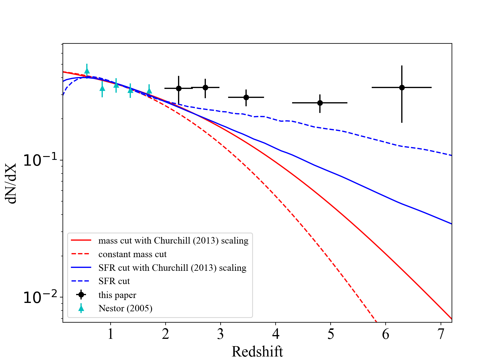
Figure 13.— Comparison of the comoving absorber number density with $W_{r}>0.3\AA$ with halo statistics from Illustris. The green triangles at low redshift are from Nestor et al. (2005), black points are from this paper. The red and blue curves correspond to integrating the dark matter halo mass function down to a fixed, redshift-independent mass or to a fixed star formation rate, respectively. The solid and dotted lines respectively denote models in which halos have 50$\%$ covering fraction out to $R=90$ proper kpc or total cross sections that scale with dark matter mass as in Churchill et al. (2013). The mass functions are taken from Torrey et al. (2014). The accounting of SFR vs halo mass are based on Behroozi et al. (2013)

While straight halo mass cuts are conceptually simple, we are not limited to this criterion. Numerous authors have investigated the density of halos as a function of both stellar mass and star formation rate (SFR). In fact for Paper I we found that $dN/dX$ was reproduced better at high redshift using weighted integrals of the luminosity function rather than the mass function. This was a purely empirical calculation, which used observed luminosity functions that required corrections for observations different redshifts, filters, and systematic survey completeness.

In Illustris, we have additional direct access to the star formation history of each simulated galaxy. Since the average SFR at fixed halo mass is larger at earlier times (Behroozi et al., 2013), we may integrate instead down to a fixed, redshift-independent SFR, which corresponds to lower dark matter halo mass at higher redshift. This achieves the desired effect of seeding smaller halos with Mg ii at early times.

The blue lines in Figure 13 show the result of this calculation for Illustris, using a constant-radius $90$ pkpc halo for objects above SFR$>0.5M_{\odot}$/yr (blue dashed line) and Churchill’s mass-dependent radial scaling for objects with SFR$>0.02M_{\odot}$/yr (solid blue line). As before the minimum SFRs are selected to fit low redshift (Nestor et al., 2005) measurements. This methodology increases $dN/dX$ by an order of magnitude or more at high redshifts, partially mitigating the discrepancy with a redshift-independent, fixed-mass bound on the integration. However there is no single value for the SFR cutoff that fits all redshifts; the value chosen here is a compromise but predicts too many Mg ii absorbers at low redshift and slightly too few at early times.

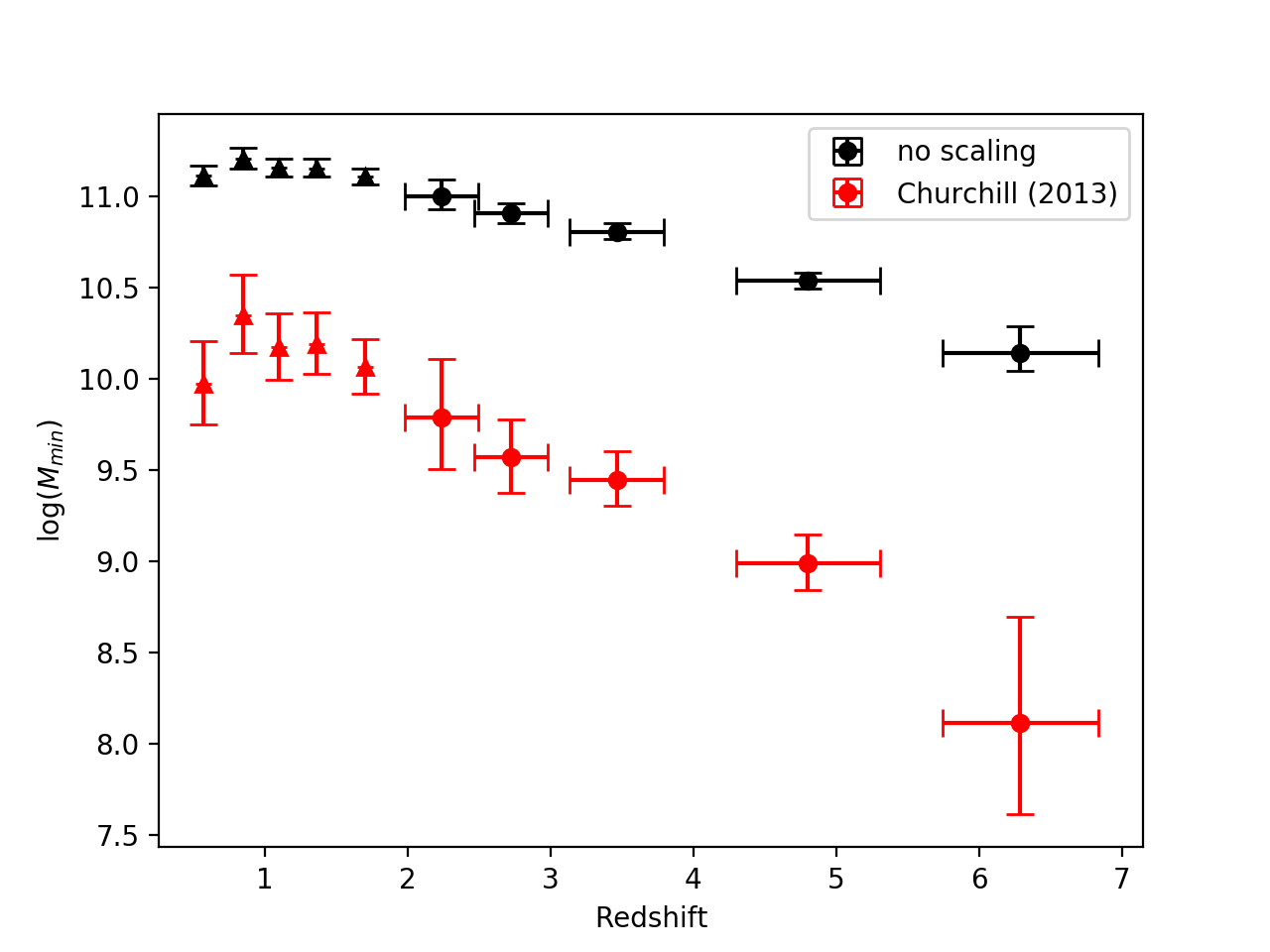
Figure 14.— Minimum dark matter halo mass cuts required to reproduce the observed comoving absorber line densities, which decline by an order of magnitude or more in our survey’s redshift range. The black and red points give the mass cut in models where halos have a fixed, $90$ kpc cross section with 50$\%$ covering fraction and where halo cross sections scale as in Churchill et al. (2013), respectively. The triangular points at lower redshifts correspond to data from Nestor et al. (2005), and the circular points derive from our data.

5.2.1 Can Low-Mass Galaxies Yield Enough Magnesium to Enrich Gaseous Halos?

At face value the small halo masses at high redshift in Figure 14—corresponding to even smaller stellar masses—require us to consider whether the these objects’ stellar populations could plausibly produce enough magnesium to fill their intra-halo media at the radii required for observation.

If we define the galaxy yield $\eta$ as the ratio of magnesium mass in the circumgalactic halo to the galaxy’s stellar mass, then for a mass-independent halo radius:

$$\eta \equiv {{M_{Mg}}\over{M_{*}}}$$

$$= \frac{1}{M_{*}}\kappa\pi R^{2}N_{{\rm Mg\;\mbox{\tiny II}}}f^{-1}m_{{\rm Mg\;\mbox{\tiny II}}}$$

$$= 2.5\times 10^{-5}\left(\frac{R}{90\text{ kpc}}\right)^{2}\left(\frac{M_{*}}{10^{10}M_{\odot}}\right)^{-1}\left(\frac{N_{{\rm Mg\;\mbox{\tiny II}}}}{10^{13}\text{ cm}^{-2}}\right)$$

$$\times\left(\frac{\kappa}{0.5}\right)\left(\frac{f}{0.1}\right)^{-1},$$

where $\kappa$ represents the Mg ii absorption covering factor, $R$ is the gaseous halo radius, $f$ is the Mg ii ionization fraction, $m_{{\rm Mg\;\mbox{\tiny II}}}=24.3u$ is the mass of a magnesium ion, and $N_{{\rm Mg\;\mbox{\tiny II}}}=10^{13}$cm^-2 represents the typical column density of a modestly saturated absorption component. For our lowest-mass halos at $z\sim 6-7$, Figure 13 provides a lower integration limit of $M_{h}\sim 10^{10.2}M_{\odot}$, corresponding to a stellar mass of $10^{8}M_{\odot}$ (Behroozi et al., 2013). For these inputs the required galactic yield of $\eta=0.0025$ is larger than the the IMF-weighted stellar magnesium yield of $\sim 0.001$ (Saitoh, 2017). Although numerical simulations do require that a significant fraction of the stellar yield is returned to the halo (Peeples et al., 2014), it is still the case that a $10^{8}M_{\odot}$ stellar population produces too little Mg ii to fill a halo to 90kpc with observable Mg ii , by a factor of a few.

This discrepancy is reduced if we invoke a larger number of lower-mass halos, with radii scaled as $R\propto M^{\gamma}$ as calculated in Figure 13. Then, the required yield becomes:

$$\eta=2.5\times 10^{-5}\left(\frac{M_{*}}{10^{10}M_{\odot}}\right)^{2\gamma-1}\left(\frac{N_{{\rm Mg\;\mbox{\tiny II}}}}{10^{13}\text{cm}^{-2}}\right)\left(\frac{\kappa}{0.5}\right)\left(\frac{f}{0.1}\right)^{-1}.$$ (11)

For $\gamma\sim 0.39$ (Churchill et al., 2013) and a $M_{*}\sim 10^{7}M_{\odot}$ stellar mass (associated with the $M_{h}\sim 10^{8}M_{\odot}$), $\eta=0.00011$, roughly an order of magnitude smaller than the IMF-weighted magnesium yield, leaving a comfortable margin to account for the difference between the strict stellar yield and the galactic yield of Mg mass ejected into the halo.

As a final, crude consistency test, we explore whether individual small halos have the correct combination of size and density to produce observable Mg ii absorption lines. For an average chord length throguh the halo of $\bar{l}=\frac{4}{3}R$, and the mass-scaled halo radius relation from above, one obtains an order-of-magnitude estimate of the column density:

$$N_{{\rm Mg\;\mbox{\tiny II}}}=4\times{10^{13}\text{ cm}^{-2}}\left(\frac{\eta}{0.001}\right)\left(\frac{f}{0.1}\right)^{-1}\left(\frac{M_{*}}{10^{7}M_{\odot}}\right)^{1-2\gamma}.$$ (12)

This column density is sufficient to produce saturated absorption, though in any realistic model of the halo one expects cool gas to be more highly structured(Crighton et al., 2015), leading to a lower covering fraction but slightly more variant total column densities in individual sightline samples.

Taken together, these results point to a modest tension for models where Mg ii is hosted at high redshift by massive galaxies with $R\sim 100$ kpc gas envelopes; in contrast models populating Mg ii in galaxies with $\sim 10-100\times$ smaller stellar mass but $3-10\times$ smaller gas envelopes comfortably accommodate the observations for reasonable heavy element yields.

Such objects would be qualitatively distinct from the $L^{*}$ galaxies hosting Mg ii in the low-redshift universe, although they could evolve over time into such massive systems. If they are not yet dynamically relaxed, it may be the case that the observed Mg ii is not solely a byproduct of winds from the halo’s internal stellar population, but rather combines winds with material stripped through interactions during the initial assembly of the halo. In this case some fraction of the heavy elements producing observed absorption may never have been in the halo center, reducing the requirements on wind transport during epochs where the Hubble time was $<1$ Gyr.

5.3. Limitations of Large-Scale Simulations for Interpreting Mg ii Observables

The statistics presented in the previous section made reference to cosmological simulations of galaxy formation (specifically the Illustris simulation) but employed a simple analytic model to predict the likelihood of absorption by a given galaxy’s CGM. This model utilizes covering fractions derived from low redshift observations to derive a binomial hit/miss rate, and has no power to predict equivalent widths or absorber kinematics (which are closely correlated).

These same simulations incorporate sophisticated hydrodynamic solvers and can therefore can be used—at least in principle—to calculate line densities and frequency distributions directly without resort to assumptions about covering fraction. Indeed, these CGM statistics can serve as an independent check on the simulations’ feedback prescriptions, beyond the present day galaxy mass function and star-formation main sequence (which the simulations reproduce by design). In practice however, computational limitations of the simulations make direct predictions of the cosmological evolution of cool gas quite difficult. In this section, we use a simple analysis of the Illustris simulation (Vogelsberger et al., 2014a; Genel et al., 2014; Sijacki et al., 2015) to demonstrate some of the challenges.

Figure 15 depicts the Mg ii absorber frequency distribuion in our $z=3.15$-$3.81$ redshift bin, along with the predicted frequency distributions found in three different runs at these redshifts used for resolution convergence testing in Illustris. The simulation boxes are $75h^{-1}$ comoving Mpc on a side, with $18.1,2.3$ and $0.3\times 10^{9}$ hydro cells and a minimum cell size of $48,98,$ and $273$ pc, respectively (Vogelsberger et al., 2014a). The simulation tracks metallicity, temperature, density, and velocity for each cell in the simulation. We calculate absorption profiles in post-processing using the methodology and code described in Bird et al. (2015). In short, the ionization balance for each cell is calculated using the UV background spectrum of Faucher-Giguère et al. (2009) at the appropriate redshift, applied to a grid of ionization fractions calculated using CLOUDY (Ferland et al., 1998). Because Mg ii has an ionization potential of 1.1 Ryd, neutral hydrogen can shield it efficiently from ionizing radiation. Since its ionization potential is very close to that of hydrogen, we make a simple correction for self-shielding of absorbing structures using the formalism of Rahmati et al. (2013). Absorbers were identified via instances where the simulated spectra dip 5 percent below continuum values. Absorption troughs within 500 km/s of each other were grouped together and identified as single absorbers. The equivalent widths of such absorbers were then calculated by integrating 500 km/s past the most extremal components of each absorber.

Figure 15 shows that the simulations produce too few Mg ii absorbers except for the weakest values of $W_{r}$. There is a marginal increase in the normalization of the predicted frequency distribution as the simulation resolution is increased. However, the slope of the simulated distribution remains steeper than the observed slope at all resolutions. Even at $W_{r}\sim 1$Å, the Universe has $3$-$10\times$ more absorbers than the simulations; at larger equivalent widths the discrepancy spans many orders of magnitude, since the box contains few or no systems at $W_{r}\gtrsim 2$Å.

The simulations’ relatively coarse mesh resolution, required to simulate a large cosmological volume, likely contributes to this deficit of strong absorbers. The spatial resolution of a single particle can be approximated as

$$l=7.1\mathrm{kpc}\left(\frac{m_{\mathrm{res}}}{10^{6}M_{\odot}}\right)^{1/3}\left(\frac{\rho}{10^{-3}\mathrm{cm}^{-3}}\right)^{-1/3}$$ (13)

where $m_{\mathrm{res}}$ is the gas mass resolution of the simulation and $\rho$ is the gas density. Even with the aggressively high particle count in the Illustris simulation, the baryon mass resolution is $m_{\mathrm{res}}=1.26\times 10^{6}M_{\odot}$ with gives an associated particle spatial resolution of $\sim$7 kpc. While the dense interstellar medium will have higher spatial resolution, the comparatively diffuse CGM can only be expected to have spatial resolution of order tens of kiloparsecs. The coarse resolution can affect predictions of absorption statistics in two important ways.

First, limited simulation spatial resolution may suppress important small scale fluctuations in density, temperature, and velocity. In the case of the CGM in Illustris-1, any density/temperature fluctuations or bulk/turbulent velocity fluctuations with spatial scales less than $\sim$10 kpc at typical CGM gas densities will not be captured. For the lower resolution Illustris-2 and Illustris-3 simulations, the CGM spatial resolution is degraded further. Indeed the higher resolution runs exhibit an increase in the overall normalization of the Mg ii frequency distribution, indicating that numerical convergence has not yet been attained in regions producing Mg ii absorption. Moving to yet higher resolution may lead to a continued increase in the overall normalization of the Mg ii frequency distribution as smaller-scale density fluctuations continue to be resolved .

Evidence for unresolved simulated CGM velocity substructure comes from the deficit of strong absorbers. In these systems, individual absorption components are saturated, so the Mg ii equivalent width is a proxy for velocity dispersion. Simple tests show that the Illustris Mg ii absorbers easily meet the column density criterion for saturation. They simply did not have enough velocity substructure to generate large equivalent widths. The existence of unresolved simulated CGM velocity substructure could easily follow from the limited spatial resolution employed in Illustris. As with density fluctuations, bulk/turbulent velocity distributions on spatial scales less than a few cell sizes (i.e. tens of kpc) are unlikely to be captured.

The second and more subtle issue concerns the position of Mg ii absorbing gas in the density-temperature plane. As a ubiquitous constituent of the CGM, Mg ii traces material in the transition range between the IGM and the ISM. To simplify and speed calculations in these regions with short cooling time scales, most numerical codes also transition somewhere in this density regime to a sub-grid physics model that will necessarily compromise some of their predictive power for studying gas physics. Figure 16 shows the phase diagram in the Temperature-density plane for Illustris, with a color scale indicating the cross-section weighted Mg ii distribution function in different parts of the plane (i.e. the fraction of all Mg ii cross section in the box contained within a bounded logarithmic interval of $n$ and $T$). More than 80% of the aggregate Mg ii cross section in Illustris resides within the contour defined by an ionization-fraction $f_{{\rm Mg\;\mbox{\tiny II}}}=0.1$. Here gas is either generally under-resolved (Equation 13) or has transitioned onto an effective equation-of-state implemented in Illustris (represented by a thin line at lower right for $n>0.13$ cm^-3).

Particles on the effective equation-of-state are modeled using a two phase medium of cool clouds embedded in a hot tenuous phase, and these particles are assigned a star formation rate and associated IMF. In practice, these cells are treated as current or future ISM constituents, and simplified in exactly the region where the phase diagram indicates that Mg ii should be strongest in the CGM.

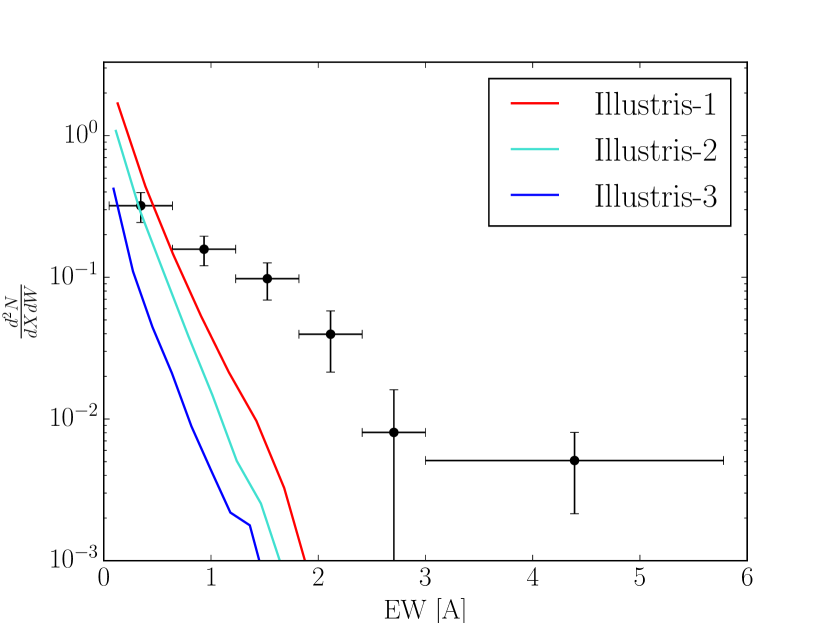
Figure 15.— Comparison of the survey equivalent width distribution (blue points) to three different runs of Illustris at redshift z = 3.5 to test resolution convergence. The simulation boxes for Illustris 1, 2, and 3 are $75h^{-1}$ comoving Mpc on a side, with $18.1,2.3$ and $0.3\times 10^{9}$ hydro cells and a minimum cell size of $48,98,$ and $273$ pc, respectively. Weaker absorbers with $W_{r}<1$Å are produced at approximately the correct rate, although the equivalent width distribution is not fully converged even at the highest resolution. Stronger absorbers are underproduced by a large factor at all resolutions.

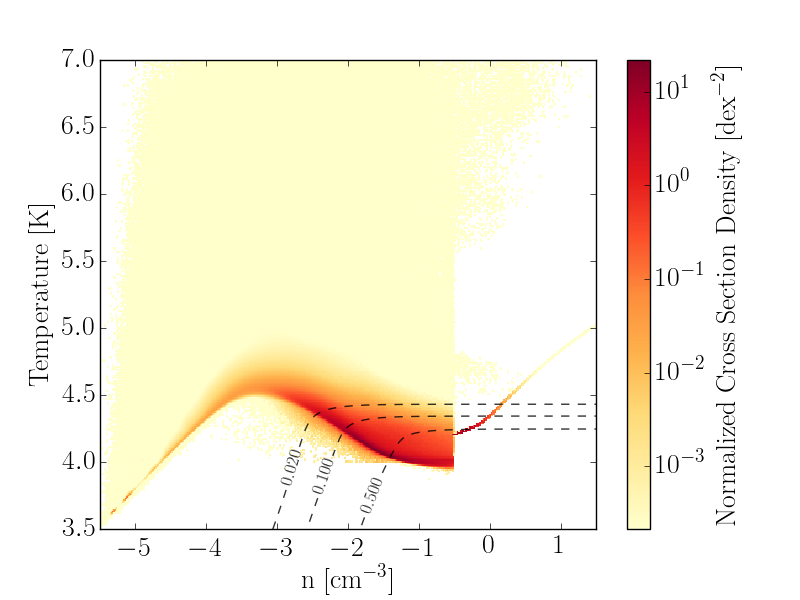
Figure 16.— Temperature-density phase diagram of illustris cells, color coded by cross-section weighted Mg ii distribution function. Dashed lines show the Mg ii ionization fraction $f_{Mg~{}{\sc ii}~{}}$. The $f_{Mg~{}{\sc ii}~{}}=0.1$ contour, roughly corresponding to temperatures below $10^{4.5}$ K and densities above $10^{-2}\text{ cm}^{-3}$, contain about 82% of the Mg ii in Illustris. Most of the Mg ii thus reside in either under-resolved regions of the simulation or on the effective equation-of-state.

These shortcomings could possibly be mitigated for the study of individual absorbers by using a galaxy scale simulation with similar resolution and/or refinement (Shen et al., 2012; Churchill et al., 2015; Muratov et al., 2015). By transitioning to sub-grid physics at smaller scales these smaller boxes track CGM gas physics with higher fidelity but are less useful for studying cosmological statistics and number counts.

As an intermediate step, we tested whether the observed equivalent width distribution could be reproduced by artificially inflating the line-of-sight velocity dispersions of Illustris Mg ii in post-processing. We find that this can be achieved by uniformly broadening the Voigt profiles of simulation particles contributing to our simulated spectra, effectively adding an additional velocity dispersion associated with unresolved bulk flows of $b\sim 40$ km s^-1(Figure 17). This procedure has no effect on the equivalent width of unsaturated profiles, but for saturated systems $W_{r}$ is increased by spreading the absorption over a wider velocity range.

The driving source for this unresolved turbulence is left unspecified. However the strongest ($W_{r}>1$Å) absorbers that most clearly reveal unresolved velocity substructure peak in incidence at $z=2$-$3$, coincident with the global star formation rate (Figure 12).

Although this prescription works for any single redshift, Illustris also predicts redshift evolution in the overall normalization of the frequency distribution, in contrast to the observations (Figure 18). Yet despite these detailed discrepancies, the simulations do produce approximately the correct total number of Mg ii absorbers—they simply allocate too many to low values of $W_{r}$. A natural interpretation is that Mg and even Mg ii is broadly being produced and distributed in a physically plausible spatial pattern within the simulation box, but is insufficiently stirred. The large-volume simulations would then provide accurate overall number counts, but smaller volumes (Joung et al., 2012; Armillotta et al., 2017; Brüggen & Scannapieco, 2016) will be the most promising avenue to resolve outstanding questions about the micro-physics of enrichment, turbulence, and the interaction of intra-halo gas with material flowing into and out of the central disk.

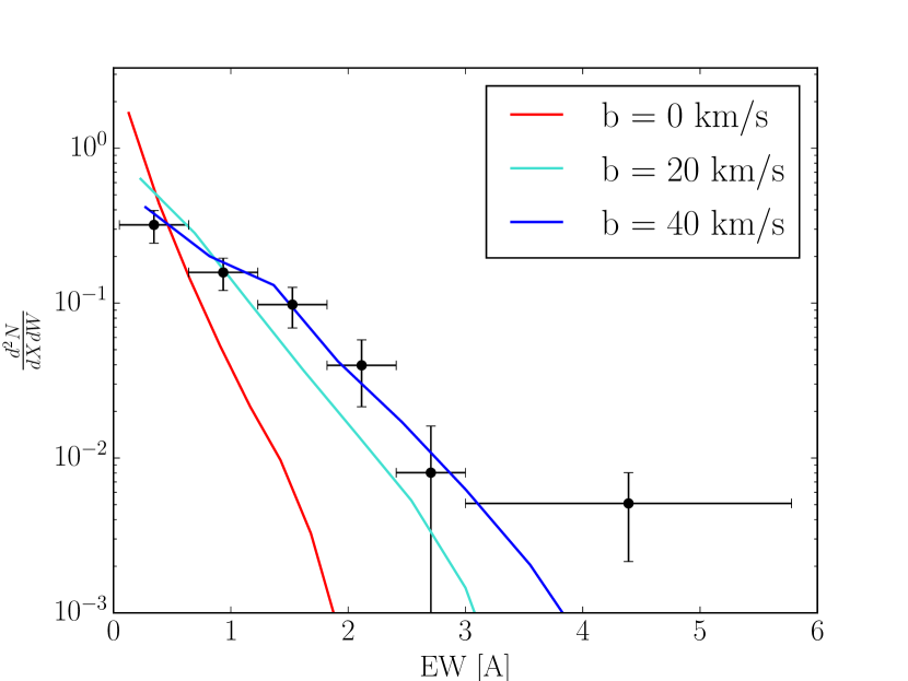
Figure 17.— Reconciliation of the equivalent width distribution determined from Illustris sightlines (solid lines) with observed data at $z=3.5$ (points with errors) by artificial inflation of the 1D bulk velocity dispersion. The paucity of strong absorbers in the un-adjusted simulation arises from unresolved velocity substructure rather than insufficient densities—the simulated densities produce saturated absorption, just over too small of a velocity interval. Artificial inflation with a $40$ km/s kernel brings the two curves into agreement.

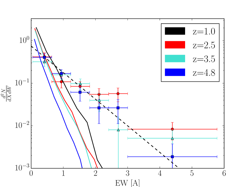
Figure 18.— Redshift evolution of the equivalent width distribution both from observations (colored points) and Illustris simulations (solid curves). At all redshifts, the simulated slope is too steep (see Figure 17). Also, there is mild evolution in the normalization of the simulated curves, in contrast to the data which evolve somewhat in slope but not in normalization.

6. conclusions

We have completed an infrared survey for Mg ii at $1.9<z<7.0$, augmenting the sample first presented in Paper I. We searched Magellan/FIRE spectra of 100 QSOs, with particular emphasis in this paper on objects at $z>6$, which provide Mg ii pathlength in the $K$ band that was not explored in previous work. This choice enables a more significant detection of evolutionary trends in the Mg ii absorber population. The reported Mg ii absorbers were identified by means of an automated finding routine and verified by eye; the completeness and false-positive rates of both automated and user-evaluated steps were then tested using a large suite of Monte Carlo simulations. Our main findings can be summarized as follows:

1. We confirm and strengthen an evolutionary decline in the frequency of strong Mg ii absorbers ($W_{r}>1$ Å) by roughly an order of magnitude in our survey’s redshift range, while the frequency of weaker absorbers remains remarkably constant from $z=0.25$-$7.0$. The Mg ii equivalent width distribution function (EWDF) slope $W_{\ast}$ does not continue its growth at low redshifts but rather peaks at $z\sim 2$-$3$, after which the incidence of strong absorbers begins to decline.

2. The inclusion of high-redshift sightlines yielded 7 systems with $z>6$. These are the first known Mg ii absorbers above this redshift, which was not covered in Paper I. Remarkably, these detections are consistent with the continued non-evolution of the weak absorbers seen at low redshifts. The single strong absorber detected at $z>6$ is also consistent with the decline of the strong absorber population, albeit with large shot noise. The persistence of the low-z population trends is also reflected in the continued decay of $W_{\ast}$ from $z=2$ onwards.

3. The peak in the frequency of strong Mg ii absorbers at $z\sim 2$ and the subsequent decline towards higher redshifts resembles the evolution of the cosmic SFR density. Our new measurements confirm the agreement between the Mg ii-to-SFR density scaling of (Ménard et al., 2011) and direct measurements of the SFR density using the Hubble Space Telescope. When this analysis is extended to include our highest redshift strong absorber, we find that the Mg ii-derived and observed SFR densities are coincident. Aforementioned cautions aside, the agreement between thus derived SFR densities suggests a connection between Mg ii absorbers and star formation.

4. Analytic calculations using Illustris-derived halo mass functions, which populate halos above a lower mass bound prescripteively with Mg ii, severely under-predict the total incidence of absorbers with $W_{r}>0.3$ Å at $z\gtrsim 2.5$. This is unsurprising given the non-evolution of the weak absorbers and the substantial evolution of the mass function in our survey’s redshift range. A simple modification wherein we populate halos above a minimum SFR cut (rather than a mass cut) achieves a redshift-dependent minimum mass. This partly alleviates the models’ deficiency of Mg ii at high redshift but remains rather imperfect.

5. Spectra computed directly by projecting sightlines through the Illustris simulation’s gas volume produce approximately the correct number of weak Mg ii absorbers but they under-predict strong Mg ii counts at all redshifts. Current cosmological simulations do not sufficiently resolve the structure of CGM gas to properly sample the density and temperature regime at which Mg ii absorption manifests. As both simulated and observed Mg ii absorbers tend to be saturated, subgrid models which merely add spatial power or increase the simulated Mg ii column density cannot reproduce the observed Mg ii absorber distribution. Because equivalent widths reflect turbulent broadening of saturated components, a successful subgrid model will need to include velocity substructure as well. We are able to qualitatively reproduce the observed Mg ii rest equivalent width distribution by assuming subgrid bulk turbulence at the $b\sim 40$ km s^-1level in Illustris; however the degree of artificial turbulence required is specific to the simulation being considered.

The continued presence of Mg ii absorption at $z=6$-$7$—even in our limited number of $z>6.3$ sightlines—suggests that the enrichment of the CGM was underway quite early, while the dark matter halos of future galaxies were still assembling and their stellar populations had yet to fully form and coalesce into pronounced disks. Indeed our highest redshift point (centered at $z=6.3$) post-dates the instantaneous reionization redshift inferred from the $\tau=0.058$ measurement of Planck (Planck Collaboration et al., 2016b) by only $240$ Myr. Given that matter moving at 100 km s^-1travels roughly 1 kpc every 10 Myr, there is scarcely enough time for a halo to accrete gas into its center, develop a stellar population, deposit feedback into the surroundings, and transport such material far enough back into the halo to produce an appreciable absorption cross section. It may be the case that early intra-halo gas is enriched by elements manufactured in accreted satellites or other in-situ star formation environments before they are subsumed into a galaxy’s central condensate. This would especially be true if early Mg ii absorbers preferentially occur in rich or highly biased environments where the earliest galaxies would have formed.

Our detection of numerous Mg ii systems at $z>6$—unlike C iv systems which decline rapidly toward higher $z$ (Simcoe et al., 2011)—is promising for future investigation of the reionization epoch using metal absorption lines. Searches for low-ionization metals in O i, Si ii, and C ii in the $J$ band have yielded some success (Becker et al., 2006), but these ions cover a smaller pathlength per QSO because they have rest wavelengths near Ly-$\alpha$. Mg ii is an abundant $\alpha$ element with large oscillator strength, has a long pathlength, is easily identified as a doublet, and can be measured out to $z\sim 8$ from the ground if suitable QSOs are identified. If so, it will be possible to study metal enrichment in CGM from nearly the current epoch ($z=0.2$) to the CMB electron scattering redshift ($z\sim 8$) using a single characteristic transition.

References

- Armillotta et al. (2017) Armillotta, L., Werk, J. K., Prochaska, J. X., Fraternali, F., & Marinacci, F. 2017, MNRAS, 470, 114
- Bañados et al. (2014) Bañados, E., Venemans, B. P., Morganson, E., et al. 2014, AJ, 148, 14
- Bañados et al. (2016) Bañados, E., Venemans, B. P., Decarli, R., et al. 2016, ApJS, 227, 11
- Bahcall & Spitzer (1969) Bahcall, J. N., & Spitzer, Jr., L. 1969, ApJ, 156, L63
- Banados (2017) Banados, E. 2017, in preperation
- Becker et al. (2011) Becker, G. D., Sargent, W. L. W., Rauch, M., & Calverley, A. P. 2011, ApJ, 735, 93
- Becker et al. (2006) Becker, G. D., Sargent, W. L. W., Rauch, M., & Simcoe, R. A. 2006, ApJ, 640, 69
- Behroozi et al. (2013) Behroozi, P. S., Wechsler, R. H., & Conroy, C. 2013, ApJ, 770, 57
- Bergeron (1986) Bergeron, J. 1986, A&A, 155, L8
- Bergeron & Boissé (1991) Bergeron, J., & Boissé, P. 1991, A&A, 243, 344
- Bird et al. (2015) Bird, S., Haehnelt, M., Neeleman, M., et al. 2015, MNRAS, 447, 1834
- Bond et al. (2001) Bond, N. A., Churchill, C. W., Charlton, J. C., & Vogt, S. S. 2001, ApJ, 562, 641
- Bordoloi et al. (2011) Bordoloi, R., Lilly, S. J., Knobel, C., et al. 2011, ApJ, 743, 10
- Bordoloi et al. (2014) Bordoloi, R., Tumlinson, J., Werk, J. K., et al. 2014, ApJ, 796, 136
- Bosman et al. (2017) Bosman, S. E. I., Becker, G. D., Haehnelt, M. G., et al. 2017, MNRAS, 470, 1919
- Bouché et al. (2007) Bouché, N., Murphy, M. T., Péroux, C., et al. 2007, ApJ, 669, L5
- Bouché et al. (2016) Bouché, N., Finley, H., Schroetter, I., et al. 2016, ApJ, 820, 121
- Brüggen & Scannapieco (2016) Brüggen, M., & Scannapieco, E. 2016, ApJ, 822, 31
- Charlton et al. (2003) Charlton, J. C., Ding, J., Zonak, S. G., et al. 2003, ApJ, 589, 111
- Chen et al. (2010) Chen, H.-W., Helsby, J. E., Gauthier, J.-R., et al. 2010, ApJ, 714, 1521
- Chen et al. (2015) Chen, Z.-F., Gu, Q.-S., & Chen, Y.-M. 2015, ApJS, 221, 32
- Churchill (2001) Churchill, C. W. 2001, ApJ, 560, 92
- Churchill et al. (2000) Churchill, C. W., Mellon, R. R., Charlton, J. C., et al. 2000, ApJS, 130, 91
- Churchill et al. (2013) Churchill, C. W., Trujillo-Gomez, S., Nielsen, N. M., & Kacprzak, G. G. 2013, ApJ, 779, 87
- Churchill et al. (2015) Churchill, C. W., Vander Vliet, J. R., Trujillo-Gomez, S., Kacprzak, G. G., & Klypin, A. 2015, ApJ, 802, 10
- Codoreanu et al. (2017) Codoreanu, A., Ryan-Weber, E. V., Crighton, N. H. M., et al. 2017, MNRAS, 472, 1023
- Crighton et al. (2015) Crighton, N. H. M., Hennawi, J. F., Simcoe, R. A., et al. 2015, MNRAS, 446, 18
- Cushing et al. (2004) Cushing, M. C., Vacca, W. D., & Rayner, J. T. 2004, PASP, 116, 362
- Dekel et al. (2009) Dekel, A., Birnboim, Y., Engel, G., et al. 2009, Nature, 457, 451
- Faucher-Giguère et al. (2009) Faucher-Giguère, C., Lidz, A., Zaldarriaga, M., & Hernquist, L. 2009, ApJ, 703, 1416
- Faucher-Giguère & Kereš (2011) Faucher-Giguère, C.-A., & Kereš, D. 2011, MNRAS, 412, L118
- Ferland et al. (1998) Ferland, G. J., Korista, K. T., Verner, D. A., et al. 1998, PASP, 110, 761
- Ford et al. (2016) Ford, A. B., Werk, J. K., Davé, R., et al. 2016, MNRAS, 459, 1745
- Fumagalli et al. (2014) Fumagalli, M., Hennawi, J. F., Prochaska, J. X., et al. 2014, ApJ, 780, 74
- Gauthier et al. (2010) Gauthier, J.-R., Chen, H.-W., & Tinker, J. L. 2010, ApJ, 716, 1263
- Genel et al. (2014) Genel, S., Vogelsberger, M., Springel, V., et al. 2014, MNRAS, 445, 175
- Jiang et al. (2016) Jiang, L., McGreer, I. D., Fan, X., et al. 2016, ApJ, 833, 222
- Joung et al. (2012) Joung, M. R., Bryan, G. L., & Putman, M. E. 2012, ApJ, 745, 148
- Kacprzak et al. (2011) Kacprzak, G. G., Churchill, C. W., Evans, J. L., Murphy, M. T., & Steidel, C. C. 2011, MNRAS, 416, 3118
- Kelson (2003) Kelson, D. D. 2003, PASP, 115, 688
- Kereš et al. (2005) Kereš, D., Katz, N., Weinberg, D. H., & Davé, R. 2005, MNRAS, 363, 2
- Kornei et al. (2012) Kornei, K. A., Shapley, A. E., Martin, C. L., et al. 2012, ApJ, 758, 135
- López & Chen (2012) López, G., & Chen, H.-W. 2012, MNRAS, 419, 3553
- Lovegrove & Simcoe (2011) Lovegrove, E., & Simcoe, R. A. 2011, ApJ, 740, 30
- Lundgren et al. (2009) Lundgren, B. F., Brunner, R. J., York, D. G., et al. 2009, ApJ, 698, 819
- Lynch & Charlton (2007) Lynch, R. S., & Charlton, J. C. 2007, ApJ, 666, 64
- Martin et al. (2012) Martin, C. L., Shapley, A. E., Coil, A. L., et al. 2012, ApJ, 760, 127
- Matejek & Simcoe (2012) Matejek, M. S., & Simcoe, R. A. 2012, ApJ, 761, 112
- Mazzucchelli (2017) Mazzucchelli, C. 2017, in preperation
- Mazzucchelli (2017, in preparation) Mazzucchelli, C. e. a. 2017, in preparation
- Ménard et al. (2011) Ménard, B., Wild, V., Nestor, D., et al. 2011, MNRAS, 417, 801
- Misawa et al. (2008) Misawa, T., Charlton, J. C., & Narayanan, A. 2008, ApJ, 679, 220
- Mortlock et al. (2011) Mortlock, D. J., Warren, S. J., Venemans, B. P., et al. 2011, Nature, 474, 616
- Muratov et al. (2015) Muratov, A. L., Kereš, D., Faucher-Giguère, C.-A., et al. 2015, MNRAS, 454, 2691
- Nestor et al. (2011) Nestor, D. B., Johnson, B. D., Wild, V., et al. 2011, MNRAS, 412, 1559
- Nestor et al. (2005) Nestor, D. B., Turnshek, D. A., & Rao, S. M. 2005, ApJ, 628, 637
- Nielsen et al. (2015) Nielsen, N. M., Churchill, C. W., Kacprzak, G. G., Murphy, M. T., & Evans, J. L. 2015, ApJ, 812, 83
- Noterdaeme et al. (2010) Noterdaeme, P., Srianand, R., & Mohan, V. 2010, MNRAS, 403, 906
- Oppenheimer et al. (2010) Oppenheimer, B. D., Davé, R., Kereš, D., et al. 2010, MNRAS, 406, 2325
- Peeples et al. (2014) Peeples, M. S., Werk, J. K., Tumlinson, J., et al. 2014, ApJ, 786, 54
- Planck Collaboration et al. (2016a) Planck Collaboration, Ade, P. A. R., Aghanim, N., et al. 2016a, A&A, 594, A13
- Planck Collaboration et al. (2016b) Planck Collaboration, Adam, R., Aghanim, N., et al. 2016b, A&A, 596, A108
- Prochaska et al. (2013) Prochaska, J. X., Hennawi, J. F., & Simcoe, R. A. 2013, ApJ, 762, L19
- Prochter et al. (2006) Prochter, G. E., Prochaska, J. X., , & Burles, S. M. 2006, The Astrophysical Journal, 639, 766. http://stacks.iop.org/0004-637X/639/766
- Quider et al. (2011) Quider, A. M., Nestor, D. B., Turnshek, D. A., et al. 2011, AJ, 141, 137
- Raghunathan et al. (2016) Raghunathan, S., Clowes, R. G., Campusano, L. E., et al. 2016, MNRAS, 463, 2640
- Rahmati et al. (2013) Rahmati, A., Pawlik, A. H., Raicevic, M., & Schaye, J. 2013, MNRAS, 430, 2427
- Rauch et al. (1999) Rauch, M., Sargent, W. L. W., & Barlow, T. A. 1999, ApJ, 515, 500
- Rauch et al. (2002) Rauch, M., Sargent, W. L. W., Barlow, T. A., & Simcoe, R. A. 2002, ApJ, 576, 45
- Rubin et al. (2012) Rubin, K. H. R., Prochaska, J. X., Koo, D. C., & Phillips, A. C. 2012, ApJ, 747, L26
- Rubin et al. (2010) Rubin, K. H. R., Weiner, B. J., Koo, D. C., et al. 2010, ApJ, 719, 1503
- Saitoh (2017) Saitoh, T. R. 2017, AJ, 153, 85
- Schneider et al. (2010) Schneider, D. P., Richards, G. T., Hall, P. B., et al. 2010, AJ, 139, 2360
- Seyffert et al. (2013) Seyffert, E. N., Cooksey, K. L., Simcoe, R. A., et al. 2013, ApJ, 779, 161
- Shen et al. (2012) Shen, S., Madau, P., Aguirre, A., et al. 2012, ApJ, 760, 50
- Sijacki et al. (2015) Sijacki, D., Vogelsberger, M., Genel, S., et al. 2015, MNRAS, 452, 575
- Simcoe et al. (2006) Simcoe, R. A., Sargent, W. L. W., Rauch, M., & Becker, G. 2006, ApJ, 637, 648
- Simcoe et al. (2011) Simcoe, R. A., Cooksey, K. L., Matejek, M., et al. 2011, ApJ, 743, 21
- Simcoe et al. (2013) Simcoe, R. A., Burgasser, A. J., Schechter, P. L., et al. 2013, PASP, 125, 270
- Steidel et al. (2002) Steidel, C. C., Kollmeier, J. A., Shapley, A. E., et al. 2002, ApJ, 570, 526
- Stern et al. (2016) Stern, J., Hennawi, J. F., Prochaska, J. X., & Werk, J. K. 2016, ApJ, 830, 87
- Storrie-Lombardi et al. (1996) Storrie-Lombardi, L. J., McMahon, R. G., Irwin, M. J., & Hazard, C. 1996, ApJ, 468, 121
- Tinker & Chen (2010a) Tinker, J. L., & Chen, H. 2010a, ApJ, 709, 1
- Tinker & Chen (2010b) Tinker, J. L., & Chen, H.-W. 2010b, ApJ, 709, 1
- Torrey et al. (2014) Torrey, P., Vogelsberger, M., Genel, S., et al. 2014, MNRAS, 438, 1985
- Torrey et al. (2015) Torrey, P., Wellons, S., Machado, F., et al. 2015, MNRAS, 454, 2770
- Tumlinson et al. (2011) Tumlinson, J., Thom, C., Werk, J. K., et al. 2011, Science, 334, 948
- Vacca et al. (2003) Vacca, W. D., Cushing, M. C., & Rayner, J. T. 2003, PASP, 115, 389
- Venemans (2017) Venemans, B. P. 2017, in preperation
- Venemans et al. (2013) Venemans, B. P., Findlay, J. R., Sutherland, W. J., et al. 2013, ApJ, 779, 24
- Venemans et al. (2015a) Venemans, B. P., Verdoes Kleijn, G. A., Mwebaze, J., et al. 2015a, MNRAS, 453, 2259
- Venemans et al. (2015b) Venemans, B. P., Bañados, E., Decarli, R., et al. 2015b, ApJ, 801, L11
- Venemans (2018, in preparation) Venemans, B. P. e. a. 2018, in preparation
- Vogelsberger et al. (2014a) Vogelsberger, M., Genel, S., Springel, V., et al. 2014a, Nature, 509, 177
- Vogelsberger et al. (2014b) —. 2014b, MNRAS, 444, 1518
- Weiner et al. (2009) Weiner, B. J., Coil, A. L., Prochaska, J. X., et al. 2009, ApJ, 692, 187
- Werk et al. (2013) Werk, J. K., Prochaska, J. X., Thom, C., et al. 2013, ApJS, 204, 17
- Willott et al. (2010) Willott, C. J., Delorme, P., Reylé, C., et al. 2010, AJ, 139, 906
- Zhu & Ménard (2013) Zhu, G., & Ménard, B. 2013, ApJ, 770, 130
- Zhu et al. (2009) Zhu, G., Moustakas, J., & Blanton, M. R. 2009, ApJ, 701, 86
- Zibetti et al. (2007) Zibetti, S., Ménard, B., Nestor, D. B., et al. 2007, ApJ, 658, 161