Ray-tracing and polarized radiative transfer in General Relativity

Abstract

We discuss the problem of polarized radiative transfer in general relativity. We present a set of equations suitable for solving the problem numerically for the case of an arbitrary space-time metric, and show numerical solutions to example problems. The solutions are computed with a new ray-tracing code, Arcmancer, developed by the authors.

1 Introduction

In curved space-times, light is observed to propagate along curved paths. As such, computing mock observations of scenes affected by strong gravity requires taking general relativity fully into account. A conceptually simple approach in the limit of geometric optics is to compute the paths of light, given by null geodesics. This can be done numerically or analytically, in the case of highly symmetric space-times such as the Kerr space-time. This approach has been often used in the literature since the late 1960’s (e.g. Cunningham & Bardeen, 1973; Luminet, 1979; Dexter, 2016). A complete solution of the polarized radiative transfer problem in curved space requires not only solving the geodesic, but solving the general relativistic polarized radiative transfer equation along this geodesic as well.

Currently, there are several codes capable of computing general relativistic polarized radiative transfer: grtrans (Dexter, 2016), Astroray (Shcherbakov & McKinney, 2013) and the code described by Broderick & Blandford (2003a, b). However, none of codes above support arbitrary space-time metrics, and are instead restricted to the Kerr metric. To remedy this, we have developed Arcmancer (Pihajoki et al. 2017, in prep): a C++ library for computing geodesics and polarized radiative transfer in space-times with arbitrary user defined metrics. In the following, we will briefly describe the general relativistic polarized radiation transfer problem and show some promising initial results.

2 Polarized radiative transfer in curved space-time

To compute radiative transfer along the path of light, given by the null geodesic $\gamma$, we need to first solve it numerically. A geodesic can be given as a curve $\gamma:\mathbb{R}\supseteq I\rightarrow M$, where $M$ is the space-time manifold, which satisfies the equations of motion. The equations of motion can be given in two complementary forms. For initial conditions $(x,k^{a})\in TM$, where $x\in M$ is the initial position and $k^{a}\in TM_{x}$ is the initial tangent vector of the geodesic, given on the tangent bundle, we have in a coordinate frame

$$\dot{x}^{\alpha} =k^{\alpha}$$ (1)

$$\dot{k}\indices =-g\indices{{}^{\alpha\beta}}\Gamma\indices{{}_{\alpha\beta\delta}}k\indices{{}^{\beta}}k\indices{{}^{\delta}}$$ (2)

$$\Gamma\indices{{}_{\alpha\beta\delta}} =\frac{1}{2}\left(\partial_{\beta}g\indices{{}_{\alpha\delta}}+\partial_{\delta}g\indices{{}_{\alpha\beta}}-\partial_{\alpha}g\indices{{}_{\beta\delta}}\right)$$ (3)

where we define $\dot{x}=\mathrm{d}x/\mathrm{d}\lambda$, and where $\lambda$ is the affine parameter of the geodesic, $g\indices{{}_{ab}}$ is the metric and $\Gamma\indices{{}_{\alpha\beta\delta}}$ are the Christoffel symbols of the first kind. For initial conditions $(x,p_{a})\in T^{*}M$, where $p_{a}\in T^{*}M_{x}$ is the initial four-momentum of the geodesic, given on the cotangent bundle, we can define a Hamiltonian $H$ and the Hamiltonian equations of motion a coordinate frame as

$$H(x,p_{a}) =\frac{1}{2}g(x)\indices{{}^{bc}}p\indices{{}_{b}}p\indices{{}_{c}}\quad\text{($=0$, for null geodesics)}$$ (4)

$$\dot{x}\indices{{}^{\alpha}} =\frac{\partial H}{\partial p\indices{{}_{\alpha}}}=g(x)\indices{{}^{\alpha\beta}}p\indices{{}_{\beta}}$$ (5)

$$\dot{p}\indices{{}_{\alpha}} =-\frac{\partial H}{\partial x\indices{{}^{\alpha}}}=-\frac{1}{2}\partial_{\alpha}g(x)\indices{{}^{\beta\delta}}p\indices{{}_{\beta}}p\indices{{}_{\delta}}.$$ (6)

The two different parametrizations are connected by the natural bijection $p\indices{{}_{a}}=g\indices{{}_{ab}}k\indices{{}^{b}}$. However, it should be noted that when plasma effects cannot be ignored, the path of light is not given by a geodesic following the dispersion relation (4), but a dispersion relation depending on the polarization and local properties of the plasma (Broderick & Blandford, 2003b). These effects are not important for the applications presented in this paper, so we can safely ignore them here.

To compute polarized radiative transfer along a geodesic, we first need to fix a polarization frame along each point of the geodesic, and connect these frames to the polarization frame at the point of observation. Conceptually the simplest method is to define a frame of two four-vectors $\{h^{a},l^{a}\}$, representing local horizontal and vertical directions, in the spatial subspace of the observer, who is assumed to move with a four-velocity $u^{a}$. If $h^{a}$ and $l^{a}$ are orthogonal with respect to each other as well as with respect to to the tangent vector of the geodesic, $k^{a}$, they define a proper polarization frame. This frame can then be parallel propagated along the geodesic to obtain a well defined polarization frame at each point of the geodesic. Next, the redshift $\mathcal{G}$ between a point on the geodesic and the observation point is given by

$$\mathcal{G}=\frac{\nu_{0}}{\nu}=\frac{{u_{0}}\indices{{}^{a}}k(x_{0})\indices{{}_{a}}}{{u}\indices{{}^{a}}k(x)\indices{{}_{a}}},$$ (7)

where $k^{a}$ is the tangent vector of the geodesic, $\nu_{0}$ and $\nu$ are the observed and emitted frequencies, $u_{0}^{a}$ and $u^{a}$ are the observer and emitter four-velocities, and $x_{0}$ and $x$ are the observation and emission points, respectively. Finally, we need a relativistic generalization of the flat space radiative transfer equation

$$\frac{\mathrm{d}\bm{\mathit{I}}_{\nu}}{\mathrm{d}s}=\bm{\mathit{J}}_{\nu}-\bm{\mathrm{M}}\,\bm{\mathit{I}}_{\nu},$$ (8)

where $s$ is the physical distance through the medium, $\bm{\mathit{I}}=(I,Q,U,V)$ is the Stokes vector, $\bm{\mathit{J}}=(j_{I},j_{Q},j_{U},j_{V})$ is the vector of corresponding emissivities and

$$\bm{\mathrm{M}}=\Biggl{(}\begin{smallmatrix}\alpha_{I}&\alpha_{Q}&\alpha_{U}&\alpha_{V}\\ \alpha_{Q}&\alpha_{I}&r_{V}&-r_{U}\\ \alpha_{U}&-r_{V}&\alpha_{I}&r_{Q}\\ \alpha_{V}&r_{U}&-r_{Q}&\alpha_{I}\end{smallmatrix}\Biggr{)}$$ (9)

is the Müller matrix containing the absorption coefficients $\alpha_{i}$ and the Faraday conversion and mixing coefficients $r_{i}$ for the various Stokes parameters. When the four-velocity of the local medium (i.e. astrophysical plasma) and a polarization reference direction $b^{a}$ (given e.g. by the local direction of the magnetic field $B$) is specified, we can use the parallel propagated polarization frame of the observer to generalize equation (8), yielding

$$\frac{\mathrm{d}\bm{\mathcal{I}}_{\nu_{0}}}{\mathrm{d}\lambda} =\bm{\mathcal{J}}_{\nu_{0}}-\bm{\mathcal{M}}_{\nu_{0}}\bm{\mathcal{I}}_{\nu_{0}}\text{, where}$$ (10)

$$\bm{\mathcal{I}}_{\nu_{0}} =\frac{\mathcal{G}^{3}}{\nu_{0}^{3}}\bm{\mathit{I}}_{\nu_{0}/\mathcal{G}},\quad\quad\bm{\mathcal{J}}_{\nu_{0}}=\frac{\mathcal{G}^{2}}{\nu_{0}^{2}}R(\chi)\bm{\mathit{J}}_{\nu_{0}/\mathcal{G}},$$ (11)

$$\bm{\mathcal{M}}_{\nu_{0}} =\frac{\mathcal{G}}{\nu_{0}}R(\chi)\bm{\mathrm{M}}_{\nu_{0}/\mathcal{G}}R(-\chi)\quad\text{and}\quad R(\chi)=\Biggl{(}\begin{smallmatrix}0&0&0&0\\ 0&\cos(2\chi)&-\sin(2\chi)&0\\ 0&\sin(2\chi)&\cos(2\chi)&0\\ 0&0&0&0\end{smallmatrix}\Biggr{)},$$ (12)

which are in general functions of frequency $\nu$, the angle $\theta$ between the four-velocity $k^{a}$ of the geodesic and the local reference direction $b^{a}$, and the angle $\chi$ between the parallel propagated polarization frame and the local reference polarization frame, projected orthogonal to $k^{a}$. See Shcherbakov & Huang (2011) for details. Given initial conditions for the intensity $\bm{\mathcal{I}}$, the emissivity $\bm{\mathit{J}}$, the response tensor $\bm{\mathrm{M}}$, the local four-velocity $u^{a}$ and the local polarization reference direction $b^{a}$ on all points of a geodesic, equation (10) can be numerically integrated along the geodesic, yielding the solution to the general relativistic polarized radiative transfer problem.

3 Example problems and future plans

The equations described above have been implemented in the Arcmancer library. Using the library we can compute results to some example problems. Figure 1 shows the comparison between numerical and analytic results to two examples of polarized radiative transfer problems in Minkowskian flat space. We see that the analytic results are well matched within the given numerical tolerance. Figure 2 shows numerically computed images of a Novikov–Thorne accretion disc (Novikov & Thorne, 1973) around a rotating Kerr black hole. The relativistic effects on the direction of the linear polarization and on the degree of polarization are clearly visible.

Our future plans are focused on testing the Arcmancer code with a larger and more demanding set of applications, such as optically thin black hole accretion flows and black hole jet synchrotron plasmas. Eventually, the full code together with the Python interface will be made freely available for the general public.

Figure 1: Comparison of a numerical (points) and an analytic (dashed lines) solution to polarized radiative transfer with constant coefficients in Minkowskian metric. Upper panel show the solutions in arbitrary units and lower panel show the residuals between numerical and analytic solutions. The panels show the solution to a problem with constant emission $\bm{\mathcal{J}}=(0,1,1,1)$ and Faraday rotation and conversion factors $r_{V}=r_{Q}=1$, with rest of the $\bm{\mathcal{M}}$ entries identically zero, starting with initial values $\bm{\mathcal{I}}=(0,0,0,0)$. $I$ is zero to within numerical precision and is not shown. For the analytic solutions, see Dexter (2016).

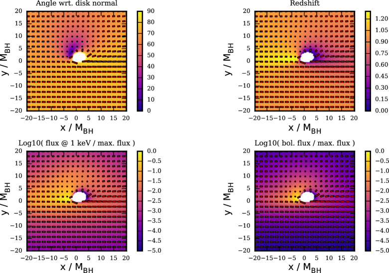
Figure 2: Ray-traced images of a Kerr black hole with a mass of $M=10\text{M}_{\odot}$, accretion rate of $\dot{M}=0.1M_{\text{Edd}}$ and a dimensionless spin of $a/M=0.998$. The surrounding accretion disc is optically thick and geometrically thin, modelled with the Novikov–Thorne equations (Novikov & Thorne, 1973). The emission is modelled with a semi-infinite electron scattering atmosphere (Chandrasekhar, 1960). The direction of linear polarization is shown by the red bars, and the degree of polarization is indicated by the bar lengths, with the degree of polarization at the bottom edges corresponding to $\sim 4\%$. Top left: The angle between the geodesic and the disc normal as measured by an observer co-moving with the disc matter. Top right: The redshift factor, $\mathcal{G}$, between the disc matter and the observation point Bottom left: Observed flux at $1\,$\mathrm{k}\mathrm{e}\mathrm{V}$$, integrated over a $10\,$\mathrm{k}\mathrm{e}\mathrm{V}$$ window, relative to the maximum flux, in logarithmic units. Bottom right: Observed bolometric flux, relative to the maximum flux, in logarithmic units.

References

- Broderick & Blandford (2003a) Broderick, A., & Blandford, R. 2003a, MNRAS, 342, 1280
- Broderick & Blandford (2003b) Broderick, A., & Blandford, R. 2003b, Ap&SS, 288, 161
- Chandrasekhar (1960) Chandrasekhar, S. 1960, Radiative transfer (Dover Publications)
- Cunningham & Bardeen (1973) Cunningham, C. T., & Bardeen, J. M. 1973, ApJ, 183, 237
- Dexter (2016) Dexter, J. 2016, MNRAS, 462, 115
- Luminet (1979) Luminet, J.-P. 1979, A&A, 75, 228
- Novikov & Thorne (1973) Novikov, I. D., & Thorne, K. S. 1973, in: C. DeWitt & B. S. DeWitt (eds.) Astrophysics of Black Holes, Black Holes (New York: Gordon and Breach), p. 343
- Shcherbakov & Huang (2011) Shcherbakov, R. V., & Huang, L. 2011, MNRAS, 410, 1052
- Shcherbakov & McKinney (2013) Shcherbakov, R. V., & McKinney, J. C. 2013, ApJ (Letters), 774, L22