Velocity Segregation and Systematic Biases In Velocity Dispersion Estimates With the SPT-GMOS Spectroscopic Survey

Matthew. B. Bayliss¹¹affiliation: Kavli Institute for Astrophysics & Space Research, Massachusetts Institute of Technology, 77 Massachusetts Ave., Cambridge, MA 02139, USA , Kyle Zengo²²affiliation: Department of Physics and Astronomy, Colby College, 5100 Mayflower Hill Dr, Waterville, ME 04901, USA , Jonathan Ruel³³affiliation: Department of Physics, Harvard University, 17 Oxford Street, Cambridge, MA 02138, USA , Bradford A. Benson⁴⁴affiliation: Department of Astronomy and Astrophysics, University of Chicago, Chicago, IL, USA 60637, USA ⁵⁵affiliation: Kavli Institute for Cosmological Physics, University of Chicago, Chicago, IL, USA 60637, USA ⁶⁶affiliation: Fermi National Accelerator Laboratory, Batavia, IL 60510-0500, USA , Lindsey E. Bleem⁵⁵affiliation: Kavli Institute for Cosmological Physics, University of Chicago, Chicago, IL, USA 60637, USA ⁷⁷affiliation: Department of Physics, University of Chicago, Chicago, IL, USA 60637, USA ⁸⁸affiliation: Argonne National Laboratory, Argonne, IL, USA 60439, USA , Sebastian Bocquet⁵⁵affiliation: Kavli Institute for Cosmological Physics, University of Chicago, Chicago, IL, USA 60637, USA ⁸⁸affiliation: Argonne National Laboratory, Argonne, IL, USA 60439, USA , Esra Bulbul¹¹affiliation: Kavli Institute for Astrophysics & Space Research, Massachusetts Institute of Technology, 77 Massachusetts Ave., Cambridge, MA 02139, USA , Mark Brodwin⁹⁹affiliation: Department of Physics and Astronomy, University of Missouri, 5110 Rockhill Road, Kansas City, MO 64110, USA , Raffaella Capasso¹⁰¹⁰affiliation: Faculty of Physics, Ludwig-Maximilians-Universität, Scheinerstr. 1, 81679 Munich, Germany ¹¹¹¹affiliation: Excellence Cluster Universe, Boltzmannstr. 2, 85748 Garching, Germany , I-non Chiu¹⁶¹⁶affiliation: Academia Sinica Institute of Astronomy and Astrophysics (ASIAA) 11F of AS/NTU Astronomy-Mathematics Building,No.1, Sec. 4, Roosevelt Rd, Taipei 10617, Taiwan , Michael McDonald¹¹affiliation: Kavli Institute for Astrophysics & Space Research, Massachusetts Institute of Technology, 77 Massachusetts Ave., Cambridge, MA 02139, USA , David Rapetti¹²¹²affiliation: Center for Astrophysics and Space Astronomy, Department of Astrophysical and Planetary Science, University of Colorado, Boulder, C0 80309, USA ¹³¹³affiliation: NASA Ames Research Center, Moffett Field, CA 94035, USA , Alex Saro¹⁰¹⁰affiliation: Faculty of Physics, Ludwig-Maximilians-Universität, Scheinerstr. 1, 81679 Munich, Germany ¹¹¹¹affiliation: Excellence Cluster Universe, Boltzmannstr. 2, 85748 Garching, Germany , Brian Stalder¹⁴¹⁴affiliation: Institute for Astronomy, the University of Hawaii, 2680 Woodlawn Dr, Honolulu, HI 96822, USA , Antony A. Stark¹⁵¹⁵affiliation: Harvard-Smithsonian Center for Astrophysics, 60 Garden Street, Cambridge, MA 02138, USA , Veronica Strazzullo¹⁰¹⁰affiliation: Faculty of Physics, Ludwig-Maximilians-Universität, Scheinerstr. 1, 81679 Munich, Germany ¹¹¹¹affiliation: Excellence Cluster Universe, Boltzmannstr. 2, 85748 Garching, Germany , Christopher W. Stubbs³³affiliation: Department of Physics, Harvard University, 17 Oxford Street, Cambridge, MA 02138, USA ¹⁵¹⁵affiliation: Harvard-Smithsonian Center for Astrophysics, 60 Garden Street, Cambridge, MA 02138, USA , Alfredo Zenteno¹⁷¹⁷affiliation: Cerro Tololo Inter-American Observatory, Casilla 603, La Serena, Chile mbayliss@mit.edu

Abstract

The velocity distribution of galaxies in clusters is not universal; rather, galaxies are segregated according to their spectral type and relative luminosity. We examine the velocity distributions of different populations of galaxies within 89 Sunyaev Zel’dovich (SZ) selected galaxy clusters spanning $0.28<z<1.08$ . Our sample is primarily draw from the SPT-GMOS spectroscopic survey, supplemented by additional published spectroscopy, resulting in a final spectroscopic sample of 4148 galaxy spectra—2868 cluster members. The velocity dispersion of star-forming cluster galaxies is $17\pm 4$ % greater than that of passive cluster galaxies, and the velocity dispersion of bright ( $m<m^{*}-0.5$ ) cluster galaxies is $11\pm 4$ % lower than the velocity dispersion of our total member population. We find good agreement with simulations regarding the shape of the relationship between the measured velocity dispersion and the fraction of passive vs. star-forming galaxies used to measure it, but we find a small offset between this relationship as measured in data and simulations in which suggests that our dispersions are systematically low by as much as 3% relative to simulations. We argue that this offset could be interpreted as a measurement of the effective velocity bias that describes the ratio of our observed velocity dispersions and the intrinsic velocity dispersion of dark matter particles in a published simulation result. Measuring velocity bias in this way suggests that large spectroscopic surveys can improve dispersion-based mass-observable scaling relations for cosmology even in the face of velocity biases, by quantifying and ultimately calibrating them out.

Galaxies: clusters: general — galaxies: distances and redshifts — galaxies: kinematics and dynamics — cosmology: observations — galaxies: evolution

1 Introduction

Spectroscopic surveys of massive galaxy clusters—the most massive gravitationally bound structures in the universe—provide important constraints on cosmological measurements of the growth of structure and valuable insights into the properties of galaxy populations in the most extreme over-dense environments. There is a long and rich history of studies using the widths of the peculiar velocity distribution of clusters, i.e., their velocity dispersions, to estimate the depths of their gravitational potential wells and infer the total masses of those clusters (Zwicky, 1937; Bahcall, 1981; Kent & Gunn, 1982; Bahcall et al., 1991; Biviano et al., 1993; Girardi et al., 1993, 1996; Dressler et al., 1999; Rines et al., 2003; Geller et al., 2013; Rines et al., 2013; Sifón et al., 2013; Ruel et al., 2014; Sifón et al., 2016). Velocity dispersion measurements are one of several mass-observable proxies that can contribute to calibrating mass measurements of clusters, which remains a prime concern for extracting competitive cosmological constraints from galaxy cluster abundance measurements (Majumdar & Mohr, 2003, 2004; Rozo et al., 2010; Allen et al., 2011; Williamson et al., 2011; Benson et al., 2013; Planck Collaboration et al., 2013; von der Linden et al., 2014; Bocquet et al., 2015; de Haan et al., 2016).

It is also well-established that the phase space properties of galaxies within clusters are not uniform across all galaxy types. For example, numerous studies have observed differences in the spatial distribution of different types of galaxies, with red/early-type/passive galaxies preferentially occupying more central radial regions of clusters while blue/late-type/star-forming galaxies are more likely to reside at larger radii (Melnick & Sargent, 1977; Dressler, 1980; Whitmore et al., 1993; Abraham et al., 1996; Balogh et al., 1997; Dressler et al., 1999; Balogh et al., 2000; Domínguez et al., 2001; Gerken et al., 2004; Rosati et al., 2014), at least at $z<1$ (Brodwin et al., 2013), and with the caveat that SZ-based cluster centroids can be significant, especially at $z>1$ (Song et al., 2012).

A similar effect is expected to occur in line-of-sight velocity space where the distribution of peculiar velocities of cluster galaxies are segregated by galaxy type. These velocity segregation effects are more challenging to measure than their spatial counterparts, but differences in the peculiar velocity distributions of different types of galaxies have been previously noted in studies. Most studies have found that blue/late-type/star-forming galaxies tend to have larger peculiar velocities than red/early-type/passive galaxies (Sodre et al., 1989; Zabludoff & Franx, 1993; Colless & Dunn, 1996; Biviano et al., 1997; Carlberg et al., 1997b; Dressler et al., 1999; Biviano et al., 2002; Ribeiro et al., 2010; Girardi et al., 2015; Barsanti et al., 2016; Biviano et al., 2016), while a few have detected evidence for more luminous cluster galaxies having systematically lower peculiar velocities than fainter cluster galaxies (Chincarini & Rood, 1977; Biviano et al., 1992; Mohr et al., 1996; Goto, 2005; Ribeiro et al., 2010; Old et al., 2013; Barsanti et al., 2016). Some studies, however, have detected no significant velocity segregation in galaxy cluster samples (Tammann, 1972; Moss & Dickens, 1977; Rines et al., 2003; Biviano & Poggianti, 2009; Rines et al., 2013; Crawford et al., 2014), suggesting the need for more analyses of larger datasets. In recent work on this topic Barsanti et al. (2016) argue specifically for the importance of analyzing large spectroscopic datasets as stacks or ensembles in order to tease out velocity segregation effects. Analyses of large ensemble datasets are ideal for revealing the average velocity segregation effects associated with sub-populations of cluster member galaxies.

Refer to caption — Figure 1: The redshift distribution and SZ-derived masses of the galaxy clusters used in this work, all SZ-selected. Masses are taken from Bleem et al. (2015) and Hasselfield et al. (2013).

In this work we present an analysis of a large sample of spectroscopically observed galaxies in 89 clusters that were selected via the Sunyaev Zel’dovich effect (SZ effect; Sunyaev & Zel’dovich, 1972, 1980). Most of these clusters are from the South Pole Telescope (SPT) SZ survey (Staniszewski et al., 2009; Vanderlinde et al., 2010; Carlstrom et al., 2011; Williamson et al., 2011; Reichardt et al., 2013; Bleem et al., 2015), with additional clusters drawn from the Atacama Cosmology Telescope (ACT) SZ survey (Marriage et al., 2011; Hasselfield et al., 2013). SPT and ACT have both performed surveys optimized ( $\sim$ 1^′ beams) for identifying galaxy clusters above approximately flat mass thresholds at $z\gtrsim 0.25$ .

Our objective is to test for the presence of systematic biases that affect velocity dispersion estimates as a function of the properties of the galaxies used to estimate those dispersions. Recent simulations provide theoretical expectations for the scaling relation between galaxy cluster mass and the observed line-of-sight velocity dispersion (Evrard et al., 2008; White et al., 2010; Diemer et al., 2013; Munari et al., 2013), but there is still a significant leap that must be made to robustly connect the dark matter particle dispersions that are easily measurable in simulations to the galaxy velocity dispersion that we actually observe (Gifford et al., 2013; Saro et al., 2013; Hernández-Fernández et al., 2014; Sifón et al., 2016). In this paper we aim to quantify velocity segregation effects in a uniformly selected sample of massive galaxy clusters, and to compare our results to recent efforts to calibrate for these effects in simulations. Quantifying the degree to which velocity segregation effects induce systematic biases in velocity dispersions estimates would provide valuable input for calibrating mass-observable scaling relations in cosmological analyses of galaxy cluster samples that utilize velocity dispersion measurements (Borgani et al., 1997).

This paper is organized into the following sections: in § 2 we describe the dataset used in our analysis, including new spectroscopy as well as spectra taken from the literature. In § 3 we describe the process that we use to generate an ensemble cluster galaxy velocity sample, and we then use that ensemble to measure velocity segregation as a function of spectral type and relative luminosity. In § 4 we compare our velocity segregation measurements to similar measurements in simulated galaxy clusters to recover estimates of the systematic biases between velocity dispersions measured in real data vs simulations. In § 5 we discuss the results of our analysis and explore the possible implications. Finally, in § 6 we summarize our results and conclusions. Unless explicitly stated otherwise, the uncertainties that we report reflect 68% confidence intervals. All magnitude measurements throughout this paper are in the AB system, and for all cosmological computations we assume a flat cosmology with $\Omega_{M}=0.3$ and $\Omega_{\Lambda}=0.7$ , $H_{0}=70$ km s^-1 Mpc^-1, and $h=H_{0}/100=0.7$ .

Table 1: Example Catalog Data for Individual Galaxies

Cluster	Object	RA	Dec	z ( $\delta_{z}$ )^a^aThe measured redshift with the uncertainty in the last two digits given in parentheses.	$W_{0}$ [O II]	$W_{0}$ H- $\delta$	$r$	$i$
Name	Name	(^∘)	(^∘)		(Å)	(Å)	(AB)	(AB)
SPT-CLJ2337-5942	J233729.84-594159.0	354.37433	-59.69973	$0.77910(32)$	$4.50\pm 2.42$	$3.51\pm 1.62$	22.63	21.31
SPT-CLJ2337-5942	J233732.53-594305.9	354.38556	-59.71831	$0.77370(29)$	$-1.16\pm 3.93$	$5.62\pm 2.23$	22.47	21.39
SPT-CLJ2337-5942	J233722.38-594318.3	354.34326	-59.72176	$0.77110(44)$	$6.85\pm 4.30$	$-0.38\pm 2.77$	22.63	21.25
SPT-CLJ2337-5942	J233718.74-594215.5	354.32806	-59.70430	$0.78330(33)$	$5.43\pm 4.08$	$1.33\pm 2.72$	23.10	21.83
SPT-CLJ2337-5942	J233729.45-594257.2	354.37271	-59.71588	$0.77590(27)$	$-0.59\pm 4.41$	$1.02\pm 2.58$	21.86	20.68
SPT-CLJ2337-5942	J233725.66-594157.9	354.35690	-59.69942	$0.77550(30)$	$-0.02\pm 3.78$	$5.54\pm 2.14$	22.39	21.12
SPT-CLJ2337-5942	J233727.50-594234.7	354.36456	-59.70963	$0.77760(24)$	$3.60\pm 2.65$	$3.37\pm 1.65$	21.09	20.10
SPT-CLJ2337-5942	J233724.13-594240.6	354.35052	-59.71128	$0.78360(41)$	$2.26\pm 5.74$	$2.55\pm 3.88$	23.40	22.04
SPT-CLJ2337-5942	J233734.02-594231.9	354.39175	-59.70886	$0.77630(37)$	$-2.27\pm 5.45$	$-1.82\pm 3.09$	22.96	21.76
SPT-CLJ2337-5942	J233738.77-594312.1	354.41156	-59.72004	$0.77480(55)$	$-4.57\pm 12.78$	$7.59\pm 6.92$	24.52	23.08

2 Spectroscopic Data and Galaxy Catalogs

2.1 SPT-GMOS and Supplemental Literature Spectroscopy

The majority of the dataset used in this analysis comes from the SPT-GMOS spectroscopic survey (Bayliss et al., 2016), which consists of spectroscopic follow-up of 62 galaxy clusters from the SPT-SZ survey. The full SPT-GMOS sample includes 2243 galaxy spectra, 1579 of which are cluster member galaxies. In addition to primary catalog information such as redshifts and positions of individual galaxies with spectra, the SPT-GMOS dataset also includes spectral index measurements made using the 1-dimensional (1D) spectrum of each individual galaxy. Where possible we supplement the SPT-GMOS spectroscopic sample with other published spectroscopy of SPT and ACT SZ-selected galaxy clusters (Brodwin et al., 2010; Sifón et al., 2013; Stalder et al., 2013; Bayliss et al., 2014; Ruel et al., 2014; Sifón et al., 2016).

Including spectroscopy from the literature in our analysis requires access to catalog information—i.e., redshifts, positions—as well as the extracted 1D spectra for individual galaxies from which we measure specific spectral index values as the strength of specific spectral features. These spectral index measurements provide significant added value to the resulting galaxy spectroscopy catalog; see § 2.4 below for a description of the spectral index measurements and the galaxy classification metrics that we use. In total we incorporate literature spectra for an additional 27 galaxy clusters, adding 1431 galaxies and 1118 cluster member galaxies for which we have access to both catalogs and the extracted spectra.

Table 2: SZ-Selected Spectroscopic Cluster Sample

Cluster Name	N_spec	N_members	N_pass+PSB	N_star-forming	${\bar{z}_{\mathrm{cluster}}}$	$\sigma_{\mathrm{v}}$	Reference(s)^a^a References: 1=Bayliss et al. (2016), 2=Ruel et al. (2014), 3=Sifón et al. (2013) 4=this work.
						(km s^-1)
SPT-CLJ0000-5748	97	56	48	8	$0.7004\pm 0.0011$	$682\pm 108$	2, 4
SPT-CLJ0013-4906	45	41	32	9	$0.4075\pm 0.0009$	$1103\pm 136$	1
SPT-CLJ0014-4952	41	29	25	4	$0.7520\pm 0.0009$	$990\pm 119$	2
SPT-CLJ0033-6326	37	18	13	5	$0.5990\pm 0.0023$	$1916\pm 292$	1
SPT-CLJ0037-5047	51	19	7	12	$1.0263\pm 0.0012$	$1350\pm 182$	2
SPT-CLJ0040-4407	44	36	30	6	$0.3498\pm 0.0010$	$1259\pm 149$	1, 2
SPT-CLJ0102-4603	44	20	15	5	$0.8405\pm 0.0014$	$808\pm 134$	1
SPT-CLJ0106-5943	44	29	19	10	$0.3484\pm 0.0011$	$1297\pm 197$	1
SPT-CLJ0118-5156	23	14	6	8	$0.7051\pm 0.0017$	$934\pm 186$	1, 2
SPT-CLJ0123-4821	29	20	16	4	$0.6550\pm 0.0018$	$1505\pm 276$	1
SPT-CLJ0142-5032	39	31	18	13	$0.6793\pm 0.0012$	$1000\pm 110$	1
SPT-CLJ0200-4852	54	35	26	9	$0.4992\pm 0.0007$	$1146\pm 97$	1
SPT-CLJ0205-6432	24	15	10	5	$0.7436\pm 0.0008$	$980\pm 203$	1, 2
SPT-CLJ0212-4657	36	26	14	12	$0.6535\pm 0.0013$	$931\pm 116$	1
ACT-CLJ0215-5212	63	54	29	25	$0.4799\pm 0.0008$	$1043\pm 97$	3
ACT-CLJ0232-5257	80	57	47	10	$0.5562\pm 0.0006$	$1020\pm 87$	3
SPT-CLJ0233-5819	11	10	8	2	$0.6637\pm 0.0015$	$754\pm 183$	1, 2
SPT-CLJ0234-5831	29	21	19	2	$0.4150\pm 0.0009$	$944\pm 155$	2
ACT-CLJ0235-5121	98	78	71	7	$0.2776\pm 0.0006$	$1095\pm 86$	3
ACT-CLJ0237-4939	68	62	55	7	$0.3343\pm 0.0007$	$1261\pm 93$	3
SPT-CLJ0243-4833	43	39	26	13	$0.4984\pm 0.0012$	$1293\pm 165$	1
SPT-CLJ0243-5930	38	26	21	5	$0.6345\pm 0.0011$	$1155\pm 135$	1, 2
SPT-CLJ0245-5302^b^b Also discovered independently by ACT (Hasselfield et al., 2013).	38	29	27	2	$0.3000\pm 0.0010$	$1262\pm 195$	1
SPT-CLJ0252-4824	33	24	17	7	$0.4207\pm 0.0006$	$882\pm 65$	1
SPT-CLJ0254-5857	42	32	25	7	$0.4377\pm 0.0015$	$1446\pm 179$	2
SPT-CLJ0304-4401	46	35	32	3	$0.4584\pm 0.0009$	$1115\pm 117$	1
ACT-CLJ0304-4921	84	70	64	6	$0.3920\pm 0.0006$	$1051\pm 83$	3
SPT-CLJ0307-6225	35	20	10	10	$0.5801\pm 0.0008$	$652\pm 153$	1
SPT-CLJ0310-4647	38	28	26	2	$0.7067\pm 0.0008$	$617\pm 72$	1
SPT-CLJ0324-6236	22	10	8	2	$0.7498\pm 0.0009$	$1358\pm 187$	1
ACT-CLJ0330-5227	81	68	62	6	$0.4417\pm 0.0008$	$1244\pm 97$	3
SPT-CLJ0334-4659	51	34	20	14	$0.4861\pm 0.0014$	$1223\pm 159$	1
ACT-CLJ0346-5438	92	86	66	20	$0.5298\pm 0.0006$	$1052\pm 105$	3
SPT-CLJ0348-4515	39	27	22	5	$0.3592\pm 0.0013$	$1246\pm 167$	1
SPT-CLJ0352-5647	29	17	16	1	$0.6490\pm 0.0016$	$813\pm 133$	1
SPT-CLJ0356-5337	36	8	4	4	$1.0359\pm 0.0042$	$1647\pm 514$	1
SPT-CLJ0403-5719	43	29	21	8	$0.4670\pm 0.0010$	$990\pm 110$	1
SPT-CLJ0406-4805	30	27	17	10	$0.7355\pm 0.0018$	$1216\pm 135$	1
SPT-CLJ0411-4819	54	44	35	5	$0.4241\pm 0.0010$	$1267\pm 113$	1
SPT-CLJ0417-4748	44	32	21	11	$0.5794\pm 0.0012$	$1133\pm 133$	1
SPT-CLJ0426-5455	17	11	7	4	$0.6420\pm 0.0017$	$910\pm 201$	1
SPT-CLJ0438-5419^b^b Also discovered independently by ACT (Hasselfield et al., 2013).	86	73	63	10	$0.4224\pm 0.0007$	$1321\pm 98$	1, 2, 3
SPT-CLJ0456-5116	40	23	19	4	$0.5619\pm 0.0007$	$822\pm 149$	1
SPT-CLJ0509-5342^b^b Also discovered independently by ACT (Hasselfield et al., 2013).	24	18	17	1	$0.4620\pm 0.0008$	$690\pm 95$	2
SPT-CLJ0511-5154	23	15	15	0	$0.6447\pm 0.0014$	$758\pm 137$	1, 2
SPT-CLJ0516-5430^b^b Also discovered independently by ACT (Hasselfield et al., 2013).	405	169	152	15	$0.2947\pm 0.0003$	$939\pm 56$	2, 4
SPT-CLJ0528-5300^b^b Also discovered independently by ACT (Hasselfield et al., 2013).	31	20	19	1	$0.7694\pm 0.0017$	$1435\pm 217$	2
SPT-CLJ0539-5744	30	19	15	4	$0.7597\pm 0.0021$	$1075\pm 140$	1
SPT-CLJ0542-4100	38	31	25	6	$0.6399\pm 0.0009$	$1032\pm 141$	1
SPT-CLJ0549-6205	35	27	24	3	$0.3755\pm 0.0006$	$666\pm 104$	1
SPT-CLJ0551-5709	41	32	21	11	$0.4243\pm 0.0007$	$871\pm 120$	2
SPT-CLJ0555-6406	39	31	23	8	$0.3455\pm 0.0008$	$1088\pm 159$	1
SPT-CLJ0559-5249^b^b Also discovered independently by ACT (Hasselfield et al., 2013).	41	37	35	2	$0.6091\pm 0.0011$	$1128\pm 141$	2
ACT-CLJ0616-5227	20	16	13	3	$0.6835\pm 0.0016$	$1104\pm 160$	3
SPT-CLJ0655-5234	34	30	25	5	$0.4724\pm 0.0009$	$883\pm 103$	1
ACT-CLJ0707-5522	64	58	48	10	$0.2962\pm 0.0006$	$826\pm 79$	3
SPT-CLJ2017-6258	43	37	34	3	$0.5354\pm 0.0009$	$972\pm 134$	1
SPT-CLJ2020-6314	28	18	11	7	$0.5367\pm 0.0013$	$891\pm 135$	1
SPT-CLJ2026-4513	25	19	14	5	$0.6887\pm 0.0017$	$1429\pm 155$	1
SPT-CLJ2030-5638	52	39	28	11	$0.3937\pm 0.0005$	$620\pm 66$	1
SPT-CLJ2035-5251	46	32	26	6	$0.5287\pm 0.0011$	$1015\pm 111$	1
SPT-CLJ2043-5035	36	21	20	1	$0.7234\pm 0.0007$	$591\pm 71$	2
SPT-CLJ2058-5608	16	9	7	2	$0.6065\pm 0.0019$	$1038\pm 357$	1, 2
SPT-CLJ2100-4548	41	20	14	6	$0.7122\pm 0.0010$	$866\pm 171$	2
SPT-CLJ2104-5224	36	22	16	6	$0.7997\pm 0.0025$	$1244\pm 172$	2
SPT-CLJ2115-4659	37	29	26	3	$0.2988\pm 0.0008$	$934\pm 128$	1
SPT-CLJ2118-5055	57	33	24	9	$0.6244\pm 0.0010$	$989\pm 108$	1, 2
SPT-CLJ2136-4704	28	24	19	5	$0.4242\pm 0.0017$	$1448\pm 224$	1, 2
SPT-CLJ2140-5727	33	17	10	7	$0.4043\pm 0.0012$	$1192\pm 282$	1
SPT-CLJ2146-4846	29	26	23	3	$0.6230\pm 0.0008$	$768\pm 103$	1, 2
SPT-CLJ2146-5736	41	25	19	6	$0.6025\pm 0.0012$	$936\pm 131$	1
SPT-CLJ2155-6048	31	24	18	6	$0.5389\pm 0.0011$	$1049\pm 145$	1, 2
SPT-CLJ2159-6244	48	41	34	7	$0.3915\pm 0.0005$	$794\pm 88$	1
SPT-CLJ2218-4519	22	20	15	5	$0.6365\pm 0.0017$	$1172\pm 143$	1
SPT-CLJ2222-4834	38	27	23	4	$0.6519\pm 0.0014$	$1002\pm 108$	1
SPT-CLJ2232-5959	38	26	23	3	$0.5948\pm 0.0010$	$1004\pm 158$	1
SPT-CLJ2233-5339	42	31	25	6	$0.4398\pm 0.0006$	$1045\pm 219$	1
SPT-CLJ2245-6206	28	4	4	0	$0.5856\pm 0.0031$	$1363\pm 953$	1
SPT-CLJ2258-4044	38	27	22	5	$0.8971\pm 0.0017$	$1220\pm 145$	1
SPT-CLJ2301-4023	49	20	17	3	$0.8349\pm 0.0023$	$1270\pm 95$	1
SPT-CLJ2306-6505	49	43	39	4	$0.5297\pm 0.0008$	$1132\pm 113$	1
SPT-CLJ2325-4111	48	33	26	7	$0.3570\pm 0.0016$	$1618\pm 275$	1, 2
SPT-CLJ2331-5051	92	82	26	39	$0.5744\pm 0.0008$	$1282\pm 100$	2
SPT-CLJ2335-4544	42	35	27	8	$0.5473\pm 0.0010$	$973\pm 126$	1
SPT-CLJ2337-5942	80	39	35	4	$0.7768\pm 0.0009$	$839\pm 105$	2, 4
SPT-CLJ2341-5119	23	14	13	1	$1.0024\pm 0.0012$	$1146\pm 233$	2
SPT-CLJ2342-5411	16	11	5	6	$1.0758\pm 0.0032$	$1253\pm 337$	2
SPT-CLJ2344-4243	42	32	25	7	$0.5953\pm 0.0018$	$1814\pm 219$	1, 2
SPT-CLJ2359-5009	29	22	13	9	$0.7749\pm 0.0011$	$912\pm 151$	2

Note. — A summary of the results of SPT-GMOS spectroscopy by galaxy cluster. Columns from left to right report (1) the cluster name, (2) the total number of galaxy spectra with redshift measurements, (3) the number of cluster member galaxies, (4) the number of passive and post-starburst members, (5) the number of star-forming members, (6) the median cluster redshift, (7) the velocity dispersion estimates for each cluster, and (8) the reference(s) for the published galaxy spectroscopy used in our analysis.

2.2 New Magellan/IMACS Spectroscopy

In addition to previously published galaxy spectroscopy, we also present the first publication of new spectroscopy in the fields of three SPT galaxy clusters. We observed SPT-CLJ0000-5748, SPT-CLJ0516-5430, and SPT-CLJ2337-5942 with the Inamori Magellan Areal Camera and Spectrograph (IMACS; Dressler et al., 2006) mounted on the Magellan-I (Baade) telescope at Las Campanas Observatory on the nights of 14-15 September 2012. SPT-CLJ0000-5748 and SPT-CLJ2337-5942 were each observed with one mult-slit mask, and SPT-CLJ0516-5430 was observed with two different multi-slit masks. All masks were observed using the IMACS f/2 (short) camera and designed to have 1.0^′′ by 6.0^′′ slitlets placed using the same color-based prioritization methodology described in numerous previous publications (Section 2.3.4 in Bayliss et al., 2016).

For the two SPT-CLJ0516-5430 mask observations IMACS was configured with the WBP4791-6397 filter and the 300 l/mm grism, resulting in individual galaxy spectra over a wavelength range of $\Delta\lambda\sim 4800-6400$ Å, with spectral dispersion of 1.34Å per pixel, a spectral resolution element of 6.7Å, and spectral resolution, $R\simeq 700-1000$ . SPT-CLJ0000-5748 and SPT-CLJ2337-5942 were observed with IMACS configured to use the WBP 6296-8053 filter and the 300 l/mm grism, resulting in individual galaxy spectra over a wavelength range of $\Delta\lambda\sim 6300-8100\AA$ , with spectral dispersion of 1.34Å per pixel, a spectral resolution element of 6.7Å, and spectral resolution, $R\simeq 900-1200$ .

We reduced and extracted the raw spectroscopic data using the COSMOS¹¹1http://code.obs.carnegiescience.edu/cosmos package (Kelson, 2003) in combination with custom IDL scripts based on the XIDL library²²2http://www.ucolick.org/~xavier/IDL/. The wavelength calibration was achieved using HeNeAr arc lamp exposures taken on-sky bracketing the science exposures, and we applied a flux calibration based on an observation of the spectrophotometric standard star LTT1788 (Hamuy et al., 1992) in the same instrument configurations as the science observations. Because we had a single epoch standard star observation we have only corrected for the wavelength-dependent response of the telescope $+$ instrument system, rather than an absolute spectrophotometric flux calibration.

We measured redshifts for the IMACS spectra by cross-correlation with the fabtemp97 and habtemp90 templates in the RVSAO package for IRAF (Kurtz & Mink, 1998). All redshifts were corroborated by visually confirming the presence of strong features by eye. Following previous work we note that the redshift uncertainties output by RVSAO underestimate the true statistical uncertainty by a factor of $\sim$ 1.7 (Quintana et al., 2000), and so we have corrected the RVSAO outputs by multiplying the uncertainties by this factor. We show a representative portion of the catalog measurements made from these new IMACS spectra in Table 1, and the full catalog of new IMACS data will be publicly released in parallel with this paper. From these IMACS data we have added 474 new galaxy spectra, 172 of which are cluster members. The inclusion of the new IMACS spectra described above and these literature data have grown the number of cluster member spectra in our raw sample by $\sim$ 80%. The full cluster dataset is described in Table 2, and all 89 clusters are plotted as a function of SZ mass and redshift in Figure 1. The full SPT-GMOS $+$ literature sample consists of 4148 galaxies, 2868 of which are cluster members.

2.3 Selecting Cluster Member Galaxies

Previous studies have rightly noted that member selection is a critical step in assembling large samples of cluster galaxies with which to test for velocity segregation effects (Biviano et al., 2006; Biviano & Poggianti, 2009; Saro et al., 2013; Girardi et al., 2015; Barsanti et al., 2016). Member selection must be treated thoughtfully in order to minimize potential biases in the dispersion estimates that could arise by including, for example, large numbers of interloper galaxies. We apply a two-stage member selection process designed to emulate the “peak $+$ gap” procedure that has been used in many previous studies (Fadda et al., 1996; Biviano et al., 2013; Girardi et al., 2015; Barsanti et al., 2016). This procedure relies on a first stage selection that takes place solely in line-of-sight velocity space, identifying velocity distributions associated with clusters as over-densities in the available radial velocity catalogs. We iteratively compute the bi-weight estimates of the center and width (i.e., median redshift and velocity dispersion) of the velocity distribution associated with each cluster in the same way as described in Bayliss et al. (2016). Briefly, we iteratively applied the bi-weight location and scale estimators from Beers et al. (1990), rejecting $>3\sigma$ outliers until converging on a stable velocity dispersion.

We then take the results of the first stage selection as a starting point and apply the “shifting gapper” procedure to select member galaxies for each cluster. The shifting gapper uses both radial velocity and projected radial information to iteratively include or reject galaxies as cluster members until convergence is reached. The shifting gapper is applied by iteratively testing each candidate member galaxy using other candidate member galaxies that are nearby neighbors in projected radius, flagging the tested galaxy as a cluster member if the largest gap in peculiar velocity among the neighbor galaxies does not exceed some fixed value. Specifically, we apply the same implementation of the shifting gapper technique as described by Crawford et al. (2014), which differs slightly from the original Fadda et al. (1996) implementation in that it uses absolute peculiar velocities rather than the raw velocity values to reflect the fact that on average, galaxy clusters are radially symmetric in velocity space (Kasun & Evrard, 2005). Our implementation also uses running bins of the nearest $n$ galaxies in radius rather than rigid radial bins (e.g., fixed $\Delta r=0.4$ or 0.5 Mpc h^-1) to avoid the effects of artificial discontinuities across bins in sparsely sampled clusters, which most of our clusters are. For the gap velocity criteria we use 1000 km s^-1, the value commonly applied in the literature (Fadda et al., 1996; Crawford et al., 2014; Barsanti et al., 2016). We explore different values of $n$ in our clusters with $N>30$ spectroscopic galaxies, and find the result to be insensitive to the value of the number of neighbors used from $n=10-30$ . Henceforth we use $n=10$ because it allows us to maximize the number of galaxies used in our analysis by including all 84 galaxy clusters with $N>10$ member galaxies.

The final velocity dispersion estimates for two clusters—SPT-CLJ0033-6236 and SPT-CLJ2344-4243—at $1916\pm 292$ km s^-1 and $1814\pm 219$ km s^-1, respectively, are surprisingly high relative to what we would normally expect for typical SPT galaxy clusters. We have considered these estimates carefully and we do not believe that it is problematic to end up with dispersion estimates for two out of 84 clusters scattering high as these do. This belief is based in part on the fact that our dispersion estimates are generally based on relatively small numbers of member galaxies, and that the 90% confidence intervals, for instance, of both dispersion estimates, extend as low as $\sim$ 1300-1400 km s^-1. Furthermore, one of the high dispersion clusters, SPT-CLJ2344-4243, is among the most massive clusters in the SPT sample and an extremely large dispersion estimate is not necessarily surprising in its case.

2.4 Galaxy Spectral Type Classification

We use the available 1D spectra for all galaxies included in this analysis to measure the strength of standard spectral features for the complete SPT-GMOS $+$ literature sample. We apply the same spectral index analysis as described in Bayliss et al. (2016) to measure the rest-frame equivalent width, $W_{0}$ , of two important features: the [O II] $\lambda\lambda$ 3727,3729 doublet and the H- $\delta$ n $=6\longleftrightarrow 2$ hydrogen transition. These two transitions are well-studied (Balogh et al., 1999) and can be used to uniquely assign galaxies one of six different types based on the criteria first proposed by Dressler et al. (1999). We use the Dressler et al. (1999) criteria to classify each galaxy in our sample as either k, k $+$ a, a $+$ k, e(c), e(b), or e(a), where k-type indicates a passive galaxy, k $+$ a- and a $+$ k-type indicate a post-starburst galaxy, and each of e(c)-, e(b)-, and e(a)-type indicate a star-forming galaxy. The specific criteria from Bayliss et al. (2016) are reproduced in Table 3, in which an entry of “none” indicates no [O II] $\lambda$ 3727 emission feature at $<2\sigma$ significance,“yes” indicates a detection of [O II] $\lambda$ 3727 at a $\geq 2\sigma$ significance, and “any” simply indicates that any value for the H- $\delta$ feature is acceptable for the e(b) spectral type.

These classifications are similar to color-based identifications that use the location of galaxies in color magnitude space, but are instead based on the strength of two distinct features that are associated with the presence of O, B, and A stars. In contrast to the simple “red” or “blue” color-based classification we use the strength of well-studied spectral features to accurately identify actively star-forming galaxies, passive galaxies, and the population of galaxies that is thought to be transitioning between the two (post-starburst galaxies), based on the presence (or absence) of young and intermediate age stars. Some studies have also preferred to refer to different galaxy types using the morphological late-type vs. early-type classification (Hubble, 1926), where late-type galaxies tend to be those we label as star-forming and early-type generally correspond to those we call passive, with the post-starburst galaxies approximately occupying the ambiguous transition space in between as S0 galaxies (Larson et al., 1980; Bothun, 1982; Muzzin et al., 2014). Henceforth in this paper we will refer to galaxies as passive, post-starburst, and star-forming based on well-defined measurements of spectral indices (Table 3). In addition to exploring the peculiar velocities for galaxies of each of these three types, we will also perform some analyses where we explore the effects of splitting the sample into “red” (passive) vs. “nonred” (post-starburst plus star-forming) subsamples, as well as “blue” (star-forming) vs. “nonblue” (post-starburst and passive) subsamples in order to compare our results to previous color- and morphology-based work and simulations.

Wherever possible we also include brightness measurements for galaxies in the spectroscopic sample, following the same methodology described in Bayliss et al. (2016). Briefly, we use photometry in the $r-$ and $i-$ bandpasses of the Sloan Digital Sky Survey (SDSS; York et al., 2000) photometric system, where many clusters have imaging from one or more telescopes/instruments (Song et al., 2012; Sifón et al., 2013; Bleem et al., 2015) that was taken using filters that are similar to—and were calibrated against—the SDSS $r$ and $i$ bandpasses. For some SPT clusters we have imaging in the Cousins/Johnson $BVRI$ system, which we convert into the SDSS system using empirically determined formulas from Jordi et al. (2006). Our final cluster sample has photometric data that varies significantly in its relative depth and seeing, which results in a highly non-uniform photometric completeness. Because we focus here on measuring relative brightnesses between cluster member galaxies this limitation should not strongly affect our analysis, but is worth bearing in mind for anyone using this catalog for other analyses.

In total we have magnitude measurements in at least one of the $r-$ or $i-$ bandpasses for $\sim$ 76% of the galaxies in our spectroscopic sample; most of the remaining galaxies appear in cluster fields where we do not have sufficiently deep or well-calibrated photometric catalogs to recover an $r-$ or $i-$ band equivalent magnitude. A few galaxies lack brightness measurements because they are significantly fainter than the galaxies that were typically targeted on spectroscopic masks and do not appear in the available photometric catalogs; these cases consist primarily of galaxies that serendipitously fell into slits that were targeting other brighter galaxies, resulting in a spectrum and redshift measurement.

3 Velocity Segregation Effects

3.1 Creating Ensemble Galaxy Cluster Samples

Previous studies have had more success detecting velocity segregation when using large samples of galaxy clusters stacked to form ensemble cluster velocity distributions and phase-spaces. There is a large ( $\sim$ 30-40%; White et al., 2010; Saro et al., 2013; Gifford et al., 2013; Ruel et al., 2014) systematic uncertainty in individual cluster velocity dispersions that predominantly results from the uncertainty associated with measuring line-of-sight recessional velocity for systems that are triaxial in nature. The orientation of an individual cluster relative to the angle normal to the plane of the sky will skew the measured velocity dispersion (Noh & Cohn, 2012). If knowledge of the orientation of individual clusters can somehow be inferred (using gravitational lensing information, for example; Bayliss et al., 2011) then it may be possible to mitigate this intrinsic scatter in line-of-sight velocity dispersion estimates, as the inertia and velocity tensor are quite well aligned (Kasun & Evrard, 2005). However, for most galaxy cluster samples there is no such information available and the cluster-to-cluster noise can very easily drown out velocity segregation effects in individual systems. This scatter can even systematically suppress or amplify (depending on the exact orientation) the signatures of velocity segregation in individual clusters.

Table 3: Galaxy Spectral Type Classification

Spectral	O[II] W₀	H- $\delta$ W₀	Classification
Type	(Å)	(Å)
k	none	$<$ 3	passive
k $+$ a	none	$\geq$ 3, $\leq$ 8	post-starburst
a $+$ k	none	$>$ 8	post-starburst
e(c)	$>$ -40	$<$ 4	star-forming
e(b)	$\leq$ -40	any	star-forming
e(a)	yes	$\geq$ 4	star-forming

Note. — This table is reproduced from Bayliss et al. (2016) and lists the criteria we use to assign galaxy types. From left to right the columns are: (1) the specific galaxy spectral type, (2) [O II] $\lambda$ 3727 equivalent width criterion, (3) the H- $\delta$ equivalent width criterion, and (4) the broad galaxy classification (i.e., passive, post-starburst, or star-forming).

Our goal is to leverage the statistical power of our full sample of galaxy cluster spectroscopy and test for the presence of velocity segregation effects that are expected to be significantly smaller than the uncertainties in velocity dispersion measurements of individual galaxy clusters. Constraining these average behaviors could provide valuable information, for instance, for investigating systematic effects on velocity dispersion measurements for cosmological samples of galaxy clusters, where the objective is to calibrate average cluster observable measurements against simulations (Borgani et al., 1997).

Combining clusters into ensembles naturally averages out individual cluster-to-cluster behavior. This averaging-out effect could be considered detrimental for some purposes, but is ideal for analyses such as ours where the goal is precisely to understand the average behaviors of cluster member galaxies. It is therefore not surprising that the majority of detections of velocity segregation effects in the literature result from analyses of ensemble clusters obtained by stacking the velocity distributions of many clusters.

Studies that analyze well-sampled individual galaxy clusters (i.e., having $\gtrsim$ 100 member spectra) find mixed results with respect to measuring velocity segregation (Zabludoff & Franx, 1993; Hwang & Lee, 2008; Owers et al., 2011; Girardi et al., 2015), which makes sense in the context of a physical picture in which random orientation effects could suppress or enhance the velocity segregation signal for individual clusters. Consider, for example, the prevailing understanding in which passive and star-forming galaxies have different velocity profiles, reflecting the idea that passive galaxies are spatially distributed so as to more closely follow the shape of the underlying gravitational potential, while star-forming galaxies are distributed more in the outskirts, likely include a population of actively in-falling galaxies, and are therefore less reflective of the cluster potential. The passive galaxy population in such a cluster observed with the long axis oriented normal to the plane of the sky (i.e., a radial football) would have its measured velocity dispersion boosted upward more than the dispersion of the cluster’s star-forming galaxy population, an effect that would cancel out the expected velocity segregation signal.

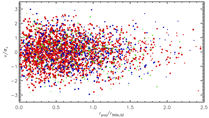
We create ensemble velocity distributions and phase-spaces by normalizing the peculiar velocity, $v_{p}$ , of each cluster member galaxy by the estimated velocity dispersion of its host cluster and the projected radial separation, $r_{\mathrm{proj}}$ , between each galaxy and SZ-derived centroid of its host cluster, normalized by $r_{500c,\mathrm{SZ}}$ for its host cluster. We compute $r_{500c,\mathrm{SZ}}$ for each cluster as the radius within which the mean density is equal to 500 times the critical density at the cluster redshift, based on the SZ mass estimate for each cluster (Hasselfield et al., 2013; Bleem et al., 2015). This produces normalized $v_{p}$ and $r_{\mathrm{proj}}$ values for each galaxy that are derived from independent observations: velocity dispersions and the SZ, respectively. Our cluster sample is comprised entirely of SZ-selected systems that are among the most massive clusters in the Universe (M ${}_{500c}\gtrsim 3\times 10^{14}$ $M_{\sun}$ h ${}_{70}^{-1}$ ; Bleem et al., 2015). This commonality in selection and mass supports the assumption that the ensemble phase-spaces that we construct are reliable representations of the average properties of the clusters used to populate them. The full-sample ensemble phase-space for our cluster sample is shown in Figure 2.

3.2 Velocity Segregation By Spectral Type

Table 4: Ensemble Dispersions By Galaxy Sub-population

Galaxy Subset	N_gals	$\sigma_{v}/\sigma_{\mathrm{v,all}}$	AD Prob^a^aA value of 0.1 indicates a 10% probability that galaxies in a given sub-population have a peculiar velocity distribution that is consistent with being Gaussian.
Passive	2028	$0.947\pm 0.015$	0.385
Post-starburst	274	$1.034\pm 0.044$	0.25
Star-forming	539	$1.110\pm 0.031$	0.388
Bright ( $m<m^{*}-0.5$ )	298	$0.894\pm 0.041$	$<1$ e $-9$ ^b^bThe approximation that we use from Hou et al. (2009) becomes imprecise at very large values of statistical significance.
Faint ( $m>m^{*}+0.5$ )	1107	$1.01\pm 0.021$	0.33

Note. — Here we show the results of statistical tests of different sub-populations of galaxies in the ensemble stack. From left to right the columns are: (1) the sub-population of galaxies analyzed, (2) the total number of galaxies of that sub-population that are in the ensemble, (3) the velocity dispersion of the galaxies in that sub-population, normalized to the velocity dispersion of the full ensemble, and (4) the probability that galaxies in that sub-population are drawn from a Gaussian velocity distribution based on the Anderson-Darling (AD) statistic.

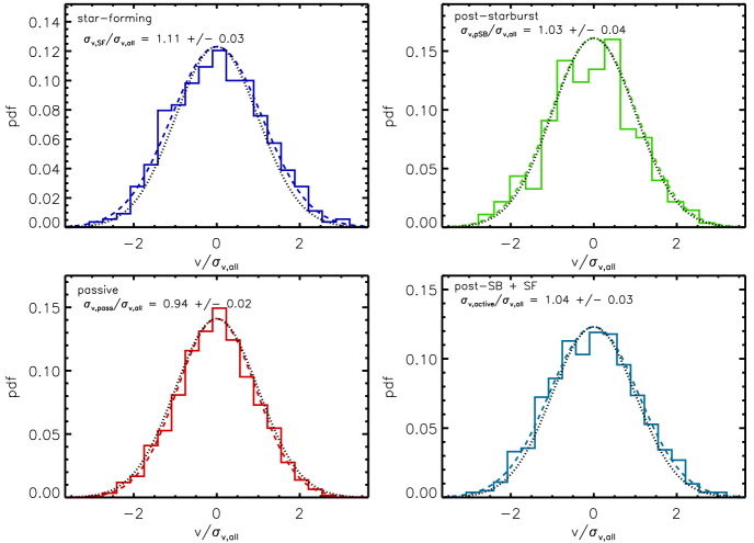
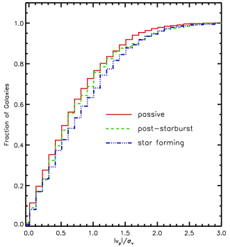
The ensemble cluster contains 2847 galaxies, 2841 of which have spectral classifications. We analyze the ensemble of 2841 galaxies with known spectral types, and generate the velocity distributions for passive, post-starburst, and star-forming cluster members, shown in Figure 3. We also plot the cumulative distribution functions (CDFs) of the absolute peculiar velocities of the same three types of cluster member galaxies (Figure 4). Qualitatively there is a clear trend in both Figures 3 & 4, with the star-forming galaxies having a larger velocity dispersion than the full ensemble, and tending to have larger absolute peculiar velocities than post-starburst and passive galaxies. Passive galaxies, on the other hand, have a smaller velocity dispersion relative to the full ensemble and tend to have smaller absolute peculiar velocities. Post-starburst galaxies represent the evolutionary “in-between” step between star-forming and passive galaxies and, interestingly, they also tend to lie in between passive and star-forming galaxies in velocity space for massive galaxy clusters.

Quantitatively we measure the magnitude of velocity segregation by galaxy type by performing a resampling of the ensemble distribution. Specifically, we generate 1000 Monte Carlo realizations of velocity distributions using only galaxies of the same type, where each realization is constructed by drawing 125 galaxies without replacement from the ensemble cluster, where “without replacement” here simply means disallowing any galaxy in the ensemble dataset from appearing more than once in a resampled realization. It is important to draw without replacement when performing a resampling analysis in which the 2nd order statistic (i.e., the dispersion) is being investigated, because allowing replacement draws will artificially bias the recovered dispersions low. The choice to use 125 galaxies is made to ensure good statistical precision in the dispersion estimate from each resampled dataset, while also allowing us to generate sufficient unique realizations from our ensemble so as to recover a good estimate of the spread in dispersion values—i.e., the statistical uncertainty in the velocity dispersion for each sub-population of galaxies.

We find that passive cluster members have a normalized velocity dispersion of $0.947$ $\pm$ $0.015$ relative to the entire cluster sample, while the corresponding velocity dispersion for star-forming galaxies is $1.110$ $\pm$ $0.031$ . Post-starburst galaxies actually have a velocity distribution that is indistinguishable from the total member galaxy distribution ( $\sigma_{v,PSB}/\sigma_{all}=1.034$ $\pm$ $0.044$ ), which is likely the result of a combination of two factors: 1) the post-starburst measurement is noisier because post-starbursts are $<10\%$ of our sample, and 2) post-starburst galaxies are a transitional population between the star-forming and passive populations. The differences between the passive and star-forming galaxy velocity dispersion is significantly larger than the statistical uncertainties ( $>3\sigma$ ). Directly comparing the velocity dispersion of passive and star-forming galaxies we find the star-forming galaxies have a dispersion $17$ $\pm$ $4$ % larger than the passive cluster galaxy population.

One other factor to consider is the target prioritization strategy we used when designing the multi-slit masks that produced our spectra. As described in Ruel et al. (2014) and Bayliss et al. (2016), we selected targets based on photometric colors. Red-sequence selected candidate member galaxies were given top priority, with potential blue-cloud galaxies making up the next priority level, and all other sources used as filler objects. In principle this strategy could bias our radial sampling to preferentially yield spectra of passive (i.e., red-sequence) galaxies at smaller projected cluster-centric radii. However, in practice we find that the projected radial distribution of slits with different priorities is relatively flat. We also note that the average peculiar velocities of all cluster member galaxies, regardless of type, tend to decrease with increasing projected radius, so that the impact of a prioritization bias that skewed our non-passive galaxy samples to larger projected radii would only serve to slightly suppress any velocity segregation signal.

It is also important here to consider the possible impact of interloper galaxies that we have mistakenly included as members in our galaxy spectroscopy sample. We cannot realistically expect to identify member galaxies with perfect accuracy, and so interlopers are almost certainly present at some level. That being said, we also point out that analysis of the effects of interlopers in simulations suggests that they do not strongly bias velocity dispersion estimates with radial sampling similar to ours. Saro et al. (2013) studied the effects of red sequence (i.e., passive galaxy) interlopers in simulations, finding that interloper fractions remain small ( $\lesssim$ 7%) within projected radii $r_{\mathrm{proj}}\lesssim r_{200c}$ (where $r_{200c}$ is the radius within which the mean density is 200 times the critical density); this suggests that we can expect our cluster data to typically include of order 1-2 interlopers per cluster. Saro et al. (2013) found that these small numbers of red-sequence interlopers, when included, act to boost the estimated velocity dispersions of clusters. Biviano et al. (2006) explored the effects of blue/star-forming galaxies, which are much more common in the field, as an interloper population and found that they actually have the effect of suppressing the estimated velocity dispersions of clusters. These simulation results indicate that the effects of passive and star-forming interloper galaxies may both act to suppress an underlying velocity segregation signal by galaxy type.

Statistical tests are also helpful to quantify the significance of our detection of velocity segregation by galaxy type, and here we employ both the Kolmogorov-Smirnov (KS) and the Anderson-Darling (AD) tests. The KS test is a tool that is commonly used to quantitatively compare distributions. It is useful for identifying differences near the centers of probability distributions, but lacks power in the wings. The AD test, on the other hand, is sensitive to deviations from the centers out through the wings of distributions, and has been demonstrated to be a much more powerful test for detecting differences between CDFs than the KS test (e.g., Hou et al., 2009). Both the KS and AD test results are consistent with each of the passive, post-starburst, and star-forming galaxy populations having Gaussian velocity distributions. Of these the post-starburst galaxies have the largest probability of rejecting the null hypothesis at 25% ( $\sim 1.2\sigma$ ). The normalized velocity dispersions for passive/post-starburst/star-forming galaxies are given in Table 4, along with the AD test probabilities that each galaxy type’s velocity distribution is Gaussian.

When we compare the distributions of different galaxy types against one another we find that the KS test identifies a $\sim$ 1.6 $\sigma$ difference between the passive and star-forming galaxy distributions, while the comparison with the AD test produces a $\gtrsim 6\sigma$ difference, but neither the KS nor AD tests identify statistically significant differences between the other pairings of galaxy subsets. We point out here that the formula that we use to convert AD statistic values into confidence levels for rejecting the null hypothesis (Hou et al., 2009) is a numerical approximation that becomes imprecise once the statistical significance becomes very large, but is more than adequate for our purposes where we are primarily interested in testing whether we can confidently reject the null hypothesis.

We also use the AD test to quantify deviations from Gaussianity in the ensemble velocity distributions of passive, post-starburst, and star-forming galaxies, and find that all three spectral types are consistent with Gaussian velocity distributions.

3.2.1 Trends With Projected Cluster Radius

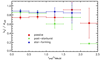
Having detected segregation effects between velocity distributions of galaxies differentiated by spectral type, we now expand our analysis to test for possible trends as a function of other quantities. The average peculiar velocities of passive, post-starburst, and star-forming galaxies are plotted in radial bins of width $0.5r_{500c,\mathrm{SZ}}$ in Figure 5. From Figure 5 we see that the passive galaxies have consistently smaller dispersions than the star-forming galaxies in the more central radial bins where our spectroscopic data is more numerous and the uncertainties smallest ( $r_{\mathrm{proj}}\leq 1.5r_{500c,\mathrm{SZ}}$ ). The outer radial bins are less well sampled, with larger uncertainties, and so it is difficult to draw firm conclusions from the data, and are also where the sample should be more likely to suffer from some contamination by interloping galaxies because the cluster over-density is smallest at larger radii. While we see no strong trends in radius for any sub-population of galaxies, we do note a low-significance drop in the peculiar velocities of star-forming galaxies at larger radii, while passive galaxy peculiar velocities are flat with radius, within the uncertainties. This trend would be consistent with studies that find star-forming galaxies to preferentially have radially-elongated orbits, while passive galaxy orbits have larger tangential components (Katgert et al., 1996; Biviano & Katgert, 2004), and makes sense in the context of a physical picture in which star-forming cluster member galaxies reflect a population of galaxies that have recently fallen into the cluster potential while passive galaxies tend to have been in the cluster for longer times and are more dynamically relaxed (Mahajan et al., 2011; Haines et al., 2015).

3.2.2 Trends With Cluster Redshift

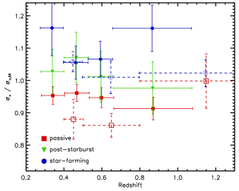
Our galaxy cluster sample has the benefit of an approximately flat selection in mass, despite spanning a relatively wide range in redshift. We can, therefore, divide the sample up into redshift bins to investigate possible trends in the velocity segregation effects in clusters of similar masses as a function of redshift. We define four redshift bins that are chosen to place a similar number of cluster member galaxies in each bin; the redshift intervals we use and the velocity dispersion of galaxies of each spectral type are given in Table 5. Each bin contains at least 83 galaxies of each spectral type, ensuring good statistical significance on the estimated dispersion of each sub-population in each redshift bin.

The data are shown in Figure 6, and it is clear that the tendency for star-forming galaxies to have larger velocity distributions than passive galaxies holds out to $z\gtrsim 1$ in our data, though the individual estimates become noisier due to poorer statistical sampling as a result of dividing the sample. For comparison we also show the recently published results from Barsanti et al. (2016) as open symbols with dashed error bars, which are generally in good agreement with our measurements, especially at $z\lesssim 0.8$ . The offsets between our data and the Barsanti et al. (2016) measurements are likely a result of slightly different compositions of our respective datasets with respect to the fraction of the data for passive vs. star-forming member galaxies. That is to say, both analyses use all available member galaxies to compute $\sigma_{\mathrm{v,all}}$ for each cluster, which normalizes the peculiar velocities in the ensemble, and if the number of passive vs. star-forming galaxies that are used is different between our two datasets then the fiducial $\sigma_{\mathrm{v,all}}$ velocity dispersion will change. A sample with more blue/star-forming galaxies would have, on average, a systematically larger $\sigma_{\mathrm{v,all}}$ estimated for each cluster, while a more red/passive galaxy heavy dataset would have smaller values of $\sigma_{\mathrm{v,all}}$ . Larger values of $\sigma_{\mathrm{v,all}}$ would obviously result in smaller values of the ratios of the dispersions of both passive and star-forming subsets, relative to $\sigma_{\mathrm{v,all}}$ , while the opposite is true for smaller values of $\sigma_{\mathrm{v,all}}$ . Notably, the Barsanti et al. (2016) sample tends to include relatively more blue/star-forming member galaxies than ours, and accordingly their measurements of the red/blue galaxy dispersions normalized to $\sigma_{\mathrm{v,all}}$ are shifted systematically low relative to ours. Ideally we might prefer to use the dispersions measured using only passive galaxies as the normalizing dispersion for each individual cluster. However, doing so with our current dataset would result in much higher statistical uncertainty in the normalizing dispersion used for each cluster, and severely degrade our ability to detect the signatures of velocity segregation.

Table 5: Ensemble Galaxy Clusters Grouped By Redshift

Redshift Interval	N_gals	N_PASS	N_PSB	N_SF	$\sigma_{v,PASS}/\sigma_{\mathrm{v,all}}$	$\sigma_{v,PSB}/\sigma_{\mathrm{v,all}}$	$\sigma_{v,SF}/\sigma_{\mathrm{v,all}}$
$z\leq 0.4$	757	599	85	93	$0.953\pm 0.028$	$1.027\pm 0.069$	$1.162\pm 0.086$
$0.4<z\leq 0.53$	842	604	87	168	$0.961\pm 0.026$	$1.071\pm 0.078$	$1.055\pm 0.052$
$0.53<z\leq 0.66$	718	483	86	165	$0.947\pm 0.031$	$1.012\pm 0.079$	$1.066\pm 0.056$
$z>0.66$	527	343	83	114	$0.913\pm 0.035$	$0.976\pm 0.082$	$1.161\pm 0.072$

Note. — Here we show the results of dividing our ensemble cluster into four redshift bins. The columns are: (1) the redshift intervals four each bin, (2) the total number of cluster member galaxies in each bin, (3) the total number of passive member galaxies in each bin, (4) the total number of post-starburst member galaxies in each bin, (5) the total number of star-forming member galaxies in each bin, (6) the velocity dispersion of passive galaxies in each bin relative to the full ensemble, (7) the velocity dispersion of post-starbust galaxies in each bin relative to the full ensemble, (8) velocity dispersion of star-forming galaxies in each bin relative to the full ensemble.

The Barsanti et al. (2016) analysis is essentially identical to our own except that galaxies are split into two “red” and “blue” sub-populations based on color for the large majority of their data. These red and blue groups should translate approximately to isolating passive and actively star-forming galaxies, where the galaxies that we classify as post-starburst could be flagged as either passive (“red”) or star-forming (“blue”) galaxies, depending on the exact galaxy and color cut. The Barsanti et al. (2016) cluster sample is drawn from the literature and spans a wide range in redshift, so the red/blue color cut varies by cluster and the available photometry. This should have the effect of introducing some effective noise into the process of classifying galaxies in color space, so that there is almost certainly not a perfect mapping between “red” galaxies and those which would be spectroscopically classified as passive, nor between “blue” and those which would be spectroscopically classified as star-forming. These classification differences can easily explain slight differences between velocity segregation measurements between our work and the Barsanti et al. (2016) results, though there is good quantitative agreement, within the uncertainties, between our two results at lower redshift, which suggests that any effects due to differences in classifying galaxy types are likely sub-dominant relative to the statistical uncertainties.

There is some evidence in the Barsanti et al. (2016) data for an easing of the velocity segregation between blue and red galaxies in their very broad high-z bin ( $0.8<z<1.5$ ). Our measurements indicate that velocity segregation in our clusters between passive and star-forming galaxies is very strong in a bin spanning $0.66<z<1.08$ , which could suggest that if the velocity segregation by galaxy color/spectral type occurs, it must be happening in clusters above $z\gtrsim 1.1$ . Our results are also consistent with another recent study by Biviano et al. (2016) of ten clusters in the redshift interval $0.87\lesssim z\lesssim 1.2$ from the Gemini Cluster Astrophysics Spectroscopic Survey (GCLASS; Muzzin et al., 2012) in which the ratio of velocity dispersions of passive to star-forming galaxies is measured to be $\simeq 0.88$ .

3.3 Velocity Segregation By Relative Luminosity

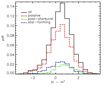
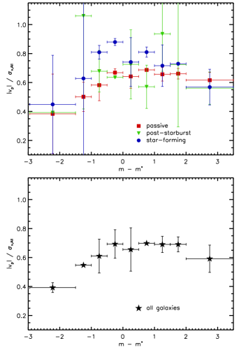
With photometry in hand for the majority of our galaxy spectroscopy sample we can also investigate velocity segregation effects as a function of galaxy luminosity. We use cluster galaxy brightness measurements in units relative to $m^{*}$ , a standard quantity that can be easily incorporated into both observational data and simulated clusters (Cole et al., 2001; Cohen, 2002; Rudnick et al., 2006, 2009). Specifically, we use $m^{*}$ values computed from Bruzual & Charlot (2003) models in the same fashion as described in previous SPT publications (High et al., 2010; Song et al., 2012; Bleem et al., 2015). Figure 7 shows the distribution of cluster member galaxies with brightness measurements as described in § 2.4 plotted relative to the characteristic magnitude, $m^{*}$ , for the full cluster member sample as well as the subsamples of cluster members of different spectral types. We use these data, in combination with the normalized peculiar velocities of each cluster member in the ensemble to plot the expectation value for the absolute peculiar velocity of cluster members as a function of brightness for all galaxies together, as well as for each of the passive, post-starburst, and star-forming galaxy subsets (Figure 8). It is clear that the brightest galaxies—independent of spectral type—universally prefer smaller absolute peculiar velocities, and that when we treat all galaxies together we see a strong drop in the absolute peculiar velocities of galaxies brighter than $\sim m^{*}-0.5$ , while galaxies fainter than this tend to remain approximately flat in absolute peculiar velocity as a function of brightness. There is no statistically significant evidence in our data for an evolution in the presence or of velocity luminosity segregation with redshift. Specifically, if we split our sample into two redshift bins at $z=0.45$ —which optimally balances the number of bright galaxies in the high and low bins—we see the strong drop in peculiar velocity for bright galaxies in each of the high and low redshift bins.

This same qualitative effect has been observed in low redshift clusters (Chincarini & Rood, 1977; Biviano et al., 1992; Mohr et al., 1996; Goto, 2005; Old et al., 2013; Ribeiro et al., 2013). Barsanti et al. (2016) also recently observed a similar effect in an analysis of galaxy clusters drawn from the literature. Barsanti et al. (2016) follow work on low-z clusters by Biviano et al. (1992) and parameterize galaxy brightnesses relative to the third brightest cluster member in each cluster. We find this parameterization unreliable in our own data, where we can only make probabilistic statements about galaxy membership beyond the galaxies for which we have spectra. Instead we choose to parameterize brightness relative to an observable quantity that is universally available based on standard measurements of the galaxy luminosity function.

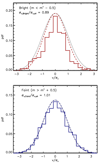
Motivated by the drop in peculiar velocity that we observe in Figure 8, we examine the properties of two luminosity-based sub-populations of cluster members: those brighter than $m^{*}-0.5$ (“bright”) and those fainter than $m^{*}+0.5$ (“faint”). The choice of the faint galaxy sample definition is somewhat arbitrary, but we find that the result is insensitive to the exact cut we use here, which is unsurprising in light of the behavior apparent in Figure 8. We also apply the AD statistic in the same manner as before (see § 3.2) to test whether each of these sub-populations of member galaxies have velocity distributions that are consistent with Gaussian. Once again we point out that the formula that we use to convert AD statistic values into confidence levels for rejecting the null hypothesis breaks down at very large values of statistical significance, but it is clear that the bright and faint galaxy samples are inconsistent with being drawn from the same underlying velocity distribution, and that the velocity distribution of bright galaxies is inconsistent with a Gaussian distribution at high significance ( $>6\sigma$ ; Table 4).

Moreover, when we plot the velocity distributions of these two galaxy subsets (Figure 9) we see that the bright galaxy population has a distinctly “peaky” shape with an excess of galaxies concentrated around small peculiar velocity values and a dearth of galaxies filling out what would be the middle wings of a Gaussian velocity distribution. This further helps to demonstrate the divergent kinematics of the brightest galaxies in clusters. The behavior that we see in the peculiar velocities of bright cluster galaxies would appear to be direct evidence of dynamical friction effects, which should be proportional to the mass of a galaxy, with larger dynamical friction effects acting on brighter/more massive galaxies.

4 Velocity Segregation and Biases in Velocity Dispersion Estimates

Velocity segregation measurements are a valuable probe of cluster assembly and the link between environment and galaxy evolution, but they also have tremendous potential as a link between observations and simulations of galaxy cluster velocity dispersions as a cosmological observable. In this section we quantify the biases in velocity dispersion estimates by incrementally varying the types of galaxies that are sampled from the ensemble cluster data, and we attempt to compare our measured biases to those of simulated galaxy clusters.

Specifically, we investigate the bias in the estimated velocity dispersion as a function of the fractions of passive/star-forming and bright/faint galaxies used. In all cases the bias that we measure is the bias relative to the full ensemble cluster dataset, and not the bias relative to the true velocity dispersion of dark matter particles in our galaxy cluster sample, which is, of course, unknown. We can then compare the biases that we measure to the same effects in simulated galaxy clusters where the true dark matter particle velocity dispersions are known. We advocate for the idea that comparing velocity dispersion biases associated with velocity segregation effects can serve as a bridge between observations and simulations (e.g.; Lau et al., 2010; Gifford et al., 2013; Saro et al., 2013) of galaxy cluster velocity dispersion measurements, potentially facilitating a kind of cross-calibration of velocity dispersions in observations and simulations.

4.1 Velocity Dispersion vs. Fraction of Red/Blue Galaxies Used

We first estimate velocity dispersions for resampled subsets of our ensemble galaxy cluster data while varying the fraction of passive and star-forming galaxies included in each resampled cluster realization. We essentially repeat the Monte Carlo resampling described above in § 3.2, in which each realization is made up of 125 galaxies drawn without replacement from the ensemble cluster, but now generate realizations in which we vary the fraction of the resampled cluster that is composed of a specific galaxy type. This exercise is performed with an eye toward comparing our results to those from simulations in the literature (e.g., Gifford et al., 2013). In simulation-based work galaxies are often separated by color rather than precise spectral type. This means that there is some ambiguity about how to treat the post-starburst galaxies in our sample when comparing to other binary red vs. blue analyses, as we have already touched on above in § 3.2.2. In light of this ambiguity we generate resampled datasets while varying the fraction of both the passive and star-forming fractions by regular intervals. When we generate resampled realizations in which we control the passive fraction we are randomly filling the remaining (non-passive) fraction using all of the non-passive galaxies (i.e., all post-starburst and star-forming galaxies). When we control the fraction of star-forming galaxies, on the other hand, then we use both post-starburst and passive galaxies to fill the remaining non-star-forming fraction of each realization.

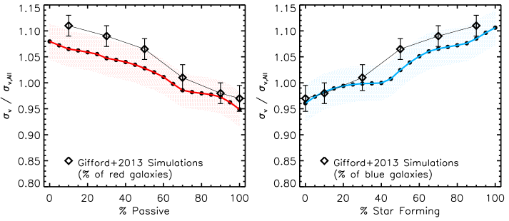
The results of this resampling procedure are shown in Figure 10 along with simulation results from Gifford et al. (2013) for comparison. Qualitatively, there is good agreement between our data and simulations regarding the shape of the trend with red/blue fraction, independent of how post-starburst galaxies are treated. There is, however, a systematic offset between the normalized velocity dispersions measured in simulations and in our data. This offset is marginally larger when we group post-starburst galaxies in with star-forming galaxies, perhaps suggesting that the color cuts applied by Gifford et al. (2013) preferentially sort the simulated analogs of post-starburst galaxies in with the passive galaxies. In the case where we treat passive and post-starburst galaxies together as non-star-forming, we see the closest agreement between our measurements and the simulations with our data lying consistently low relative to the simulations.

The exact interpretation of the offset is complicated, however, by the fact that the reference velocity dispersion ( $\sigma_{\mathrm{v,all}}$ ) is different in our data compared to the simulations. We use the velocity dispersion of our full ensemble dataset as the reference value, but clusters in simulations are plotted relative to the true underlying dark matter particle velocity dispersions, $\sigma_{\mathrm{DM}}$ , a quantity that scales well with cluster virial masses in simulations (Evrard et al., 2008). We discuss this offset in more detail in § 5.1 below.

4.2 Velocity Dispersion vs. Fraction of Bright/Faint Galaxies Used

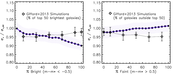
There is a significant caveat associated with making direct comparisons between our measurements and the simulation results from Gifford et al. (2013). Specifically, we do not have the same perfect knowledge of cluster membership that is available for a simulated cluster sample, and so we cannot generate a true ranking of the N brightest galaxies. Also, it is unlikely that we would rarely, if ever, be able to obtain spectra for each of the brightest 50 member galaxies per cluster—as Gifford et al. (2013) do in simulations—for a real sample of clusters. It is certainly a useful exercise, however, to compare the relative offset in the velocity dispersion that we measure as we vary the fraction of bright vs. faint galaxies against predictions for a similar resampling in simulations. Our measurements, along with simulation results from varying the fraction of the 50 brightest members used, are shown in Figure 11. Here, again, we see the effects of the velocity segregation by galaxy luminosity, where we measure smaller dispersions for realizations comprised mostly or entirely of bright galaxies. Specifically, the velocity dispersions consistently fall as the fraction of bright galaxies increases, reaching a $\sim 10$ % bias (low) for a pure bright galaxy dispersion (see § 3.3). The simulations, however, do not exhibit the same effect, with dispersions biased only $\sim 2\pm 2$ % low when using the 50 brightest galaxies to measure the dispersion.

Similar to the above, we also measure the velocity dispersion in resampled datasets where we vary the fraction of faint galaxies used, and compare this to the reverse of the simulation result. Here we see a weak trend with the fraction of faint galaxies used, finding velocity dispersions that are biased low by $\sim 3\pm 3$ % when using no faint galaxies, and high by $\sim 1\pm 3$ % low for a sample composed entirely of faint galaxies. We can interpret the slightly stronger bias for a sample using no faint galaxies as a manifestation of the velocity segregation of the brightest galaxies discussed in § 3.3. There the “0% faint galaxies” realizations include only galaxies brighter than $m^{*}+0.5$ , which will naturally include a substantial fraction of the bright galaxy sample ( $m<m^{*}-0.5$ ).

5 Discussion and Implications

There is a general consensus in the literature about the underlying astrophysical causes of velocity segregation effects by galaxy color or spectral/morphological type. Differences between passive/star-forming galaxies are understood to be related to the fact that actively star-forming galaxies in clusters are predominantly galaxies that are either in the process of falling into the cluster, or have recently done so (Moss & Dickens, 1977; Carlberg et al., 1997a; Goto, 2005). Biviano & Katgert (2004) have made a more sophisticated argument, claiming that star-forming cluster galaxies tend to be in approximate equilibrium with their cluster potentials but have orbital trajectories that are preferentially radial, while passive cluster galaxies have orbits that more closely resemble the random motions that would normally be associated with virialized test particles in a gravitational potential.

Differences in the shapes of the orbital paths of star-forming vs. passive galaxies would be a natural consequence of the argument that star-forming galaxies are more recently accreted, and their preferentially radial orbits reflect the fact that they have not yet experienced sufficient dynamical interactions within the cluster to acquire the more random orbits. These are all essentially differently-phrased arguments that star-forming member galaxies are, on average, less (or not yet) virialized, while passive member galaxies are virialized; these arguments are consistent with low-z studies and analyses of simulations aimed at understanding cluster assembling and in-fall (Mahajan et al., 2011; Haines et al., 2015).

Similarly, there is general agreement about the astrophysical effects responsible for velocity segregation between more and less luminous galaxies. This effect can be explained by physical processes such as dynamical friction (also called dynamical breaking) that cause transfers of kinetic energy from larger galaxies to smaller galaxies, as well as gravitational interactions that can convert bulk kinetic energy into internal kinetic energy via, for example, accelerating and ejecting individual stars during galaxy mergers (Sarazin, 1986; Kashlinsky, 1987; Biviano et al., 1992; Mahajan et al., 2011). It is mildly puzzling that the velocity segregation effect that we see in our data for the brightest and faintest galaxies does not appear in some recent simulations; we are not the first to detect this signal in bright cluster member galaxies, (Chincarini & Rood, 1977; Biviano et al., 1992; Mohr et al., 1996; Goto, 2005; Ribeiro et al., 2010; Old et al., 2013; Barsanti et al., 2016), and the effect is seen in some simulations (e.g., Lau et al., 2010; Saro et al., 2013). We are wary of over-interpreting this discrepancy, because of the difference in our bright galaxy sample and the 50 brightest members approach used by Gifford et al. (2013), but it is possible that the discrepancy is related to the effects of missing baryonic/gas physics that are not captured in dark matter only simulations. We elect not to speculate too much about the pros and cons of various methods for the treatment of halos in simulated clusters, and how mock galaxies are placed into those halos, though it is not unreasonable to suppose that different prescriptions could generate significantly different results. Certainly the measurement we present here could represent useful benchmark test to be reproduced in future simulations. Looking forward we believe it is important that both observers and simulators strive to find useful quantities that can be measured in both data and simulations; it is with this in mind that we analyze galaxies in our sample in terms of relative luminosity, scaled by the characteristic magnitude, $m^{*}$ .

5.1 Velocity Segregation As A Tool To Calibrate Velocity Dispersion Estimates

One of our primary objectives in this work is to test for the presence of systematic biases in velocity dispersion estimates, and to attempt to connect our results to simulations that explore the same or similar effects. In § 4 we show the biases in velocity dispersions that are estimated using cluster data realizations in which we control the fractions of passive and star-forming galaxies. Figure 10 demonstrates that we see the same general behavior as simulations in the change in velocity dispersion biases as a function of the fraction of passive and star-forming galaxies used to estimate the velocity dispersion. However, there is a small offset in the normalization of those biases between our data and the simulations. Independent of how we treat post-starburst galaxies in our analysis, whether they are grouped in with passive or star-forming galaxies, the velocity dispersions estimated from data as a function of galaxy type are offset low by as much as $\sim 3$ % relative to the simulations. This offset is more pronounced for realizations comprised mostly or entirely of star-forming galaxies (and for those using few or no passive galaxies), reaching peak values of $\gtrsim 3$ % when the fraction of star-forming galaxies exceeds 50% (or when the fraction of passive galaxies is less than 50%).

Here we explore the idea that these offsets may have implications for calibrating cluster velocity dispersion measurements relative to simulations. First, we consider the contribution of interlopers to the biases that we see, as it is likely that interloping star-forming galaxies in our ensemble datasets are contributing to some degree to the observed offset. As we have already mentioned, studies show that the inclusion of interloping star-forming field galaxies has the effect of driving velocity dispersion estimates to smaller values (Biviano et al., 2006). Saro et al. (2013) have also shown that velocity dispersions estimated using passive galaxies with large interloper fractions are biased high. We see no evidence of our dispersions being biased high relative to simulations, suggesting that passive galaxy interlopers are not strongly affecting our observations.

Interloper effects are one of several different factors that can systematically bias galaxy velocity dispersions measurements. One interpretation that we can consider regarding the small offset that we observe in Figure 10 is that we are effectively measuring a form of velocity bias, $b_{\mathrm{v}}$ , between our galaxy velocity dispersion measurements and true underlying dark matter dispersions of our galaxy clusters. The standard definition of the velocity bias is $b_{\mathrm{v}}=\sigma_{\mathrm{gal}}/\sigma_{\mathrm{DM}}$ , i.e., the normalization between the true dark matter velocity dispersion and the velocity dispersion of cluster member galaxies. Efforts have been made in the past to quantify velocity bias in several different ways, with a wide range of results ( $b_{\mathrm{v}}\simeq 0.95-1.3$ ; Colín et al., 2000; Ghigna et al., 2000; Diemand et al., 2004; Faltenbacher & Diemand, 2006; Lau et al., 2010; White et al., 2010; Saro et al., 2013; Wu et al., 2013), but to our knowledge this is the first attempt to recover an estimate of velocity bias at $z>0.1$ by comparing velocity segregation effects from data and simulations. In this context our comparison suggests that velocity segregation measurements may provide a direct way to compare systematic biases in velocity dispersion as measured in real clusters and in simulations, providing a means of cross-calibrating velocity dispersion data and cosmological simulations.

When discussing velocity bias it is important to distinguish between velocity bias measurements in simulations, where both the true dark matter particle velocity dispersion and true cluster membership properties of galaxies are known, and in data like ours, where we do not know either. The offset that we detect in our data could be interpreted as a detection of what we might call the effective velocity bias, which we define as:

b_{\mathrm{v,obs}}=\frac{\sigma_{\mathrm{gal,obs}}}{\sigma_{\mathrm{DM}}}=\frac{\sigma_{\mathrm{gal,obs}}}{\sigma_{\mathrm{gal,sims}}}\times\frac{\sigma_{\mathrm{gal,sims}}}{\sigma_{\mathrm{DM}}}

(1)

This is a quantity that is specific to our data and the Gifford et al. (2013) simulations, in that it describes the offset that we observe between the velocity segregation trend between the two. A variety of different biases/effects can be folded into this effective velocity bias term, including dynamical friction (which should, in principle, suppress the peculiar velocities of all member galaxies at some level), the effects of sub-halos within the larger cluster halo potentials, and measurement effects such as interlopers. However, as a practical matter it is not necessarily important that we are able to suss out the individual factors that determine the effective velocity bias for our cluster spectroscopy, because $b_{\mathrm{v,obs}}$ is the quantity of interest if one aims to use velocity dispersions as accurate proxies for total cluster masses. We find that our measurements are offset $\sim 0-3$ % low, which implies a value for $b_{\mathrm{v,obs}}\simeq 0.97-1.0$ , where the bias varies with different fractions of passive vs. star-forming galaxies used to measure the velocity dispersion. In principle, these numbers could be used to calibrate our measured dispersions to be in agreement with simulations—in this case specifically with the simulations analyzed by Gifford et al. (2013).

There are several important caveats to bear in mind regarding this effective velocity bias. Firstly, there is potentially a systematic uncertainty in our velocity segregation measurements that results from the varying fraction of passive vs. star-forming galaxies in our individual galaxy data (Table 2). This effect would manifest as a difference—certainly a scatter and potentially a bias—between the first ratio on the far right side of Equation 1 as applied to the full ensemble and the individual clusters that were used to generate that ensemble. The ideal dataset would avoid this systematic effect by having a constant ratio of passive to star-forming galaxies across all clusters, a feat that would be difficult to achieve in practice.

Secondly, different simulations measure different biases between the dispersions of dark matter and mock galaxies, so we might expect to recover a different offset between our data and different simulations. These differences would manifest as differences in the second ratio on the far right side of Equation 1. This represents an underlying systematic uncertainty that emerges from fundamental differences between simulations—e.g., volume, resolution, dark matter only vs. hydrodynamical— as well as from how those simulations are populated with galaxies. We cannot address that systematic uncertainty based on our comparison to the Gifford et al. (2013) simulations alone. That said, this is an exciting step toward quantifying this systematic uncertainty, which is essential to using velocity segregation to precisely calibrate dispersion measurements.

6 Summary & Conclusions

We have analyzed spectroscopy of 4148 galaxies (2868 cluster members) in the fields of 89 massive, SZ-selected galaxy clusters. We detect signatures of velocity segregation as a function of both galaxy type and relative luminosity at high significance. We measure the velocity dispersion of star-forming galaxies in our cluster ensemble to be $17\pm 4$ % larger than the passive galaxy population, and that this velocity segregation holds for our entire cluster sample, which extends to $z\sim 1.1$ . There is a strong drop-off in the average absolute peculiar velocity of cluster member galaxies brighter than $m^{*}-0.5$ , with galaxies satisfying that criterion having a velocity dispersion $11\pm 4$ % smaller than the velocity dispersion of the full cluster member ensemble. For the brightest galaxies we find a highly distorted velocity distribution that is statistically confirmed to differ from a Gaussian distribution at high significance. Finally, we compare our velocity segregation measurements to similar measurements in recent simulations, and see a qualitative agreement for passive vs. star-forming cluster member galaxies, albeit with what appears to be a systematic bias between the data and simulations. We consider the implications of interpreting this systematic bias as a detection of the effective velocity bias that describes the scaling between the observed velocity distribution of galaxies in clusters and the intrinsic velocity dispersion of dark matter particles in clusters, $b_{\mathrm{v,obs}}\simeq 0.97-1.0$ . Our result is encouraging for the prospect of using velocity segregation effects in galaxy cluster spectroscopy samples to calibrate velocity dispersion measurements against simulations.

Gemini-S (GMOS), Magellan:Baade (IMACS), Magellan:Clay (LDSS3), VLT:Antu (FORS2)

We thank Cristóbal Sifón for sharing reduced 1D spectra from his 2013 paper so that it could be included in our analysis. This work has been supported by NSF grant AST-1009012. Work at Argonne National Laboratory was supported under U.S. Department of Energy contract DE-AC02-06CH11357. DR is supported by a NASA Postdoctoral Program Senior Fellowship at the NASA Ames Research Center, administered by the Universities Space Research Association under contract with NASA. Data presented here include observations from the Gemini Observatory, which is operated by the Association of Universities for Research in Astronomy, Inc., under a cooperative agreement with the NSF on behalf of the Gemini partnership: The United States, Canada, Chile, Australia, Brazil, and Argentina. Gemini data used in this work was taken as a part of Gemini programs awarded to PI Mohr (GS-2009B-Q-16) and PI Stubbs (GS-2011A-C-03, GS-2011A-C-04, GS-2011B-C-06, GS-2011B-C-33, GS-2012A-Q-04, GS-2012A-Q-37, GS-2012B-Q-29, GS-2012B-Q-59, GS-2013A-Q-05, GS-2013A-Q-45, GS-2013B-Q-25, GS-2013B-Q-72, GS-2014B-Q-31, GS-2014B-Q-64). This paper also uses spectroscopic data gathered with the 6.5-meter Magellan Telescopes located at Las Campanas Observatory, Chile. Time was allocated through Harvard-CfA (PIs Bayliss, Brodwin, Foley, and Stubbs) and the Chilean National TAC (PI Clocchiatti). We also make use of spectroscopy from 8.1m Very Large Telescope (VLT) time granted through DDT (PI Carlstrom, 286.A-5021) and ESO (PI Bazin, 087.A-0843, and PI Chapman, 285.A-5034 and 088.A-0902).

References

Abraham et al. (1996) Abraham, R. G., Smecker-Hane, T. A., Hutchings, J. B., et al. 1996, ApJ, 471, 694
Allen et al. (2011) Allen, S. W., Evrard, A. E., & Mantz, A. B. 2011, ARA&A, 49, 409
Bahcall et al. (1991) Bahcall, J. H., Beichman, C. A., Canizares, C., et al. 1991, The Decade of Discovery in Astronomy and Astrophysics (Astronomy and Astrophysics Survey Committee, National Research Council, National Academy Press, Washington, D. C.)
Bahcall (1981) Bahcall, N. A. 1981, ApJ, 247, 787
Balogh et al. (1999) Balogh, M., Babul, A., & Patton, D. 1999, MNRAS, 307, 463
Balogh et al. (1997) Balogh, M. L., Morris, S. L., Yee, H. K. C., Carlberg, R. G., & Ellingson, E. 1997, ApJ, 488, L75
Balogh et al. (2000) Balogh, M. L., Navarro, J. F., & Morris, S. L. 2000, ApJ, 540, 113
Barsanti et al. (2016) Barsanti, S., Girardi, M., Biviano, A., et al. 2016, A&A, 595, A73
Bayliss et al. (2011) Bayliss, M. B., Hennawi, J. F., Gladders, M. D., et al. 2011, ApJS, 193, 8
Bayliss et al. (2014) Bayliss, M. B., Ashby, M. L. N., Ruel, J., et al. 2014, ApJ, 794, 12
Bayliss et al. (2016) Bayliss, M. B., Ruel, J., Stubbs, C. W., et al. 2016, ApJS, 227, 3
Beers et al. (1990) Beers, T. C., Flynn, K., & Gebhardt, K. 1990, AJ, 100, 32
Benson et al. (2013) Benson, B. A., de Haan, T., Dudley, J. P., et al. 2013, ApJ, 763, 147
Biviano et al. (1992) Biviano, A., Girardi, M., Giuricin, G., Mardirossian, F., & Mezzetti, M. 1992, ApJ, 396, 35
Biviano et al. (1993) —. 1993, ApJ, 411, L13
Biviano & Katgert (2004) Biviano, A., & Katgert, P. 2004, A&A, 424, 779
Biviano et al. (1997) Biviano, A., Katgert, P., Mazure, A., et al. 1997, A&A, 321, 84
Biviano et al. (2002) Biviano, A., Katgert, P., Thomas, T., & Adami, C. 2002, A&A, 387, 8
Biviano et al. (2006) Biviano, A., Murante, G., Borgani, S., et al. 2006, A&A, 456, 23
Biviano & Poggianti (2009) Biviano, A., & Poggianti, B. M. 2009, A&A, 501, 419
Biviano et al. (2016) Biviano, A., van der Burg, R. F. J., Muzzin, A., et al. 2016, A&A, 594, A51
Biviano et al. (2013) Biviano, A., Rosati, P., Balestra, I., et al. 2013, A&A, 558, A1
Bleem et al. (2015) Bleem, L. E., Stalder, B., de Haan, T., et al. 2015, ApJS, 216, 27
Bocquet et al. (2015) Bocquet, S., Saro, A., Mohr, J. J., et al. 2015, ApJ, 799, 214
Borgani et al. (1997) Borgani, S., da Costa, L. N., Freudling, W., et al. 1997, ApJ, 482, L121
Bothun (1982) Bothun, G. D. 1982, ApJS, 50, 39
Brodwin et al. (2010) Brodwin, M., Ruel, J., Ade, P. A. R., et al. 2010, ApJ, 721, 90
Brodwin et al. (2013) Brodwin, M., Stanford, S. A., Gonzalez, A. H., et al. 2013, ApJ, 779, 138
Bruzual & Charlot (2003) Bruzual, G., & Charlot, S. 2003, MNRAS, 344, 1000
Carlberg et al. (1997a) Carlberg, R. G., Yee, H. K. C., Ellingson, E., et al. 1997a, ApJ, 485, L13+
Carlberg et al. (1997b) —. 1997b, ApJ, 476, L7
Carlstrom et al. (2011) Carlstrom, J. E., Ade, P. A. R., Aird, K. A., et al. 2011, PASP, 123, 568
Chincarini & Rood (1977) Chincarini, G., & Rood, H. J. 1977, ApJ, 214, 351
Cohen (2002) Cohen, J. G. 2002, ApJ, 567, 672
Cole et al. (2001) Cole, S., Norberg, P., Baugh, C. M., et al. 2001, MNRAS, 326, 255
Colín et al. (2000) Colín, P., Klypin, A. A., & Kravtsov, A. V. 2000, ApJ, 539, 561
Colless & Dunn (1996) Colless, M., & Dunn, A. M. 1996, ApJ, 458, 435
Crawford et al. (2014) Crawford, S. M., Wirth, G. D., & Bershady, M. A. 2014, ApJ, 786, 30
de Haan et al. (2016) de Haan, T., Benson, B. A., Bleem, L. E., et al. 2016, ApJ, 832, 95
Diemand et al. (2004) Diemand, J., Moore, B., & Stadel, J. 2004, MNRAS, 352, 535
Diemer et al. (2013) Diemer, B., Kravtsov, A. V., & More, S. 2013, ApJ, 779, 159
Domínguez et al. (2001) Domínguez, M., Muriel, H., & Lambas, D. G. 2001, AJ, 121, 1266
Dressler (1980) Dressler, A. 1980, ApJ, 236, 351
Dressler et al. (2006) Dressler, A., Hare, T., Bigelow, B. C., & Osip, D. J. 2006, in Society of Photo-Optical Instrumentation Engineers (SPIE) Conference Series, Vol. 6269, Society of Photo-Optical Instrumentation Engineers (SPIE) Conference Series
Dressler et al. (1999) Dressler, A., Smail, I., Poggianti, B. M., et al. 1999, ApJS, 122, 51
Evrard et al. (2008) Evrard, A. E., Bialek, J., Busha, M., et al. 2008, ApJ, 672, 122
Fadda et al. (1996) Fadda, D., Girardi, M., Giuricin, G., Mardirossian, F., & Mezzetti, M. 1996, ApJ, 473, 670
Faltenbacher & Diemand (2006) Faltenbacher, A., & Diemand, J. 2006, MNRAS, 369, 1698
Geller et al. (2013) Geller, M. J., Diaferio, A., Rines, K. J., & Serra, A. L. 2013, ApJ, 764, 58
Gerken et al. (2004) Gerken, B., Ziegler, B., Balogh, M., et al. 2004, A&A, 421, 59
Ghigna et al. (2000) Ghigna, S., Moore, B., Governato, F., et al. 2000, ApJ, 544, 616
Gifford et al. (2013) Gifford, D., Miller, C., & Kern, N. 2013, ApJ, 773, 116
Girardi et al. (1993) Girardi, M., Biviano, A., Giuricin, G., Mardirossian, F., & Mezzetti, M. 1993, ApJ, 404, 38
Girardi et al. (1996) Girardi, M., Fadda, D., Giuricin, G., et al. 1996, ApJ, 457, 61
Girardi et al. (2015) Girardi, M., Mercurio, A., Balestra, I., et al. 2015, A&A, 579, A4
Goto (2005) Goto, T. 2005, MNRAS, 359, 1415
Haines et al. (2015) Haines, C. P., Pereira, M. J., Smith, G. P., et al. 2015, ApJ, 806, 101
Hamuy et al. (1992) Hamuy, M., Walker, A. R., Suntzeff, N. B., et al. 1992, PASP, 104, 533
Hasselfield et al. (2013) Hasselfield, M., Hilton, M., Marriage, T. A., et al. 2013, J. Cosmology Astropart. Phys, 7, 8
Hernández-Fernández et al. (2014) Hernández-Fernández, J. D., Haines, C. P., Diaferio, A., et al. 2014, MNRAS, 438, 2186
High et al. (2010) High, F. W., Stalder, B., Song, J., et al. 2010, ApJ, 723, 1736
Hou et al. (2009) Hou, A., Parker, L. C., Harris, W. E., & Wilman, D. J. 2009, ApJ, 702, 1199
Hubble (1926) Hubble, E. P. 1926, ApJ, 64, doi:10.1086/143018
Hwang & Lee (2008) Hwang, H. S., & Lee, M. G. 2008, ApJ, 676, 218
Jordi et al. (2006) Jordi, K., Grebel, E. K., & Ammon, K. 2006, A&A, 460, 339
Kashlinsky (1987) Kashlinsky, A. 1987, ApJ, 312, 497
Kasun & Evrard (2005) Kasun, S. F., & Evrard, A. E. 2005, ApJ, 629, 781
Katgert et al. (1996) Katgert, P., Mazure, A., Perea, J., et al. 1996, A&A, 310, 8
Kelson (2003) Kelson, D. D. 2003, PASP, 115, 688
Kent & Gunn (1982) Kent, S. M., & Gunn, J. E. 1982, AJ, 87, 945
Kurtz & Mink (1998) Kurtz, M. J., & Mink, D. J. 1998, PASP, 110, 934
Larson et al. (1980) Larson, R. B., Tinsley, B. M., & Caldwell, C. N. 1980, ApJ, 237, 692
Lau et al. (2010) Lau, E. T., Nagai, D., & Kravtsov, A. V. 2010, ApJ, 708, 1419
Mahajan et al. (2011) Mahajan, S., Mamon, G. A., & Raychaudhury, S. 2011, MNRAS, 416, 2882
Majumdar & Mohr (2003) Majumdar, S., & Mohr, J. J. 2003, ApJ, 585, 603
Majumdar & Mohr (2004) —. 2004, ApJ, 613, 41
Marriage et al. (2011) Marriage, T. A., Acquaviva, V., Ade, P. A. R., et al. 2011, ApJ, 737, 61
Melnick & Sargent (1977) Melnick, J., & Sargent, W. L. W. 1977, ApJ, 215, 401
Mohr et al. (1996) Mohr, J. J., Geller, M. J., & Wegner, G. 1996, AJ, 112, 1816
Moss & Dickens (1977) Moss, C., & Dickens, R. J. 1977, MNRAS, 178, 701
Munari et al. (2013) Munari, E., Biviano, A., Borgani, S., Murante, G., & Fabjan, D. 2013, MNRAS, 430, 2638
Muzzin et al. (2012) Muzzin, A., Wilson, G., Yee, H. K. C., et al. 2012, ApJ, 746, 188
Muzzin et al. (2014) Muzzin, A., van der Burg, R. F. J., McGee, S. L., et al. 2014, ApJ, 796, 65
Noh & Cohn (2012) Noh, Y., & Cohn, J. D. 2012, MNRAS, 426, 1829
Old et al. (2013) Old, L., Gray, M. E., & Pearce, F. R. 2013, MNRAS, 434, 2606
Owers et al. (2011) Owers, M. S., Randall, S. W., Nulsen, P. E. J., et al. 2011, ApJ, 728, 27
Planck Collaboration et al. (2013) Planck Collaboration, Ade, P. A. R., Aghanim, N., et al. 2013, ArXiv e-prints, arXiv:1303.5080
Quintana et al. (2000) Quintana, H., Carrasco, E. R., & Reisenegger, A. 2000, AJ, 120, 511
Reichardt et al. (2013) Reichardt, C. L., Stalder, B., Bleem, L. E., et al. 2013, ApJ, 763, 127
Ribeiro et al. (2013) Ribeiro, A. L. B., Lopes, P. A. A., & Rembold, S. B. 2013, A&A, 556, A74
Ribeiro et al. (2010) Ribeiro, A. L. B., Lopes, P. A. A., & Trevisan, M. 2010, MNRAS, 409, L124
Rines et al. (2013) Rines, K., Geller, M. J., Diaferio, A., & Kurtz, M. J. 2013, ApJ, 767, 15
Rines et al. (2003) Rines, K., Geller, M. J., Kurtz, M. J., & Diaferio, A. 2003, AJ, 126, 2152
Rosati et al. (2014) Rosati, P., Balestra, I., Grillo, C., et al. 2014, The Messenger, 158, 48
Rozo et al. (2010) Rozo, E., Wechsler, R. H., Rykoff, E. S., et al. 2010, ApJ, 708, 645
Rudnick et al. (2006) Rudnick, G., Labbé, I., Förster Schreiber, N. M., et al. 2006, ApJ, 650, 624
Rudnick et al. (2009) Rudnick, G., von der Linden, A., Pelló, R., et al. 2009, ApJ, 700, 1559
Ruel et al. (2014) Ruel, J., Bazin, G., Bayliss, M., et al. 2014, ApJ, 792, 45
Sarazin (1986) Sarazin, C. L. 1986, Reviews of Modern Physics, 58, 1
Saro et al. (2013) Saro, A., Mohr, J. J., Bazin, G., & Dolag, K. 2013, ApJ, 772, 47
Sifón et al. (2013) Sifón, C., Menanteau, F., Hasselfield, M., et al. 2013, ApJ, 772, 25
Sifón et al. (2016) Sifón, C., Battaglia, N., Hasselfield, M., et al. 2016, MNRAS, 461, 248
Sodre et al. (1989) Sodre, Jr., L., Capelato, H. V., Steiner, J. E., & Mazure, A. 1989, AJ, 97, 1279
Song et al. (2012) Song, J., Zenteno, A., Stalder, B., et al. 2012, ApJ, 761, 22
Stalder et al. (2013) Stalder, B., Ruel, J., Šuhada, R., et al. 2013, ApJ, 763, 93
Staniszewski et al. (2009) Staniszewski, Z., Ade, P. A. R., Aird, K. A., et al. 2009, ApJ, 701, 32
Sunyaev & Zel’dovich (1980) Sunyaev, R., & Zel’dovich, Y. 1980, ARAA, 18, 537
Sunyaev & Zel’dovich (1972) Sunyaev, R. A., & Zel’dovich, Y. B. 1972, Comments on Astrophysics and Space Physics, 4, 173
Tammann (1972) Tammann, G. A. 1972, A&A, 21, 355
Vanderlinde et al. (2010) Vanderlinde, K., Crawford, T. M., de Haan, T., et al. 2010, ApJ, 722, 1180
von der Linden et al. (2014) von der Linden, A., Mantz, A., Allen, S. W., et al. 2014, MNRAS, 443, 1973
White et al. (2010) White, M., Cohn, J. D., & Smit, R. 2010, MNRAS, 408, 1818
Whitmore et al. (1993) Whitmore, B. C., Gilmore, D. M., & Jones, C. 1993, ApJ, 407, 489
Williamson et al. (2011) Williamson, R., Benson, B. A., High, F. W., et al. 2011, ApJ, 738, 139
Wu et al. (2013) Wu, H.-Y., Hahn, O., Evrard, A. E., Wechsler, R. H., & Dolag, K. 2013, MNRAS, 436, 460
York et al. (2000) York, D. G., Adelman, J., Anderson, Jr., J. E., et al. 2000, AJ, 120, 1579
Zabludoff & Franx (1993) Zabludoff, A. I., & Franx, M. 1993, AJ, 106, 1314
Zwicky (1937) Zwicky, F. 1937, ApJ, 86, 217