Hard decoding algorithm for optimizing thresholds under general Markovian noise

Abstract

Quantum error correction is instrumental in protecting quantum systems from noise in quantum computing and communication settings. Pauli channels can be efficiently simulated and threshold values for Pauli error rates under a variety of error-correcting codes have been obtained. However, realistic quantum systems can undergo noise processes that differ significantly from Pauli noise. In this paper, we present an efficient hard decoding algorithm for optimizing thresholds and lowering failure rates of an error-correcting code under general completely positive and trace-preserving (i.e., Markovian) noise. We use our hard decoding algorithm to study the performance of several error-correcting codes under various non-Pauli noise models by computing threshold values and failure rates for these codes. We compare the performance of our hard decoding algorithm to decoders optimized for depolarizing noise and show improvements in thresholds and reductions in failure rates by several orders of magnitude. Our hard decoding algorithm can also be adapted to take advantage of a code’s non-Pauli transversal gates to further suppress noise. For example, we show that using the transversal gates of the 5-qubit code allows arbitrary rotations around certain axes to be perfectly corrected. Furthermore, we show that Pauli twirling can increase or decrease the threshold depending upon the code properties. Lastly, we show that even if the physical noise model differs slightly from the hypothesized noise model used to determine an optimized decoder, failure rates can still be reduced by applying our hard decoding algorithm.

I Introduction

Idealized quantum computers are capable of efficiently factoring very large numbers and simulating quantum systems Shor (1994); Zalka (1998). However, realistic quantum computers are very sensitive to noise, making their output unreliable. To overcome the effects of noise, methods for error correction and fault-tolerant quantum computation have been developed that allow error rates below some threshold value to be arbitrarily suppressed with poly-logarithmic overhead Shor (1995); Aharonov and Ben-Or (1999); Preskill (1998); Knill et al. (1998).

In quantum error-correction schemes, ancilla qubits are entangled with the set of data qubits that we want to protect. Measuring the ancilla qubits produces a (measurement) syndrome that specifies a set of possible errors. A recovery operation is then performed in order to correct the error(s) most likely to have occurred. A decoding algorithm is an algorithm for determining a good recovery operation for an observed syndrome Iyer and Poulin . Note that decoding is elsewhere used to refer to the different process of transferring information from logical to physical qubits.

By the Gottesman-Knill theorem, Pauli channels can be efficiently simulated on a classical computer when the underlying quantum circuits contain only gates from the Clifford group, qubits prepared in computational basis states and measurements that are performed in the computational basis Aaronson and Gottesman (2004). Simulating non-Pauli channels in fault-tolerant architectures is computationally demanding and has been done only for small codes Gutiérrez and Brown (2015); Gutiérrez et al. (2016); Geller and Zhou (2013); Tomita and Svore (2014). Assuming perfect error correction, that is, perfect preparations of encoded states and syndrome measurements, Rhan et al. introduced a technique to obtain the effective noise channel after performing error correction Rahn et al. (2002). The technique, based on the process matrix formalism, is applicable to general completely positive and trace-preserving (CPTP) noise. Rhan et al. also showed how to efficiently compute threshold values for concatenated codes under a fixed decoder when each qubit is afflicted by CPTP noise. However, the recovery protocols were suboptimal, that is, they did not achieve the best error suppression.

Concatenated codes are formed by encoding each physical qubit of an error correcting code into another code, and the procedure can be repeated recursively. One could obtain the optimal recovery operator by measuring the error syndrome of the full concatenated code. For a code encoding one logical qubit into $n$ physical qubits, the number of syndroms grows as $2^{cn^{l-1}}$ for $l$ levels ($c$ is a constant that depends on the code) making it computationally unfeasible to keep track of all of them Poulin (2006).

In order to find optimal recovery operators without having to measure the syndromes of the full concatenated code, soft-decoding algorithms were implemented in Refs. Poulin (2006); Fern (2008) under the perfect error correction assumptions. In Ref. Poulin (2006), the entire list of probabilities for all possible recoveries conditioned on the observed syndrome were retained and passed on to the next level of concatenation in order to implement the optimal recovery operation. The method was applied to study thresholds for depolarizing noise. In a message passing simulation, the total number of syndromes that must be retained grows exponentially with increasing concatenation levels. Therefore, keeping track of all syndromes is inefficient.

In Ref. Darmawan and Poulin (2016), again using the perfect error correction assumptions, Darmawan and Poulin developed a tensor-network algorithm to compute threshold values for the surface code under arbitrary local noise. The algorithm allowed for the simulation of higher-distance surface codes compared to work done in Refs. Tomita and Svore (2014) and resulted in competitive threshold values for the studied noise models. However, the algorithm does not use non-Pauli transversal gates to its advantage.

In both the soft-decoding and tensor network approaches, the number of syndromes grows exponentially when increasing the codes distance. Therefore, rather than considering all syndrome values, syndromes are sampled from a distribution, leading to statistical fluctuations in the reported thresholds. It is possible that certain unsampled syndromes could change the behavior of the effective noise at the next level in a significant way.

Hard decoding algorithms apply recovery operations independently at each concatenation level based on the measured syndrome (see section II.5). Syndrome information from previous levels are not used to update the recovery maps. This will generally result in a suboptimal recovery protocol. However, hard decoding has the advantage of being constant in the code’s distance even when considering all syndrome measurements, meaning that the required computational resources to compute the recovery operation remain constant even as the code distance increases exponentially with the number of concatenation levels.

In this paper we develop a hard decoding algorithm capable of optimizing threshold values and lowering error rates of an error correcting code compared to traditional hard decoding schemes. If the code has non-Pauli single-qubit transversal gates, our algorithm can lead to even further improvements in the computed threshold values and error rates. By single-qubit transversal gates, we refer to gates that can be implemented by applying single-qubit gates to the qubits in a code block. We assume that error correction can be done perfectly so that additional errors are not introduced during the encoding and decoding protocols.

Our hard decoding algorithm is implemented using the process matrix formalism and can be applied to noise models described by general CPTP maps. For noise models which are not depolarizing, the noise behaviour can change between different concatenation levels. Therefore, for a particular syndrome measurement, the best choice of a recovery operator can differ from level to level.

We show that our hard decoding algorithm can still lead to reduced error rates even when applied to noise that differs slightly from the noise used to optimize the recovery maps. This indicates that our decoding scheme is robust to perturbative deviations from the assumed noise model.

For codes with transversal Clifford gates, we show that applying a Pauli twirl to a coherent noise channel results in lower threshold values and higher error rates than those obtained when applying our hard decoding algorithm to the original channel. However, if we only optimize over Pauli recovery maps, the Pauli twirl improves the threshold.

The manuscript is structured as follows. We review some preliminary concepts in section II, such as the process matrix formalism (section II.1), stabilizer codes (section II.2), logical noise resulting from independent and correlated physical noise (section II.3 and section II.4 respectively), logical noise in concatenated codes (section II.5) and threshold hypersurfaces for general noise models (section II.6). In section III we describe our hard decoding algorithm for optimizing threshold values of Markovian noise models. In section IV we describe how to numerically calculate threshold hypersurfaces for both symmetric decoders and decoders obtained from our hard decoding algorithm.

We then present the results of numerical simulations of the 5-qubit code, Steane’s 7-qubit code, Shor’s 9-qubit code and the surface-17 code. For each code (excluding the surface-17 code), thresholds and infidelities using our hard decoding optimization protocol are computed for amplitude-phase damping noise (section V) and coherent noise (section VI). The concept of infidelity is defined later in the manuscript in eq. 38. For the same noise models, we consider level-1 infidelities of the surface-17 code. We also consider thresholds and infidelities for the 7-qubit code where the noise model was described by two-qubit correlated dephasing noise (section VII). In section VIII, we compute thresholds of the Steane code for a coherent error noise channel and its Pauli twirled counterpart (using both logical Clifford corrections and Pauli only corrections). Lastly, we study the robustness of our decoding algorithm to small unknown perturbations of a noise channel (section IX).

The amplitude-phase damping threshold and infidelity plots can be found in fig. 4. Applying our optimized hard decoding algorithm can more than double thresholds and reduce infidelities by more than two orders of magnitude.

For coherent error noise, threshold plots are given in fig. 5 and infidelity plots are given in fig. 6. For certain rotation axes, our optimized hard decoding algorithm results in errors that are correctable for all rotation angles. In some regimes, infidelities can be reduced by several orders of magnitude. For all the aforementioned noise models, the 5-qubit code consistently achieves higher thresholds and lower error rates compared to the 7 and 9-qubit codes. There is one exception where the Hadamard transform of the 9-qubit code outperforms the 5-qubit code for amplitude-phase damping noise in a small regime. For most studied noise models, the 7-qubit code achieves higher threshold values and lower error rates than the 9-qubit code, with the exception of rotations near the $y$-axis due to the asymmetries in the Shor codes stabilizer generators.

The threshold plot comparing a coherent error noise channel to its Pauli twirled counterpart is shown in fig. 8. By performing Clifford corrections, the coherent noise channel outperforms its Pauli twirled counterpart for all sampled rotation axes. Lastly, plots showing the robustness of our decoding algorithm to small unknown perturbations are shown in fig. 9. In certain regimes, applying our decoding algorithm results in lower logical failures rates even if the noise model is not perfectly known.

II Stabilizer codes and the process matrix formalism

We begin by outlining the formalism we use to simulate the performance of concatenated codes under general CPTP noise. We review the process matrix formalism for CPTP maps in section II.1 and general stabilizer codes (an important class of quantum error-correcting codes) in section II.2. We derive expressions for the process matrix conditioned on observing a specific measurement syndrome for independent single-qubit noise in section II.3, and for two-qubit correlated noise in section II.4. We then define thresholds for a noise model in section II.6 and define some fixed decoders in section II.7.

For clarity, we always use Roman font for operators acting on $\mathbb{C}^{d}$ (e.g., a unitary $U$), calligraphic font for a channel acting on the operator space (i.e., a superoperator, e.g., $\mathcal{U}(\rho)=U\rho U^{\dagger}$) and bold calligraphic font for the matrix representation of a channel (e.g., $\bm{\mathcal{U}}$).

II.1 Process matrix formalism for noise at the physical level

A CPTP noise channel $\mathcal{N}$ acting on a state $\rho$ can be written in terms of its Kraus operator decomposition

$$\mathcal{N}(\rho)=\sum_{j}A_{j}\rho A_{j}^{\dagger},$$ (1)

where $\sum_{j}A_{j}^{\dagger}A_{j}=I$ for trace-preserving channels Kraus (1983); Nielsen and Chuang (2000). Alternatively, eq. 1 can be rewritten as a matrix product using the process matrix formalism. To do so, note that any matrix $M\in\mathbb{C}^{d\times d}$ can be expanded as

$$M=\sum_{i}M_{i}B_{i},$$ (2)

where $\bm{B}=\{B_{i}\}$ is a trace-orthonormal basis for the space of density matrices, that is, $\operatorname{\mathrm{Tr}}(B_{i}^{\dagger}B_{j})=\delta_{i,j}$, and $M_{i}=\operatorname{\mathrm{Tr}}(B_{i}^{\dagger}M)$. We exclusively study multi-qubit channels and so set the $B_{i}$ to be the normalized Pauli matrices, $\bm{B}=\bm{\sigma}=(I,X,Y,Z)/\sqrt{2}$ for a single qubit, and $\bm{B}=\bm{\sigma}^{\otimes n}$ for $n$ qubits.

We then define a map $|.\rangle\rangle:\mathbb{C}^{d\times d}\to\mathbb{C}^{d^{2}}$ by setting $|B_{j}\rangle\rangle=\textbf{e}_{j}$, where $\{\textbf{e}_{j}\}$ is the canonical unit basis of $\mathbb{C}^{d^{2}}$, and extend the map linearly so that

$$|M\rangle\rangle=\sum_{j}M_{j}|B_{j}\rangle\rangle=\left(\begin{array}[]{c}\operatorname{\mathrm{Tr}}[B_{1}^{\dagger}M]\\ \vdots\\ \operatorname{\mathrm{Tr}}[B_{d^{2}}^{\dagger}M]\end{array}\right).$$ (6)

Defining $\langle\langle M|=|M\rangle\rangle^{\dagger}$, we have $\langle\langle M|N\rangle\rangle=\operatorname{\mathrm{Tr}}(M^{\dagger}N)$.

Because quantum channels are linear,

$$|\mathcal{N}(\rho)\rangle\rangle =\sum_{j}\rho_{j}|\mathcal{N}(B_{j})\rangle\rangle$$

$$=\sum_{i,j}\rho_{i}|\mathcal{N}(B_{j})\rangle\rangle\!\langle\langle B_{j}|B_{i}\rangle\rangle$$

$$=\Bigl{(}\sum_{j}|\mathcal{N}(B_{j})\rangle\rangle\!\langle\langle B_{j}|\Bigr{)}\Bigl{(}\sum_{i}\rho_{i}|B_{i}\rangle\rangle\Bigr{)}$$

$$=\bm{\mathcal{N}}|\rho\rangle\rangle$$ (7)

where $\rho_{j}=\langle\langle B_{j}|\rho\rangle\rangle$ are the expansion coefficients of $\rho$ and we used $\langle\langle B_{j}|B_{i}\rangle\rangle=\operatorname{\mathrm{Tr}}(B_{j}^{\dagger}B_{i})=\delta_{j,i}$. We implicitly defined the matrix representation $\bm{\mathcal{N}}$ of the quantum channel $\mathcal{N}$.

II.2 Stabilizer codes

We now review stabilizer codes Gottesman (2010). An $[\![n,k,d]\!]$ stabilizer code $C$ corresponds to the unique subspace $\mathcal{H}_{C}$ of the $n$-qubit Hilbert space $\mathcal{H}$ which is the $+1$ eigenspace of an Abelian subgroup $\mathcal{S}$ ($-I\notin\mathcal{S}$) of the $n$-qubit Pauli group. The stabilizer group $\mathcal{S}$ is generated by a set of $n-k$ mutually-commuting $n$-qubit Pauli operators $\{g_{1},g_{2},\ldots,g_{n-k}\}$. Non-identity Pauli operators which commute with all elements of $\mathcal{S}$ act non-trivially (i.e. differs from the identity) on at least $d$ qubits. Defining $N(\mathcal{S})$ as the set of all Pauli operators that commute with $\mathcal{S}$, any Pauli in $N(\mathcal{S})\setminus\mathcal{S}$ acts as a logical Pauli operator on encoded states. For this paper, we only consider the stabilizer codes in table 1, and so set $k=1$ for the remainder of this section.

We assume that states in $\mathcal{H}_{2}$ (the Hilbert space of unencoded states) can be encoded in $\mathcal{H}_{C}$ by an encoding map $\mathcal{E}$ and decoded back to $\mathcal{H}_{2}$ by the adjoint map $\mathcal{E}^{\dagger}$. We consider the case where the encoding and decoding protocols can be done perfectly without introducing additional errors, so that $|\psi\rangle=\alpha|0\rangle+\beta|1\rangle$ is encoded to $|\overline{\psi}\rangle=\alpha|\overline{0}\rangle+\beta|\overline{1}\rangle\in\mathcal{H}_{C}$ and

$$\mathcal{E}(\rho_{in})=B\rho_{in}B^{\dagger}$$ (8)

with $B=|\overline{0}\rangle\langle 0|+|\overline{1}\rangle\langle 1|$ and some abuse of notation. Since $(1/|\mathcal{S}|)\sum_{k}\mathcal{S}_{k}$ acts as the projector onto the codespace ($|\mathcal{S}|$ is the total number of elements in the stabilizer group) and representing $\overline{\tau}$ as the logical version of $\tau$ ( $\tau\in\bm{\sigma}$), we define

$$E_{\tau}=\mathcal{E}(\tau)=\frac{1}{|\mathcal{S}|}\sum_{S\in\mathcal{S}}S\overline{\tau},$$ (9)

so that $E_{\tau}$ implements $\tau$ in $\mathcal{H}_{C}$ and vanishes elsewhere.

We also assume that syndrome measurements and recovery maps $\mathcal{R}$ are perfect, so that the only errors are due to a noise process $\mathcal{N}$ acting on $\mathcal{H}$. More details about fault-tolerant encoding and measurements can be found in, for example, Refs. Gottesman (2010); Aliferis et al. (2008); Paetznick and Reichardt (2011); Chamberland et al. (2016, 2016).

Suppose a physical Pauli error $E$ occurs on a system in the encoded state $|\overline{\psi}\rangle\in\mathcal{H}_{C}$. Measuring the stabilizer generators yields the syndrome $l=l_{1}l_{2}\ldots l_{n-k}$ where

$$l_{i}=\begin{cases}0&\mbox{if }[E,g_{i}]=0\\ 1&\mbox{if }\{E,g_{i}\}=0,\end{cases}$$ (10)

$[A,B]=AB-BA$ and $\{A,B\}=AB+BA$. Let $Q_{l}$ be the set of physical Pauli errors that give the syndrome $l$, which are all of size $\lvert Q_{l}\rvert=2^{2n}/2^{n-k}=2^{n+k}$. When the syndrome $l$ is measured, a recovery operator $R_{l}\in Q_{l}$ is chosen and applied to the state $E|\overline{\psi}\rangle$, returning it to the code space. If $R_{l}E\in\mathcal{S}$, then the correct state is recovered and the error is removed. Otherwise, $R_{l}E|\overline{\psi}\rangle$ will differ from $|\overline{\psi}\rangle$ by a logical Pauli operator Gottesman (2010). The desired outcome of decoding is to find a set of recovery operators which result in the highest probability of recovering the original input state under a given noise model.

As an example, the stabilizer generators for the 3-qubit code protecting against bit-flip errors are $S_{1}=Z_{1}Z_{2}$ and $S_{2}=Z_{2}Z_{3}$. It can be verified that the errors $X_{1}$ and $X_{2}X_{3}$ produce the syndrome $l=10$ so that $Q_{10}=\{X_{1},X_{2}X_{3}\}$. Therefore, if the measured syndrome is $l=10$, one can either choose $X_{1}$ or $X_{2}X_{3}$ to implement the recovery. The particular choice can influence the fidelity of the encoded qubit. For instance, for uncorrelated noise models where single-weight errors are more likely, the better choice for the recovery operator would be $R_{10}=X_{1}$.

5-qubit code	Steane code	Z-Shor code	Surface-17 code
XZZXI	IIIZZZZ	ZZIIIIIII	ZIIZIIIII
IXZZX	IZZIIZZ	ZIZIIIIII	IZZIZZIII
XIXZZ	ZIZIZIZ	IIIZZIIII	IIIZZIZZI
ZXIXZ	IIIXXXX	IIIZIZIII	IIIIIZIIZ
	IXXIIXX	IIIIIIZZI	XXIXXIIII
	XIXIXIX	IIIIIIZIZ	IXXIIIIII
		XXXXXXIII	IIIIXXIXX
		IIIXXXXXX	IIIIIIXXI
$\langle C_{\pi/3},X,Z\rangle$	$\langle H,S\rangle$	$\langle X,Z\rangle$	$\langle X,Z\rangle$

Table 1: Stabilizer generators (top) and the group $\mathscr{L}$ of single-qubit transversal logical operations (bottom) for the 5-qubit code Laflamme et al. (1996), Steane’s 7-qubit code Steane (1996), Shor’s 9-qubit code Shor (1995), and the surface-17 code Tomita and Svore (2014), where $H$ and $S$ are the Hadamard and phase gates respectively, $C_{\pi/3}=\exp[i\pi(X+Y+Z)/3\sqrt{3}]\propto SH$, and $\langle.\rangle$ denotes the group generated by the argument. We also consider the $X$-Shor code, obtained from the $Z$-Shor code by mapping $X\leftrightarrow Z$. For each code, the logical operators are $X_{L}=X^{\otimes n}$ and $Z_{L}=Z^{\otimes n}$. We only consider the surface-17 code at the first level, as surface codes are not scaled up by concatenation. The surface-17 code is so named as it consists of 9 data qubits and 8 ancilla measurement qubits, and is equivalent to the other 2-D configuration with 9 data qubits in Ref. Tomita and Svore (2014) under the assumption of perfect measurements.

II.3 Effective process matrix at the logical level

The process of encoding, applying the physical noise $\mathcal{N}$ to the encoded state, implementing the appropriate recovery maps for the measured syndrome $l$ and decoding yields the effective single-qubit channel

$$\mathcal{G}(\mathcal{N},R_{l})=\mathcal{E}^{\dagger}\circ\mathcal{R}_{l}\circ\mathcal{N}\circ\mathcal{E},$$ (11)

where $\mathcal{R}_{l}$ includes the measurement update and the recovery map $R_{l}\in Q_{l}$. We now outline how this effective channel can be represented in the process matrix formalism, mostly following Ref. Rahn et al. (2002) with a straightforward generalization to consider individual syndromes. The states before encoding and after decoding, $\rho_{\mathrm{in}}$ and $\rho_{\mathrm{out}}$ respectively, are related by

$$|\rho_{\mathrm{out}}\rangle\rangle=\bm{\mathcal{G}}(\mathcal{N},R_{l})|\rho_{\mathrm{in}}\rangle\rangle,$$ (12)

where the process matrix representation of $\bm{\mathcal{G}}(R_{l})$ is

$$\bm{\mathcal{G}}(\mathcal{N},R_{l})=\sum_{\sigma\in\bm{\sigma}}|\mathcal{G}(\mathcal{N},R_{l})(\sigma)\rangle\rangle\!\langle\langle\sigma|$$ (13)

by eq. 7. The entries of the process matrix are

$$\bm{\mathcal{G}}_{\sigma\tau}(\mathcal{N},R_{l}) =\langle\langle\sigma|\mathcal{G}(\mathcal{N},R_{l})(\tau)\rangle\rangle$$

$$=\langle\langle\mathcal{E}(\sigma)|\mathcal{R}_{l}\circ\mathcal{N}(E_{\tau})\rangle\rangle$$

$$=\langle\langle E_{\sigma}|\mathcal{R}_{l}\circ\mathcal{N}(E_{\tau})\rangle\rangle.$$ (14)

By the Born rule, the probability of the syndrome $l$ occurring is $p(l)=\operatorname{\mathrm{Tr}}(\mathscr{P}_{l}\mathcal{N}(\rho_{\rm in}))$ where the projection operator for the syndrome $l$ is

$$\mathscr{P}_{l}=\prod_{j=1}^{n-k}\frac{1}{2}(I+(-1)^{l}g_{j}).$$ (15)

Note that from eq. 9, $E_{\tau}=\mathscr{P}_{0}\overline{\tau}$. With the corresponding recovery operator $R_{l}$, the transformation on the process matrix can be obtained by implementing the von Neumann-Lüders update rule Baumann and Brukner (2016) resulting in

$$\bm{\mathcal{G}}_{\sigma\tau}(\mathcal{N},R_{l}) =\frac{1}{p(l)}\langle\langle E_{\sigma}|R_{l}\mathscr{P}_{l}\mathcal{N}(E_{\tau})\mathscr{P}_{l}^{\dagger}R_{l}^{\dagger}\rangle\rangle$$

$$=\frac{1}{p(l)}\langle\langle\mathscr{P}_{l}^{\dagger}R_{l}^{\dagger}E_{\sigma}R_{l}\mathscr{P}_{l}|\mathcal{N}(E_{\tau})\rangle\rangle$$ (16)

Following Ref. Rahn et al. (2002), eq. 16 can be further simplified by noting that $R_{l}^{\dagger}E_{\sigma}R_{l}$ is a map from the space projected by $\mathscr{P}_{l}$ to itself and vanishes elsewhere so that $\mathscr{P}_{l}^{\dagger}R_{l}^{\dagger}E_{\sigma}R_{l}\mathscr{P}_{l}=R_{l}^{\dagger}E_{\sigma}R_{l}$. Defining

$$D_{\sigma}^{(l)}\equiv R_{l}^{\dagger}E_{\sigma}R_{l},$$ (17)

we arrive at

$$\bm{\mathcal{G}}_{\sigma\tau}(\mathcal{N},R_{l})=\frac{1}{p(l)}\langle\langle D_{\sigma}^{(l)}|\mathcal{N}(E_{\tau})\rangle\rangle.$$ (18)

In the remainder of this section we will assume that the noise is uncorrelated, so that it takes the form $\mathcal{N}=\mathcal{N}^{(1)}\otimes\ldots\otimes\mathcal{N}^{(n)}$ where $\mathcal{N}^{(i)}$ is the process matrix for the physical noise acting on qubit $i$. As in eq. 2, we can expand $E_{\tau}$ and $D_{\sigma}^{(l)}$ as

$$E_{\tau} =\sum_{\mu_{i}\in\tilde{\bm{B}}}\alpha_{\{\mu_{i}\}}^{\tau}\mu_{1}\otimes\ldots\otimes\mu_{n},$$ (19)

$$D_{\sigma}^{(l)} =\sum_{\nu_{i}\in\tilde{\bm{B}}}\beta_{\{\nu_{i}\}}^{\sigma}(R_{l})\nu_{1}\otimes\ldots\otimes\nu_{n},$$ (20)

where $\tilde{\bm{B}}\subset\bm{B}$ only has support over products of the stabilizer group and logical operators from eq. 9. For an operator of the form $U=\pm\mu_{1}\otimes\ldots\otimes\mu_{n}$ and using the notation of Ref. Rahn et al. (2002), we define the function $\phi(U)=\mu_{1}\otimes\ldots\otimes\mu_{n}$ and $a(U)\in\{0,1\}$ such that $U=(-1)^{a(U)}\phi(U)$. Substituting eq. 9 into eq. 19 gives

$$\alpha_{\phi(S\overline{\tau})}^{\tau}=\frac{1}{2^{\frac{n}{2}-1}}(-1)^{a(S\overline{\tau})}.$$ (21)

The $\alpha$ coefficient takes into account the overall sign of the product between elements in the stabilizer group and logical operators (for example, the code with $XX$ and $ZZ$ stabilizers also has $(XX)(ZZ)=-YY$ as a stabilizer). The factor of $\frac{1}{2^{\frac{n}{2}-1}}$ comes from choosing a trace-orthonormal basis.

The $\beta$ coefficient can be obtained by substituting eq. 9 into eq. 17, commuting $R_{l}$ to the left, using $R_{l}^{\dagger}R_{l}=I$ and setting the result equal to eq. 20. Defining $\eta(A,B)=\pm 1$ for $AB=\pm BA$, we obtain

$$\beta_{\phi(S_{k}\overline{\sigma})}^{\sigma}(R_{l})=\alpha_{\phi(S_{k}\overline{\sigma})}^{\sigma}\eta(R_{l},S_{k})\eta(R_{l},\overline{\sigma}).$$ (22)

Therefore, for a particular error syndrome $l$, picking different recovery operators from the set $Q_{l}^{\dagger}$ will, in general, yield different values for the coefficient $\beta$. This will, in turn, result in different effective noise dynamics. Closed form expressions for $\alpha$ and $\beta$ are given in appendix A.

Substituting eq. 20 into eq. 18, we obtain

$$\bm{\mathcal{G}}_{\sigma\tau}(\mathcal{N},R_{l})=\frac{1}{p(l)}\sum_{\{\mu_{i}\},\{\nu_{i}\}}\beta_{\{\nu_{i}\}}^{\sigma}(R_{l})\alpha_{\{\mu_{i}\}}^{\tau}\prod_{i=1}^{n}\bm{\mathcal{N}}_{\nu_{i}\mu_{i}}^{(i)},$$ (23)

where the sum is over all elements in the stabilizer group and $\bm{\mathcal{N}}_{\nu_{i}\mu_{i}}^{(i)}=\operatorname{\mathrm{Tr}}[\nu_{i}\mathcal{N}^{(i)}(\mu_{i})]$.

The effective noise channel can be obtained by averaging eq. 23 over all syndrome measurements. Defining $\beta^{\sigma}_{\{\nu_{i}\}}\equiv\sum_{l}\beta^{\sigma}_{\{\nu_{i}\}}(R_{l})$, we have

$$\bm{\mathcal{G}}_{\sigma\tau}(\mathcal{N}) =\sum_{l}p(l)\bm{\mathcal{G}}_{\sigma\tau}(\mathcal{N},R_{l})$$

$$=\sum_{\{\mu_{i}\},\{\nu_{i}\}}\beta_{\{\nu_{i}\}}^{\sigma}\alpha_{\{\mu_{i}\}}^{\tau}\prod_{i=1}^{n}\bm{\mathcal{N}}_{\nu_{i}\mu_{i}}^{(i)},$$ (24)

and we will refer to ${\mathcal{G}}$ as the effective process matrix for the noise channel $\mathcal{N}$. Note that the normalization factor $1/p(l)$ that appears when implementing the von Neumann-Lüders update rule gets cancelled when averaging over all syndrome measurements. For simplicity, and in the remaining sections of this paper, when referring to process matrices for individual syndrome measurements as in eq. 23, we will omit the normalization factor.

When considering concatenated codes in section II.5, it will prove useful to define the coding map $\Omega^{C}$ for a code $C$ as

$$\Omega^{C}:\mathcal{N}\to\mathcal{G}(\mathcal{N})=\mathcal{E^{\dagger}}\circ\mathcal{R}\circ\mathcal{N}\circ\mathcal{E},$$ (25)

where the matrix representation of $\mathcal{G}$ is obtained from eq. 24. Note that in eq. 25, $\mathcal{R}$ includes the measurement update and recovery map averaged over all syndrome measurements. The coding map relates the effective noise dynamics at the logical level resulting from the error correction protocol to the noise dynamics occurring at the physical level.

II.4 Process matrix for two-qubit correlated noise

In this paper we also consider noise models where nearest-neighbor two-qubit correlations occur. More specifically, we will consider a noise channel of the form

$$\mathcal{N}(\rho^{\otimes n})=\mathcal{N}^{(1)}(\rho)^{\otimes n}+$$

$$p_{2}(\sum_{j=1}^{n-1}\mathcal{N}_{j,j+1}^{(2)}(\rho^{\otimes n})+\mathcal{N}_{1,n}^{(2)}(\rho^{\otimes n})),$$ (26)

where $\mathcal{N}^{(1)}$ corresponds to local uncorrelated noise and with probability $p_{2}$, $\mathcal{N}_{j,j+1}^{(2)}(\rho^{\otimes n})=Z_{j}Z_{j+1}\rho^{\otimes n}Z_{j+1}Z_{j}$ applies phase-flip operators to qubits $j$ and $j+1$. For noise models of this form, the process matrix describing the effective noise is given by

$$\bm{\mathcal{G}}_{\sigma\tau}(\mathcal{N})=\bm{\mathcal{G}}_{\sigma\tau}([\mathcal{N}^{(1)}]^{\otimes n})+$$

$$p_{2}\sum_{\{\mu_{i}\},\{\nu_{i}\}}\beta_{\{\nu_{i}\}}^{\sigma}\alpha_{\{\mu_{i}\}}^{\tau}(\sum_{j=1}^{n-1}\prod_{\begin{subarray}{c}i=1\\ i\notin\{j,j+1\}\end{subarray}}^{n}\bm{\mathcal{Z}}^{(2)}_{\nu_{j}\mu_{j}}\bm{\mathcal{Z}}^{(2)}_{\nu_{j+1}\mu_{j+1}}\mathcal{I}_{\nu_{i}\mu_{i}}+$$

$$\prod_{i=2}^{n-1}\bm{\mathcal{Z}}^{(2)}_{\nu_{1}\mu_{1}}\bm{\mathcal{Z}}^{(2)}_{\nu_{n}\mu_{n}}\mathcal{I}_{\nu_{i}\mu_{i}}),$$ (27)

where $\mathcal{Z}(\rho)=Z\rho Z$ in keeping with our standard notation for channels. The contribution from correlated noise appears in the second term of eq. 27.

II.5 Effective noise channels for concatenated codes

Concatenation is the process of encoding each of the $n$ physical qubits encoded in an inner code $C_{1}$ into an outer code $C_{2}$. One can go to arbitrary levels of concatenation by recursively applying this procedure.

More formally, we consider an $m$-qubit code $C^{out}$ with encoding map $\mathcal{E}^{out}$ which will form the outer code, and an $n$-qubit code $C^{in}$ with encoding map $\mathcal{E}^{in}$ which will form the inner code. The logical qubit $\rho_{0}$ is first encoded using $C^{out}$, and afterwards each of the $m$ qubits are encoded using the code $C^{in}$. The composite encoding map is given by

$$\tilde{\mathcal{E}}=(\mathcal{E}^{in})^{\otimes m}\circ\mathcal{E}^{out}.$$ (28)

Throughout this paper we will implement a hard decoding scheme, which applies a recovery operation independently at each concatenation level Gottesman (2010). Each code block is thereby corrected based on the inner code. The entire register is then corrected based on the outer code. We denote the $mn$-qubit code with the effective encoding map $\tilde{\mathcal{E}}$ by $C^{out}(C^{in})$. The procedure for choosing a decoding map for a given noise model described by a CPTP map will be addressed in section III.

Let $\mathcal{G}$ describe the effective dynamics of $C^{in}$ where the physical noise dynamics are described by $\mathcal{N}$. To obtain the effective noise dynamics of $\tilde{\mathcal{G}}$ for the code $C^{out}(C^{in})$, we assume that all $n$-qubit blocks evolve according to $\mathcal{N}$ so that the $mn$-qubit code evolves according to

$$\tilde{\mathcal{N}}=\mathcal{N}^{\otimes m}.$$ (29)

For convenience, we define $\mathcal{E}^{\dagger}_{\mathcal{R}}\equiv\mathcal{E}^{\dagger}\circ\mathcal{R}$ so that $\mathcal{E}^{\dagger}_{\mathcal{R}}$ includes both the recovery and decoding step. In Ref. Rahn et al. (2002), it was shown that with the above assumptions $\tilde{\mathcal{G}}$ is given by

$$\tilde{\mathcal{G}}=(\mathcal{E}^{\dagger})_{\mathcal{R}}^{out}\circ\mathcal{G}^{\otimes m}\circ\mathcal{E}^{out}.$$ (30)

From eq. 25, the above equation can be written as

$$\tilde{\mathcal{G}}=\Omega^{C^{out}}(\mathcal{G})=\Omega^{C^{out}}(\Omega^{C^{in}}(\mathcal{N})).$$ (31)

For uncorrelated noise, we conclude that the effective channel for the code $C^{out}(C^{in})$ can be computed in the same way that lead to eq. 24 by replacing $\mathcal{N}$ with $\mathcal{G}$ for the code $C^{out}$. The concatenated code $C^{out}(C^{in})$ can then be described by the composition of maps

$$\Omega^{C^{out}(C^{in})}=\Omega^{C^{out}}\circ\Omega^{C^{in}}.$$ (32)

The above equation can be easily generalized to the concatenation of codes in the set $\{C_{1},C_{2},\ldots,C_{n}\}$ yielding the map

$$\Omega^{C_{1}(C_{2}(\ldots C_{n}))}=\Omega^{C_{1}}\circ\Omega^{C_{2}}\circ\ldots\circ\Omega^{C_{n}}.$$ (33)

For the particular case where the same code $C_{i}=C$ ($i\in\{1,2,\ldots,t\}$) is used at $t$ levels of concatenation, we define

$$\mathcal{G}^{(t)}(\mathcal{N})=\Omega^{C_{1}(C_{2}(\ldots C_{t}))}(\mathcal{N}).$$ (34)

For correlated noise as in section II.4, we cannot in general write the map for the code $C^{out}(C^{in})$ as a composition of maps for the code $C^{out}$ and $C^{in}$. However, in this paper we will assume that when the code is concatenated, no correlations occur between different code blocks. Only qubits within each code block undergo correlated noise described by eq. 26. The noise dynamics for each code block of the code $C^{out}$ will thus be described by the effective noise dynamics of eq. 27 and the analysis leading to eq. 33 will also apply in this case. This situation could be realized if the physical qubits in each lowest-level code are contained in individual nodes of a distributed quantum computer and is a good approximation if correlations decay exponentially with the separation between physical qubits.

II.6 Thresholds for noise models

A fixed noise process $\mathcal{N}$ is correctable by a concatenated code $C$ if successive levels of concatenation eventually remove the error completely for arbitrary input states, that is, if

$$\lim_{t\to\infty}\bm{\mathcal{G}}^{(t)}(\mathcal{N})=I_{4},$$ (35)

where $\bm{\mathcal{G}}^{(t)}(\mathcal{N})$ is as defined in eq. 34 and $I_{4}$ is the $4\times 4$ identity matrix. (Formally, we could also require the error rate to decrease doubly-exponentially when quantified by an appropriate metric Nielsen and Chuang (2000), however, we do not verify this requirement.)

A threshold for a code is defined relative to an $m$-parameter noise model, that is, a family $\mathscr{N}=\{\mathcal{N}_{p}:p\in[0,1]^{m}\}$ of noise processes such that $\mathcal{N}_{0}=\mathcal{I}$. The $\mathscr{N}$-threshold for a code $C$ is the hypersurface of the largest volume in $[0,1]^{m}$ containing only correctable noise processes and the origin, with the faces of $[0,1]^{m}$ removed.

The typical behavior of the diagonal components of the process matrix for a 1-parameter noise model is illustrated in fig. 1. The diagonal components converge to one (zero) below (above) threshold, while the off-diagonal components converge to zero.

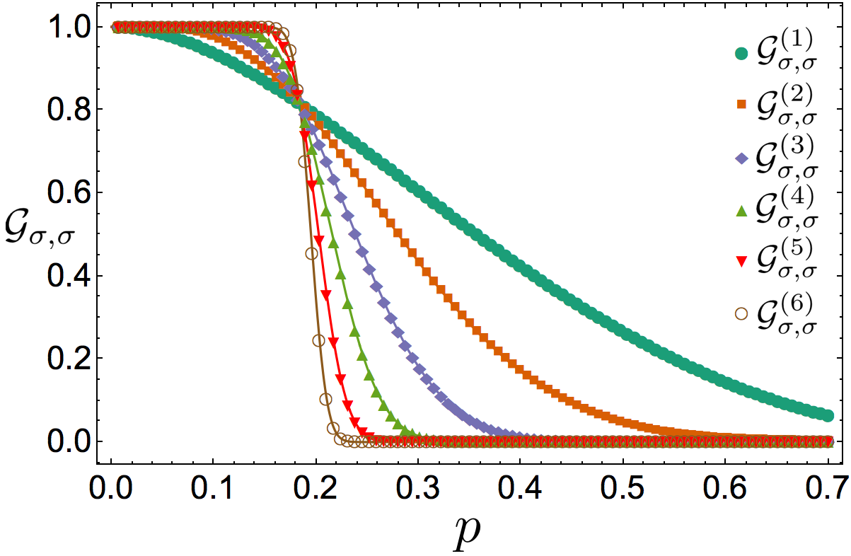
Figure 1: Representative plot of the smallest diagonal component $\bm{\mathcal{G}}_{\sigma,\sigma}$ of the process matrix for a noise model parametrized by $p$. As functions of $p$, the diagonal components of the process matrix approach a step-function as the number of concatenation levels approaches infinity. The threshold is the smallest value $p_{th}$ such that $\lim_{t\to\infty}\bm{\mathcal{G}}^{(t)}(\mathcal{N}_{p})=I_{4}$ for all $p\leq p_{th}$.

II.7 Specific decoders

The effective noise acting on a logical qubit is highly dependent upon both the physical noise processes and the choice of recovery operators for each syndrome (cf. eq. 24).

One decoder that will be very useful is the symmetric decoder; this decoder associates the measured syndrome with the error that acts on the fewest number of qubits and is consistent with the syndrome. If multiple errors acting on equal numbers of qubits are consistent with a syndrome, one is chosen arbitrarily and used each time that syndrome occurs. However the particular choice could affect the threshold value.

The symmetric decoder for the $[\![5,1,3]\!]$ code, for example, associates each syndrome to a unique weight-one Pauli operator. Therefore, all weight-one Pauli operators are corrected. However, one could choose a different decoder for the 5-qubit code. If we consider a noise model where only $X$-errors occur, a decoder could be chosen which corrects all weight-one and weight-two Pauli $X$ errors. However, this decoder would not be able to correct any $Y$ or $Z$ type Pauli errors. More details will be provided in sections V and VI.

III Hard decoding algorithm for optimizing error-correcting codes

We now present our optimized hard decoding algorithm that determines the choice of recovery operators at each level of concatenation. The goal of the algorithm is to correct the effective noise, that is, to map it to the identity channel $\mathcal{I}$ as quickly as possible. More formally, let $\epsilon$ be a pre-metric on the space of CPTP maps, that is, a function such that $\epsilon(\mathcal{N},\mathcal{M})\geq 0$ with equality if and only if $\mathcal{N}=\mathcal{M}$ and $\epsilon(\mathcal{N},\mathcal{M})=\epsilon(\mathcal{M},\mathcal{N})$ for all CPTP maps $\mathcal{N}$ and $\mathcal{M}$ (this is a pre-metric as $\epsilon$ does not have to satisfy the triangle inequality). The function $\epsilon(\mathcal{N}):=\epsilon(\mathcal{N},\mathcal{I})$ defines an ‘error rate’.

We will set $1-\epsilon(\mathcal{N})$ to be the average gate fidelity to the identity, defined in section III.1. This choice significantly reduces the amount of computational resources required to find the optimal recovery maps. The choice of $\epsilon$ may affect the performance of the decoder, however, we defer an investigation of this to future work.

Our hard decoding optimization algorithm selects recovery operations with the goal of minimizing the logical error rate after the recovery operations have been applied. The flowchart given in fig. 2 applies the hard decoding algorithm to a channel $\mathcal{N}$ and determines whether the effective noise will converge to the identity with concatenation. In fig. 2, $\mathcal{M}$ is a general CPTP map, $\mathcal{R}_{sym}$ is a (not necessarily unique) set of recovery operators for symmetric decoding (see section II.7), $\bm{\mathcal{G}}(\mathcal{M},k)$ are the distinct elements of $\{\bm{\mathcal{G}}(\mathcal{M},R):R\in\mathcal{R}_{sym}\}$, $m(k)$ is the number of instances of $\bm{\mathcal{G}}(\mathcal{M},k)$, and $L_{g}$ is a set of transversal logical operators. The optimized physical recovery maps are

$$R\to T(L_{g}^{\dagger})R$$ (36)

or all $R\in\mathcal{R}_{sym}$, where $g=m(k)\mathcal{G}(\mathcal{M},R)$ and $T(L_{g}^{\dagger})$ denotes the transversal implementation of $L_{g}^{\dagger}$. As we discuss in section IV, the choice for $L_{g}^{\dagger}$ may not be unique. The action of eq. 36 is equivalent to finding the set $\bm{\mathcal{L}}_{g}=\{L_{g}\thinspace:\thinspace g\in\mathscr{G}(\mathcal{M})\}$ of transversal logical operators that minimize

$$\epsilon(\sum_{g\in\mathscr{G}(\mathcal{M})}\bm{\mathcal{L}}_{g}g)$$ (37)

Figure 2: Method for selection of recovery operations for a fixed code $C$ and noise channel $\mathcal{N}$. The iterative step that calculates the process matrix at level $t$, $\mathcal{G}^{(t)}(\mathcal{N})$, is equivalent to setting the recovery maps to $R_{opt}=T(L_{g}^{\dagger})R$ for all $R\in\mathcal{R}_{sym}$, where $m(k)\bm{\mathcal{G}}(\mathcal{M},R)=g$ and $T(L_{g}^{\dagger})$ denotes the transversal implementation of $L_{g}^{\dagger}$. This set may not be unique; see section III.2 for specific examples of when this can occur. We use the $l_{\infty}$ norm, that is, the maximum of the absolute values of the entries of a matrix, to test whether the process matrix has converged. However, any matrix norm can be used instead.

There are $2^{n-1}$ syndromes, however, step 2 produces only 4, 7, 12, and 67 distinct process matrices for the $[\![5,1,3]\!]$, Steane, Shor, and surface-17 codes respectively, independently of the physical noise model. Therefore considering only the distinct $\bm{\mathcal{G}}(\mathcal{M},k)$ in step 2 reduces the memory and computational requirements by a factor between 4 and 20 for the codes considered in this paper. We could also improve performance by setting the off-diagonal terms to zero when they are sufficiently small and recalculating $\mathscr{G}(\mathcal{M})$ for Pauli channels $\mathcal{M}$. Removing the off-diagonal terms corresponds to performing a Pauli twirl by applying a uniformly-random Pauli operator $P$ to each physical qubit before the noise acts and then applying a logical $P$ at the $t^{\mathrm{th}}$ concatenation level. However, this step complicates the algorithm and was not necessary to obtain the results of this paper (it typically sped up computations by a factor between 2 and 10).

As we will discuss in section VIII, the use of a code’s non-Pauli transversal gates (note that for any stabilizer code the logical Pauli operators are always transversal) can significantly increase performance. This improvement is obtained when a syndrome measurement results in a logical non-Pauli error with high probability, which can occur even when significantly below threshold. This suggests that using highly symmetric stabilizer codes may provide better performance even at low error rates (in addition to also making non-trivial fault-tolerant computations more viable).

The resources required to find the set of recovery maps which optimally correct a noise model $\mathcal{N}$ are efficient in the number of concatenation levels required because our algorithm is independent of the observed syndromes from previous concatenation levels. The largest contribution to the complexity of our scheme comes from computing the $\beta$ matrix for each syndrome measurement. From eq. 22, there are $3\times 2^{n-1}$ operations required to compute a $\beta$ matrix for a particular syndrome value. The factor of 3 comes from computing the commutation relations (encoded by $\eta$) between $R_{l}$ and the code’s logical Pauli operators ($R_{l}$ always commutes with the identity) and the factor of $2^{n-1}$ comes from verifying the commutation relations between $R_{l}$ and all elements in the stabilizer group. As there are $2^{n-1}$ possible syndrome values, $3\times 2^{2(n-1)}$ operations are required to compute all the $\beta$ matrices.

III.1 Infidelity-optimized decoding

The average gate infidelity to the identity (hereafter simply the infidelity),

$$r(\mathcal{N})=1-\int\mathrm{d}\psi\langle\psi|\mathcal{N}(|\psi\rangle\!\langle\psi|)|\psi\rangle,$$ (38)

is a commonly-used error pre-metric on the space of CPTP maps where the integral is over all pure states according to the unitarily-invariant Fubini-Study metric. The infidelity can be written as

$$r(\mathcal{N})=\frac{4-\operatorname{\mathrm{Tr}}\bm{\mathcal{N}}}{6}$$ (39)

in the process matrix formalism for a single qubit Kimmel et al. (2014). The infidelity is particularly convenient for our algorithm because the trace is a linear function of the channel. Consequently, to find a set $\{L_{g}:g\in\mathscr{G}(\mathcal{M})\}$ that minimizes $\epsilon\Bigl{(}\sum_{g\in\mathscr{G}(\mathcal{M})}\bm{\mathcal{L}_{g}}g\Bigl{)}$ it is sufficient to maximize

$$\operatorname{\mathrm{Tr}}\bm{\mathcal{L}}g$$ (40)

independently for each $g\in\mathscr{G}(\mathcal{M})$, rather than considering all $\lvert\mathscr{G}(\mathcal{M})\rvert^{\lvert\mathscr{L}\rvert}$ possibilities.

III.2 Resolving ties

There is one important caveat in the implementation of our hard decoding algorithm, namely, there may be multiple sets $\{L_{g}:g\in\mathscr{G}(\mathcal{M})\}$ that minimize the error in $\epsilon\Bigl{(}\sum_{g\in\mathscr{G}(\mathcal{M})}\bm{\mathcal{L}_{g}}g\Bigl{)}$.

For example, consider the Steane code with $\mathcal{U}_{\theta}(\rho)=U_{\theta}\rho U_{\theta}^{\dagger}$ and $U_{\theta}=\cos\theta I_{2}+i\sin\theta X$. Then the only two matrices from step 2 of our algorithm for any value of $\theta\in[-\tfrac{\pi}{4},\tfrac{\pi}{4}]$ are

$$\bm{\mathcal{R}}_{z1}(\theta) =\frac{7\cos(8\theta)+25}{32}\bm{\mathcal{U}_{\phi/2}}$$

$$\bm{\mathcal{R}}_{z2}(\theta) =\frac{7\sin^{2}(4\theta)}{16}\bm{\mathcal{U}}_{-3\theta}$$ (41)

for the trivial syndrome and the syndromes that detect $X$ errors respectively, where

$$\phi =\arctan\Bigl{(}\frac{(3\cos(4\theta)+\cos(8\theta)+10)\tan^{3}(2\theta)}{-3\cos(4\theta)+\cos(8\theta)+10}\Bigr{)}$$

$$=14(\theta^{3}+\theta^{5})+O(\theta^{7}).$$ (42)

Similar expressions hold for other values of $\theta$ with different signs.

For this example, using all transversal gates significantly improves the recovery, as, for example, $U_{\pm\pi/4}$ (the phase gate around the $X$-axis) is a transversal gate and so $\bm{\mathcal{R}}_{z2}(\pi/12)$ can be perfectly recovered. Furthermore, there are two logical gates, namely $U_{0}$ and $U_{\pi/4}$, that maximize eq. 40 for $g=\bm{\mathcal{R}}_{z2}(\pi/24)$, and so the choice is ambiguous. When confronted with such ambiguities, we choose the first logical operator that maximizes eq. 40 (in particular, the identity if it is one of the options). As we will discuss further in section V, this ambiguity due to the ordering of logical operators does arise in practical examples without “fine-tuning” any parameters and it can impact performance.

IV Numerically calculating threshold hypersurfaces

We now describe our numerical method for calculating threshold hypersurfaces under symmetric (section II.7) and infidelity-optimized decoders (section III). For convenience, we regard a noise channel $\mathcal{N}$ as correctable if there exists some level of concatenation $t$ such that $\operatorname{\mathrm{Tr}}\bm{\mathcal{G}}^{(t)}\geq 4-\xi$, or, equivalently, the infidelity of $\mathcal{\bm{G}}^{(t)}$ is at most $\xi/6$. The value of $\xi$ was set to 0.01.

Figure 3: Method for lower-bounding the threshold for a one-parameter noise model $\mathcal{N}_{p}$, where $t(p)$ is the minimum number of concatenation levels required to correct $\mathcal{N}_{p}$. We begin by setting $p_{in}=p_{sym,thres}$ and $\delta p=0.01$, then repeating with the new lower bound and $\delta p=0.001$ and finally $\delta p=0.0001$. To find the threshold hypersurface for an $m$-parameter noise model, repeat this procedure for $\mathcal{N}_{pq}$ while iterating through a mesh of points, $q$.

IV.1 Symmetric threshold hypersurfaces

The subset of correctable errors for a given noise model is not generically connected. For this reason, a binary search between $p=0$ and $p=1$, where $p$ is the noise parameter, is insufficient when calculating a threshold value because this method may miss some uncorrectable regimes. To calculate $p_{sym,thr}(q)$, a threshold value of $p$ (with $q$ fixed) when a symmetric decoder is applied at each level of concatenation, we initialized $p=0$ and incremented by 0.05 until the noise with $p=p_{u}$ was uncorrectable, then implemented a binary search between $p=p_{u}-0.05$ and $p=p_{u}$. To find a threshold hypersurface for a noise model with multiple parameters, we iteratively apply this procedure while varying $q$ over a dense mesh.

IV.2 Threshold hypersurfaces for our infidelity-optimized decoder

To calculate threshold values of a code $C$ afflicted by a general CPTP map using our hard decoding algorithm, we follow the procedure illustrated in fig. 3. Here $t(p)$ is the minimum number of concatenation levels required to correct $\mathcal{N}_{pq}$.

V Thresholds and infidelities for amplitude-phase damping

In the remainder of the paper, we show that our hard decoding algorithm leads to significant improvements in threshold values and, in some cases, decreases the infidelity by several orders of magnitude relative to the symmetric decoder. We will also show that the performance of our decoder is robust to perturbations in the noise, so that it can be implemented using the necessarily imperfect knowledge of the noise in an experiment.

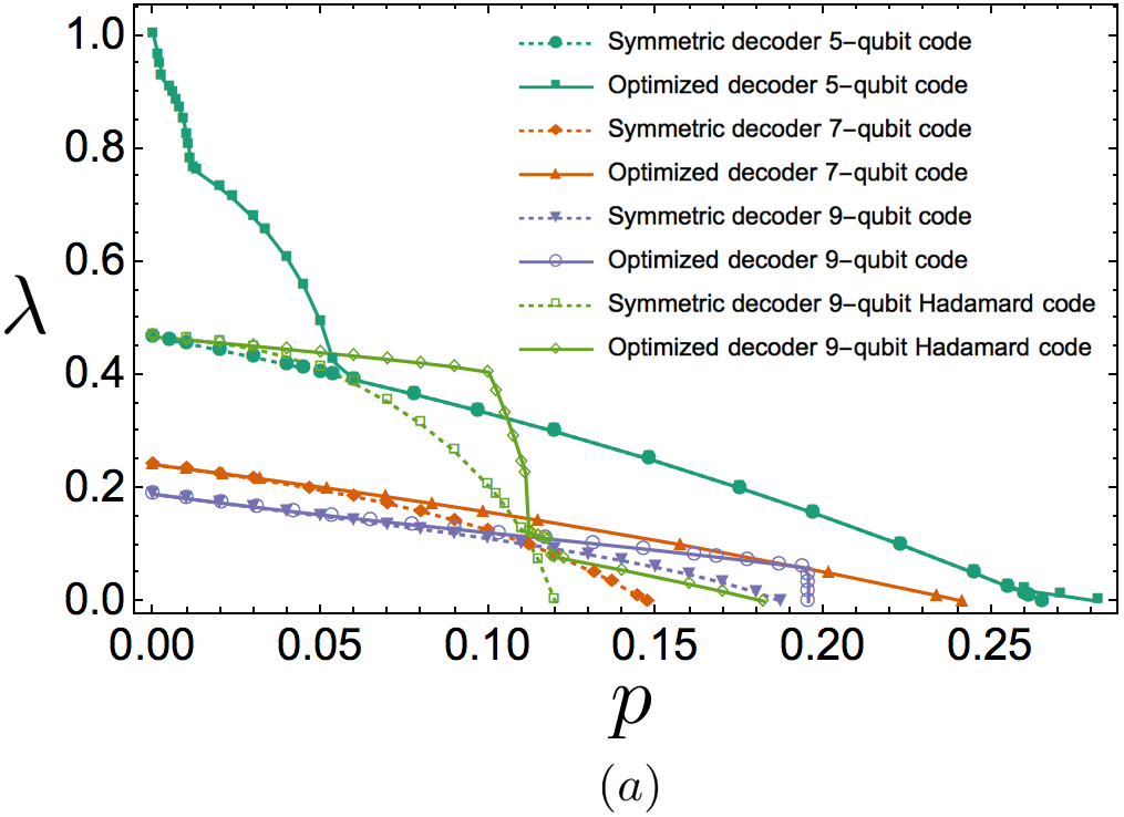
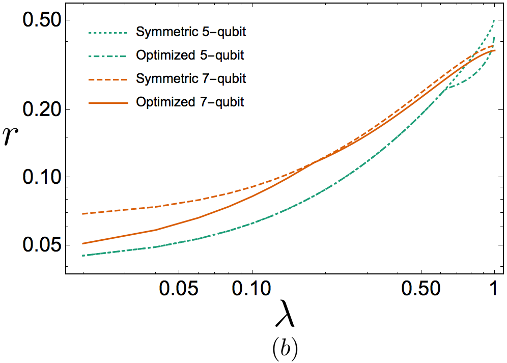
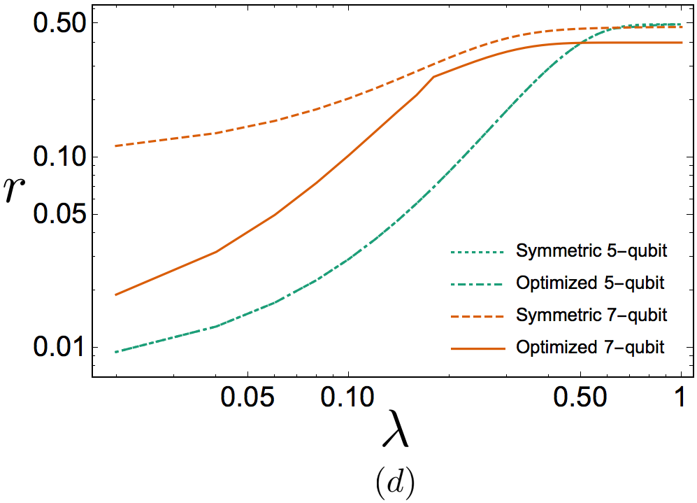
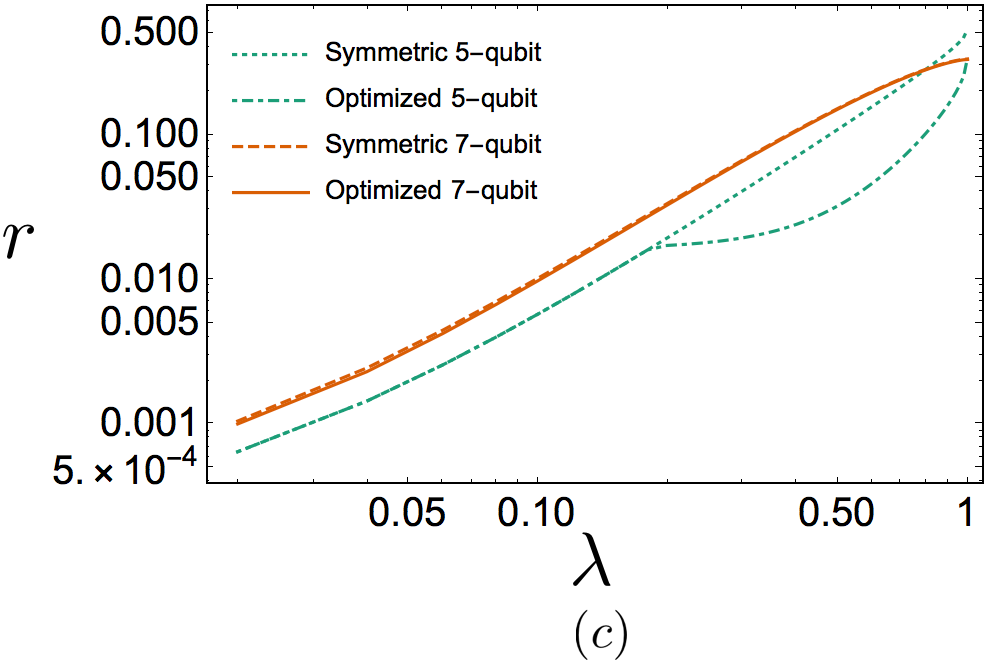
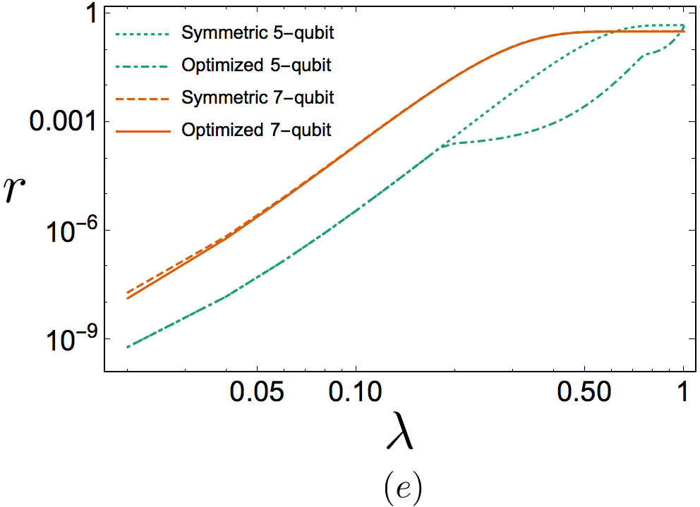
Figure 4: Threshold curves (a) and infidelities $r$ as functions of the dephasing parameter $\lambda$ at the first (b), (c) and third (d), (e) concatenation level for the amplitude-phase damping channel under the $[\![5,1,3]\!]$ and Steane codes. The Shor and surface-17 codes behave similarly to the Steane code and so their infidelity curves are not displayed. Our numerics also show that for small $p$, the 5 and $X$-Shor codes have the highest thresholds due to lowest number of qubits and asymmetry of stabilizers matching the asymmetry of the noise. The amplitude damping rate is fixed at $p=0.17$ (b), (d) and $p=0.01$ (c), (e). The symmetrized and optimized curves overlap when the optimized decoder is the symmetric decoder, however, there are many regimes where the optimized decoder improves the threshold and infidelity. For the $[\![5,1,3]\!]$ code, thresholds using the optimized decoder increase by as much as a factor of 2.14 relative to the symmetric decoder. Infidelities are lowered by as much as 2 orders of magnitude. The curves for the fixed symmetric decoders are all smooth, whereas the curves for the optimized decoders have kinks corresponding to points where the decoder changes to exploit asymmetries in the noise. When $\lambda$ is large compared to $p$, the noise is primarily dephasing. The $[\![5,1,3]\!]$ code can exploit this by correcting all single- and two-qubit $Z$ errors for the first $t$ concatenation levels, until the noise becomes unbiased (the kink in (b) corresponds to $t=1$, and the two in (c) correspond to $t=2,3$). The $X$-Shor code can also be biased to correct Pauli-$Z$ errors as it has more $X$-type stabilizers. All codes also exhibit improved performance for large values of $p$ relative to $\lambda$, that is, when the noise is primarily amplitude damping.

In this section we consider a physical noise model consisting of both amplitude and phase damping processes. The amplitude damping channel acts on a two-level system at zero temperature. If the system is in the excited state, then a transition to the ground state occurs with probability $p$. If the system starts in the ground state, it will remain in the ground state indefinitely. A physical example of this scenario would be the spontaneous emission of a photon in a two-level atom. The Kraus operators for the amplitude damping channel are Nielsen and Chuang (2000)

$$A^{(0)}_{AD}=\left(\begin{array}[]{cc}1&0\\ 0&\sqrt{1-p}\\ \end{array}\right),\hskip 2.84544ptA^{(1)}_{AD}=\left(\begin{array}[]{cc}0&\sqrt{p}\\ 0&0\\ \end{array}\right).$$ (47)

We point out that eq. 47 can be generalized to take into account non-zero temperature effects. In this case, when the system is in the ground state, there is a non-zero probability of making a transition to the excited state. In Cafaro and van Loock (2016), the performance of the 5-qubit code, Steane code and non-additive quantum codes was estimated for the generalized amplitude damping channel. However, the methods used did not allow for an exact analysis. In the remainder of this manuscript we will only consider the amplitude-damping channel at zero temperature.

Phase damping arises when a phase kick $\exp(i\theta Z)$ is applied to a qubit with a random angle $\theta$. When $\theta$ is sampled from a Gaussian distribution, then the Kraus operators are

$$A^{(0)}_{PD}=\left(\begin{array}[]{cc}1&0\\ 0&\sqrt{1-\lambda}\\ \end{array}\right),\hskip 2.84544ptA^{(1)}_{PD}=\left(\begin{array}[]{cc}0&0\\ 0&\sqrt{\lambda}\\ \end{array}\right),$$ (52)

where $\lambda$ characterizes the width of the distribution of $\theta$. The phase damping channel is also equivalent to the phase-flip channel, that is, applying a $Z$ with probability $\alpha=(1+\sqrt{1-\lambda})/2$.

Combining the amplitude and phase damping channel, we consider the amplitude-phase damping channel given by

$$\mathcal{N}_{APD}(\rho)=\mathcal{N}_{PD}(\mathcal{N}_{AD}(\rho))=\mathcal{N}_{AD}(\mathcal{N}_{PD}(\rho)).$$ (53)

As the amplitude-phase damping channel contains two parameters ($p$ and $\lambda$), the threshold hypersurface will be a curve below which the process matrix is correctable.

The threshold curves and infidelity at the first and third concatenation levels for the $[\![5,1,3]\!]$, Steane, and Shor codes are illustrated in fig. 4. The infidelities for the Shor and surface-17 codes are not shown since they behave similarly to the Steane code. The $[\![5,1,3]\!]$ code generally outperforms all other codes in terms of logical infidelity and thresholds under both optimized and symmetric decoders, except in an intermediate regime where the optimized decoder exploits the asymmetry in the stabilizers of the $X$-Shor code.

The optimized decoder coincides with the symmetric decoder for each code in some parameter regimes, although only when $p=0$ for the Steane and Shor codes. However, the optimized decoder often differs significantly from the symmetric decoder, resulting in substantially improved logical infidelities and thresholds. The optimized decoder changes in different parameter regimes to exploit asymmetries in the noise, producing the kinks in the curves in fig. 4. The amplitude-phase damping channel is highly biased towards $Z$ errors for small values of $p$ relative to $\lambda$. The optimized decoder exploits this for the $[\![5,1,3]\!]$ code by only correcting $Z$ errors for $t$ levels of concatenation until the noise is approximately symmetric, and then switching to the symmetric decoder, with $t$ increasing as $p$ approaches zero. The $X$-Shor code also performs better in this regime as it has more $X$-type stabilizers that detect $Z$-type errors.

The optimized decoder also results in improved thresholds and logical infidelities for high amplitude damping rates for all codes. The noise is significantly different from Pauli noise in this regime and so decoders constructed under the assumption of Pauli noise will be less likely to identify the correct error compared to decoders optimized for amplitude-phase damping.

As discussed in section III.2, multiple sets $\{L_{g}:g\in\mathscr{G}(\mathcal{M})\}$ maximize eq. 40 for the Steane code with amplitude-phase damping and large values of $\lambda$. For example, setting $\lambda=0.1431$ and choosing the first recovery operator that maximizes eq. 40 gives a threshold of $p_{th}=0.1032$. However, searching all tuples $\{L_{g}:g\in\mathscr{G}(\mathcal{M})\}$ that maximize eq. 40 (where the degeneracy only occurs at the first level) for the same value of $\lambda$ gives a higher threshold of $p_{th}=0.1150$.

VI Thresholds for coherent errors

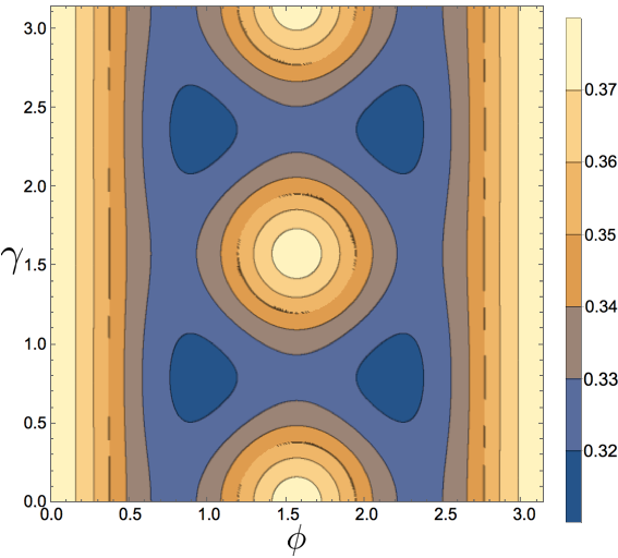
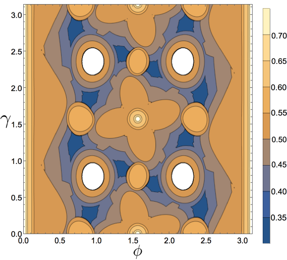
(a)

(b)

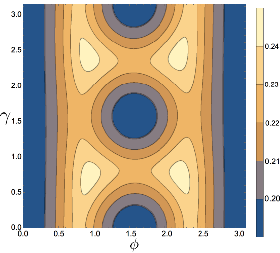
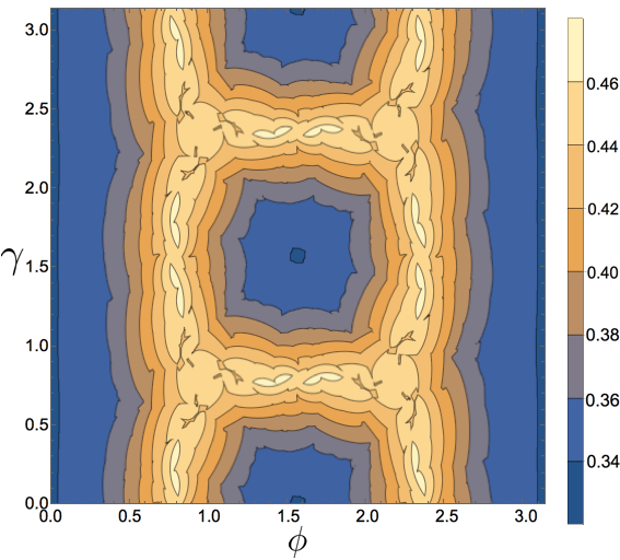
(c)

(d)

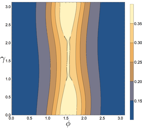
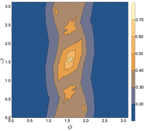
(e)

(f)

Figure 5: Contour plots representing hypersurfaces of the threshold value of $\theta$ for rotations around the axis $\hat{n}=(\sin\phi\cos\gamma,\sin\phi\sin\gamma,\cos\phi)$ for (a) the $[\![5,1,3]\!]$ code, (c) the Steane code and (e) the Shor code using the symmetric decoder and (b) the $[\![5,1,3]\!]$ code, (d) the Steane code and (f) the Shor code using optimized decoding. The optimized decoder uses transversal gates to improve the threshold, particularly when the rotation is around an eigenbasis of a transversal Clifford gate (see table 1). In particular, the $[\![5,1,3]\!]$ code has a transversal $\pi/3$ rotation around $\hat{n}_{C}=(1,1,1)/\sqrt{3}$ (i.e., $\gamma=\pi/4$, $\phi=\pi/3$), which enables the optimized decoder to correct arbitrary rotations around axes close to $\hat{n}_{C}$, illustrated by the white circular regions in (b). For Steane’s code, the lightest colored regions in (d) corresponds to threshold angles $\theta_{th}\approx 0.46$ compared to $\theta_{th}\approx 0.24$ in (c), an improvement by almost a factor of 2. The Shor code has no transversal non-Pauli gates and so the improvements from the optimized decoder are not as substantial. However, for rotations near the $y$-axis, the Shor code outperforms the Steane code by a factor of at most 2.3.

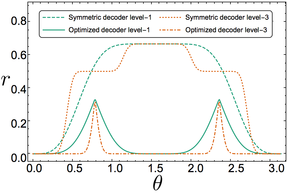
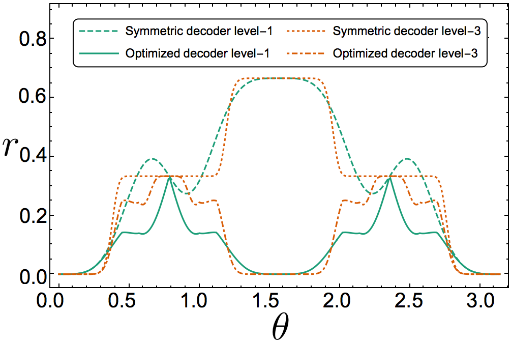
(a)

(b)

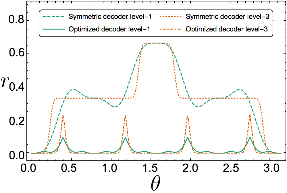
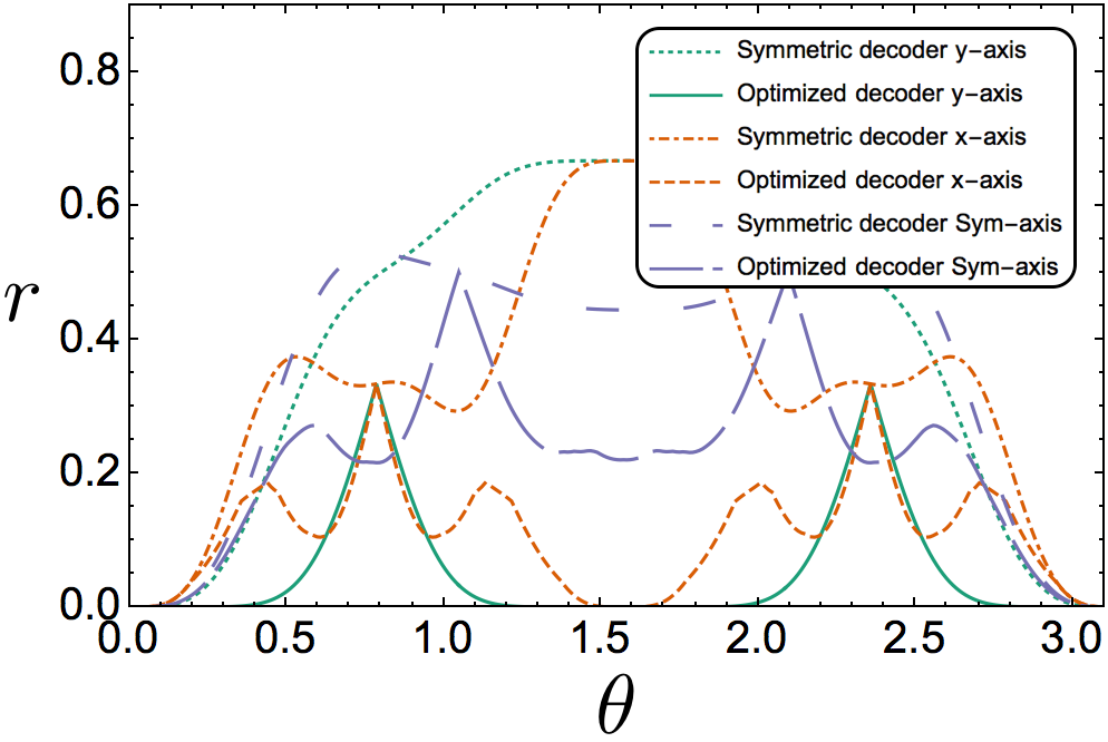
(c)

(d)

Figure 6: In (a), (b) and (c) infidelities $r$ of the $[\![5,1,3]\!]$ code, Shor code and Steane code are plotted at the first and third levels for a rotation about the $x$-axis. In (a), the optimized infidelity curves are peaked at the code’s threshold value $\theta_{th}=\pi/4$. In (b), the peaks of the optimized infidelity curves are centred slightly above the code’s threshold value $\theta_{th}=0.3396$. However, the optimized level-3 infidelity curve intersects the optimized level-1 curve at the threshold value as expected. In (c), the optimized level-1 and level-3 infidelity curves intersect at the threshold value $\theta_{th}=0.3692$. The peaks of the infidelity curves occur at $\theta=\pi/4$ due to the codes symmetry. In (d), infidelity plots of the surface-17 at the first concatenation level are shown for a rotation about the $y$-axis, $x$-axis and the $(1,1,1)/\sqrt{3}$ axis. It can be seen that the infidelity is lowest for rotations about the $y$-axis. In all 4 plots, it can be seen that applying our hard decoding algorithm reduces the infidelities by, in some cases, orders of magnitude compared to the symmetric decoder.

In this section we illustrate the behavior of coherent errors under error correction. We consider a coherent error noise model where every qubit undergoes a rotation by an unknown angle $\theta$ about an axis of rotation $\hat{n}$. The coherent noise channel can thus be written as

$$\mathcal{N}_{\theta,\phi,\gamma}(\rho)=e^{i\theta\hat{n}\cdot\vec{\sigma}}\rho e^{-i\theta\hat{n}\cdot\vec{\sigma}},$$ (54)

where $\hat{n}=(\sin\phi\cos\gamma,\sin\phi\sin\gamma,\cos\phi)$. We obtain the threshold hypersurface for the noise model

$$\mathscr{N}=\{\mathcal{N}_{\theta,\phi,\gamma}:\theta\in[0,2\pi],\gamma,\phi\in[0,\pi]\},$$ (55)

by fixing $\gamma$ and $\phi$ and obtaining the threshold for $\theta$.

The threshold hypersurfaces for the $[\![5,1,3]\!]$, Steane, and Shor codes are illustrated as contour plots in fig. 5. The infidelities at the first and third concatenation levels for $[\![5,1,3]\!]$, Steane, Shor, and surface-17 (1st level only) codes are plotted in fig. 6.

Unlike with amplitude-phase damping noise, the optimized decoder strictly outperforms the symmetric decoder for all rotation axes. With the exception of the Shor code, the threshold hypersurfaces are relatively flat under symmetric decoding, that is, the threshold rotation angle is relatively independent of the rotation axis. The optimized decoder breaks this, giving larger threshold angles for different axes, particularly for rotations about an eigenbasis of the transversal Clifford gates listed in table 1. In particular, the $[\![5,1,3]\!]$ code can correct any rotation about axes $\hat{n}$ that are close to $(\pm,\pm,\pm)/\sqrt{3}$. The Steane code can correct any rotation about the Pauli axes except for angles close to odd integer multiples of $\pi/4$. The performance of the Shor code is generally only modestly improved by the optimized decoder, largely because the Shor code has no transversal non-Pauli gates. However, the optimized decoder is able to exploit the asymmetries in the stabilizer generators to increase the threshold for rotations near the $y$ axis by more than a factor of 3.

The improved threshold angles are reflected in the orders-of-magnitude reduction in the logical infidelities in fig. 6. The infidelities are periodic because transversal gates can be used to counteract the unitary noise. However, as discussed in section VIII, the transversal gates are useful even when the action of the noise on the codespace is far from a transversal gate. For the $[\![5,1,3]\!]$, Steane and $Z$-Shor codes, the infidelities are the infidelity at the first and third concatenation levels for rotations about the $x$ axis, while for the surface-17 code the infidelities are at the first level for rotations about the $x$, $y$ and $\frac{1}{\sqrt{3}}(1,1,1)$ axes. For the $[\![5,1,3]\!]$, Steane and Shor codes, the threshold values of $\theta$ correspond exactly to the cross-over points between the level-1 and level-3 curves. At the third level, the infidelity is greatly suppressed below threshold and increased above threshold. The optimized infidelity curves are lower (in some cases by several orders of magnitude) than the infidelities arising by applying the symmetric decoder at all levels.

For the $[\![5,1,3]\!]$ code, the only uncorrectable values of $\theta$ are odd integer multiples of $\pi/4$. The surface-17 code has a higher threshold against $Y$ errors than against $X$ (or $Z$) errors. The surface-17 code treats $X$ and $Z$ errors symmetrically. However, since the $X$ and $Z$ stabilizer generators have support on different qubits, error rates resulting from $Y$ errors will differ from error rates resulting from $X$ and $Z$ errors.

The optimized decoding algorithm gives the greatest improvements for codes with transversal non-Pauli gates, namely, the $[\![5,1,3]\!]$ and Steane codes.

VII Correlated noise channel

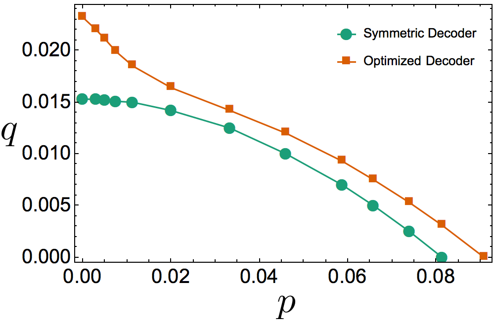
(a)

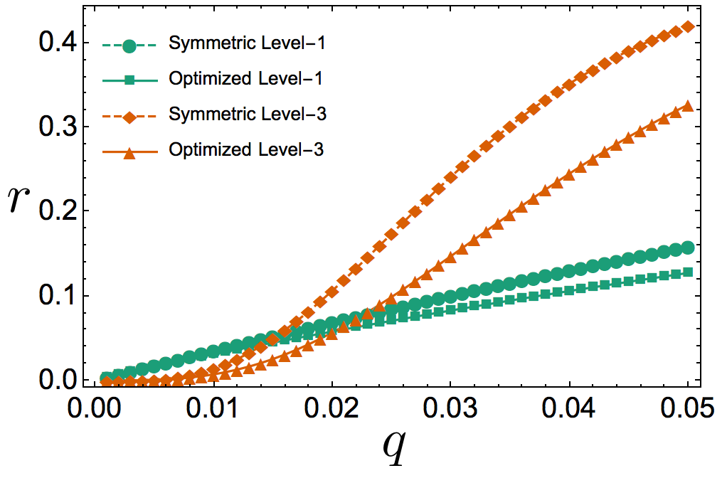
(b)

Figure 7: (a) Threshold curves and (b) infidelities $r$ at the first and third concatenation level (with fixed $p=0.003$) for the $[\![7,1,3]\!]$ code. Two-qubit correlated dephasing occurs with probability $q$ and depolarizing noise occurs with probability $1-q$, with a depolarizing noise parameter $p$ (see eqs. 56 and 57). For small values of $p$, the $Z$ errors arising from the two-qubit correlations dominate the noise. Applying our optimized hard decoding algorithm in this regime yields a threshold of $q_{th}=0.0232$. The contribution from depolarizing noise increases with $p$ until the noise is predominantly depolarizing. In this regime, the optimized decoder implements the standard CSS decoder at all levels. When $q=0$, the noise is purely depolarizing and $p_{th}=0.0908$. For all values of $p$, the threshold $q_{th}$ obtained by implementing our optimized decoder is larger than the threshold obtained by implementing the symmetric decoder. The level-1 and level-3 infidelity curves intersect near the respective thresholds for $p=0.003$, namely, $q_{th}=0.0153$ and $q_{th}=0.0220$ for the symmetric and optimized decoders respectively.

In this section, we study the effect of correlated noise on the logical noise in Steane’s code. The correlated noise we consider consists of local depolarizing noise and two-qubit correlated dephasing errors to all adjacent pairs. The composite noise channel maps an $n$-qubit state $\rho$

$$\mathcal{N}(\rho)=(1-q)\mathcal{D}_{p}^{\otimes n}(\rho)+\frac{q}{n}\sum_{j=1}^{n}\mathcal{Z}_{j,j+_{n}1}^{(2)}(\rho),$$ (56)

where $j+_{n}1=j+1$ if $j<n$ and $1$ otherwise (that is, we consider the qubits to be in a ring),

$$\mathcal{D}_{p}(\tau)=(1-p)\tau+\frac{p}{3}(X\tau X+Y\tau Y+Z\tau Z)$$ (57)

is the depolarizing channel acting on a single-qubit state $\tau$, and $\mathcal{Z}_{j,j+_{n}1}(\rho)=Z_{j}Z_{j+1}\rho Z_{j+1}Z_{j}$ applies phase-flip operators to qubits $j$ and $j+1$. The logical process matrix can be computed for the noise model in eq. 56 by eq. 27.

The threshold and infidelity at the first and third concatenation levels of Steane’s code are illustrated in fig. 7. In the small $p$ regime, the noise is dominated by the two-qubit correlated dephasing contribution. The optimized decoder corrects a larger amount of $Z$ errors at the first few levels by breaking the symmetry in the syndrome measurements. At higher levels, the decoder corrects in a more symmetric fashion in order to remove the remaining Pauli errors. This improved performance is also illustrated in the reduced optimized logical infidelities shown in fig. 7 (b) as a function of $q$ with $p=0.003$.

There is an intermediate regime where the local depolarizing noise contribution becomes more relevant, leading to a decrease in the threshold value for $q$. However, the optimized threshold is still noticeably larger than the symmetric decoder threshold. Finally, when the local depolarizing noise is the dominant source of noise, our optimization algorithm chooses recovery maps consistent with the standard CSS decoder. The standard CSS decoder yields a slightly larger $p$ threshold value compared to the symmetric decoder when $q=0$.

VIII The effect of Pauli twirling on thresholds and the benefits of using transversal operations

In sections V, VII and VI, we showed that our hard decoding optimization algorithm could improve threshold values by more than a factor of 2 for amplitude-phase damping noise. For coherent noise there where certain rotation axes where the noise was correctable for arbitrary rotation angles. Infidelities were reduced by orders of magnitudes in certain regimes. The amplitude-phase damping and coherent noise models are both non-Pauli. Performing a Pauli twirl on a noise channel $\mathcal{N}$ (that is, conjugating it by a uniformly random Pauli channel) maps it to a channel $\mathcal{T}(\mathcal{N})$ that is a Pauli channel and so has a diagonal matrix representation with respect to the Pauli basis Emerson et al. (2007); Geller and Zhou (2013). In Geller and Zhou (2013); Gutiérrez et al. (2016), the effective noise at the first level for the amplitude damping channel was found to be in good agreement to a Pauli twirled approximation of the channel.

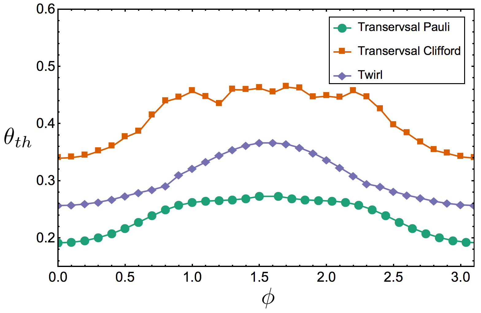
Figure 8: Threshold curves for unitary rotations about $(\tfrac{1}{\sqrt{2}}\sin\phi,\tfrac{1}{\sqrt{2}}\sin\phi,\cos\phi)$ by an angle $\theta$ under three different decoding schemes for the Steane code. For all values of $\phi$, an improvement by as much as a factor of 1.7 in the threshold $\theta_{th}$ obtained by using our algorithm optimizing over all transversal Clifford gates can be observed relative to optimizing over all Pauli gates. The Pauli-twirl reduces (increases) the threshold when optimizing over all transversal Clifford (Pauli) gates for all values of $\phi$.

However, we now show that performing a Pauli twirl on coherent noise and using the Steane code can either reduce or increase threshold values, depending on the particular recovery protocol. We also illustrate the improvements obtained by using all transversal gates in the decoding algorithm, instead of just the Pauli gates. Threshold curves for rotations about $(\tfrac{1}{\sqrt{2}}\sin\phi,\tfrac{1}{\sqrt{2}}\sin\phi,\cos\phi)$ by an angle $\theta$ under three different decoding schemes for the Steane code are presented in fig. 8. The three schemes we consider are : 1) our optimized decoding algorithm applied to the twirled noise; 2) our optimized decoding algorithm applied to the bare noise using all transversal gates; and 3) our optimized decoding algorithm applied to the bare noise using only transversal Pauli gates. Using transversal Clifford gates in our recovery protocol gives the largest threshold values for all values of $\phi$ and so Pauli twirling reduces the threshold. However, if only transversal Pauli operators are used, Pauli twirling increases the threshold for all values of $\phi$.

The curves in fig. 8 also demonstrate that the threshold can increase by at most a factor of 1.7 when optimizing over all transversal gates for coherent noise compared to optimizing over all transversal gates for the twirled channel. This advantage arises for two reasons. First, for a known noise model, a transversal gate can be applied to map it to another noise model that may be closer to the identity. Second, syndrome measurements may map coherent errors closer to a non-Pauli unitary. However, both these benefits are lost when the noise is twirled because both the physical noise and the noise for each syndrome is Pauli noise, which is generally far from any non-Pauli unitary.

IX Sensitivity and robustness of our hard decoding optimization algorithm to perturbations of the noise model

In section III, we presented a hard decoding algorithm for optimizing threshold values of an error correcting code for arbitrary CPTP maps. Our algorithm can therefore be applied to non-Pauli channels, including more realistic noise models that could be present in current experiments. However, the noise afflicting an experimental system is only ever approximately known. Nevertheless, we now demonstrate that applying the decoder obtained by our algorithm for a fixed noise channel $\mathcal{N}$ to a perturbed noise model $\mathcal{N}_{p}$ retains, in some cases, improvements in error suppression relative to the symmetric decoder.

To study perturbations about a noise channel, let $\mathscr{N}=\{\mathcal{N}_{p}:p\in[0,1]\}$ be a 1-parameter noise model and

$$\mathcal{N}_{U,p}(\rho)=[1-f(p)]\mathcal{N}_{p}+f(p)U\rho U^{\dagger}$$ (58)

where $U$ is a random unitary and $f:[0,1]\to[0,1]$ is a function such that $f(p)\ll\lVert\mathcal{N}_{p}-\mathcal{I}\rVert$ for any suitable norm (e.g., the diamond norm). (The generalization to multi-parameter noise families is straightforward.)

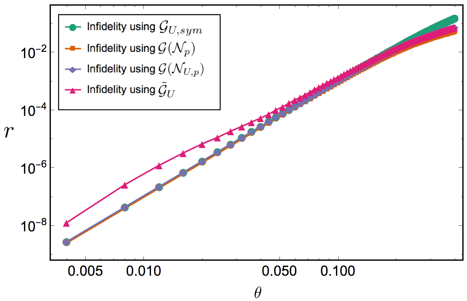
(a)

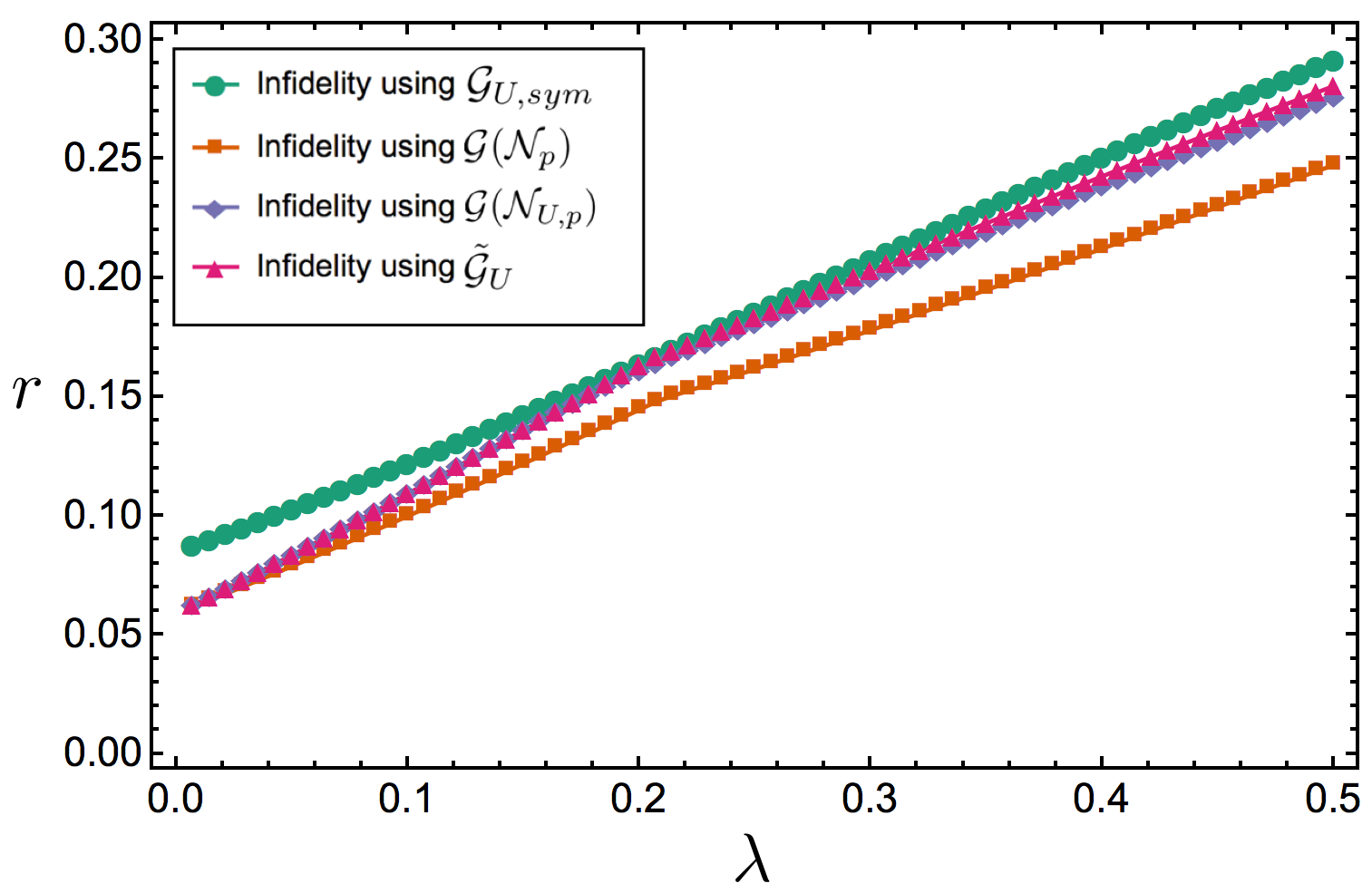
(b)

Figure 9: Averaged infidelity plots over 100 random unitary operators $U$ of the effective process matrices $\mathcal{G}(\mathcal{N}_{p})$, $\mathcal{G}(\mathcal{N}_{U,p})$, $\mathcal{G}_{U,sym}$ and $\tilde{\mathcal{G}}_{U}$. The figure in (a) is obtained using the $[\![5,1,3]\!]$ code for coherent errors using random rotation axes for each random unitary. The perturbation was chosen to have the form $f(\theta)=\sin^{2}{\theta}/10$. The figure in (b) is obtained using the Steane code for the amplitude-phase damping channel. The perturbation was chosen to have the form $f(\lambda)=\lambda/10$. In (a), the inset plot shows all infidelities on a log-log scale in the regime where $\theta$ is small. As can be seen from the figure, in the regime where $\theta\gtrsim 0.185$, the optimized recovery maps for the unperturbed channel yield a lower infidelity when applied to the perturbed channel than that from applying the symmetric decoder. For smaller rotation angles, the infidelity from $\tilde{\mathcal{G}}_{U}$ is slightly larger than the infidelity arising from $\mathcal{G}_{U,sym}$. The two differ by at most a factor of 7 in the small $\theta$ limit. The infidelity obtained by applying the hard decoding optimization algorithm to the unperturbed channel is lowest for all sampled values of $\theta$. In (b), it can be observed that applying the decoder chosen by our optimization algorithm for the unperturbed channel to the perturbed channel results in a lower infidelity than applying the symmetric decoder to the perturbed channel, for all sampled values of $\lambda$. This indicates that our decoding scheme is very robust to small perturbations of the amplitude-phase damping channel.

We applied our algorithm to $\mathcal{N}_{p}$ and $\mathcal{N}_{U,p}$, giving the effective process matrices $\mathcal{G}(\mathcal{N}_{p})$ and $\mathcal{G}(\mathcal{N}_{U,p})$ respectively. We then applied the symmetric decoder and the decoder optimized for $\mathcal{N}_{p}$ to the perturbed noise $\mathcal{N}_{U,p}$ to obtain the process matrices $\mathcal{G}_{U,sym}$ and $\tilde{\mathcal{G}}_{U}$ respectively. The infidelities of these process matrices (at the first concatenation level) are plotted in fig. 9 (a) for the $[\![5,1,3]\!]$ code with coherent noise and $f(\theta)=\sin^{2}\theta/10$ and in fig. 9 (b) for the Steane code with amplitude-phase damping, $p=0.2$ and $f(\lambda)=\lambda/10$. For both plots we averaged the values over 100 uniformly random unitaries. These results demonstrate that the significant improvements obtained using the optimized decoder are, in most studied cases, robust to perturbations in the noise.

The one exception we observed is for coherent noise in the $[\![5,1,3]\!]$ code for $\theta\lesssim 0.185$, where the infidelity obtained using the optimized decoder for the unperturbed channel is larger than that obtained using the symmetric decoder by a factor of at most 7.

X Conclusion

In this paper, we presented an optimized hard decoding algorithm for arbitrary local Markovian noise and numerical techniques to characterize thresholds for noise models. Block-wise two-qubit correlated noise was also considered. Using the analytical tools of section II, we provide numerical results in sections V, VI, VII, VIII and IX which shows substantial improvements obtained by our algorithms compared to a fixed decoder for a variety of noise models, including coherent errors, correlated dephasing and amplitude-phase damping, and codes, namely, the $[\![5,1,3]\!]$, Steane, Shor and surface-17 codes. For coherent noise, our optimized decoding algorithm allowed, in some cases, the noise to be corrected for all sampled rotation angles and reduced infidelities at a fixed concatenation level by orders of magnitude.

Our hard decoding algorithm is scalable and efficiently optimizes the recovery operations independently at each concatenation level while taking advantage of a code’s transversal gates. At a given concatenation level, all syndrome measurements are considered rather than being sampled from a distribution, so that the performance is exactly characterized rather than containing statistical (and state-dependent) uncertainties.

In contrast to hard decoding, message-passing algorithms Poulin (2006) can increase thresholds for Pauli noise, in some cases nearing the hashing bound subject to sampling uncertainties. Large codes can also be studied using tensor networks Darmawan and Poulin (2016), although this requires a tensor-network description of the code and is exponential in the code distance. An interesting and important open problem is to combine the current techniques with those of Refs. Poulin (2006); Darmawan and Poulin (2016) to either reduce statistical uncertainties in message-passing algorithms by exploiting symmetries in the code or to treat larger, non-concatenated code families.

Further, we showed that performing a Pauli twirl can increase or decrease the threshold depending on the code and noise properties. In Gutiérrez and Brown (2015), the Pauli twirl was found to have little impact on the performance of amplitude damping, which is known to be “close” to Pauli noise (that is, exhibit similar worst-case errors) Kueng et al. (2016). We conjecture that Pauli twirling will generally reduce thresholds for codes that have many transversal gates, but may improve performance for codes with fewer transversal gates.

Lastly, we considered the robustness of our hard decoding optimization algorithm to noise channels that were not perfectly known. We showed that by optimizing our decoder for a channel that was slightly perturbed by a random unitary operator from the actual channel acting on the qubits, it was still possible to obtain improved error rates over the symmetric decoder. However, there are some circumstances where the optimized decoder, while still being robust, is outperformed by the symmetric decoder. Determining the robustness of decoders is an open problem that will be especially relevant when decoders are used for experimental systems with incompletely characterized noise.

In Refs. Gutiérrez and Brown (2015); Gutiérrez et al. (2016), the process matrix formalism was used to obtain pseudo-thresholds for the Steane code using the standard CSS decoder. Measurement errors were taken into account, resulting in more accurate pseudo-threshold values. Our methods were developed assuming that the encoding and decoding operations were perfect. The next step in our work will be to generalize our results to include measurement and state-preparation errors.

XI Acknowledgements

C. C. would like to acknowledge the support of QEII-GSST. C. C. would also like to thank Tomas Jochym-O’Connor for useful discussions and Steve Weiss for providing the necessary computational resources. This research was supported by the U.S. Army Research Office through grant W911NF-14-1-0103, CIFAR, NSERC, and Industry Canada.

Appendix A Appendix: $\alpha$ and $\beta$ coefficients in closed form

In this section we provide an alternative derivation of the $\alpha$ and $\beta$ coefficients found in eq. 21 and eq. 22. The latter coefficients will be given in terms of the symplectic vector representation of Pauli operators. For the bit strings $a=(a_{1},\ldots,a_{n})$ and $b=(b_{1},\ldots,b_{n})$, we will write

$$Z(a)X(b)=(Z^{a_{1}}\otimes\ldots\otimes Z^{a_{n}})(X^{b_{1}}\otimes\ldots\otimes X^{b_{n}}).$$ (59)

Since the $\alpha$ coefficient is related to the overall sign of the operator $S_{k}\overline{\tau}$ (see eq. 9 and eq. 20), the goal is to obtain an expression relating the overall sign of $S_{k}\overline{\tau}$ to its symplectic vector representation. An operator $S_{k}\in\mathcal{S}$ can always be written as a product of the codes stabilizer generators so that

$$S_{k}=g_{j_{1}}\ldots g_{j_{k}},$$ (60)

where

$$g_{j_{i}}=Z(a_{j_{i}})X(b_{j_{i}}).$$ (61)

Defining

$$\overline{a} =a_{j_{1}}+\ldots+a_{j_{k}}\pmod{2}$$ (62)

$$\overline{b} =b_{j_{1}}+\ldots+b_{j_{k}}\pmod{2},$$ (63)

we commute all the $Z$ operators in eq. 60 to the left, allowing us to write $S_{k}$ as in eq. 59

$$S_{k}=(-1)^{f(a_{j_{1}},\ldots,a_{j_{k}};b_{j_{1}},\ldots,b_{j_{k}})}Z(\overline{a})X(\overline{b}).$$ (64)

The overall sign can be obtained from the function $f$, which is given by

$$f(a_{j_{1}},\ldots,a_{j_{k}};b_{j_{1}},\ldots,b_{j_{k}})=\sum_{l=1}^{k-1}\sum_{t=l+1}^{k}b_{j_{l}}a_{j_{t}}.$$ (65)

Writing the logical Pauli operator $\overline{\tau}$ as

$$\overline{\tau}=Z(\tau_{z})X(\tau_{x}),$$ (66)

$S_{k}\overline{\tau}$ can then be written as

$$S_{k}\overline{\tau}=(-1)^{f(a_{j_{1}},\ldots,a_{j_{k}};b_{j_{1}},\ldots,b_{j_{k}})+\overline{b}\cdot\tau_{z}}Z(\overline{a}+\tau_{z})X(\overline{b}+\tau_{x}).$$ (67)

For any $\mu_{j}\in\{I,X,Y,Z\}$, we can write $\mu_{j}$ in terms of $X$ and $Z$ Pauli operators:

$$\mu_{j}=(-i)^{a_{j}b_{j}}Z^{a_{j}}X^{b_{j}},$$ (68)

allowing us to write

$$Z(\overline{a}+\tau_{z})X(\overline{b}+\tau_{x})=i^{(\overline{a}+\tau_{z})\cdot(\overline{b}+\tau_{x})}\mu_{1}\otimes\ldots\otimes\mu_{n}.$$ (69)

It is important to note that the dot product in the factor of $i$ is not added modulo 2.

Using eq. 69, we have

$$S_{k}\overline{\tau}=(-1)^{f(a_{j_{1}},\ldots,a_{j_{k}};b_{j_{1}},\ldots,b_{j_{k}})+\overline{b}\cdot\tau_{z}}i^{(\overline{a}+\tau_{z})\cdot(\overline{b}+\tau_{x})}\mu_{1}\otimes\ldots\otimes\mu_{n}.$$ (70)

Since the $\alpha$ coefficient takes into account the overall sign of the product between elements in the stabilizer group and the logical operators, we have

$$\alpha_{\phi(S_{k}\overline{\tau})}^{\tau}=\frac{1}{2^{\frac{n}{2}-1}}(-1)^{f(a_{j_{1}},\ldots,a_{j_{k}};b_{j_{1}},\ldots,b_{j_{k}})+\overline{b}\cdot\tau_{z}}i^{(\overline{a}+\tau_{z})\cdot(\overline{b}+\tau_{x})},$$ (71)

where the normalization factor arises from choosing a trace orthonormal basis in the sum of $E_{\tau}$.

Given a recovery map $R_{l}$ for the syndrome measurement $l$, we can write it in terms of its symplectic vector representation as

$$R_{l}=Z(a_{l})X(b_{l}).$$ (72)

From eq. 18 and eq. 20, the $\beta$ coefficient corresponding to the recovery map $R_{l}$ can be obtained by commuting $R_{l}$ to the left of $S_{k}\overline{\tau}$ and using $R_{l}^{\dagger}R_{l}=I$. Doing so, we find that

$$\beta^{\tau}_{\phi(S_{k}\overline{\tau})}(R_{l})=\alpha^{\tau}_{\phi(S_{k}\overline{\tau})}(-1)^{a_{l}\cdot(\overline{b}+\tau_{x})+b_{l}\cdot(\overline{a}+\tau_{z})}.$$ (73)

References

- Shor (1994) Peter W. Shor, “Algorithms for quantum computation: discrete logarithms and factoring,” Proceedings 35th Annual Symposium on Foundations of Computer Science , 124–34 (1994).
- Zalka (1998) Christof Zalka, “Simulating quantum systems on a quantum computer,” Proc. R. Soc. A Math. Phys. Eng. Sci. 454, 313 (1998).
- Shor (1995) Peter W. Shor, “Scheme for reducing decoherence in quantum computer memory,” Phys. Rev. A 52, 2493 (1995).
- Aharonov and Ben-Or (1999) Dorit Aharonov and Michael Ben-Or, “Fault-Tolerant Quantum Computation With Constant Error Rate,” SIAM J. Comput. 38, 1207 (1999).
- Preskill (1998) John Preskill, “Reliable quantum computers,” Proc. R. Soc. A Math. Phys. Eng. Sci. 454, 385 (1998).
- Knill et al. (1998) Emanuel Knill, Raymond Laflamme, and Wojciech Hubert Zurek, “Resilient Quantum Computation,” Science 279, 342 (1998).
- (7) Pavithran Iyer, and David Poulin, “Hardness of decoding quantum stabilizer codes” IEEE 61, 5209-5223 (2015).
- Aaronson and Gottesman (2004) Scott Aaronson and Daniel Gottesman, “Improved simulation of stabilizer circuits,” Phys. Rev. A 70, 052328 (2004).
- Gutiérrez and Brown (2015) Mauricio Gutiérrez and Kenneth R. Brown, “Comparison of a quantum error-correction threshold for exact and approximate errors,” Phys. Rev. A 91, 022335 (2015).
- Gutiérrez et al. (2016) Mauricio Gutiérrez, Conor Smith, Livia Lulushi, Smitha Janardan, and Kenneth R. Brown, “Errors and pseudothresholds for incoherent and coherent noise,” Phys. Rev. A 94, 042338 (2016).
- Geller and Zhou (2013) Michael R. Geller and Zhongyuan Zhou, “Efficient error models for fault-tolerant architectures and the Pauli twirling approximation,” Phys. Rev. A 88, 012314 (2013).
- Tomita and Svore (2014) Yu Tomita and Krysta M. Svore, “Low-distance surface codes under realistic quantum noise,” Phys. Rev. A 90, 062320 (2014).
- Rahn et al. (2002) Benjamin Rahn, Andrew C. Doherty, and Hideo Mabuchi, “Exact performance of concatenated quantum codes,” Phys. Rev. A 66, 032304 (2002).
- Poulin (2006) David Poulin, “Optimal and efficient decoding of concatenated quantum block codes,” Phys. Rev. A 74, 052333 (2006).
- Fern (2008) Jesse Fern, “Correctable noise of quantum-error-correcting codes under adaptive concatenation.” Phys. Rev. A 77, 010301 (2008).
- Darmawan and Poulin (2016) Andrew S. Darmawan and David Poulin, “Tensor-network simulations of the surface code under realistic noise,” (2016)arXiv:1607.06460 .
- Kraus (1983) K. Kraus, States, Effect, and Operations (Springer-Verlag, 1983).
- Nielsen and Chuang (2000) Michael A. Nielsen and Isaac L. Chuang, Quantum computation and quantum information, 1st ed. (Cambridge University Press, New York, 2000).
- Gottesman (2010) Daniel Gottesman, “An Introduction to Quantum Error Correction and Fault-Tolerant Quantum Computation,” (2010)arXiv:0904.2557 .
- Aliferis et al. (2008) Panos Aliferis, Daniel Gottesman, and John Preskill, “Accuracy threshold for postselected quantum computation,” Quantum Inf. & Comput. 8, 181 (2008).
- Paetznick and Reichardt (2011) Adam Paetznick and Ben W. Reichardt, “Fault-tolerant ancilla preparation and noise threshold lower bounds for the 23-qubit Golay code,” Quantum Inf. & Comput. 12, 43 (2011).
- Chamberland et al. (2016) Christopher Chamberland, Tomas Jochym-O’Connor, and Raymond Laflamme, “Thresholds for Universal Concatenated Quantum Codes,” Phys. Rev. Lett. 117, 010501 (2016).
- Chamberland et al. (2016) Christopher Chamberland, Tomas Jochym-O’Connor, and Raymond Laflamme, “Overhead analysis of universal concatenated quantum codes,” Phys. Rev. A. 95, 022313 (2017).
- Laflamme et al. (1996) Raymond Laflamme, Cesar Miquel, Juan Pablo Paz, and Wojciech Hubert Zurek, “Perfect Quantum Error Correcting Code,” Phys. Rev. Lett. 77, 198 (1996).
- Steane (1996) Andrew Steane, “Multiple-Particle Interference and Quantum Error Correction,” Proc. R. Soc. A 452, 2551 (1996).
- Baumann and Brukner (2016) Veronika Baumann and Časlav Brukner, “Appearance of causality in process matrices when performing fixed-basis measurements for two parties,” Phys. Rev. A 93, 062324 (2016).
- Kimmel et al. (2014) Shelby Kimmel, Marcus P. da Silva, Colm A. Ryan, Blake R. Johnson, and Thomas Ohki, “Robust Extraction of Tomographic Information via Randomized Benchmarking,” Phys. Rev. X 4, 011050 (2014).
- Cafaro and van Loock (2016) Carlo Cafaro and Peter van Loock, “Approximate quantum error correction for generalized amplitude damping errors,” Phys. Rev. A 89, 022316 (2014).
- Emerson et al. (2007) Joseph Emerson, Marcus Silva, Osama Moussa, Colm A. Ryan, Martin Laforest, Jonathan Baugh, David G. Cory, and Raymond Laflamme, “Symmetrized characterization of noisy quantum processes.” Science 317, 1893 (2007).
- Kueng et al. (2016) Richard Kueng, David M. Long, Andrew C. Doherty, and Steven T. Flammia, “Comparing Experiments to the Fault-Tolerance Threshold,” Phys. Rev. Lett. 117, 170502 (2016).