Kepler Transit Depths Contaminated by a Phantom Star
Abstract
We present ground-based observations from the Discovery Channel Telescope (DCT) of three transits of Kepler-445c—a supposed super-Earth exoplanet with properties resembling GJ 1214b—and demonstrate that the transit depth is 50% shallower than the depth previously inferred from Kepler spacecraft data. The resulting decrease in planetary radius significantly alters the interpretation of the exoplanet’s bulk composition. Despite the faintness of the M4 dwarf host star, our ground-based photometry clearly recovers each transit and achieves repeatable 1 precision of 0.2% (2 millimags). The transit parameters estimated from the DCT data are discrepant with those inferred from the Kepler data to at least 17 confidence. This inconsistency is due to a subtle miscalculation of the stellar crowding metric during the Kepler pre-search data conditioning (PDC). The crowding metric, or CROWDSAP, is contaminated by a non-existent phantom star originating in the USNO-B1 catalog and inherited by the Kepler Input Catalog (KIC). Phantom stars in the KIC are likely rare, but they have the potential to affect statistical studies of Kepler targets that use the PDC transit depths for a large number of exoplanets where individual follow-up observation of each is not possible. The miscalculation of Kepler-445c’s transit depth emphasizes the importance of stellar crowding in the Kepler data, and provides a cautionary tale for the analysis of data from the Transiting Exoplanet Survey Satellite (TESS), which will have even larger pixels than Kepler.
Subject headings:
planets and satellites: fundamental parameters — planets and satellites: individual (Kepler-445c) — stars: individual (KIC 9730163, KOI 2704, Kepler-445) — techniques: photometric1. Introduction
Among the many discoveries made by the Kepler Mission (Borucki et al., 2010; Koch et al., 2010) is the ubiquitous nature of exoplanets with masses and radii in between those of the Earth and Neptune. Despite their absence from the solar system, planets smaller than Neptune, but larger than the solar system’s terrestrial planets, are surprisingly common in the Galaxy (Cassan et al., 2012; Fressin et al., 2013; Petigura et al., 2013). Several subdivisions of this regime have been created (e.g., Super-Earths, mini-Neptunes), but there may exist a continuum of planets in this portion of parameter space, blurring the line that previously separated rocky terrestrial and gaseous giant planets.
An interesting member of this class of exoplanets is Kepler-445c. Kepler-445c was first identified as a planet candidate by Burke et al. (2014) and was later confirmed and characterized by Muirhead et al. (2015). It was reported to be a 2.5 planet orbiting a cool, metal-rich M4 dwarf star pc away with an orbital period of 4.87 days (Muirhead et al., 2015). The properties of Kepler-445c and its host star are similar to the GJ 1214 system, which is one of the most extensively studied exoplanet systems to date. Kepler-445 has a Kepler magnitude of 17.475, making it a relatively faint exoplanet host. This magnitude is slightly above the completeness limit of the Kepler Input Catalog (KIC, Brown et al., 2011) and results in relatively low-precision light curves compared to the majority of Kepler targets.
Detailed atmospheric investigations have occurred for a handful of exoplanets intermediate in size between the Earth and Neptune (e.g., Kreidberg et al., 2014; Fraine et al., 2014; Knutson et al., 2014a, b; Tsiaras et al., 2016), but the vast majority, including Kepler-445c, have been classified by their planetary radii inferred from Kepler transit observations. The light curves returned by Kepler comprise an invaluable contribution to our understanding of planetary systems, but their analysis is complex and requires a careful assessment of many potential sources of error. The Kepler Science Operations Center (SOC) pipeline that converts the raw pixel-level data to the simple aperture photometry (SAP) light curves or pre-search data conditioning (PDCSAP) light curves has been thoroughly documented (Jenkins et al., 2010; Quintana et al., 2010; Bryson et al., 2010; Twicken et al., 2010; Stumpe et al., 2012; Smith et al., 2012; Kinemuchi et al., 2012). The PDCSAP light curves undergo extensive artifact mitigation and are well suited for the characterization of transiting exoplanets.
Because each pixel on the Kepler detectors covers a 4x4 patch of sky and the target apertures typically consist of several pixels, a critical step in the pre-search data conditioning is the correction for crowding, or flux contamination, from sources other than the target star. Indeed, adaptive optics imaging of 3313 Kepler planet candidate hosts suggests that 14.50.8% have a nearby star within 015 to 40 (Ziegler et al., 2016). The susceptibility of the Kepler data to this source of contamination is well known, and several recent studies have discussed transit dilution by unresolved companion stars (e.g., Rowe et al., 2014; Cartier et al., 2015).
Correcting for crowding requires accurate positions and magnitudes of all the sources in Kepler’s field-of-view. In most versions of the SOC pipeline, this information comes from the KIC. The crowding correction also requires the expected pixel response functions (PRFs) of the detectors over which the fluxes of the stars will be spread (Bryson et al., 2010). As all of this information from various modules of the pipeline is combined, the chance of an error entering and propagating through the process increases.
For this reason, many efforts have to been made to remove spurious detections in the Kepler light curves: Torres et al. (2011) introduced the BLENDER technique to search for blended foreground or background eclipsing binaries diluted by the target, Morton (2012) developed an automated transit candidate validation procedure by calculating false positive probabilities, and Mullally et al. (2016) created a method of identifying false transit signals that were misclassified as small long-period planet candidates.
Here we investigate how a suspicious source in the KIC caused an erroneous crowding correction in the PDCSAP light curves of Kepler-445. As a result, the transit depths and planetary radii inferred from the Kepler data for the exoplanets in this system were overestimated. This investigation was motivated by ground-based observations of several transits of Kepler-445c that were obtained with the Discovery Channel Telescope (DCT), which are described in Section 2. In Section 3, we describe the analysis of the DCT observations that produced high-precision transit light curves with scatter of 0.17% (0.0018 mags) in the best case. The repeatable high-precision, time-series photometry from the DCT makes it a valuable tool to be used by the exoplanet community. In Section 3, we also outline the Bayesian parameter estimation technique that yielded transit parameters which were in contention with the previous Kepler results. In Section 4, we postulate that an improbable series of events tracing back to the USNO-B1 stellar catalog led to the original mischaracterization of Kepler-445c. Finally, in Section 5, we consider the physical radii of all three planets in the Kepler-445 system and the potential for additional phantom stars to affect other Kepler targets. This work offers a cautionary tale for the analysis of data from future exoplanet transit surveys including the Transiting Exoplanet Survey Satellite (TESS, Ricker et al., 2015).
2. Observations
We observed three transits of Kepler-445c with the Large Monolithic Imager (LMI; Massey et al., 2013) on the 4.3-meter Discovery Channel Telescope (DCT) located at Lowell Observatory in Happy Jack, Arizona. The observations are summarized in Table 1. Each observation took place under clear conditions and sub-arcsecond seeing. Two transits were observed through the LMI’s Sloan i’-band filter on UT 2015 June 19 and UT 2015 July 28 and one transit was observed through the Sloan z’-band filter on UT 2015 July 23.111LMI transmission curves are available at http://www2.lowell.edu/rsch/LMI/specs.html. Each observation sought to obtain at least 1.2 hours of baseline flux measurements bracketing the 1.2-hour transit event. Transits were selected so that the entire observation (baseline and transit) occurred while Kepler-445 had an airmass below two.
| Date | Filter | Duration | Exposure Time | Airmass | Aperture RadiiaaThe values listed in this column correspond to the radii of the photometric aperture, the inner boundary of the sky annulus, and the outer boundary of the sky annulus, respectively. |
|---|---|---|---|---|---|
| [UT] | [hours] | [seconds] | [pixels] | ||
| 2015/06/19 | Sloan i’ | 3.87bbThe final 0.40 hours of the post-transit baseline were excluded from the analysis due to contamination with a partial transit of Kepler-445d. | 25 | 1.99–1.03 | 12, 20, 30 |
| 2015/07/23 | Sloan z’ | 3.54ccThe final 0.17 hours of the post-transit baseline were excluded from the analysis due to a malfunction of the telescope guide camera. | 14 | 1.02–1.60 | 9.5, 20, 30 |
| 2015/07/28 | Sloan i’ | 3.88ccThe final 0.17 hours of the post-transit baseline were excluded from the analysis due to a malfunction of the telescope guide camera. | 30 | 1.21–1.02–1.06 | 9, 20, 30 |
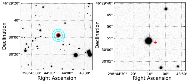
We kept Kepler-445 in focus during the observations. To ensure that Kepler-445 stayed on the same group of pixels, we did not dither in between exposures. With the exposure times listed in Table 1, the central pixel of Kepler-445’s point spread function typically registered 3 counts, which was well below the nonlinear response regime of the detector. Figure 1 shows a portion of a background-subtracted, raw Sloan z’-band image centered on Kepler-445.
The LMI has an e2v CCD231 detector, which is a 6144x6160-pixel deep depletion CCD. The readout time for the entire chip with 1x1 binning on a single amplifier is 73 seconds. Since our exposure times were always less than or equal to 30 seconds, we chose to increase efficiency by reading the chip with all four amplifiers and 2x2 binning. This decreased the overhead time in between exposures to 8.5 seconds. The effective pixel scale was 024 pixel-1 with 2x2 binning.
3. Data Analysis
3.1. Calibration
We employed a custom data reduction and analysis pipeline that has previously been applied to high-precision, time-series photometry from the DCT-LMI (Dalba & Muirhead, 2016). The calibration consisted of a bias and over scan subtraction and a flat-field correction. The minimal dark current present in the observations (estimated to be 0.07 electrons pixel-1 hour-1) was removed through the background subtraction described below.
In some cases, we applied an additional correction for fringing. Although the LMI’s deep depletion CCD suppressed fringing at long wavelengths, the Sloan z’-band images still displayed low-level fringe patterns with typical variability of less than 1%. The patterns were large and were difficult to detect in small portions of the full image (Fig. 1). We removed the fringing using a fringe frame constructed previously under a separate DCT program (P.I. E. Blanton). The fringe frame was created by median combining 17, 600-second Sloan z’-band images taken on UT 2013 November 02 and UT 2013 November 04. Each image was dithered by at least 15 to assure that sources fell on different pixels and would not appear in the final fringe frame. Each image also received a bias, over scan, and flat-field correction before being combined to create the fringe frame.
We scaled the fringe frame to each Kepler-445 science frame following the method of Snodgrass & Carry (2013) and using 45 “control pairs” to account for potential contamination by background sources. The scaled fringe frame was then subtracted from the science frame to remove the fringing.
3.2. Differential Aperture Photometry
We conducted differential aperture photometry on Kepler-445 using background stars in the 123x123 field-of-view of the DCT-LMI. The field was crowded, so we selected calibration stars based on the following criteria. First, the outer edge of sky annulus of the star could not be within 100 pixels of the edge of the frame. Second, the star’s sky annulus could not overlap the photometric aperture of any other source in the image. Third, the star’s count value could not enter the nonlinear response regime of the detector (4 counts) at any point throughout the observation. Fourth, the calibrator could not be a known variable star. Lastly, the star’s photometric aperture could not contain a cosmetic defect (e.g., dead pixels). These criteria yielded hundreds of potential calibration stars. We conducted photometry on each of these stars throughout the observations, although we did not use each star in the calculation of Kepler-445’s final light curve.
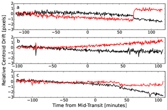
For each image, we first determined the centroids of Kepler-445 and all calibration stars by fitting a 2D Gaussian profile to the stellar point spread functions. The x- and y-centroid drifts of Kepler-445 are shown in Fig. 2. In most cases, the centroid stayed within a pixel or two of its original position.
We masked each bright source in the image to estimate the median global background value, which was subtracted from the entire image. We summed the flux from Kepler-445 and the calibration stars in the photometric apertures and used the sky annuli to account for any residual local background signal, including any dark current. In the sky annuli, bad pixels, hot pixels, cosmic ray strikes, and any other spurious signals at a level of 5 above or below the median count value were masked. We employed this two-stage background subtraction in order to monitor changes in local background across the quadrants of the detector that were read out by different amplifiers. At the time of the Kepler-445 observations, the multi-amplifier readout feature of the DCT-LMI had not been widely used. We did not measure local variations in background signal for any of the observations. Since the sky annuli were sufficiently large, the mean local background signals were approximately zero and the second subtraction had no effect on the resultant photometry.
The radii of the photometric apertures and sky annuli are provided in Table 1. These apertures yielded the lowest out-of-transit scatter in the final light curves of Kepler-445. Other aperture radii in the range [7,14] pixels—incremented by 0.5 pixels—returned less precise photometry.
Of the many potential calibration stars in the DCT-LMI field-of-view, only a subset was used to create a master calibration light curve. The subset was determined through the following procedure. First, each star’s light curve was normalized to the median count value of the exposures gathered before or after the transit of Kepler-445c. Then, for each of the stars, we defined a quality factor as
| (1) |
where was the number of exposures taken outside of Kepler-445c’s transit, was the median-normalized flux of Kepler-445 in the th exposure, and was the median-normalized flux of the th star in the th exposure. This factor described the out-of-transit deviation of each calibration star’s photometry from that of Kepler-445. We only continued analysis with the 15 calibration stars having the lowest -values. These 15 stars were distributed into 32767 unique sets. We calculated a master calibration light curve by taking the mean of all the light curves in each set. We normalized the flux of Kepler-445 to each of these 32767 master light curves, and only continued analysis on the one curve that yielded the lowest out-of-transit scatter. The calibration stars used to create final light curves of Kepler-445 for each observation are listed in Table 2. Each star was similar in brightness to Kepler-445, within 1.5 magnitudes in Sloan i’-band.
| KIC IDaaKepler Input Catalog (KIC, Brown et al., 2011) | Sloan i’-band | Observation Date |
|---|---|---|
| MagnitudebbMagnitudes from http://vizier.u-strasbg.fr/ | [UT] | |
| 9789729 | 14.541 | 2015/06/19 |
| 9790033 | 14.860 | 2015/06/19 |
| 9789938 | 14.913 | 2015/06/19 |
| 9789731 | 14.942 | 2015/06/19 |
| 9789958 | 14.718 | 2015/07/23 |
| 9790304 | 14.557 | 2015/07/23 |
| 9730187 | 15.493 | 2015/07/23 |
| 9730361 | 15.382 | 2015/07/23 |
| 9789836 | 15.335 | 2015/07/28 |
| 9729892 | 15.733 | 2015/07/28 |
| 9729667 | 15.355 | 2015/07/28 |
| 9790345 | 15.244 | 2015/07/28 |
| 9729595 | 16.540 | 2015/07/28 |
Note. — The Sloan i’-band magnitude of Kepler-445 is 16.0240.011 (Muirhead et al., 2015).
The master calibration light curves and the photometry of Kepler-445 prior to calibration are shown in Fig. 3. The flux from Kepler-445 and the calibration stars increased or decreased as the field rose or set. This variation was greatest for the first observation which sampled the widest range of airmass. The small, rapid variations were due to minor changes in transparency and other noise sources. The transits were visible as deviations between the Kepler-445 and calibration light curves. The photometry did not appear to exhibit systematic errors that could influence the values of transit depth derived later.

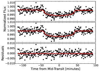
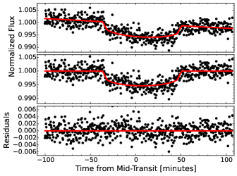
The final transit light curves for UT 2015 June 19, UT 2015 July 23, and UT 2015 July 28 are shown in Figs. 4, 5, and 6, respectively. The three observations displayed near-Gaussian scatter with 1 uncertainties of 0.26%, 0.23%, and 0.17%. The repeatable, high-precision photometry demonstrates that the DCT-LMI is a useful tool for transit photometry.
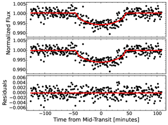
To date, only a few campaigns have utilized the DCT-LMI for high-precision transit photometry (e.g., Biddle et al., 2014; Dalba & Muirhead, 2016), so any time-correlated (red) noise present in this type of observation has not been fully characterized. To evaluate the extent of red noise in the Kepler-445 photometry, we employed the “time-averaging” method propounded by Pont et al. (2006) and used in numerous transit photometry studies (e.g., Winn et al., 2008). On the timescale of ingress (5–10 minutes), the binned residuals for each observation stayed very near to the expectation for Gaussian noise (Fig. 7). This suggested that our results were not greatly influenced by time-correlated uncertainty.
We also searched for correlation between the final photometry and the x- and y-centroid positions of Kepler-445 on the detector (Fig. 2). Once the background trend was removed from the photometry (§3.3), the Pearson correlation coefficients () between the out-of-transit flux and the centroids for each observation were small (), suggesting that there was no significant linear correlation.

3.3. Parameter Estimation
We fit the final light curves of Kepler-445 with transit models in order to determine the transit parameters for Kepler-445c. The purpose of this parameter estimation was not to fully recharacterize Kepler-445c or the Kepler-445 system, which we leave to future work (A. Mann et al. 2017, in preparation). Instead, we focused on the magnitude of Kepler-445c’s transit depth. As we demonstrate in §4, our ground-based observations differed significantly from those obtained with Kepler data as reported by Muirhead et al. (2015).
We employed the analytic transit models of Mandel & Agol (2002) in our fits to the DCT-LMI data. The transit parameters used by these models are described in Table 3. Following Kipping (2013), we included physically realistic quadratic limb darkening in the transit model with the parameters and as substitutes for and via the relations
| (2) |
We also fit for the slight background trend that existed in each observation (see the top panels of Figs. 4, 5, and 6). Although it was possible that this minor effect was astrophysical in nature (i.e., stellar variability), it was more likely a result of the changing airmass during the observations (Table 1) and other systematic errors. Regardless of its origin, we included in the fit a background signal () of the form
| (3) |
where was the time elapsed since the beginning of the observation and and were free parameters.
Following Muirhead et al. (2015), we held the orbital eccentricity () at zero during the model fitting under the assumption that the timescale for Kepler-445c to circularize was significantly less than the age of the Kepler-445 system. We also adopted the orbital period of Kepler-445c from Muirhead et al. (2015) in our fitting procedure since this was well constrained by the Kepler light curves and not influenced by the post-processing aperture contamination we describe later.
We used the Markov Chain Monte Carlo (MCMC) ensemble sampler emcee (Foreman-Mackey et al., 2013) to estimate the other transit parameters within a Bayesian framework and applied the uniform priors listed in Table 3. Since time-correlated noise was insignificant in these observations (§3.2), the uncertainties on each data point were defined to be the standard deviation of the out-of-transit flux. Furthermore, in evaluating the posterior distributions, the likelihood functions were assumed to be Gaussian. Each MCMC routine sampled the parameter space 2 times, and the chains converged on the best-fit value of each parameter within the first 30% of the total number of steps.
The best-fit parameters for each observation fitted individually are presented in Table 4. The scaled semi-major axis values (), which should not vary as a function of wavelength or time, agreed to within 1 across the observations. The limb darkening parameters were not well constrained but marginalizing over these uncertainties still yielded errors less than four percent on the best-fit planet-star radius ratios ().
The values of for the two Sloan i’ band observations (UT 2015 June 19 and UT 2015 July 28) were inconsistent to 2.1. The limb darkening parameters found for each of these Sloan i’ band observations also displayed notable differences. This may have resulted from the reduction in post-transit baseline observation suffered by the first Sloan i’-band observation. This loss of baseline increased the uncertainty in the estimation of the background trend, potentially allowing the background to artificially influence the transit parameters. The slight difference in observing conditions between the two Sloan i’-band nights may have also exacerbated the issue. The second Sloan i’-band transit, having a full out-of-transit baseline and the highest precision of any observation, was likely the more reliable measurement, and the differences in transit parameters mentioned here were likely not astrophysical in nature.
We extracted the best-fit transit parameters a second time by fitting all three observations simultaneously. The model used in this case had two global parameters ( and orbital inclination ), three filter-dependent parameters (, , and ), and three other local parameters (mid-transit time , , and ). The best-fit values of all jointly-fit parameters are listed in Table 5. As expected, the new value of was consistent with each individual observation. In this joint fit, the values of between Sloan i’ and Sloan z’ bands were consistent to within 1. As expected, the Sloan i’-band parameters favored the values from the UT 2015 July 28 observation, which were likely more reliable than those from UT 2015 June 19.
| Parameter | Value or Prior | Description |
|---|---|---|
| 0 | Orbital eccentricity. Fixed, from Muirhead et al. (2015) | |
| [days] | 4.871229 0.000011 | Orbital period. Fixed, from Muirhead et al. (2015) |
| [20.41,34.01] | Semi-major axis scaled to stellar radius | |
| [degrees] | [88.9,90] | Orbital inclination |
| - 2457192 [JD] | [0.75,0.79] | Time of mid-transit on UT 2015 June 19 |
| - 2457226 [JD] | [0.85,0.90] | Time of mid-transit on UT 2015 July 23 |
| - 2457231 [JD] | [0.73,0.79] | Time of mid-transit on UT 2015 July 28 |
| [0,1] | Limb darkening parameter 1 (Kipping, 2013) | |
| [0,1] | Limb darkening parameter 2 (Kipping, 2013) | |
| [0.001,0.01] | Planet-star radius ratio | |
| [-0.01,0.01] | 0th order background parameter (Eq. 3) | |
| [days-1] | [-0.05,0.05] | 1st order background parameter (Eq. 3) |
Note. — [,] signifies a uniform prior probability distribution in the range [,].
| Parameter | UT 2015 June 19 | UT 2015 July 23 | UT 2015 July 28 |
|---|---|---|---|
| 26.0 | 26.2 | 25.7 | |
| [degrees] | 89.50 | 89.49 | 89.51 |
| - 2457100 [JD] | 92.76836 | 126.88548 | 131.75565 |
| 0.55 | 0.43 | 0.66 | |
| 0.46 | 0.51 | 0.74 | |
| 0.64 | 0.63 | 1.13 | |
| 0.06 | -0.02 | -0.37 | |
| 0.0727 | 0.0662 | 0.0651 | |
| 0.00139 | 0.00168 | 0.00047 | |
| [days-1] | -0.0045 | -0.0280 | -0.0004 |
Note. — The upper and lower uncertainties of each parameter were calculated using the 16th, 50th, and 84th percentiles of the posterior distributions. See Table 3 for descriptions of the parameters and priors.
| Parameter | Value |
|---|---|
| Global | |
| 26.2 | |
| [degrees] | 89.54 |
| Sloan i’ | |
| 0.0675 | |
| 0.55 | |
| 0.68 | |
| 0.99 | |
| -0.27 | |
| Sloan z’ | |
| 0.0657 | |
| 0.50 | |
| 0.48 | |
| 0.65 | |
| 0.03 | |
| UT 2015-06-19 | |
| - 2457100 [JD] | 92.76818 |
| 0.00122 | |
| [days-1] | -0.0059 |
| UT 2015-07-23 | |
| - 2457100 [JD] | 126.88555 |
| 0.00168 | |
| [days-1] | -0.0280 |
| UT 2015-07-28 | |
| - 2457100 [JD] | 131.75562 |
| 0.00055 | |
| [days-1] | -0.0004 |
Note. — The upper and lower uncertainties of each fitted parameter were calculated using the 16th, 50th, and 84th percentiles of the posterior distributions. See Table 3 for descriptions of the parameters and priors.
4. Results
4.1. The Revised Transit Depth of Kepler-445c
We estimated the transit depths of Kepler-445c in the Sloan i’ and z’ bands using the best-fit parameters in Table 5. For each filter, we created 1000 theoretical light curves by drawing samples from the posterior distributions of the transit parameters. From these light curves, we determined the posterior distribution of transit depths. In the Sloan i’ and z’ bands, these depths were 0.6180.022% and 0.5450.028%, respectively. These values were consistent with each other to 2.1 confidence.
It was unlikely, although not impossible, that the difference between the transit depths was a result of Kepler-445c’s atmospheric properties. Most exoplanets similar to Kepler-445c (e.g., GJ 1214b, HD 97658b, GJ 436b, Kreidberg et al., 2014; Knutson et al., 2014a, b) have been found to host atmospheres with high-altitude clouds, hazes, or high mean molecular weights that produce flat transmission spectra. If this was true of Kepler-445c’s atmosphere as well, one would expect the Sloan i’- and z’-band transit depths to be consistent. The difference, then, could stem from a slight underestimation of the uncertainties on the transit parameters such that the posterior distribution of transit depths was artificially narrow. Regardless of the origin of the inconsistency, the transit depths estimated from the three DCT-LMI observations described here were likely not precise enough to distinguish between various atmospheric compositions for Kepler-445c.
Continuing under the assumption that the variation in transit depths between filters was not astrophysical in nature, we calculated a combined value of transit depth by taking the mean of the two values listed above: 0.5820.026%. The uncertainty was the standard error of the mean defined as where was the sample standard deviation and was the number of samples, which in this case was two.
4.2. The Previous Transit Depth of Kepler-445c
The Kepler-445 system was first characterized with long-cadence Kepler PDCSAP data by Muirhead et al. (2015). The and values for Kepler-445c reported by that work are 30.21 0.38 and 0.1075 0.0014, which are also the values currently listed on the NASA Exoplanet Archive.222 http://exoplanetarchive.ipac.caltech.edu/ These values disagree with the and estimated from the DCT observations to 3.2 and greater than 17, respectively.
Additionally, visual inspection of the phase-folded light curves of Muirhead et al. (2015, Figure 5) suggests that the transit depth is at least one percent. Muirhead et al. (2015) does not explicitly report a transit depth, although exoplanets.org currently cites that work for a depth of 1.16%, more than twice the value reported here.333Database accessed on 2016 November 21. Differences in limb darkening can alter transit depths obtained through different filters (e.g., Knutson et al., 2007), however, this discrepancy seems too large to be attributed entirely to limb darkening.
Since the Kepler-445 system was first characterized, new observations of Kepler-445 may result in updated stellar parameters (A. Mann et al. 2017, in preparation). These new parameters may alter the physical characteristics of Kepler-445c, but would not explain the differences in transit depth between the Kepler and DCT-LMI transit curves.
4.3. The Crowding Metric in the Kepler Pipeline
The discrepancy between the transit depths of Kepler-445c is a result of the crowding metric applied by the pre-search data conditioning (PDC) module of the Kepler pipeline (Stumpe et al., 2012; Smith et al., 2012). This metric, defined as “CROWDSAP” in the header of the Kepler light curve files, is the ratio of the target flux to the total flux in the photometric aperture. It is a quarterly-averaged, scalar value between zero and unity. Only the PDCSAP version of the flux reported by Kepler is adjusted by this crowding factor.
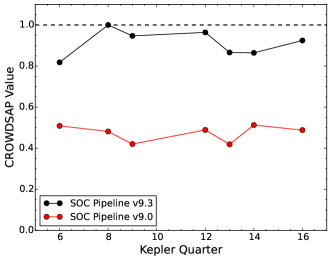
The value of CROWDSAP for a given star may vary from quarter to quarter as it falls on different regions of the detector and is processed with different pixel response functions (PRFs) and optimal photometric apertures. The value of CROWDSAP reported in the Kepler data also depends on the version of the Science Operations Center (SOC) pipeline that processed the data. In Fig. 8, we show the CROWDSAP values for Kepler-445 data processed with versions 9.0 and 9.3 of the SOC pipeline. Between version 9.0, which processed the data used by Muirhead et al. (2015), and version 9.3, which was released in December 2015,444See the Kepler Data Release Notes 25 available on the Barbara A. Mikulski Archive for Space Telescopes (MAST). the mean value of CROWDSAP changed from 0.470.04 to 0.910.06, a 6.1 increase.
CROWDSAP values can be directly affected by changes to the optimal photometric apertures, which occasionally change when the Kepler pipeline is updated. After an update, the pipeline may determine that a different photometric aperture increases the combined differential photometric precision (CDPP, Christiansen et al., 2012) in the resultant light curve of a particular star. If this new aperture now contains flux from nearby sources, then the CROWDSAP parameter should change accordingly.
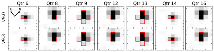
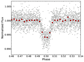
As demonstrated by Fig. 9, the optimal photometric apertures for Kepler-445 were largely unchanged between versions 9.0 and 9.3 of the pipeline. With the exception of minor changes in Quarters 12 and 16, the apertures covered the same groups of pixels and yet the CROWDSAP values increased dramatically. From an increase in the average value of the crowding metric, we would expect a corresponding decrease in transit depth. Inspection of the Kepler-445c transit curves produced by version 9.3 of the SOC pipeline confirmed this expectation. In Fig. 10, we show the phase-folded PDCSAP photometry of Kepler-445 from all quarters of observation. The photometry was flattened using the kepflatten task in PyKE555https://keplerscience.arc.nasa.gov/software.html (Still & Barclay, 2012) and phase-folded according to the ephemeris in Muirhead et al. (2015) for Kepler-445c. Visual inspection of the phase-folded photometry suggested a transit depth of 0.6%, which was consistent with the DCT-LMI light curves.
The ratio between the DCT-LMI transit depth of Kepler-445c (0.5820.026%) and the previously published transit depth666See exoplanets.org, which cites Muirhead et al. (2015). (1.160.28%) equals 0.500.12. This value agrees with the ratio of mean CROWDSAP values between versions 9.0 and 9.3 of the SOC pipeline, 0.520.06, to well within 1. Therefore, the change in the crowding metric offers a highly consistent explanation for the discrepant Kepler-445c transit depths discovered by this work.
The 6.1 increase in mean CROWDSAP value for Kepler-445 between the two aforementioned versions of the SOC pipeline results from a new method of constructing the stellar “scene,” which contains all stars besides the target and any zodiacal light (Bryson et al., 2010). Before version 9.3 of the SOC pipeline, the scene was determined with the predicted PRF model and the stellar data in the KIC. In version 9.3, however, stellar scenes are reconstructed through a photometric analysis of the actual pixel level data (Twicken et al., 2016). This new method maximizes the CDPP in the photometric aperture and removes an inherent susceptibility to stellar position and magnitude errors that may be present in the KIC. The optimal photometric apertures may change in response to the new stellar scenes and influence the crowding metrics. However, in the case of Kepler-445, the CROWDSAP variations were not caused by changes in photometric apertures.
4.4. A Phantom Star in the Scene of Kepler-445
The SOC pipeline update and subsequent change in CROWDSAP values identified an unusual circumstance surrounding the characterization of exoplanet Kepler-445c. According to the KIC, another source known as KIC 9730159 existed away from Kepler-445. The object class of KIC 9730159 was reported as “star” and the condition flag was empty (i.e., KIC 9730159 was not flagged as an artifact, planetary-candidate, or exoplanet). KIC 9730159 had a Kepler magnitude of 17.667, which was 1.1% greater than that of Kepler-445. Given the plate scale of our DCT-LMI observations (024 pixel-1), we would have expected KIC 9730159 to be present in the images 9 pixels away from Kepler-445, well outside the full width at half maximum of the point spread function even during the worst seeing we experienced. Yet KIC 9730159 was not present in the DCT-LMI images (Fig. 1). KIC 9730159 was also not visible in the J-band United Kingdom Infrared Telescope (UKIRT)777Database release “ukidssdr10plus,” http://wsa.roe.ac.uk/ images of the Kepler field (Fig. 1). Muirhead et al. (2015) reported a non-detection of KIC 9730159, postulating that the KIC may have accidentally registered Kepler-445 twice.
We explored the hypothesis that KIC 9730159 was a phantom star—present in the KIC and the data conditioning, but not an actual star—in more detail. KIC 9730159 originated in the USNO-B catalog where its designation was 1364-0336533 and its mean epoch of observation was 1990.2. It had a high proper motion (RA: mas, DEC: mas) and a correspondingly large uncertainty in its J2000 coordinates. Monet et al. (2003) warned that objects with large proper motions may be erroneously assigned in future observations and may lead to catalog entries for blank patches of sky. This is a highly probable explanation for the existence of KIC 9730159. Kepler-445 (USNO-B1 designation 1364-0336538) also had a relatively high proper motion, but its mean epoch of observation was 1977.1. KIC 9730159 was likely “created” as a result of an observation of Kepler-445 circa 1990 that was mistakenly assigned to a new star. Furthermore, the USNO-B1 catalog reported three detections of this phantom star, allowing it to pass the threshold for acceptance into the KIC (Brown et al., 2011).
Together, the USNO-B phantom star inherited by the KIC, the original method used to construct the stellar scene of Kepler-445, and the timing of the initial characterization of Kepler-445c formed an improbable series of events that led to the overestimation of the transit depth of Kepler-445c.
5. Discussion
5.1. Are All the Planets in the Kepler-445 System Rocky?
The original radius of Kepler-445c, 2.510.36 (Muirhead et al., 2015), placed it in the interesting regime of exoplanets with sizes between the Earth and Neptune that are highly amenable to atmospheric characterization (e.g., Fraine et al., 2014; Kreidberg et al., 2014; Knutson et al., 2014a, b). With ground-based observations of additional transits of this exoplanet, we found that the transit depth and planetary radius were overestimated. Using the value of obtained from the joint fit to all the DCT Sloan i’-band observations888We choose the value from Sloan i’ band over Sloan z’ band based on the parameter uncertainties. and employing the Kepler-445 stellar radius from Muirhead et al. (2015), we find the revised radius of Kepler-445c to be 1.550.23.
In addition to Kepler-445c, this system contains two smaller exoplanets: Kepler-445b and Kepler-445d. As reported in Muirhead et al. (2015), the b and d planets have radii of 1.580.23 and 1.250.19, respectively. Although we did not acquire transit observations of these exoplanets, their Kepler light curves were subject to the same analysis and crowding contamination as that of Kepler-445c. Here, we scale their Kepler transit depths using the ratio of CROWDSAP values before and after the SOC pipeline update (§4.3) and briefly discuss the potential nature of these small exoplanets.
The previously measured transit depths of Kepler-445b and Kepler-445d are 0.460.36% and 0.280.58%, respectively.999See exoplanets.org, which cites Muirhead et al. (2015). Multiplying these depths by a factor of 0.52 to correct for the phantom star aperture contamination yields depths of 0.24% and 0.15%. Estimating the transit depth as and applying the Kepler-445 stellar radius from Muirhead et al. (2015) yields planetary radii of and . The large uncertainties on the transit depths, however, prevent precise estimation of the planetary radii.
As an alternative means of estimating the planetary radii, we scaled the values for Kepler-445b and Kepler-445d to reflect the change in this parameter for Kepler-445c discovered by this work. Again employing the Kepler-445 stellar radius from Muirhead et al. (2015), we estimate planetary radii of 0.980.14 and 0.770.12 for Kepler-445b and Kepler-445d, respectively.
Despite their Earth-like size, none of the exoplanets in the Kepler-445 system orbit within the habitable zone (Muirhead et al., 2015), meaning that none of them are Earth-analogs. It is interesting that the revised radii of all three planets are at or below the threshold of 1.6 from Rogers (2015), suggesting that all three have primarily rocky compositions. Perhaps, the potentially rocky compositions of short-period exoplanets in systems such as Kepler-42 (e.g., Muirhead et al., 2012), Kepler-446 (Muirhead et al., 2015), TRAPPIST-1 (Gillon et al., 2016), and K2-72 (e.g., Crossfield et al., 2016; Vanderburg et al., 2016) in addition to Kepler-445b, c, and d imply that the formation of small, rocky planets around M-dwarfs is an efficient process.
However, as is true in all studies of transiting exoplanets, the validity of these conclusions is predicated upon the accuracy of the characterization of the host star, Kepler-445. All radii mentioned here rely on the current stellar model (Muirhead et al., 2015), and may change upon further characterization (A. Mann et al. 2017, in preparation).
5.2. The Potential for Additional Phantom Stars in the KIC
Every star known (or thought) to exist in the Kepler field-of-view was assigned a KIC identifier and a Kepler magnitude. As a result, sources from many catalogs with various levels of accuracy were incorporated into the KIC. Although each source underwent a thorough vetting procedure (Brown et al., 2011), there were bound to be spurious additions, such as KIC 9730159. Since the original characterization of Kepler-445c, the updates to the SOC pipeline have increased the accuracy of the CROWDSAP values for all KIC sources. These updates corrected the transit depth of Kepler-445c and greatly reduced the probability of errors in the KIC contaminating other Kepler PDCSAP light curves.
However, it is possible that other phantom stars exist in the KIC and influence the photometry of other Kepler targets. The authors contributed a discussion on this topic to the 2016 August 8 version of the Kepler Data Release Notes 25 on MAST.101010Section A.1.2, https://archive.stsci.edu/kepler/data_release.html Conducting a direct search for phantom stars is a challenging task given the number of sources comprising the KIC. Indirect searches (e.g., by flux or transit depth changes between different pipeline versions) are also complicated since large CROWDSAP variations can correctly accompany changes in the optimal photometric apertures. Furthermore, different versions of the pipeline typically operate with different amounts of data. The sensitivity added by additional transits must also be considered when searching for phantom stars indirectly.
Phantom stars are likely a rare occurrence. However, their presence could cause systematic shifts in stellar crowding between pipeline versions and could alter transit depths and inferred planetary radii. This has the potential to affect investigations that make use of the PDCSAP transit depths for a large number of exoplanets, where individual follow-up observation of each is not possible (e.g., studies of planet occurrence rates, planet populations, or transit signal recovery efficiencies).
The sizes of exoplanets in the perplexing Earth-to-Neptune regime only span a few Earth radii. A factor of two correction to the transit depth, corresponding to a change in planetary radius, can therefore crucially alter the interpretation of a planet’s interior and atmosphere. In this way, assessing the crowding in the scene of an exoplanet host—which is a necessary step in the data conditioning process—has the potential to obscure the understanding of these exoplanets further. Although the case of Kepler-445c was highly improbable, it emphasizes the level of caution that must be exercised when analyzing and interpreting data from exoplanet transit surveys.
5.3. Implications for TESS
In the near future, the Transiting Exoplanet Survey Satellite (TESS) is expected to launch and begin surveying the entire sky for nearby exoplanets (Ricker et al., 2015). Whereas the pixels on the Kepler detectors have a plate scale of pixel-1, TESS’ pixels will cover even more sky, with pixel-1. TESS will therefore be even more susceptible to crowding and stellar catalog errors than Kepler. The analysis of TESS observations will of course be informed by the many lessons learned from the Kepler data set, and a careful treatment of the crowding metric should be no exception.
References
- Biddle et al. (2014) Biddle, L. I., Pearson, K. A., Crossfield, I. J. M., et al. 2014, MNRAS, 443, 1810
- Borucki et al. (2010) Borucki, W. J., Koch, D., Basri, G., et al. 2010, Sci, 327, 977
- Brown et al. (2011) Brown, T. M., Latham, D. W., Everett, M. E., & Esquerdo, G. A. 2011, AJ, 142, 112
- Bryson et al. (2010) Bryson, S. T., Tenenbaum, P., Jenkins, J. M., et al. 2010, ApJ, 713, L97
- Burke et al. (2014) Burke, C. J., Bryson, S. T., Mullally, F., et al. 2014, ApJS, 210, 19
- Cartier et al. (2015) Cartier, K. M. S., Gilliland, R. L., Wright, J. T., & Ciardi, D. R. 2015, ApJ, 804, 97
- Cassan et al. (2012) Cassan, A., Kubas, D., Beaulieu, J.-P., et al. 2012, Natur, 481, 167
- Christiansen et al. (2012) Christiansen, J. L., Jenkins, J. M., Caldwell, D. A., et al. 2012, PASP, 124, 1279
- Crossfield et al. (2016) Crossfield, I. J. M., Ciardi, D. R., Petigura, E. A., et al. 2016, ApJS, 226, 7
- Dalba & Muirhead (2016) Dalba, P. A., & Muirhead, P. S. 2016, ApJ, 826, L7
- Foreman-Mackey et al. (2013) Foreman-Mackey, D., Hogg, D. W., Lang, D., & Goodman, J. 2013, PASP, 125, 306
- Fraine et al. (2014) Fraine, J., Deming, D., Benneke, B., et al. 2014, Natur, 513, 526
- Fressin et al. (2013) Fressin, F., Torres, G., Charbonneau, D., et al. 2013, ApJ, 766, 81
- Gillon et al. (2016) Gillon, M., Jehin, E., Lederer, S. M., et al. 2016, Natur, 533, 221
- Jenkins et al. (2010) Jenkins, J. M., Caldwell, D. A., Chandrasekaran, H., et al. 2010, ApJ, 713, L87
- Kinemuchi et al. (2012) Kinemuchi, K., Barclay, T., Fanelli, M., et al. 2012, PASP, 124, 963
- Kipping (2013) Kipping, D. M. 2013, MNRAS, 435, 2152
- Knutson et al. (2014a) Knutson, H. A., Benneke, B., Deming, D., & Homeier, D. 2014a, Natur, 505, 66
- Knutson et al. (2007) Knutson, H. A., Charbonneau, D., Noyes, R. W., Brown, T. M., & Gilliland, R. L. 2007, ApJ, 655, 564
- Knutson et al. (2014b) Knutson, H. A., Dragomir, D., Kreidberg, L., et al. 2014b, ApJ, 794, 155
- Koch et al. (2010) Koch, D. G., Borucki, W. J., Basri, G., et al. 2010, ApJ, 713, L79
- Kreidberg et al. (2014) Kreidberg, L., Bean, J. L., Désert, J.-M., et al. 2014, Natur, 505, 69
- Mandel & Agol (2002) Mandel, K., & Agol, E. 2002, ApJ, 580, L171
- Massey et al. (2013) Massey, P., Dunham, E. W., Bida, T. A., et al. 2013, in American Astronomical Society Meeting Abstracts, Vol. 221, 2013AAS 221, 345.02
- Monet et al. (2003) Monet, D. G., Levine, S. E., Canzian, B., et al. 2003, AJ, 125, 984
- Morton (2012) Morton, T. D. 2012, ApJ, 761, 6
- Muirhead et al. (2012) Muirhead, P. S., Johnson, J. A., Apps, K., et al. 2012, ApJ, 747, 144
- Muirhead et al. (2015) Muirhead, P. S., Mann, A. W., Vanderburg, A., et al. 2015, ApJ, 801, 18
- Mullally et al. (2016) Mullally, F., Coughlin, J. L., Thompson, S. E., et al. 2016, PASP, 128, 074502
- Petigura et al. (2013) Petigura, E. A., Howard, A. W., & Marcy, G. W. 2013, PNAS, 110, 19273
- Pont et al. (2006) Pont, F., Zucker, S., & Queloz, D. 2006, MNRAS, 373, 231
- Quintana et al. (2010) Quintana, E. V., Jenkins, J. M., Clarke, B. D., et al. 2010, in Proc. SPIE, Vol. 7740, Software and Cyberinfrastructure for Astronomy, 77401X
- Ricker et al. (2015) Ricker, G. R., Winn, J. N., Vanderspek, R., et al. 2015, JATIS, 1, 014003
- Rogers (2015) Rogers, L. A. 2015, ApJ, 801, 41
- Rowe et al. (2014) Rowe, J. F., Bryson, S. T., Marcy, G. W., et al. 2014, ApJ, 784, 45
- Smith et al. (2012) Smith, J. C., Stumpe, M. C., Van Cleve, J. E., et al. 2012, PASP, 124, 1000
- Snodgrass & Carry (2013) Snodgrass, C., & Carry, B. 2013, Msngr, 152, 14
- Still & Barclay (2012) Still, M., & Barclay, T. 2012, PyKE: Reduction and analysis of Kepler Simple Aperture Photometry data, Astrophysics Source Code Library, ascl:1208.004
- Stumpe et al. (2012) Stumpe, M. C., Smith, J. C., Van Cleve, J. E., et al. 2012, PASP, 124, 985
- Torres et al. (2011) Torres, G., Fressin, F., Batalha, N. M., et al. 2011, ApJ, 727, 24
- Tsiaras et al. (2016) Tsiaras, A., Rocchetto, M., Waldmann, I. P., et al. 2016, ApJ, 820, 99
- Twicken et al. (2010) Twicken, J. D., Clarke, B. D., Bryson, S. T., et al. 2010, in Proc. SPIE, Vol. 7740, Software and Cyberinfrastructure for Astronomy, 774023
- Twicken et al. (2016) Twicken, J. D., Jenkins, J. M., Seader, S. E., et al. 2016, AJ, 152, 158
- Vanderburg et al. (2016) Vanderburg, A., Latham, D. W., Buchhave, L. A., et al. 2016, ApJS, 222, 14
- Winn et al. (2008) Winn, J. N., Holman, M. J., Torres, G., et al. 2008, ApJ, 683, 1076
- Ziegler et al. (2016) Ziegler, C., Law, N. M., Morton, T., et al. 2016, arXiv:1605.03584, AJ in press