Accretion and Magnetic Reconnection in the Classical T Tauri Binary DQ Tau

Abstract

Binary star-formation theory predicts that close binaries ($a<100$ AU) will experience periodic pulsed accretion events as streams of material form at the inner edge of a circumbinary disk, cross a dynamically cleared gap, and feed circumstellar disks or accrete directly onto the stars. The archetype for the pulsed-accretion theory is the eccentric, short-period, classical T Tauri binary DQ Tau. Low-cadence ($\sim$daily) broadband photometry has shown brightening events near most periastron passages, just as numerical simulations would predict for an eccentric binary. Magnetic reconnection events (flares) during the collision of stellar magnetospheres near periastron could, however, produce the same periodic, broadband behavior when observed at a one-day cadence. To reveal the dominate physical mechanism seen in DQ Tau’s low-cadence observations, we have obtained continuous, moderate-cadence, multi-band photometry over 10 orbital periods, supplemented with 27 nights of minute-cadence photometry centered on 4 separate periastron passages. While both accretion and stellar flares are present, the dominant timescale and morphology of brightening events are characteristic of accretion. On average, the mass accretion rate increases by a factor of 5 near periastron, in good agreement with recent models. Large variability is observed in the morphology and amplitude of accretion events from orbit-to-orbit. We argue this is due to the absence of stable circumstellar disks around each star, compounded by inhomogeneities at the inner edge of the circumbinary disk and within the accretion streams themselves. Quasi-periodic apastron accretion events are also observed, which are not predicted by binary accretion theory.

1. INTRODUCTION

One of the primary outcomes of binary star formation theory is that the interaction between close binary star systems and their disk(s) is fundamentally different than the well-established single-star paradigm. In single stars, interplay between the star and disk is mediated by the stellar magnetic field (Shu et al., 1994; Hartmann et al., 1994). In this magnetic accretion model, strong stellar magnetic fields truncate the inner edge of the disk at the distance where viscous ram pressure balances the magnetic pressure. This “magnetospheric radius” is modeled as 5–10 stellar radii ($\sim$0.05AU; Johnstone et al. 2014) for typical pre-MS magnetic field strengths ($\sim$1–2 kG; Johns-Krull 2007) and accretion rates (10^-12–$10^{-8}M_{\odot}$ yr^-1; Alcalá et al. 2014). Inside this radius, material is confined to flow along magnetic field lines where it impacts the stellar surface at magnetic footpoints, shock-heating the photosphere (Orlando et al., 2013).

The single-star magnetic accretion model plays a critical role in the evolution of the star-disk system. For the star, it provides an avenue for continued mass growth while regulating the stellar angular momentum through magnetic disk locking (Shu et al., 1994). For the disk, accretion processes set the evolution timescale by controlling the consumption rate, outflow rates through wind and jet launching, and the intensity of UV radiation relevant for photoevaporation and disk chemistry (Alexander et al., 2014). By governing the stability, lifetime, and chemistry of protoplanetary disks, the star-disk interaction plays a vital role in the formation and evolution planets.

The successes of the single-star accretion paradigm and its impact on the evolution of the star-disk system highlights the need to characterize the binary-disk interaction. Most pressing is the indication that binary and higher multiple systems are a common outcome of star-formation (Raghavan et al., 2010). Kraus et al. (2011), for instance, find that up to 75% of Class II/III members of the Taurus-Auriga star-forming region are in multi-star systems. In binary systems with separations on the order of typical protostellar disk radii ($\sim$100s of AU; Jensen et al. 1996; Harris et al. 2012) the single-star model cannot simply be applied to environments where the distribution of disk material and mass flows are more complex. While theory describing binary-disk interaction is advancing, many of its predictions remain untested and therefore the effects of binarity on star and planet formation remains largely unconstrained.

Theory describing the binary-disk interaction in short-period systems has made two predictions that portray a complex and variable environment compared to single-stars. First, through co-rotational and Lindblad resonances, orbital motion will dynamically clear a central region around the binary creating up to three stable accretion disks: a circumstellar disk around each star and an encompassing circumbinary disk (Artymowicz & Lubow, 1994). Observational support for this spatial structure has come from modeling the IR spectral energy distribution (SED) of spectroscopic binaries (Jensen & Mathieu, 1997; Boden et al., 2009) and from spatially resolving central gaps from scattered light (Beck et al., 2012) and mm/sub-mm images (Andrews et al., 2011; Harris et al., 2012) of longer-period systems.

Table 1DQ Tau System Summary

Parameter	Value	Reference
P (days)	$15.80158\pm 0.00066$	1
$e$	$0.568\pm 0.013$	1
Tperi (HJD-2,400,000)	$47433.507\pm 0.094$	1
$a$ ($R_{\odot}$)	$28.96\pm 0.48$	1
$q\equiv$ M2/M1	$0.936\pm 0.051$	1
Periastron Separation ($R_{\odot}$)	$12.51\pm 0.43$	1
Apastron Separation ($R_{\odot}$)	$45.42\pm 0.43$	1
i (∘)	$158\pm 2$	1
Rotation Period (d)	$\sim$2	2
Disk $M_{\rm gas}$ ($10^{-4}M_{\odot}$)	$>$10	3
Disk $M_{\rm dust}$ ($10^{-4}M_{\odot}$)	0.90	3
d (pc)	140	4
$A_{V}$	$1.5\pm 0.3$	5
Primary
$M_{1}$ ($M_{\odot}$)	$0.63\pm 0.13$	1
$T_{1}$ ($K$)	$3700\pm 200$	1
$L_{1}$ ($L_{\odot}$)	$0.19\pm 0.07$	1
$R_{1}$ ($R_{\odot}$)	$1.05\pm 0.22$	1
Secondary
$M_{2}$ ($M_{\odot}$)	$0.59\pm 0.13$	1
$T_{2}$ ($K$)	$3500\pm 175$	1
$L_{2}$ ($L_{\odot}$)	$0.13\pm 0.07$	1
$R_{2}$ ($R_{\odot}$)	$1.00\pm 0.21$	1

Note. — ⁽¹⁾(Czekala et al., 2016), ⁽²⁾(Basri et al., 1997), ⁽³⁾(Williams & Best, 2014), ⁽⁴⁾(Kenyon et al., 1994), ⁽⁵⁾(This work)

Second, hydrodynamical models predict that circumbinary disk material will periodically form an accretion stream that crosses the cleared gap to feed circumstellar disks or accrete directly onto the stars themselves (Artymowicz & Lubow, 1996). Observations of ongoing accretion in pre-MS binary stars necessitates this refueling behavior to balance the short timescale on which a dynamically truncated circumstellar disk would be exhausted through viscous accretion.

Driven by binary orbital motion, predictions for the frequency of circumbinary accretion streams and their impact on stellar accretion rates are highly dependent on the binary orbital parameters (Günther & Kley, 2002; de Val-Borro et al., 2011; Gómez de Castro et al., 2013). Orbital eccentricity in particular has a large effect where, for a given mass ratio, the amplitude and “sharpness” of accretion events (in orbital phase) are predicted to increase with increasing eccentricity. Muñoz & Lai (2016, hereafter ML2016) for instance predict that equal-mass, circular binaries will experience long-duration (multiple orbital periods) accretion enhancements that occur every $\sim$5 orbital periods with a factor of 2 increase in the accretion rate at peak. A highly eccentric equal-mass binary, on the other hand, is predicted to exhibit sharp accretion events every orbit that evolve over roughly one-third of the orbital period and increase the accretion rate by more than a factor of 10 at peak. With these orbital parameter dependencies, short-period, eccentric systems provide the best opportunity to test accretion models.

Focusing on this advantageous corner of the eccentricity-period parameter space (analogous to DQ Tau; Table 1), the general consensus of models is that each apastron passage (orbital phase $\phi$=0.5) will induce a stream of material from the circumbinary disk (CBD) that feeds a burst of accretion during periastron passage ($\phi$=0,1). The specific morphology and amplitude of the accretion events varies from one modeling effort to the next (i.e. saw-toothed vs. symmetric rise and decay). Also, binary accretion simulations to date have yet to include a magnetohydrodynamic (MHD) treatment, which undoubtedly plays an important role close to the stars (e.g. Kulkarni & Romanova 2008). If these models are representative of binary accretion, they would imply very different angular momentum histories compared to single stars and a more dynamic disk environment relevant for planet formation.

1.1. DQ Tau

Since its discovery as a pre-main sequence (pre-MS) spectroscopic binary, DQ Tau has become one of the primary targets in confronting theory of the binary-disk interaction (Mathieu et al., 1997; Basri et al., 1997). Meeting the criteria of a classical T Tauri star (CTTS) with evidence of ongoing accretion and a gaseous protoplanetary disk, DQ Tau is one of a few, well-characterized pre-MS binary systems capable of informing the physics of star and planet formation in the binary environment.

The most extensive characterization of DQ Tau comes from Czekala et al. (2016). Their study combines the orbital solution from high-resolution, optical spectroscopy with disk kinematics derived from ALMA observations to jointly constrain the orbital parameters, stellar characteristics, and critically, the orbital inclination of the system. We compile their results and other relevant system parameters from other works in Table 1.

DQ Tau was the first source to provide observational evidence for the pulsed accretion theory. At many, but not all, periastron passages the system exhibited sharp increases in both broadband and H$\alpha$ luminosities (Mathieu et al., 1997; Basri et al., 1997), the same orbital phase predicted by simulations with DQ Tau’s orbital parameters (Artymowicz & Lubow, 1996). Broad and variable H$\alpha$ emission line profiles provided support that accretion was, at least in part, the source of the photometric variability. Subsequent studies in the NIR also supported the pulsed accretion interpretation with detections of diffuse, warm gas within a cleared central cavity (Carr et al., 2001; Boden et al., 2009). These results were limited however in their temporal and/or wavelength coverage. Sparse spectroscopic and interferometric observations provide valuable snap-shots of the system but are unable to test the temporal predictions of binary accretion theory. Even the Mathieu et al. (1997) $V$-band photometry ($\sim$10 observations per orbit) was only marginally sensitive to accretion, compared to $U$-band for instance (e.g. Venuti et al. 2014), and lacked the time-resolution necessary to test accretion models in detail.

While the above studies provide encouraging results for pulsed accretion theory, the quasi-periodic broadband, photometric behavior observed in DQ Tau is not exclusive to periodic enhanced accretion events alone. Magnetic reconnection events on low mass stars can create optical flares with the same general broadband characteristics of accretion. During magnetic reconnection, magnetic energy is converted into kinetic energy accelerating electrons along field lines. In stellar flares, these flows impact the chromosphere and photosphere where relativistic electrons deposit their energy creating a photospheric hot-spot and white-light excess very similar to that of accretion (e.g. compare Kowalski et al. 2013 and Herczeg & Hillenbrand 2008). Stellar flares are stochastic events but in a highly eccentric binary like DQ Tau, orbital motion brings the stars from $\sim$43 stellar radii ($R_{\star}$) at apastron to $\sim$12$R_{\star}$ at closest approach where the collision between each star’s magnetosphere may induce a series of magnetic reconnection events. Salter et al. (2010) find evidence for such events with observations of recurrent synchrotron, mm-wave flares (typical of stellar/solar flares) near the periastron passages of DQ Tau. If these events are capable of depositing their energy in the stellar surface, a large magnetic reconnection event or series of them could create optical flares near periastron that masquerade as the signal of periodic enhanced accretion in low-cadence broadband photometry. High-cadence, multi-color photometry, however, can distinguish between stellar flares and accretion variability.

In an effort determine the primary physical mechanism behind DQ Tau’s photometric variability, we have carried out an extensive monitoring campaign combining moderate and high-cadence optical photometry spanning more than 10 orbital periods. Our observations are capable of detecting and characterizing periodic pulsed accretion while determining the contribution from magnetic reconnection events. By monitoring the accretion rate as a function of orbital phase, these data provide a direct test of binary accretion theory and will extend our understanding of the star-disk interaction to binary systems.

A description of our observations is provided in Section 2 as well as our data reduction and calibration procedures. In Section 3 we discuss the morphology of our lightcurves and determine the dominant physical mechanism behind DQ Tau’s variability. We also characterize magnetic reconnection events and their frequency, and place our results in context of the colliding magnetosphere scenario. In Section 4 we calculate mass accretion rates, establish the presence of periodic enhanced accretion events, and comment on their variability. Section 5 provides a summary of our results.

2. OBSERVATIONS & DATA REDUCTION

Observations capable of detecting and characterizing pulsed accretion events in pre-MS binaries require multi-color photometric coverage over many orbital cycles at a cadence that is a fraction of the orbital period. These formidable demands are well met by the capabilities of the Las Cumbres Observatories Global Telescope (LCOGT) Network (Brown et al., 2013). Described below (Section 2.1), these data form the basis of our observational study of DQ Tau.

Despite the comprehensive nature of our LCOGT observations, they are not capable of characterizing short-timescale events such as flares. To gain sensitivity in this time domain, we supplement our moderate-cadence LCOGT observations with 33 nights of concurrent minute-cadence, multi-color photometry centered on 4 separate periastron passages. These single-site, traditional observing runs were carried out at the WIYN 0.9m (Section 2.2) and ARCSAT 0.5m (Section 2.3) telescopes. At the end of this section, we describe our photometry (Section 2.4) and calibration (Section 2.5) schemes.

2.1. LCOGT 1m Network

The LCOGT 1m network consists of 9 1m telescopes spread across 4 international sites: McDonald Observatory (USA), CTIO (Chile), SAAO (South Africa), and Siding Springs Observatory (Australia). Together, they provide near-continuous coverage of the southern sky with automated queue-scheduled observing. At the time of our observations, a majority of the 1m network was outfitted with identical SBIG imagers which were chosen to maximize observing efficiency. These 4k$\times$4k CCD imagers have 15.8$\arcmin$ fields-of-view with 0.464$\arcsec$ pixels in standard 2$\times$2 binning.

Over the 2014-2015 winter observing season, our program requested queued “visits” of DQ Tau 20 times per orbital cycle for 10 continuous orbital periods. Given the orbital period of DQ Tau, the visit cadence corresponded to $\sim$20 hours. Each visit consisted of 3 observations in each of the broadband $UBVRIY$ and narrow-band H$\alpha$ and H$\beta$ filters requiring $\sim$20 min. The execution of our program went exceeding well with 218 completed visits made over 163 days ($\sim$10.3 orbital periods) with a mean time between visits of 18.0 hours.

Observations are automatically reduced by the LCOGT pipeline, which performs bad-pixel masking, bias and dark subtraction, and flat-field correction. The three images per filter are then aligned, median combined, and fit with astrometric solutions using standard IRAF tasks.

While observations were made in all of the filters listed above, in this work we present only those in $UBVR$, which overlap with our high-cadence observations described below. The full observational data set for DQ Tau and other pre-MS binaries in our LCOGT observing campaign will be presented in an upcoming paper.

Figure 1 presents our LCOGT, $UBVR$ lightcurves in $\times$ symbols plotted against an arbitrary orbital cycle number beginning at the start of our observations.

2.2. WIYN 0.9m

Two eight-night observing runs centered on separate periastron passages of DQ Tau (orbital cycles 3 and 5 in Figure 1) were obtained from the WIYN 0.9m telescope located at the Kitt Peak National Observatory. Observations were made cycling through the $UBVR$ filters to achieve the highest cadence possible while maintaining a signal-to-noise ratio of $\sim$100 per stellar point-spread-function.

Our first run obtained some amount of data on all 8 nights. The first 6 of these nights used the S2KB imager while the standard Half-Degree Imager (HDI) was being serviced. S2KB is a 2048² CCD with a 20.48$\arcmin$ field-of-view (FOV) and 0.6$\arcsec$ pixels. Binning (2$\times$2) and chip windowing ($\sim$10$\arcmin$) were implemented to reduce the readout time and increase our observing cadence. With these measures the average filter cycle cadence was reduced to $\sim$5.5 minutes.

HDI was used for the remaining two nights of our first run. HDI is a 4k$\times$4k CCD with a 29.2$\arcmin$ FOV and 0.43$\arcsec$ pixels. Using the four-amplifier mode we were able to reach an improved observing cadence of $\sim$3.6 minutes per filter cycle. Our second run utilized HDI exclusively and obtained observations on 6 of the 8 nights. Data from both observing runs were bias subtracted, flat-field corrected, and fit with astrometric solutions using standard IRAF tasks.

In addition to our two eight-night observing runs, a synoptic observation program was also in place at the WIYN 0.9m that provided $\sim$weekly observations of DQ Tau in $UBVR$ during the 2014-B semester.

2.3. ARCSAT 0.5m

Using Apache Point Observatory’s ARCSAT 0.5m telescope, we performed a 7 and 10 night observing run centered on two separate periastron passaged of DQ Tau (orbital cycles 2 and 7 in Figure 1). The 1024$\times$1024 FlareCam imager was used for both observing runs (11.2$\arcmin$ FOV; 0.66$\arcsec$ pixels). Cycling through the SDSS $u^{\prime}g^{\prime}r^{\prime}i^{\prime}$ filters (Johnson filters were not available) provided an average cadence of $\sim$3.8 minutes per filter cycle.

Our first observing run obtained observations on 5 of the 7 nights and 8 of the 10 nights on the second. Data from these runs were bias and dark subtracted, flat field corrected, and fit with an astrometric solution using standard IRAF tasks.

2.4. Photometry

Given the large number of images obtained for this project, we rely on the SExtractor (Bertin & Arnouts, 1996) software to perform automated source detection and aperture photometry. For each individual data set (LCOGT, ARCSAT, WIYN 0.9m HDI, WIYN 0.9m S2KB) a matched catalog of each star’s instrumental magnitude is created image-by-image. This catalog is used to perform ensemble photometry following the Honeycutt (1992) formalism in a custom Python implementation.

In short, a system of linear equations is solved to minimize the variation of all stars within our catalog, weighted by their signal-to-noise. Variable, or non-constant stars (including the target) are then interactively removed from the system of equations based on their standard deviation compared to stars of similar magnitude. Iteratively, stars are removed from the solution until only steady, non-varying comparison stars remain, producing differential-lightcurve magnitudes for all stars. We require a minimum of 3, non-variable comparison stars for each image, and each comparison star must be present in at least 30 separate images across the data set. This technique is ideal for our highly inhomogeneous observations in which observing conditions or pointing errors may change the number and/or collection of comparisons stars available in a given image.

2.5. Photometric Calibration

Once differential magnitudes are derived for each individual dataset, we perform the photometric calibration required to make direct comparisons across datasets and to calculate mass accretion rates from a measure of the accretion luminosity. While we did not observe traditional standard stars during our observing program, the large FOV of HDI includes three stars for which Pickles & Depagne (2010) have produced “fitted” apparent magnitudes. By fitting the published Tycho2 $B_{T}V_{T}$, NOMAD $R_{N}$, and 2MASS $JHK$ data with a library of observed, flux-calibrated spectra, these authors have produced best-fit apparent broadband photometry for 2.4 million stars. The 1$\sigma$ errors on each star’s best-fit magnitudes are $\sim$0.2, 0.06, 0.04, and 0.04 mag for $UBVR$, respectively. The three stars used in our calibration have the following Tycho2 IDs: TYC 1271-1341-1, TYC 1284-216-1, TYC 1271-1195-1. Their best-fit-magnitudes range from 9.76 to 11.65 in $V$-band magnitude and 0.76 to 1.67 in $B-V$ color.

Using these three stars as our standard calibrators we calculate magnitude zero-points and color coefficients during a photometric night of our HDI run. RMS values from color-magnitude relations were on par or less than the errors quoted in Pickles & Depagne (2010). They are 0.24, 0.10, 0.05 and 0.07 mag for $UBVR$, respectively. As these stars are only observed in the HDI FOV, we use them to measure apparent magnitudes for all non-variable comparison stars near DQ Tau which are then used to standardize the smaller FOVs of the LCOGT and S2KB datasets.

In the case of ARCSAT, only the SDSS $u^{\prime}g^{\prime}r^{\prime}i^{\prime}$ filters were available for our observations. To convert these data to the Johnson filter system, the Jester et al. (2005) Johnson-to-SDSS transformations were used to place our newly calibrated comparison stars into the Sloan system. These were then used to calibrated the differential Sloan magnitudes from ensemble photometry before finally transforming them into the Johnson system.

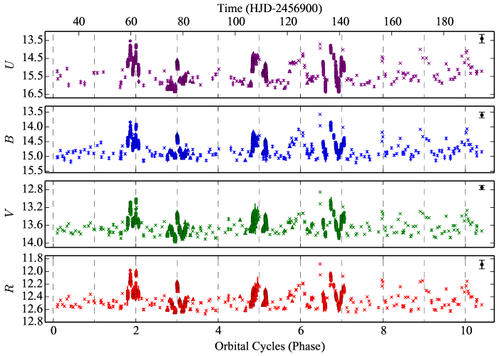
Figure 1.— DQ Tau $UBVR$ lightcurves plotted against (arbitrary) orbital cycle number. LCOGT, ARCSAT, and WIYN 0.9m data are represented as $\times$, circle, and triangle symbols, respectively. ARCSAT data are transformed from SDSS to Johnson filters. Vertical dashed lines mark periastron passages. Note difference in the y-axis scale for different filters. Large error bar in the top right of each panel represents the systematic error in our photometric calibration. (A machine-readable table of the data presented in this figure is available in the online journal.)

Near-simultaneous LCOGT and high-cadence observations provide the opportunity to directly test the agreement of our calibration between datasets. Comparing observations made within 20 minutes of each other (typically 6), the LCOGT-HDI and LCOGT-S2KB mean offsets agree to less than the uncertainties quoted in Pickles & Depagne (2010) for each filter. The LCOGT-ARCSAT offsets are larger, owing to the additional transformation, but are still modest; 0.10, 0.20, 0.10, 0.02 mag for the $UBVR$ transformed magnitudes, respectively. A final offset was applied to match zero-point variations to the HDI dataset from which the apparent magnitudes are initially derived. Offsets were first calculated for overlapping HDI-LCOGT data and then extended to the WIYN 0.9m and ARCSAT datasets (overlapping with LCOGT).

The systematic errors involved in our calibration procedure are much larger than the random error on any given point and the random errors are small compared to the intrinsic variability observed. To remain cognizant of the systematic errors however, we propagate them through each step of our analysis and present them as the black error bar in the top right corner of Figures 1, 6, 8, and 10.

A machine-readable table providing the epoch of observation (Heliocentric Julian date), zero-point corrected apparent magnitude, random magnitude error, and observing facility for each of the $UBVR$ filters can be found in the online journal associated with Figure 1.

3. DETERMINING OPTICAL EMISSION MECHANISMS

The optical emission from accretion and from stellar flares is dominated by a combination of Balmer continuum emission and blackbody radiation. During accretion, the flow of disk material along magnetic flux tubes approaches free-fall velocity (supersonic) toward the stellar surface creating a standing shock above the photosphere. Optically thin material in the post-shock region is responsible for a majority of the blue-optical emission in the form of Balmer continuum. Beneath the post-shock region, the photosphere is radiatively heated creating excess blackbody emission from a hot-spot (Calvet & Gullbring, 1998). Hot-spot temperatures have been modeled ranging from 6500 to 10500 K for late M spectral type stars ($\sim$3000 K photospheric temperatures) with most temperatures in the 8000 to 9000 K range (Herczeg & Hillenbrand, 2008).

During a stellar flare, mass-loaded magnetic field lines in the chromosphere or corona develop unstable configurations, leading to magnetic reconnection events that accelerate charged particles towards the footpoints of the new magnetic configuration. In the thick-target electron beam model used to describe solar and stellar flares (Brown, 1971), these relativistic particles interact with the chromosphere and photosphere where they deposit their energy creating a white-light excesses (Allred et al., 2006). While the mechanism by which mechanical energy is converted into radiative energy remains an open question, most solar/stellar flares follow this general model (Fletcher et al., 2011, and references therein). Observationally, the blackbody component of stellar flares dominates over Balmer continuum at the flare peak where hot-spot temperatures range between 10000 and 14000 K, reducing to 7000 to 10000 K in the decay phase (Kowalski et al., 2013). The higher blackbody temperatures compared to accretion result from energy deposition directly into the photosphere by the electron beam rather than from radiative heating (Kowalski et al., 2015).

While both accretion and flares emit optical light by depositing energy and mass into the stellar surface, the timescale, morphology, and detailed SED of each processes variation can be distinguished with high-cadence, multi-color optical photometry. Accretion is observed to naturally occur in bursts above a steady accretion rate lasting days at a time without a consistent lightcurve morphology (Stauffer et al., 2014). This timescale may be related to the time for instabilities to develop at the disk-magnetosphere interface (Kulkarni & Romanova, 2008; Ingleby et al., 2015).

Stellar flare morphologies on the other hand have been extensively characterized in the case of active M dwarfs, through high-cadence, uninterrupted observation with the Kepler space telescope. Most flares ($\sim$ 85%) exhibit the “classical” morphology consisting of an impulsive-rise followed by an exponential-decay (Davenport et al. 2014; their Figure 3). The ratio of rise-to-decay times varies from $\sim$0.05 to 1, with rise times typically shorter than 10 minutes. Flares also come in non-classical flavors: “complex” or “hybrid”, a superposition of multiple classical flare events, and “gradual” or “slow”, which are less impulsive (Kowalski et al., 2013; Dal & Evren, 2010). Regardless of the flare type, the rise-times are generally less than 1 hour. For reference, the longest optical flare observed on any star (M dwarf, pre-MS, or RS CVn) occurred over $\sim$10 hours and took $\sim$30 minutes to rise (Kowalski et al., 2010, YZ CMi).

We focus on M dwarf flares because the combination of being intrinsically faint (making it possible to detect small flares) and ubiquitous in the galaxy has made them the subject of the most extensive flare studies to date. The observed temporal and morphological characteristics, however, are consistent with the more limited studies of stellar flares on pre-MS stars (Fernández et al., 2004), making them suitable for comparison with DQ Tau. Pre-MS stars appear only to differ in that they have typical flare energies that are a factor of 100 (or more) larger than M dwarfs.

The difference in color between accretion and stellar flares is more subtle than that of the timescale and morphology, especially when only considering the coarse wavelength information presented here ($UBVR$). In general, the peak emission from a stellar flare is bluer than accretion radiation due to the strong, high-temperature blackbody component. As the flare decays, however, this distinction in color becomes less apparent.

To access the physical mechanism behind the broadband variability seen in DQ Tau, we investigate the morphology, timescale, color, and energy associated with brightening events. First, the qualitative aspects of the lightcurve morphology and timescale of variation are compared to long-term, space-based campaigns monitoring accreting young stellar objects and active M dwarfs. Before characterizing the properties of accretion in Section 4, we define quantitative limits for the detection of flares, characterize the color, timescales, and energy of those that are detected, and place limits on their contribution to the total optical variability. Finally, we place our results in the context of the colliding magnetospheres scenario.

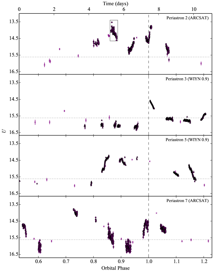
Figure 2.— DQ Tau high-cadence, U-band lightcurves highlighting the rise and decline over the course of days near periastron passage. Vertical dashed lines mark periastron passage. Horizontal dotted lines mark the quiescent brightness. Periastron number in relation to Figure 1 is provided in the top right of each panel along with the source of the data. LCOGT observations are $\times$ symbols. The light gray box in the top panel marks the region plotted in Figures 4 and 5.

3.1. Lightcurve Characteristics

Figure 1 presents our full DQ Tau, $UBVR$ lightcurves covering 10.3 orbital periods ($\sim$163 days). LCOGT observations are presented as $\times$ symbols with ARCSAT and WIYN 0.9m observations shown with circles and triangles, respectively. The bottom x-axis is an arbitrary orbital cycle number chosen to set the first observed periastron passage to 1. Below, we refer to brightening events using the cycle number as it is presented in this figure. (The top axis displays Heliocentric Julian days.) Each periastron passage is shown with a vertical dashed line. The y-axis scale of each panel is set to match the variability of each filter and differs greatly with photometric band. As expected in either accretion or flare events, the bluest filters display the largest variability; $>$3 mag in $U$ while $<$1 mag in $R$.

Focusing on the $U$-band lightcurve in Figure 1 (our most sensitive diagnostic of photospheric hot-spots, whether from accretion or flares), brightening events of varying complexity and amplitude are seen around each periastron passage. The duration of these events varies and can be as long as half the orbital period. A significant amount of variability is also seen outside of periastron, especially near certain apastron passages (e.g. orbital cycles 6.5, 8.5, and 9.5).

Comparing our $V$-band lightcurve with that of Mathieu et al. (1997), we find consistent results with brightening events occurring around many, but not all, periastron passages. Simultaneous observations in $U$-band, however, reveal that “quiescent” $V$-band periastron passages do indeed have a detectable $U$-band enhancement, due to the smaller contribution from the stellar photospheres and a larger contribution from accretion luminosity at shorter wavelengths. With the large range in time presented in Figure 1, the detailed structure of brightening events are hard to discern but already it is clear that some periastron passages display short, bursty events (orbital cycles 3 and 8), while others display a prolonged elevated state (orbital cycles 5, 6 and 9).

Figure 2 provides an expanded view of our high-cadence $U$-band observations. Each panel presents a different periastron passage listed in the top right, with vertical lines denoting the time of closest approach. Horizontal dotted lines mark the quiescent $U$-band value from orbital phases $\phi$=0.2 to 0.4 (consistently the quietest phase of the orbit, see Figure 7 for reference). These data highlight the complex structure of periastron brightening events showing variability in the morphology, scale, and onset of the event. While variability is seen on a variety of timescales, the underlying large scale evolution takes place over days rather than hours. Each periastron passage observed with high-cadence photometry shows increases above the quiescent level for tens of hours if not days at a time.

Recent space-based campaigns monitoring the variability of accreting young stellar objects and magnetically active M dwarfs provide a wealth of data against which to compare our high-cadence observations. The CoRoT space telescope monitored the star-forming region NGC 2264 for $\sim$40 days continuously at a 512-second cadence, revealing a myriad of complex variability trends (Cody et al., 2014). Comparing our $R$-band observations to the $CoRoT$ $R$-band (white-light) lightcurves, we find many similarities with the class of objects defined as “bursters” (Stauffer et al. 2014; their Figure 1, right panels). These objects make up the dominant lightcurve class of stars with large UV-excesses and are interpreted as episodic bursts of accretion evolving over days at the few tenths of a magnitude level in $CoRoT$ $R$. The variable morphology of these events as well as their amplitude and timescale, support an accretion dominated interpretation of the observed optical variability.

We also compare our lightcurves to the Hawley et al. (2014) study of active M dwarfs using $Kepler$, minute-cadence data. Variability in these stars is dominated by sinusoidal star-spot modulations with sharp enhancements from flares. Flares of this type would appear as near-vertical brightening events in Figures 1 and 2 while the observed enhancements are smoother in nature.

The color of the variability also points to accretion. The observed $R$-band increases are on the order of $\sim$0.5 mag with $U$-band excesses of $\sim$2 mag. This color is redder than what is typical of stellar flares at their peak. Flares with peak $R$-band enhancements of 0.5 mag are rare and accompanied by $U$-band components of $>$4 mag (Hawley & Pettersen, 1991; Davenport et al., 2014). Figure 3 presents the extinction corrected $U$-$R$ excess color vs $U$-band excess above a photospheric model (described in Section 4). Most data do not reach the extremely blue $U$$-$$R$ colors typical of large flare peaks ($U$$-$$R$ $\sim$ 3.5).

We explore the presence of flares in more detail in the following section but in general, conclude that large scale changes in the accretion rate are the most plausible source of optical variability based on the morphology, timescale, amplitude, and color of the events.

Figure 3.— Extinction corrected $U$–$R$ color-magnitude diagram of emission above the stellar photosphere. Encircled points highlight candidate flares from high-cadence lightcurve analysis. The bluest point observed in $U$–$R$ is the peak emission of “Flare 1” presented in Figure 5 (see text). (Extinction and template determination discussed in Section 4.)

3.2. Stellar Flares

Although accretion processes appear to dominate the large-scale optical variability on day timescales, we also investigate our nightly, high-cadence lightcurves to determine the contribution from stellar flares. Based on the empirical M dwarf flare behavior described above, we develop a flare finding scheme aimed at detecting impulsive brightening events on timescales of tens of minutes in our $U$-band, high-cadence lightcurves. Our detection scheme is as follows: for each $U$-band observation the median value of data and its error within the prior 60 minutes is computed (typically 12 to 20 points given our average cadences on each telescope/detector combination). Points falling 10 times above the median error are then visually inspected as possible flares. This conservative value is taken to compensate for the large underlying variability from accretion. Our flare detection threshold is adaptive in this case and can range from $\Delta U$=0.04 to 1.58 with a median value of 0.32 mags. Using a shorter averaging window of 30 minutes recovers the same results.

Following this procedure, three groups of points fall above our 10$\sigma$ threshold. The first two are short-timescale events we select as flare candidates and discuss in detail below. The third comes from the steep rise prior to periastron passage 5 (Figure 2, third panel, orbital phase $\sim$0.83). While a spectacular event in and of itself, rising more than 1 mag in $U$ over the course of $>$9.5 hours, we do not classify it as a flare given the relatively long timescale over which it is evolving.

Figure 3 presents the $U$–$R$ color-magnitude diagram of emission above the stellar photosphere. Data from the two candidate flares are over-plotted with blue circles. The bluest point observed occurred during the peak of the first candidate flare and is significantly bluer than other measurements that are attributed to accretion. This aligns with our expectation that the peak brightness of a stellar flare will be bluer than the emission from accretion. Most of the rise and decay phase, however, are indistinguishable in color space from the rest of the optical (accretion) variability.

Figure 4 presents the night of high-cadence data in which our candidate flares are detected. The fact that these two events fall close together in time (partially overlapping) is not necessarily a concern given that there is evidence for sympathetic flaring (flares triggering subsequent flares) on low-mass stars (Panagi & Andrews, 1995; Davenport et al., 2014) and the Sun (Pearce & Harrison, 1990). To provide context within the large-scale variability of DQ Tau, these data are highlighted in the top panel of Figure 2 with a light gray box. In an attempt to characterize the emission from these events alone, we fit a cubic spline to regions of the lightcurve devoid of flares in order to remove accretion variability. The fit is shown as the gray dashed line in Figure 4. Subtracting this crude model and converting to normalized flux results in Figure 5.

The first event in Figure 5, “Flare 1”, has the morphology of a classical flare. The red line over-plots an empirical classical flare template from Davenport et al. (2014). Constructed from 885 classical white-light flares on the active M dwarf GJ 1243 observed with $Kepler$, this flux normalized model is broken into a rise and decline phase that depends on the event timescale, $t_{1/2}$, the time spent above half the peak flux. A 4th-order power series in $t_{1/2}$ describes the rise phase and a sum of two exponentials describes the decline. We do not fit the template to our data in a $\chi^{2}$ sense, but over-plot the template using the measured $t_{1/2}$ value and an amplitude normalization. The agreement is not perfect but given the uncertainty in the background subtraction, we find it to be reasonable evidence that this event is a flare from a magnetic reconnection event.

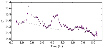
Figure 4.— ARCSAT U-band lightcurve during one night of observation in which two flares are present. The gray box in the top panel of Figure 2 shows the location of these data with respect to orbital phase and the rest of the observing run. The gray dashed line displays a cubic spline fit to regions of the lightcurve devoid of flares.

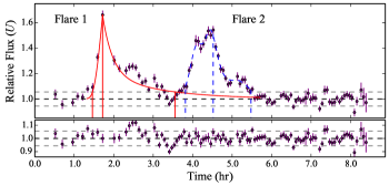
Figure 5.— Lightcurve from Figure 4 plotted as relative flux above the background accretion variability model. The red curve displays the classical flare template of Davenport et al. (2014). Vertical red lines mark the beginning, peak, and end of the flare. The blue curve is a cubic spline fit to the classical flare subtracted lightcurve. Vertical blue dashed lines mark the beginning, peak, and end of the gradual flare. The bottom panel presents the residuals from model subtraction. Horizontal gray dashed lines in both panels mark the standard deviation of data devoid of flares after subtraction of the accretion model.

The second event during this night, “Flare 2”, does not have the classical flare morphology but may be a slow or gradual flare. Although, our cadence may not be high enough to decompose multiple small classical flares events if it were instead a hybrid or complex flare. Without an empirical model for non-classical flares to compare against, we fit a cubic spline (blue curve in Figure 5) to the accretion and classical flare subtracted data.

In addition to the morphology and timescale arguments above, we make a quantitative comparison of the flare energy in the $UBV$ filters to flares observed on other pre-MS stars. We determine the rise and decay times for each flare where our flare templates exceed the non-flaring standard deviation (top dashed line in Figure 5; location of start, peak, and end times are marked with vertical lines). The flare energy is then computed with a trapezoidal integration of the excess emission above our accretion model (dashed line is Figure 5) assuming a distance of 140pc and $A_{V}$=1.5 (see Section 4). Table 2 presents their temporal characteristics from the $U$-band lightcurve and total energy in the $UBV$ filters. Error in the energy comes from applying the maximum and minimum offsets of our photometric systematic error. The derived energies in each filter fall within the spread of flares observed on other pre-MS stars ($2\times 10^{34}<E_{U}$(ergs)$<1.1\times 10^{36}$; Gahm, 1990; Fernández et al., 2004; Koen, 2015) and the ratio of energy between each filter agrees with the trend seen on pre-MS stars as well as M dwarfs (Lacy et al., 1976; Gahm, 1990). This result provides further evidence for a magnetic reconnection origin of these events.

These two flares were the only events in our high-cadence lightcurves that had the amplitude and timescale typical of magnetic reconnection as we understand them from low-mass dwarfs and pre-MS stars. To quantitatively compare the timescale of our flares to the large-scale variability, we measure the $t_{1/2}$ values of the 10 largest brightening events observed at high-cadence. Using the quiescent brightness level shown in Figure 2 as the baseline, we find an average $t_{1/2}$ value of 21.7 hours with the shortest being 2.5 hours. These values are an order of magnitude longer than those calculated for the flares in Table 2.

Table 2Flare Characterization Summary

Parameter	Flare 1	Flare 2
$t_{1/2}$ (min)	23.9	41.6
Rise Duration (min)	15.4	42.4
Fall Duration (min)	110.2	57.4
$\Delta U$ (mag)	0.55	0.47
$U$-band Energy ($10^{35}$ ergs)	$2.2\pm 0.5$	$1.6\pm 0.4$
$B$-band Energy ($10^{35}$ ergs)	$2.1\pm 0.4$	$1.0\pm 0.2$
$V$-band Energy ($10^{35}$ ergs)	$1.8\pm 0.2$	$0.5\pm 0.1$

Note. — Temporal measurements from $U$-band lightcurve.

Lastly, to determine the fraction of our data in which flares are present, we first calculate the amount of time in which our data are capable of detecting flares. Hawley et al. (2014) find that a majority of flares are less than 2.5 hours in duration. Setting this as the minimum duration of continuous monitoring (with data gaps less than 30 minutes) required to detect flares, 141 hours of “flare coverage” are obtained. Within this window, only 4.1 hours contain flares at an average level of $\Delta U$$\sim$0.32, corresponding to $\sim$3%. Here we have assumed a perfect detection efficiency above the detection threshold as each event is visually inspected and characterized, finding it in good agreement with flares on other pre-MS stars. With that in mind, this value should be taken as a lower limit on the temporal flare contribution given our variable detection threshold. Small flares that would go undetected in our data evolve quickly however, and would not contribute significantly given the $\sim$3 magnitude $U$-band variations observed in the system. We also note that the fraction of time spent flaring derived above is from observation near periastron alone. Our data provide no information on the occurrence of flares near apastron or if any orbital-phase-dependence exists.

We conclude that flares play a very small roll in the amplitude and temporal nature of DQ Tau’s variability, and that the broadband variability is due to a variable accretion rate. For the remainder of our discussion we remove the two flares using the models described above (the residuals of which are shown in the bottom panel of Figure 5) and attribute all remaining variability to changes in the accretion rate.

3.3. Colliding Magnetospheres

Here we consider whether the detection of flares near a periastron passage of DQ Tau might be indicative of magnetic reconnection events in colliding magnetospheres. In this scenario, the large-scale magnetic fields of both stars interact during periastron approach (bringing the stars from $\sim$43 to 12 $R_{\star}$) leading to unstable magnetic configurations and reconnection in the case of field lines with opposing polarity (see Adams et al. 2011).

Evidence for colliding magnetospheric reconnection in DQ Tau comes from Salter et al. (2010) who find recurrent, mm-wave synchrotron enhancements during three out of four observed periastron passages. With only 8 to 16 hours of observation per periastron passage, the consistency of radio flares points to inter-magnetospheric reconnection being a commonplace event near periastron. The largest of these events reached a peak luminosity of $\sim 10^{28}$ ergs s^-1 at 2.7 mm (115 GHz; 1 GHz bandpass) and while it was not observed through its return to quiescence, the event was modeled with a $\sim$30 hr duration. Radio flares of this amplitude have been observed on the weak-lined T Tauri star (WTTS) binary V773 Tau (Massi et al., 2002, 2006), which were also attributed to colliding magnetospheres. Both, however, are an order of magnitude more luminous than largest radio events observed on active M dwarfs (Osten et al., 2005) or RS CVn binaries (Trigilio et al., 1993). If optical events similar to stellar flares accompanied these events at amplitudes that scale with the radio component, our observations would easily detect them given the sensitivity to impulsive brightening events derived above.

While we have assumed that magnetic reconnection between colliding magnetospheres is capable of creating an optical, stellar-flare-like counterpart, determining the detailed characteristics of an optical counterpart to radio events of this scale is difficult. Some of the most extensive simultaneous radio and optical monitoring has been on active M dwarfs. During flares the optical component is seen to evolve on a much shorter timescale than the radio counterpart (Osten et al., 2005; Butler et al., 2015). The prolonged radio decay is attributed to magnetic mirroring near footpoints where field lines converge, increasing the field strength, and reflecting synchrotron producing electrons (e.g. Aschwanden et al. 1998). This effect may have a large impact on magnetic reconnection events far from the stellar surface. The efficiency of magnetic mirroring depends on the ratio of the field strengths that a particle experiences which, for DQ Tau, assuming a simple dipole, would correspond to $\sim$245 from 6.3$R_{\star}$ (midpoint between stars at periastron) to the stellar surface. In solar flares where the site of reconnection is in the chromosphere or corona, this ratio is typically measured as 2, or less (Tomczak & Ciborski, 2007; Aschwanden et al., 1998).

Moving the site of reconnection further from the surface of the stars also raises concerns of synchrotron radiative losses and the potential for collisional losses with intervening circumstellar material that prevents accelerated electrons from reaching the chromosphere. If the energy from magnetic reconnection remains confined or lost to other processes it will prevent the conversion of mechanical energy to an optical counterpart at the stellar surface. Salter et al. (2010) present some simultaneous optical photometry during the decay phase of one of their radio flares which also shows a general decaying behavior (their Figure 7). While the match between the optical and radio morphology is compelling, this behavior is not seen in standard solar/stellar flares.

Aside from lightcurve morphology, we also compare the energy of optical and radio brightening events to the available magnetic energy budget. Assuming quasi-static, anti-aligned dipole fields, Adams et al. (2011) estimate the magnetic interaction energy available for reconnection events as a function of the stellar radius, the surface magnetic field strength, and apastron-to-periastron separation (their Equations 13 and 14). The interaction energy is derived from the difference between the lowest energy magnetic field configurations at periastron and apastron. Energy in this model is provided by the orbital motion which compresses the fields and is only a fraction of the total magnetic energy stored in the fields.

Adopting a surface dipole field strength of 1.5 kG and the parameters listed in Table 1, DQ Tau has an available interaction energy of $\sim 10^{35}$ ergs (only $\sim$1% of the combined magnetic energy beyond an interaction distance of 6.3$R_{\star}$ for each star). Integrating a synchrotron source function matching the observed 90 GHz flux density from 0 to 90 GHz for a range of power-law electron energy distributions (1.1 to 2.9), we find energies ranging from 0.4-6.7$\times 10^{35}$ ergs, assuming a 6.55 hr $e$-folding decay timescale (Salter et al., 2008, 2010). For comparison, trapezoidal integration of our photosphere-subtracted, flux-calibrated observations produces an average of $\sim$10³⁸ ergs emitted in the combined $UBVR$ filters during periastron passage ($\phi=0.7$ to 1.3), a factor of 10³ more than the available magnetic energy budget.

Based on the multi-day variability of optical brightening events, the excess of optical energy released near periastron when compared to the colliding magnetosphere energy budget, the paucity of classical optical flare events (for lack of a better model), and the favorable conditions for magnetic mirroring, we conclude that reconnection events from colliding magnetospheres do not contribute significantly to the periodic luminosity increases in our optical lightcurves. The optical flares that are present do have energies that agree with the colliding magnetosphere energy budget but, they are also typical of flares on single pre-MS stars, are less regular than radio events, and occur at a relatively wide stellar separations ($\sim$24$R_{\star}$). These flares may very well be the result of magnetic reconnection on the surface of one of the two stars. Simultaneous optical and radio observation will be required, however, to make a definitive statement on their origin.

4. Characterizing Accretion

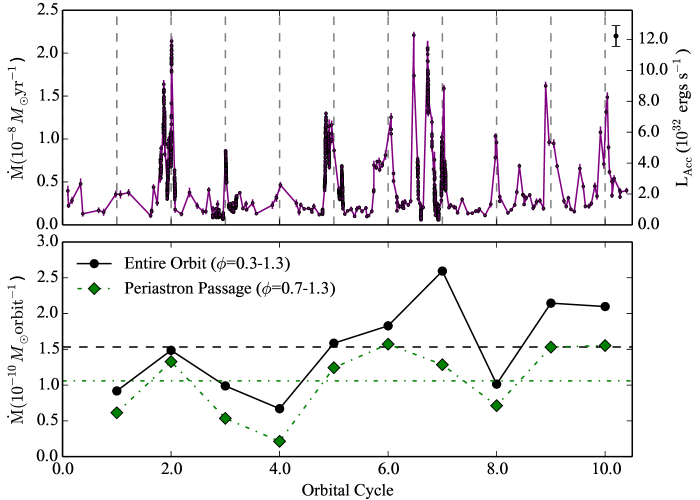
Figure 6.— Top: Accretion rate (left axis) as a function of orbital cycle. Right axis displays the corresponding accretion luminosity. Dashed vertical lines mark periastron passages. Bottom: Integrated mass accreted per orbit. Black circles represent the mass accreted per full orbital period (orbital phases $\phi$=0.3 to 1.3). Green diamonds represent the mass accreted per periastron passage (orbital phases $\phi$=0.7 to 1.3). Horizontal dashed and dot-dashed lines mark the average orbital and periastron accreted masses, respectively.

A measurement of the mass accretion rate can be made by determining the excess emission above the stellar photosphere(s) resulting from accretion. This requires an estimate of the underlying spectral type and extinction in the absence of accretion. We determine these properties following the method described in Herczeg & Hillenbrand (2014). These authors compute a library of low-resolution, pre-MS spectral templates from a grid of 24 flux-calibrated WTTS spectra, spanning spectral types K0 to M9.5. Empirical templates have the advantage over synthetic spectra in that they include chromospheric emission (see Ingleby et al. 2011) and provide more accurate colors for these typically, highly spotted photospheres (e.g. Grankin et al., 2008; Alencar et al., 2010). Templates are fit to the spectra of accreting CTTSs modifying the intrinsic luminosity, extinction, and additive accretion continuum level as free parameters. Cardelli et al. (1989) extinction curves are used assuming $R_{V}$=3.1 and the accretion continuum is modeled as a constant flux value across wavelength. As noted above, the true accretion spectrum has structure from the Balmer jump and emission lines; however, the fits here only include wavelength regions redward of 4000Å and exclude emission lines. Within these continuum-dominated windows, a flat spectrum provides an adequate description of accretion while keeping the degrees of freedom minimal. The binary nature of DQ Tau is ignored in this process but as a near equal-mass binary, the combined spectrum of both stars should not differ greatly from that of a single star at low-spectral resolution.

Applying this procedure to a flux-calibrated spectrum of DQ Tau obtained in January 2008 with the Double Spectrograph (Oke & Gunn, 1982) on the Hale 200 inch telescope (originally published in Herczeg & Hillenbrand 2014), we find a spectral type of M0.4 and an extinction of $A_{V}$=1.5. These values agree with the results of Herczeg & Hillenbrand (2014) who quote typical uncertainties of 0.3 spectral type subclasses and 0.3 magnitudes of extinction for (single) M stars. Both measurements also lie in the middle of the values found in the literature (Strom et al., 1989; Kenyon & Hartmann, 1995; Czekala et al., 2016). Even though this work is primarily concered with the relative changes of the accretion rate, the importance of extinction on the derived accretion rate baseline should be noted. The $\pm$0.3 magnitude uncertainty of this method corresponds to a 0.2 dex systematic uncertainty in all accretion luminosities (rates) and flare luminosities (energies).

The WTTS templates extend from 3130-8707Å with a central gap from 5689-6193Å. Before convolving the best-fit template with filter curves we fill this gap in the spectral coverage by finding the best-fit BT-Settl atmospheric model (Baraffe et al., 2015). A best fit is found at a temperature of 3900 K and log($g$) of 4.0, in agreement with Czekala et al. (2016).

With a model for the combined photospheric contribution in DQ Tau, we determine the mass accretion rate by first converting the $U$-band excess luminosity into an accretion luminosity following the empirical relation found by Gullbring et al. (1998):

$${\rm log}(L_{\rm Acc}/L_{\odot})=1.09\ {\rm log}(L_{\rm{\it U_{\rm excess}}}/L_{\odot})+0.98$$ (1)

The $U$-band photospheric luminosity is computed by convolving the template with a $U$-band filter curve (Maíz Apellániz, 2006; Pickles & Depagne, 2010), adopting a distance of 140 pc. This luminosity is then subtracted from the observed, extinction-corrected $U$-band luminosity, providing $L_{\rm{\it U_{\rm excess}}}$.

In these calculations we have ignored the contribution to variability from star-spots. Spot variations on non-accreting pre-MS stars are typically a few tenths of a magnitude in $U$-band (Bouvier et al., 1995). This is much smaller than the observed variability and at a high inclination angle ($\sim$22 degrees), the geometry of hot and cool spot visibility due to rotation should have a small effect.

From accretion luminosities we calculate mass accretion rates using the following formula,

$$\dot{M}\simeq\frac{L_{\rm Acc}R_{\star}}{GM_{\star}}\left(1-\frac{R_{\star}}{R_{\rm in}}\right)^{-1},$$ (2)

where $R_{\rm in}$ is the magnetospheric truncation radius from which accreting material free-falls along field lines. The value of $R_{\rm in}$ depends on the strength of the magnetic field and the ram pressure of accreting material. In the binary environment, where mass flows are predicted to be highly variable and phase dependent (ML2016), the conditions of accreting material are likely not well described by a single value of $R_{\rm in}$. As we discuss below, the ram pressure of accreting material is likely highest near periastron. If this behavior corresponds to smaller $R_{\rm in}$ values, a constant value of $R_{\rm in}$ will underestimate the accretion rate near periastron and overestimate it at times of low accreting ram pressure (presumably apastron). Without a model for the time variable interaction of the magnetic field with circumstellar material, we resort to the canonical single star value of $R_{\rm in}=5R_{\star}$ (Gullbring et al., 1998), even though it is less physically motivated in this case. Fortunately, the mass accretion rate is fairly insensitive to $R_{\rm in}$ (a factor of 2 decrease in $R_{\rm in}$ corresponds to a factor of 0.6 in the mass accretion rate). Given these uncertainties, accretion luminosity measurements are also included in Figures 6, 7, and 10.

Following this procedure we calculate mass accretion rates ranging from $5.9\times 10^{-10}$ to $2.2\times 10^{-8}M_{\odot}{\rm yr}^{-1}$, in good agreement with measurements from optical and NIR spectra (Gullbring et al., 1998; Bary & Petersen, 2014). The top panel of Figure 6 displays the mass accretion rate as a function of orbital cycle. An increase in the accretion rate can been seen at every periastron passage; at some, the accretion rate increases by more than a factor of 10 from the quiescent value.

The bottom panel of Figure 6 presents the mass accreted over each full orbital period and over each periastron passage. For the full orbit, we define our integration range to be orbital phases $\phi=0.3$ to 1.3 in order to include the entire periastron event. For periastron passages, the integration range is over orbital phase $\phi=0.7$ to 1.3. Black circles and green diamonds mark the full orbit and periastron integrations, respectively, with horizontal lines marking the mean of each. This periastron passage range encloses 60% of the orbital period but has a median contribution of 71% to the total mass accreted per orbital period. Large variability exists, however, with periastron contributions ranging from 49-90% of the total mass accreted per orbital period.

4.1. Periodic Enhanced Accretion

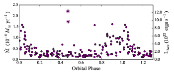
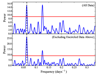
Figure 7.— Top: Mass accretion rate (left axis) from LCOGT observations phase-folded about the orbital period. Right axis displays the corresponding accretion luminosity Middle: Lomb-Scargle periodogram of all of the above data. Bottom: Lomb-Scargle periodogram of the above data excluding the two encircles periastron points. In both periodograms the horizontal red line marks the 99% false-alarm-probability and the vertical dashed line is the radial-velocity determined orbital period.

Numerical simulations of the binary-disk interaction predict that in cases of high eccentricity, discrete accretion events should occur near every periastron passage. We test this prediction by performing a Lomb-Scargle periodogram analysis (Scargle, 1982) on the mass accretion rates derived from LCOGT observations. Figure 7 displays the mass accretion rate phase-folded about the spectroscopically determined orbital period in the top panel and the periodogram of those data in the middle panel. The red line in the bottom two panels marks the 99% false-alarm-probability (FAP) determined using a Monte Carlo bootstrap simulation (Frescura et al., 2008).

Even with the large variability present near periastron, typical of accretion in CTTSs, a significant peak is found near the spectroscopic period (marked with the dashed vertical line). We find a period of 15.91$\pm$0.08 days, in good agreement (1.3$\sigma$) with the orbital period. (Periodogram peak errors are calculated by enclosing 68% of a the probability-distribution-function created from a $10^{6}$ iteration Monte Carlo, bootstrap simulation using sampling with replacement in time and $\dot{M}$ (Press et al., 1992).) This spectral peak and the visual inspection of the Figure 6 provide compelling evidence that, just as models predict, pulsed accretion events occur periodically near each periastron passage.

A second significant peak found at half the orbital period is powered by apastron accretion events. Most of the power at this frequency comes from the two closely separated LCOGT observations near orbital cycle 6.5. These two point are encircled in the top panel of Figure 7. (Other apastron accretion examples can be seen at orbital cycles 8.5 and 9.5 in Figure 6.) A periodogram excluding these two points is presented in the bottom panel of Figure 7 where a peak is still present above the 99% FAP. Non-sinusoidal waveforms, like those observed, are capable of producing harmonics above a 99% FAP at integer multiples of the primary frequency. This is potentially the case in the bottom panel of Figure 7 but not in the middle panel where the peak at twice the orbital frequency is the highest of the two. We conclude that apastron accretion events are quasi-periodic, occurring at generally lower amplitudes and with less consistency when compared to periastron accretion events. Apastron accretion events are not predicted by the binary pulsed accretion theory and are discussed further in Section 4.3.

In addition to the presence of enhanced periastron accretion, the morphology and timing of the observed accretion events also provide a test of numerical simulations. Given that large variability exists from orbit to orbit we create an orbit-averaged accretion rate as a function of orbital phase. First, as to not over-weight the orbital periods with high-cadence observations, while still making use of the morphological information they provide, a linear interpolation of the mass accretion rate is computed and re-sampled at our average moderate-cadence rate (20 times per orbital period). The median value from 10 orbital periods is then calculated in phase bins of $\phi=0.05$ (10 measurements per bin) resulting in the orbit average accretion event profile in Figure 8. The error bars at each bin signify the standard deviation within that bin from orbit-to-orbit. On average, accretion rates increase by a factor of $\sim$5 above quiescence at periastron ($\phi=0.95$ to 1.05) with a mostly symmetric rise and decay about periastron.

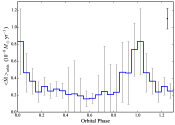
Figure 8.— Orbit-averaged (median) mass accretion rate from 10 orbital cycles of observation. Error bars are the standard deviation within each phase bin. Black error bar in the top right corner denotes the propagation of the systematic error of our photometric calibration.

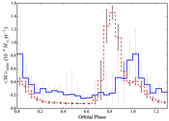
Figure 9.— Orbit-averaged (median) mass accretion rate from 10 orbital cycles of observation and simulation in blue solid and red dashed lines, respectively. Error bars are the standard deviation of the accretion rate within each phase bin. Simulation results come from Muñoz & Lai (2016) 2D hydrodynamical models.

To compare our results directly with numerical simulations, we create an orbit averaged mass accretion rate from the ML2016 2D hydrodynamical models of binary accretion (D. Muñoz, private communication). These models are novel in that they utilize the adaptive mesh refinement code AREPO (Springel, 2010), extend out to radii of 70$a$, and run for $>$2000 orbital periods reaching full relaxation from the initial conditions out to a radius of $\sim$5$a$ in the CBD. Using the results from 10 orbital periods of their scale-free, eccentric ($e=0.5$), equal-mass binary simulation (similar to DQ Tau; $e=0.568$; $q=0.94$), we perform the same averaging scheme used on our observations. The simulated accretion rate is normalized by matching the average accretion rate per orbital period to our observations (Figure 6). Figure 9 presents a comparison of the model and data which, to first order, shows remarkable agreement given the limited input physics of the model (only gas physics and gravity). Both show significantly enhanced accretion from $\phi\sim 0.8$ to $\sim$1.1.

In detail however, the model and data differ in the specific morphology of the average accretion event, the orbital phase of peak accretion, and the consistency of both compared to the observed variability (apparent when comparing the variability within each phase bin from the model to observations). Exploring these differences acts to highlight the important ingredients missing from numerical simulations. In the ML2016 simulations each star develops a tidally truncated circumstellar disk that extends down to the stellar radius where mass is deposited. With viscous accretion timescales as short as 20 orbital periods for disk of this size, circumstellar disks are replenished each orbital period by a circumbinary accretion stream. This process acts as an accretion buffer that organizes the incoming material before it reaches the stars. Bursts of accretion in this case arise not from accretion stream material impacting the stars themselves but from companion-induced tidal torques on the circumstellar disks during periastron approach. These gravitational torques induce non-axisymmetric structures in the circumstellar disks (spiral arms) that dissipate orbital energy, funneling material inward.

In the case of DQ Tau however, strong magnetic fields may truncate the inner edge of the circumstellar disks, potentially to the point that no stable circumstellar orbits exist. Dynamical outer truncation radii for binary circumstellar disks are $\sim$0.2$a$ or $\sim$5.6$R_{\star}$ for DQ Tau’s orbital parameters (Eggleton, 1983; Miranda & Lai, 2015). As discussed above, the inner magnetospheric truncation radius is likely to vary with the conditions of incoming material but a typical single-star value is $R_{\rm in}\sim 5R_{\star}$, essentially the same as the dynamical truncation. In this case, the efficency of circumstellar material to buffer accretion streams would be greatly reduced leaving accretion events more subject to the timing and extent of material contained within each accretion stream.

This scenario explains the orbit-to-orbit consistency in amplitude and morphology the ML2016 simulation shows over our observations. The fact that the simulated accretion rates rise and peak well before ours is likely also due to the size/existence of circumstellar disks. If the material constituting DQ Tau’s periastron accretion events is provided by the accretion stream of that orbital period alone, there may be no circumstellar material laying in wait to be torqued by the companion star, delaying the onset of accretion. In addition, periastron passages 5 and 7 (Figure 6), for instance, display discrete accretion events at orbital phases 1.18 and 0.72, respectively, where companion-induced tidal torques are likely insignificant given the stellar separation.

It is possible that we have confirmed the observational predictions of numerical simulations without, necessarily, the same dominant physical mechanisms at play. Simulations including treatments of magnetism and radiative transfer may be required for a more in-depth comparison with short-period systems like DQ Tau. Long-period binaries where the magnetospheric inner truncation radius is less significant may be well described by these models.

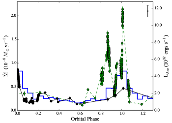
Figure 10.— The mass accretion rate (left axis) of the most active and passive orbital periods. The green and black data are from orbital cycles 2 and 4, respectively. The blue histogram is orbit-averaged accretion rate from Figure 8. The right axis present the corresponding accretion luminosity.

4.2. Accretion Variability

The orbit-averaged accretion rate above provides definitive evidence that bursts of accretion primarily occur near periastron, consistent with the predictions of the binary pulsed accretion theory. However, the orbit-averaged accretion rate provides a very poor description of the behavior in a given orbit. Figure 10 highlights this variability, presenting one of the more active and passive orbital periods.

Other than occurring primarily near periastron, accretion events vary in amplitude, duration, and morphology. Our high-cadence observations reveal that, rather than a single rise and decay across periastron, accretion occurs in discrete, short-lived events (Figure 10). In some sense, this behavior is not surprising given the large amount of variability seen in single CTTSs (Rucinski et al., 2008; Cody et al., 2014; Stauffer et al., 2014). The Kulkarni & Romanova (2008) 3D MHD simulations of Rayleigh-Taylor unstable accretion, for instance, provide a good qualitative match to the bursty and quasi-period nature of accretion on single CTTSs.

Inspection of the bottom panel of Figure 6 shows a factor of $\sim$5 variability (min-to-max) in the mass accreted per orbital period. For reference, the ML2016 simulation only vary by $\sim$10% from orbit-to-orbit. The source of this variability must come from either changes in the amount of CBD material supplied from one orbit to the next or changes in the efficiency at which the stars drain their reservoirs of material. If we assume the amount of material brought in through accretion streams is the same for every orbit and only the efficiency at which the stars accrete changes, we would expect orbital periods with low accretion to be followed by those with high accretion, fueled by “leftover” material. Although only 10 orbital cycles are observed, there does not appear to be any obvious connection between the mass accreted from one orbital period to the next.

If instead, each star accretes a majority of its bound material within an orbital period (the case if little/no stable circumstellar material exists), variability in the mass accreted per orbit would reflect variability in the mass supplied by the circumbinary streams. The time-variable nature of gravitational perturbations from an eccentric orbit creates a dynamic and unstable region near the CBD edge that could supply the inhomogeneities required to explain our observations. The ML2016 CBDs, for instance, develop asymmetries that precess around the central gap as well as over-densities that grow, becoming unstable, and fall inward.

While changes in the stellar accretion efficiency and stream mass are likely both at play, we find the observed variability is most easily explained by assuming a significant portion of the circumstellar material is truncated near the star by magnetic fields, greatly inhibiting the ability to buffer, or hide, variability in accretion streams. This is supported by the variability in the accreted mass from orbit-to-orbit as well as the bursty and varied orbital phases of the near-periastron accretion events. The discrete nature of the observed accretion events (Figure 10) may also indicate an inhomogeneous nature to the material within a given stream that provides a non-steady flow of material to the stellar surface(s).

Changes in the magnetic field topology almost certainly plays a role in accretion variability as well. With large-scale magnetic reconnection events and time-variable ram pressure from accreting material, the state of the magnetic fields is largely unknown. We find it unlikely that the magnetic field alone could be responsible for suppressing the accretion rate to the degree that is observed in some orbital cycles, but it may affect the ability of the stars to capture stream material, alter the efficiency at which they drain the reservoir of circumstellar material, and foster the bursty nature of the observed accretion.

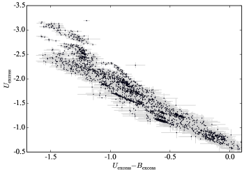
Figure 11.— $U$–$B$ color of the excess accretion luminosity versus the $U$-band excess above the stellar photosphere (flares removed). The $U$-band excess luminosity is a proxy for the mass accretion rate. For given $U$-band excess a variety of $U-B$ excess colors are present.

In addition to variability in the accretion rate itself, the spectral characteristics of the accretion luminosity is also variable. Figure 11 displays the color-magnitude diagram of the $U$-band excess emission versus the $U$–$B$ excess color. Here we see complex behavior where the $U$–$B$ excess color is not simply a function of the $U$-band excess, a proxy for the mass accretion rate. For a given $U$-band excess, a wide range of $U$–$B$ excess colors exist pointing to different physical conditions of emitting material for a single $\dot{M}$. Tightly grouped streaks in the color-magnitude diagram correspond to individual nights of high-cadence observation where we can see changes in not only the accretion rate, but also the conditions of accretion.

Calvet & Gullbring (1998) have modeled the emission of accreting CTTSs in the magnetic paradigm where, for a given mass and stellar radius, the emergent emission from an accretion column is set by its energy flux, $\rho v^{3}/2$, and surface filling factor (also see Ingleby et al. 2013). Increasing the energy flux of these models corresponds to an increase in the total emission, specifically blueward of the Balmer jump which, centered in the $U$-band, is likely the dominant source of $U-B$ excess color variability. Physically, this would require either a change in the density of the accreting material, its velocity, or the size of the accretion site. All three are likely to be changing in DQ Tau. Inhomogeneities in accretion streams could affect the density of incoming material while simultaneously compressing the magnetic field to small $R_{\rm in}$ values which would correspond to small free-fall velocities (Equation 2). This variable accretion scenario is also likely to form Rayleigh-Taylor instabilities leading to unstable accretion flows which can increase the covering fraction of accretion sites (Kulkarni & Romanova, 2008). It is also possible that both stars are accreting simultaneously under different conditions.

While our four-color photometry does not provide the spectral leverage to estimate changes in the energy flux or physical size of accretion sites, we note that when comparing the slope of the $U$-band lightcurve to the excess $U$–$B$ color, the rise of accretion events are consistently bluer that the decay. We interpret the bluer color as a larger emission blueward of the Balmer jump in the accretion spectrum, corresponding to a higher energy flux. This behavior suggests that the energy flux is higher at the onset of accretion events than during their decay.

4.3. Apastron Accretion Events

Outside of the predicted periastron accretion events, bursts of accretion also occur near periastron. This behavior was first observed in DQ Tau by Bary & Petersen (2014) and is not predicted by any models of eccentric binary accretion. Apastron events are less visually apparent in the lightcurve (Figure 6) than periastron events, but are present at a level capable of producing statistically significant periodicity at twice the orbital frequency (see Figure 8 and Section 4.1). Prominent examples can be seen at orbital cycles 6.5, 8.5, and 9.5 (Figure 6). While only three strong apastron events are seen, all three preceed some, but not all, of the periastron passages with large integrated mass accretion.

We speculate that the source of the apastron events are either “leftovers” from inefficient draining during the preceeding orbital cycle, or direct accretion from CBD. In the ML2016 simulations, each star passes through the remnants of their companion’s unbound accretion stream near apastron that, without a buffering circumstellar disk, could lead to an accretion event. Alternatively, asymmetries in the CBD gap may also place material in the orbital path of the stars leading to direct accretion. If this scenario were the case, it might explain why subsequent periastron accretion events are large. A favorable alignment of the orientation of a CBD asymmetry at apastron passage might produce an apastron accretion event while placing more material than average under the gravitational influence of the star resulting in a larger accretion stream for the ensuing periastron.

5. SUMMARY & CONCLUSIONS

With moderate-cadence photometry from LCOGT, supplemented with high-cadence photometry from the WIYN 0.9m and ARCSAT telescopes, we have obtained a comprehensive data set capable of characterizing variability and its physical mechanism in the T Tauri binary DQ Tau. Critically, our observations combine multi-orbit coverage, the time-resolution necessary to distinguish stellar flares from accretion variability, and $U$-band photometry capable of determining accretion rates.

Analysis of the lightcurve morphology reveals few events that resemble the characteristic shape of stellar flares. We develop a flare finding scheme aimed at detecting impulsive brightening events based on the characteristics of M dwarf flares that are then visually inspected. Two flares are identified, one classical and one gradual/slow above an average detection threshold of $\Delta U=0.32$ mag. Modeling the classical flare with the Davenport et al. (2014) template places its integrated energy in good agreement with flares observed on other pre-MS stars. We find that optical flares are responsible for a very small portion of the optical variability, occurring in $\sim 3$% of our high-cadence coverage.

Under the assumption that the optical counterpart to the large mm-wave flares observed by Salter et al. (2010) resemble those of active M dwarfs, we further conclude that magnetic reconnection events from colliding magnetospheres do not have a significant effect on the optical lightcurve. With the site of energy generation in these events occurring far from the stellar surfaces ($\sim 6R_{\star}$), the transport of energy to the photosphere to create an optical counterpart (the classical solar/stellar flare scenario) is complex and may suffer from confinement and energy losses. Even if that energy were deposited efficiently in the the stellar surface, the predicted energy budget from colliding magnetospheres is a factor of 10³ less than the observed optical output near periastron. The two flares events that are found are in all likelihood magnetic reconnection events in a single magnetosphere near the stellar surface.

Removing the contribution from flares, we characterize the accretion variability in DQ Tau by converting the $U$-band excess luminosity into an accretion rate. Statistically significant periodicity in the mass accretion rate is present at the orbital period, powered by consistent periastron accretion events, that confirms the theoretical prediction of accretion in eccentric binaries. During some orbits, 90% of the mass accreted in that orbital period occurs near periastron ($\phi$=0.7-1.3). We determine the median accretion rate as a function of orbital phase to characterize the average morphology and amplitude of accretion events. On average, accretion rates increase by a factor of 5 near periastron. This result is in good agreement with the Muñoz & Lai (2016) hydrodynamical models.

Moving beyond the orbit-averaged accretion rate, we find complex variability from one orbital passage to the next. Broadly speaking, the results of hydrodynamic simulations match our observations, supporting the picture that streams of circumbinary disk (CBD) material are periodically brought into the central gap that feed accretion events near periastron. In detail however, the way in which these flows interact with the stars is more complex than the models depict. The scale of DQ Tau’s orbit results in a close match between inner and outer truncation radii of a circumstellar disk; the inner set by the stellar magnetosphere and the outer set by orbital resonances. The lack of extensive, stable circumstellar disks around the DQ Tau primary and secondary leaves accretion responsive to variability in the streams themselves and therefore the CBD. A picture emerges of inhomogeneity at the inner edge of the CBD providing streams to the central binary that are variable in mass from one orbit to the next, and streams that are non-steady or discrete in nature. These inhomogeneities translate into variations in the amount and timing of material accreted per orbital period and the discrete, bursty nature of the observed accretion events. Variability in the spectral characteristics of the accretion events reveal changes in the combined density and velocity (energy flux) of accretion flows as well as physical size of the accretion column. We attribute this behavior as changes in the characteristics of the accretion streams and their impact on the topology of the stellar magnetic fields.

Quasi-periodic accretion events near apastron are also observed. Elevated apastron accretion has been detected in DQ Tau previously (Bary & Petersen, 2014), but this is the first time in which these events are seen to be (quasi-)periodic in nature. In general, they occur less frequently and at smaller amplitudes when compared to periastron accretion. Although apastron accretion events are not predicted by the binary accretion theory, they may be a unique feature of very-short-period, eccentric binaries where the absence of stable circumstellar material leads to direct accretion of unbound material within the CBD gap or from CBD material itself in the orbital path.

While confronting the complex nature of binary accretion is daunting from both an observational and theoretical perspective, efforts to characterize these types of systems have far-reaching implications for accretion, disk physics, binary stellar evolution, and planet formation in the binary environment.

References

- Adams et al. (2011) Adams, F. C., Cai, M. J., Galli, D., Lizano, S., & Shu, F. H. 2011, ApJ, 743, 175
- Alcalá et al. (2014) Alcalá, J. M., Natta, A., Manara, C. F., et al. 2014, A&A, 561, A2
- Alencar et al. (2010) Alencar, S. H. P., Teixeira, P. S., Guimarães, M. M., et al. 2010, A&A, 519, A88
- Alexander et al. (2014) Alexander, R., Pascucci, I., Andrews, S., Armitage, P., & Cieza, L. 2014, Protostars and Planets VI, 475
- Allred et al. (2006) Allred, J. C., Hawley, S. L., Abbett, W. P., & Carlsson, M. 2006, ApJ, 644, 484
- Andrews et al. (2011) Andrews, S. M., Wilner, D. J., Espaillat, C., et al. 2011, ApJ, 732, 42
- Artymowicz & Lubow (1994) Artymowicz, P., & Lubow, S. H. 1994, ApJ, 421, 651
- Artymowicz & Lubow (1996) —. 1996, ApJ, 467, L77
- Aschwanden et al. (1998) Aschwanden, M. J., Schwartz, R. A., & Dennis, B. R. 1998, ApJ, 502, 468
- Baraffe et al. (2015) Baraffe, I., Homeier, D., Allard, F., & Chabrier, G. 2015, A&A, 577, A42
- Bary & Petersen (2014) Bary, J. S., & Petersen, M. S. 2014, ApJ, 792, 64
- Basri et al. (1997) Basri, G., Johns-Krull, C. M., & Mathieu, R. D. 1997, AJ, 114, 781
- Beck et al. (2012) Beck, T. L., Bary, J. S., Dutrey, A., et al. 2012, ApJ, 754, 72
- Bertin & Arnouts (1996) Bertin, E., & Arnouts, S. 1996, Astron. Astrophys. Suppl. Ser., 117, 393
- Boden et al. (2009) Boden, A. F., Akeson, R. L., Sargent, A. I., et al. 2009, ApJ, 696, L111
- Bouvier et al. (1995) Bouvier, J., Covino, E., Kovo, O., et al. 1995, A&A, 299, 89
- Brown (1971) Brown, J. C. 1971, Sol. Phys., 18, 489
- Brown et al. (2013) Brown, T. M., Baliber, N., Bianco, F. B., et al. 2013, PASP, 125, 1031
- Butler et al. (2015) Butler, C. J., Erkan, N., Budding, E., et al. 2015, MNRAS, 446, 4205
- Calvet & Gullbring (1998) Calvet, N., & Gullbring, E. 1998, ApJ, 509, 802
- Cardelli et al. (1989) Cardelli, J. A., Clayton, G. C., & Mathis, J. S. 1989, ApJ, 345, 245
- Carr et al. (2001) Carr, J. S., Mathieu, R. D., & Najita, J. R. 2001, ApJ, 551, 454
- Cody et al. (2014) Cody, A. M., Stauffer, J., Baglin, A., et al. 2014, AJ, 147, 82
- Czekala et al. (2016) Czekala, I., Andrews, S. M., Torres, G., et al. 2016, Astrophys. J., 818, 156
- Dal & Evren (2010) Dal, H. A., & Evren, S. 2010, AJ, 140, 483
- Davenport et al. (2014) Davenport, J. R. A., Hawley, S. L., Hebb, L., et al. 2014, Astrophys. J., 797, 122
- de Val-Borro et al. (2011) de Val-Borro, M., Gahm, G. F., Stempels, H. C., & Pepliński, A. 2011, Mon. Not. R. Astron. Soc., 413, 2679
- Eggleton (1983) Eggleton, P. P. 1983, ApJ, 268, 368
- Fernández et al. (2004) Fernández, M., Stelzer, B., Henden, A., et al. 2004, A&A, 427, 263
- Fletcher et al. (2011) Fletcher, L., Dennis, B. R., Hudson, H. S., et al. 2011, Space Sci. Rev., 159, 19
- Frescura et al. (2008) Frescura, F. A. M., Engelbrecht, C. A., & Frank, B. S. 2008, MNRAS, 388, 1693
- Gahm (1990) Gahm, G. F. 1990, in IAU Symposium, Vol. 137, Flare Stars in Star Clusters, Associations and the Solar Vicinity, ed. L. V. Mirzoian, B. R. Pettersen, & M. K. Tsvetkov, 193–206
- Gómez de Castro et al. (2013) Gómez de Castro, A. I., López-Santiago, J., Talavera, A., Sytov, A. Y., & Bisikalo, D. 2013, ApJ, 766, 62
- Grankin et al. (2008) Grankin, K. N., Bouvier, J., Herbst, W., & Melnikov, S. Y. 2008, A&A, 479, 827
- Gullbring et al. (1998) Gullbring, E., Hartmann, L., Briceno, C., & Calvet, N. 1998, ApJ, 492, 323
- Günther & Kley (2002) Günther, R., & Kley, W. 2002, A&A, 387, 550
- Harris et al. (2012) Harris, R. J., Andrews, S. M., Wilner, D. J., & Kraus, A. L. 2012, ApJ, 751, 115
- Hartmann et al. (1994) Hartmann, L., Hewett, R., & Calvet, N. 1994, ApJ, 426, 669
- Hawley et al. (2014) Hawley, S. L., Davenport, J. R. A., Kowalski, A. F., et al. 2014, Astrophys. J., 797, 121
- Hawley & Pettersen (1991) Hawley, S. L., & Pettersen, B. R. 1991, ApJ, 378, 725
- Herczeg & Hillenbrand (2008) Herczeg, G. J., & Hillenbrand, L. A. 2008, ApJ, 681, 594
- Herczeg & Hillenbrand (2014) —. 2014, ApJ, 786, 97
- Honeycutt (1992) Honeycutt, R. K. 1992, PASP, 104, 435
- Ingleby et al. (2015) Ingleby, L., Espaillat, C., Calvet, N., et al. 2015, ApJ, 805, 149
- Ingleby et al. (2011) Ingleby, L., Calvet, N., Bergin, E., et al. 2011, ApJ, 743, 105
- Ingleby et al. (2013) Ingleby, L., Calvet, N., Herczeg, G., et al. 2013, ApJ, 767, 112
- Jensen & Mathieu (1997) Jensen, E. L. N., & Mathieu, R. D. 1997, AJ, 114, 301
- Jensen et al. (1996) Jensen, E. L. N., Mathieu, R. D., & Fuller, G. A. 1996, ApJ, 458, 312
- Jester et al. (2005) Jester, S., Schneider, D. P., Richards, G. T., et al. 2005, AJ, 130, 873
- Johns-Krull (2007) Johns-Krull, C. M. 2007, ApJ, 664, 975
- Johnstone et al. (2014) Johnstone, C. P., Jardine, M., Gregory, S. G., Donati, J.-F., & Hussain, G. 2014, MNRAS, 437, 3202
- Kenyon et al. (1994) Kenyon, S. J., Dobrzycka, D., & Hartmann, L. 1994, AJ, 108, 1872
- Kenyon & Hartmann (1995) Kenyon, S. J., & Hartmann, L. 1995, ApJS, 101, 117
- Koen (2015) Koen, C. 2015, MNRAS, 449, 1704
- Kowalski et al. (2015) Kowalski, A. F., Hawley, S. L., Carlsson, M., et al. 2015, Sol. Phys., 290, 3487
- Kowalski et al. (2010) Kowalski, A. F., Hawley, S. L., Holtzman, J. A., Wisniewski, J. P., & Hilton, E. J. 2010, Astrophys. J., 714, L98
- Kowalski et al. (2013) Kowalski, A. F., Hawley, S. L., Wisniewski, J. P., et al. 2013, ApJS, 207, 15
- Kraus et al. (2011) Kraus, A. L., Ireland, M. J., Martinache, F., & Hillenbrand, L. A. 2011, ApJ, 731, 8
- Kulkarni & Romanova (2008) Kulkarni, A. K., & Romanova, M. M. 2008, Mon. Not. R. Astron. Soc., 386, 673
- Lacy et al. (1976) Lacy, C. H., Moffett, T. J., & Evans, D. S. 1976, ApJS, 30, 85
- Maíz Apellániz (2006) Maíz Apellániz, J. 2006, AJ, 131, 1184
- Massi et al. (2006) Massi, M., Forbrich, J., Menten, K. M., et al. 2006, A&A, 453, 959
- Massi et al. (2002) Massi, M., Menten, K., & Neidhöfer, J. 2002, A&A, 382, 152
- Mathieu et al. (1997) Mathieu, R. D., Stassun, K., Basri, G., et al. 1997, AJ, 113, 1841
- Miranda & Lai (2015) Miranda, R., & Lai, D. 2015, MNRAS, 452, 2396
- Muñoz & Lai (2016) Muñoz, D. J., & Lai, D. 2016, ApJ, 827, 43
- Oke & Gunn (1982) Oke, J. B., & Gunn, J. E. 1982, PASP, 94, 586
- Orlando et al. (2013) Orlando, S., Bonito, R., Argiroffi, C., et al. 2013, A&A, 559, A127
- Osten et al. (2005) Osten, R. A., Hawley, S. L., Allred, J. C., Johns-Krull, C. M., & Roark, C. 2005, ApJ, 621, 398
- Panagi & Andrews (1995) Panagi, P. M., & Andrews, A. D. 1995, MNRAS, 277, 423
- Pearce & Harrison (1990) Pearce, G., & Harrison, R. A. 1990, A&A, 228, 513
- Pickles & Depagne (2010) Pickles, A., & Depagne, É. 2010, PASP, 122, 1437
- Press et al. (1992) Press, W. H., Teukolsky, S. A., Vetterling, W. T., & Flannery, B. P. 1992, Numerical recipes in FORTRAN. The art of scientific computing
- Raghavan et al. (2010) Raghavan, D., McAlister, H. A., Henry, T. J., et al. 2010, ApJS, 190, 1
- Rucinski et al. (2008) Rucinski, S. M., Matthews, J. M., Kuschnig, R., et al. 2008, MNRAS, 391, 1913
- Salter et al. (2008) Salter, D. M., Hogerheijde, M. R., & Blake, G. A. 2008, A&A, 492, L21
- Salter et al. (2010) Salter, D. M., Kóspál, Á., Getman, K. V., et al. 2010, A&A, 521, A32
- Scargle (1982) Scargle, J. D. 1982, ApJ, 263, 835
- Shu et al. (1994) Shu, F., Najita, J., Ostriker, E., et al. 1994, ApJ, 429, 781
- Springel (2010) Springel, V. 2010, MNRAS, 401, 791
- Stauffer et al. (2014) Stauffer, J., Cody, A. M., Baglin, A., et al. 2014, AJ, 147, 83
- Strom et al. (1989) Strom, K. M., Strom, S. E., Edwards, S., Cabrit, S., & Skrutskie, M. F. 1989, AJ, 97, 1451
- Tomczak & Ciborski (2007) Tomczak, M., & Ciborski, T. 2007, A&A, 461, 315
- Trigilio et al. (1993) Trigilio, C., Umana, G., & Migenes, V. 1993, MNRAS, 260, 903
- Venuti et al. (2014) Venuti, L., Bouvier, J., Flaccomio, E., et al. 2014, A&A, 570, A82
- Williams & Best (2014) Williams, J. P., & Best, W. M. J. 2014, ApJ, 788, 59