Turbulent magnetic relaxation in pulsar wind nebulae

Abstract

We present a model for magnetic energy dissipation in a pulsar wind nebula. Better understanding of this process is required to assess the likelihood that certain astrophysical transients may be powered by the spin-down of a “millisecond magnetar.” Examples include superluminous supernovae, gamma-ray bursts, and anticipated electromagnetic counterparts to gravitational wave detections of binary neutron star coalescence. Our model leverages recent progress in the theory of turbulent magnetic relaxation to specify a dissipative closure of the stationary magnetohydrodynamic (MHD) wind equations, yielding predictions of the magnetic energy dissipation rate throughout the nebula. Synchrotron losses are treated self-consistently. To demonstrate the model’s efficacy, we show that it can reproduce many features of the Crab Nebula, including its expansion speed, radiative efficiency, peak photon energy, and mean magnetic field strength. Unlike ideal MHD models of the Crab (which lead to the so-called $\sigma$-problem) our model accounts for the transition from ultra to weakly magnetized plasma flow, and for the associated heating of relativistic electrons. We discuss how the predicted heating rates may be utilized to improve upon models of particle transport and acceleration in pulsar wind nebulae. We also discuss implications for the Crab Nebula’s $\gamma$-ray flares, and point out potential modifications to models of astrophysical transients invoking the spin-down of a millisecond magnetar.

1. Introduction

A pulsar wind nebula (PWN) is a bubble of relativistic plasma energized by a rapidly rotating, magnetized neutron star. The prototypical PWN is the Crab Nebula, which is decisively the best studied celestial object beyond our solar system, having served for decades as a testbed for theories of astrophysical outflows and their radiative processes. PWNe are also of broad interest in astroparticle physics, as potential sources of galactic positrons (Chi et al., 1996) and ultra-high energy cosmic rays (Arons, 2002). More generally, PWNe have ultra-energetic (albeit hypothetical) counterparts in the winds of so-called “millisecond magnetars.” Such exotic objects may be formed in the coalescence of binary neutron star systems, in which case they could yield the first electromagnetic counterparts to gravitational wave detections (Metzger et al., 2011; Zhang, 2013; Gao et al., 2013; Zrake & MacFadyen, 2013; Metzger & Piro, 2014; Liu et al., 2016). Or, if formed during the core-collapse of a massive star, a millisecond magnetar could re-energize the ejecta shell, helping to explain the light-curves of certain hydrogen-poor superluminous supernovae (Woosley, 2010; Kasen & Bildsten, 2010; Dessart et al., 2012; Metzger et al., 2013; Kasen et al., 2016).

Morphological and radiative characteristics of pulsar winds are shaped by the rate with which they dissipate magnetic energy. This can be seen from basic considerations of the Crab. While energy streams away from the pulsar in the form of an ultra-magnetized plasma wind (e.g. Goldreich & Julian, 1969), throughout the nebula it is shared equitably with particles (Rees & Gunn, 1974). To be sure, low magnetization levels in the range of $10^{-3}-10^{-2}$ are required to explain the nebula’s expansion speed (Kennel & Coroniti, 1984a), synchrotron spectrum (Kennel & Coroniti, 1984b), and mildly prolate appearance (Begelman & Li, 1992). Such low magnetization cannot be attained in the absence of dissipative effects (Michel, 1969; Goldreich & Julian, 1970; Chiueh et al., 1991; Begelman & Li, 1994).

At the time of the early models, little was known about how and where magnetic dissipation operates in a PWN, so the issue was dealt with pragmatically. Kennel & Coroniti (1984a) assigned a small, nominal magnetization to the plasma emerging from the inner nebula, and modeled its flow henceforth adiabatically. By construction, this procedure leaves any dissipative processes, and thus the electron heating profile unspecified; all the nebula’s relativistic electrons appear in this description to be sourced from the immediate vicinity of the wind termination shock.

Today the details of magnetic energy dissipation in the Crab are much better understood. Magnetic field supplied by the pulsar has distinct AC and DC components, which dissipate in different ways. The AC field (also referred to as “striped wind”, Michel, 1971; Coroniti, 1990; Michel, 1994) consists of magnetic reversals, which dissipate by mixing and annihilating one another. The striped wind fills the equatorial wedge of the freely expanding pulsar wind, whose opening angle is determined by the pulsar’s magnetic obliquity (e.g. Komissarov, 2012). The pulsar wind’s DC power on the other hand, is carried outward by a regular toroidal magnetic field. After being decelerated at the so-called wind termination shock (or a series of shocks, Lyubarsky, 2003a), the toroidal field’s hoop stress induces flow toward the polar axis (Lyubarsky, 2002), yielding an unstable $z$-pinch configuration (Begelman, 1998) seen in X-ray observations (e.g. Hester et al., 2002) as the Crab’s polar jet feature. Dynamical instabilities act continuously to convert the energy of freshly supplied magnetic hoops into turbulence and eventually heat (Porth et al., 2013a, b).

Our aim in this paper is to develop a model for the flow of magnetized plasma in a PWN, which captures these dissipative processes as they influence the object’s morphological and radiative characteristics. Most of the new ideas presented here go toward crafting a physically motivated prescription for the dissipation of the magnetic field by turbulent relaxation. Our key assumption is that relaxation proceeds dynamically, in the sense that magnetic energy density may be assigned a local half-life $\tau$, determined at each point by a comoving Alfvén speed and “eddy” scale. This assumption is motivated by recent numerical work, which reveals a tendency for magnetic field configurations to relax and dissipate by exciting turbulent motions, provided that states of lower magnetic energy are topologically accessible in the sense of Taylor (1974). This principle was illustrated by East et al. (2015) and Zrake & East (2016) using high resolution numerical simulations of prototypical force-free equilibria (so-called “ABC” fields, Arnold, 1965). More specific to the Crab, both sources of magnetic free energy supplied by the pulsar — the striped wind and the large-scale magnetic hoops — are seen to dissipate by turbulent relaxation. Simulations reported in Zrake (2016) indicate the alternating magnetic field pattern survives only of order its proper Alfvén time before most of its energy has been dissipated into turbulence, while simulations by Mizuno et al. (2011) and also Mignone et al. (2013) make analogous predictions regarding relaxation of the large-scale toroidal magnetic field by kink instabilities. The general formalism we adopt for solving the wind equations, and a precise explication of our dissipation model, is presented in Section 2.

Much of the present paper focuses on validating this model for magnetic dissipation in PWNe by matching features of the Crab Nebula. We explore the AC and DC dissipation modes in turn, treating dissipation of striped wind in Section 3, and relaxation of the large-scale toroidal field in Section 4. The purely AC case corresponds to a hypothetical nebula powered by an orthogonally rotating pulsar, while the purely DC case corresponds to an aligned rotator. While the Crab Pulsar’s obliquity is likely somewhere in between (e.g. Harding et al., 2008), we show in Section 4 that the nebula’s appearance can actually be described in terms of a DC-only wind, in which relaxation of magnetic structures having the scale of the termination shock yields a volume-average magnetization around $10^{-2}$. By comparison, in a purely AC wind, dissipation runs too quickly and the nebular magnetization falls to $\sim 10^{-9}$.

Our model is based on steady-state non-ideal MHD flow in spherical geometry. Flow solutions are obtained using robust numerical methods for ordinary differential equations. In this way we are able to simulate realistic wind Lorentz factors and magnetization levels (each reaching $\sim 10^{6}$). Such ultra-relativistic conditions cannot be accessed by typical Godunov-type MHD codes. Our formalism also includes a self-consistent treatment of optically thin synchrotron radiation, which we describe in Sections 2.1 and 2.3. Energy and momentum losses to radiation only marginally influence the dynamics of the Crab, as its radiative efficiency is in the vicinity $20-30\%$ (Hester, 2008). However, we point out in Section 5.4 that radiative losses will become dominant in certain scenarios of interest. In particular, forced magnetic reconnection in a pulsar wind that is shocked at relatively close range due to confinement by a dense medium is found to convert essentially $100\%$ of the wind power into $\gamma$-rays. We comment on how this might impact theories of astrophysical transients for which sustained energy injection by a millisecond magnetar is invoked.

In Section 5.2 we discuss implications of our model for the Crab Nebula $\gamma$-ray flares, and in Section 5.3 we propose a means by which our model may yield improved calculations of the non-thermal particle spectrum and evolution in PWNe. Throughout the paper, we utilize a notation in which $v$ denotes a speed (normalized by $c$) while $u=\gamma v$ and $\gamma=1/\sqrt{1-v^{2}}$ denote the corresponding four-speed and Lorentz factor. Proper density of plasma is denoted by $\rho$, which is implicitly multiplied by $c^{2}$ so it has dimensions of rest-mass energy per unit volume. Variables with a subscript zero, e.g. $u_{0}$ indicate values at the base of the wind.

2. Equations of motion

Here we develop equations for a stationary, relativistic plasma wind, subject to radiative losses and turbulent magnetic reconnection. We adopt the toroidal MHD approximation, in which the flow is radial and the magnetic field is transverse. The flow is envisioned to contain a small-scale magnetic free energy which is in a state of turbulent relaxation. The free energy, or “eddy” scale is denoted by $\ell$, and unlike earlier analyses of magnetic thermalization in relativistic outflows, we evolve that scale in a manner consistent with numerical simulations of turbulent magnetic relaxation in relativistic systems (Zrake, 2014; Zrake & East, 2016). This picture is adapted to the freely expanding pulsar striped wind by initiating $\ell$ to the distance between magnetic reversals ($\sim P_{\star}c$, where $P_{\star}$ is the pulsar rotation period), and to the large-scale nebular magnetic field by initiating $\ell$ to the termination shock radius. In the equations that follow, the flow variables are understood to represent averages over scales that are larger than $\ell$, yet smaller than the global system size.

2.1. Conservation laws

The equations of relativistic MHD are given by conservation of mass, energy, momentum, and magnetic flux. Here, we will be using one-dimensional spherical coordinates and assuming a steady-state flow, so that only derivatives with respect to the radial coordinate $r$ are non-zero. Conservation of mass is given in general by

$$\nabla_{\mu}\left(\rho u^{\mu}\right)=0\,,$$

where $\rho$ is the comoving density, and $u^{\mu}$ is the four-velocity. In spherically symmetric flow, the rate of mass loss per steradian, $f=r^{2}\rho uc$, is a constant at each radius, where $u=\gamma v$ is the radial four-velocity. For optically thin plasma, conservation of energy and momentum is given by

$$\nabla_{\mu}T^{\mu\nu}=-u^{\nu}\dot{\epsilon}\,,$$ (1)

where $T^{\mu\nu}$ is the stress-energy tensor, and $\dot{\epsilon}$ is the comoving emissivity, assumed to be isotropic in the plasma rest-frame. The time component of Equation 1 is the energy conservation law, which dictates that the change in wind luminosity $L=4\pi f\eta$ at each radius is balanced by the radiative power. Here, $\eta=\gamma w$ is the luminosity per unit mass loss, with $w$ denoting the total specific enthalpy. $\eta$ is constant at each radius when radiation is neglected. The $r$-component of Equation 1 is radial force balance,

$$\frac{d}{dr}\left[r^{2}\left(\rho wu^{2}+p+b^{2}/2\right)\right]=-r^{2}u\dot{\epsilon}+2pr\,,$$

which expresses cancellation of the total pressure gradient (ram, gas, and magnetic) and inward magnetic tension force, and is the Bernoulli equation for this system. Here, $b\equiv B_{\phi}/\sqrt{4\pi}\gamma$ denotes the comoving magnetic field (for notational convenience, $b$ is normalized so that magnetic pressure is $b^{2}/2$). The term proportional to $\dot{\epsilon}$ represents wind inertia carried away by photons.

Magnetic flux transport in a flow containing magnetic free energy is complicated by non-ideal effects. Our approach here is to subsume the non-linear reconnection physics into a dissipation function, denoted by $\dot{\zeta}$, which prescribes the loss of magnetic flux over distance. The ideal MHD induction equation,

$$\partial_{t}\mathbf{B}=\nabla\times(\mathbf{v}\times\mathbf{B})$$ (2)

implies that $\frac{d}{dr}(r^{2}b^{2}u^{2})=0$, when the flow is toroidal and stationary (in Equation 2, $\mathbf{v}=cv\hat{\mathbf{r}}$). Dividing by $f$, we see that $\zeta=\sigma u$ is a non-dissipative invariant. Here, $\sigma=b^{2}/\rho$ is the ratio of the wind’s electromagnetic to kinetic power. Note that this definition of $\sigma$ does not include gas enthalpy in the denominator, and that the definition of Kennel & Coroniti (1984a), denoted as $\tilde{\sigma}\equiv\sigma/(1+\mu)$ will be used later on in Section 4.

To close the system we adopt a $\Gamma$-law equation of state, for which the gas pressure $p=\rho e(\Gamma-1)$, where $e$ is the thermal energy per unit rest-mass energy. The corresponding specific entropy is $s=\ln(p/\rho^{\Gamma})$. Throughout we will use the value $\Gamma=4/3$ appropriate for relativistic gas particles. The total specific enthalpy is given by $w=1+\mu+\sigma$, where $\mu=e+p/\rho=\Gamma e$ is the thermal enthalpy per unit rest-mass energy.

The wind equations can now be written down as

$$df = 0$$ (3)

$$\gamma\,dw+w\,d\gamma = -\frac{\gamma}{\rho}d\epsilon$$ (4)

$$d\left(wu+\frac{\sigma}{2u}\right)+\frac{dp}{\rho u} = -\frac{u}{\rho}d\epsilon$$ (5)

$$u\,d\sigma+\sigma\,du = d\zeta$$ (6)

$$\frac{dp}{p}-\Gamma\frac{d\rho}{\rho} = ds\,,$$ (7)

which are compact versions of the continuity equation, the energy equation, the radial force balance, the phenomenological flux transport law, and the thermodynamic entropy relation. All terms appearing on the right-hand side would be zero when the wind is non-radiative and non-dissipative. The derivative $d$ may be with respect to $r$, or to the proper elapsed time of a fluid element. Primes denote $d/dr$, while dots are comoving time derivatives, e.g. $\dot{\epsilon}=u\epsilon^{\prime}$.

Equations 3 through 7 may be combined to yield the ordinary differential equation for the four-velocity,

$$P\frac{du}{dr}+Q\frac{u}{r}+R=0$$ (8)

where $P$, $Q$, and $R$ are given by

$$P = \left(v_{f}^{2}-v^{2}\right)\frac{\eta}{\Gamma-1}$$

$$Q = 2\gamma\mu$$

$$R = \left(\frac{\Gamma-2}{\Gamma-1}\right)\frac{1}{2v}\,\dot{\zeta}-\dot{\eta}\,,$$

and $v_{f}$ is the fast magnetosonic speed,

$$v_{f}^{2}=\frac{\Gamma p+b^{2}}{\rho w}\,.$$

Numerical wind solutions are obtained by integrating the unknowns $u$, $\zeta$, and $\eta$ simultaneously in $r$, using Equation 8, and chosen prescriptions for $\dot{\eta}$ and $\dot{\zeta}$.

The wind equations may also be arranged to give the rate of entropy generation. By inserting the thermodynamic enthalpy relation $d\mu=e\,ds+dp/\rho$ (which is equivalent to Equation 7) into Equation 5, and then substituting Equations 4 and 6, we obtain

$$ds=\frac{1}{e}\left(\frac{d\eta}{\gamma}-\frac{d\zeta}{2u}\right)\,.$$

This reflects that any non-ideal MHD processes $(d\zeta<0)$ generate entropy at the expense of otherwise frozen-in magnetic flux, while radiative losses $(d\eta<0)$ reduce entropy by cooling the plasma.

2.2. General properties of the toroidal MHD wind

It is worth pointing out certain mathematical features of Equation 8. First, the toroidal MHD wind cannot go smoothly through a fast magnetosonic point, regardless of how dissipation occurs . Second, the post-shock flow is always subsonic, and decelerates to a terminal speed proportional to the net magnetic flux. We briefly explain these points here.

The lack of critical points can be shown by inspecting the polynomials $P$ and $Q$. For $u$ to increase smoothly through $u_{f}$, the ratio $Q/P$ would need to be finite there. But $P=0$ when $u=u_{f}$, so $Q$ would have to vanish simultaneously. The condition $Q=0$ yields the quartic polynomial

$$(\gamma^{2}-1)(\eta-\gamma)^{2}-\gamma^{2}\zeta^{2}=0\,.$$ (9)

For Equation 9 to have a root at $u_{f}$, the condition

$$\eta^{2/3}-\zeta^{2/3}=1$$ (10)

must also be met. If Equation 10 is satisfied, then the wind has zero temperature and coasts along at the fast magnetosonic speed. If Equation 10 is not satisfied, then $P$ and $Q$ have no simultaneous roots, and thus $u^{\prime}$ cannot be finite where $u=u_{f}$. These conclusions do not depend on the value of $R$, so however dissipation or radiation may occur, the flow will not go smoothly through a fast magnetosonic point.

Since $u^{\prime}=0$ when $Q=0$ (assuming for the moment that $R=0$), the roots of Equation 9 represent asymptotic wind speeds. The subsonic solution branch has a terminal speed given roughly by $\zeta/\eta$, so as mentioned before, the post-shock flow moves away with a constant speed proportional to the magnetic flux. Importantly, magnetic dissipation oppositely affects the subsonic and supersonic solution branches. It is easily seen that $R\geq 0$ (since $\dot{\zeta}\leq 0$ and $1<\Gamma<2$), while $P$ is negative for supersonic flow and positive for subsonic flow. Since $u^{\prime}=-R/P$ (now assuming that $Q=0$), it is clear that magnetic dissipation accelerates the supersonic (pre-shock) flow and decelerates the subsonic (post-shock) flow.

2.3. Synchrotron radiation

Evolution of $\eta$ (the wind luminosity per particle) occurs only as the result of radiative losses. If radiation were neglected, the plasma energy and momentum would be conserved and the right-hand-side of Equation 1 would be equal to zero. Here we assume that synchrotron is the dominant radiative mechanism, that the nebula is optically thin to the emitted photons, that gas pressure is isotropic, and that particles are mono-energetic, with the thermal Lorentz factor given by $\gamma_{\rm th}=1+e$. The comoving synchrotron luminosity per particle is given by (Rybicki & Lightman, 1979)

$$P_{\rm sync}=\frac{4}{3}\sigma_{T}c\,u_{\rm th}^{2}u_{B}\,,$$

where $\sigma_{T}$ is the Thomson cross section and $u_{B}\equiv\rho\sigma/2$ is the magnetic energy density. The emissivity is given by $\dot{\epsilon}=n_{e}P_{\rm sync}$, and recalling that $\dot{\eta}=-\gamma\dot{\epsilon}/\rho$ (Equation 4), we have

$$\dot{\eta}=-\frac{4}{9}\dot{N}\left(\frac{r_{e}}{r}\right)^{2}\left(\frac{\gamma_{\rm th}^{2}-1}{v}\right)\sigma\,,$$ (11)

where $\dot{N}=4\pi f/m_{e}c^{2}$ is the pulsar’s particle production rate, $r_{e}$ is the classical electron radius, and $m_{e}=\rho/n_{e}c^{2}$ is the electron mass. Further useful diagnostics to be encountered later on in Section 4.1 include the synchrotron frequency,

$$\nu_{\rm sync}=\frac{3}{4\pi}\omega_{g}\gamma_{\rm th}^{2}\,,$$

where $\omega_{g}=v_{\rm th}/r_{g}$ and $r_{g}$ is the comoving electron gyro-radius, and the dimensionless radiated power

$$\varepsilon_{\rm rad}=1-\eta/\eta_{0}\,.$$

Our assumption that particles are distributed mono-energetically, $dn_{e}/d\gamma=n_{e}\delta(\gamma-\gamma_{\rm th})$, may be dropped in a more sophisticated analysis. For example, if one assumes power-law distributed particle energies, $dn_{e}/d\gamma\propto\gamma^{-p}$ then an additional parameter $\gamma_{\rm max}$ needs to be specified independently. A reasonable choice for $\gamma_{\rm max}$ is the energy of a particle whose gyro-radius is marginally confined by the local turbulent eddies, $r_{g}\lesssim\ell$. Of course, that may be an underestimate since particles experiencing Bohm diffusion $r_{g}\gg\ell$ continue to be accelerated by the second-order Fermi process. In modeling emission from the Crab Nebula, Kennel & Coroniti (1984b) assumed that particles reach the energy at which they would be marginally confined within the termination shock radius, $\sim\rm{few}\times 10^{17}\,\mathrm{cm}$.

2.4. Turbulent magnetic relaxation

Here we develop a prescription for the local rate $\dot{\zeta}$ of magnetic dissipation in the pulsar wind nebula. Our starting assumption is that magnetic free energy has a half-life $\tau=\ell/v_{A}$, where $\ell$ is the proper scale of magnetic fluctuations (the “eddy” scale) and $v_{A}=(\sigma/w)^{1/2}$ is the local Alfvén speed. Given $\tau$, the evolution of $\zeta$ is given simply by $\dot{\zeta}=-\zeta/\tau$. This expression is found by first rearranging $\dot{\zeta}=\sigma\dot{u}+\dot{\sigma}u$, and then separating $\dot{\sigma}$ into ideal and dissipative parts,

$$\dot{\sigma}=-\frac{\sigma\dot{u}}{u}+\frac{\dot{\zeta}}{u}=\dot{\sigma}_{\rm ideal}+\dot{\sigma}_{\rm diss}\,.$$ (12)

Equating the dissipative term $\dot{\sigma}_{\rm diss}\equiv\dot{\zeta}/u$ with $-\sigma/\tau$ yields the expression $\dot{\zeta}=-\zeta/\tau$.

So far, this procedure for treating dissipation is equivalent to that employed by Drenkhahn (2002) and by Giannios & Spruit (2007) for analysis of magnetic dissipation in gamma-ray burst outflows. It is also similar to the formalism developed by Lyubarsky & Kirk (2001) and Kirk & Skjaraasen (2003) to characterize magnetic reconnection in the pre-shock pulsar striped wind. The only significant difference is that the latter authors utilized various microphysical prescriptions to specify the speed $v_{\rm rec}$ of magnetic reconnection. In Appendix B we show that our approach and theirs are equivalent if $v_{\rm rec}$ is instead taken to be the Alfvén speed, and the comoving stripe separation is chosen as the eddy scale, $\ell\sim P_{\star}uc$.

A potentially significant effect, that was not accounted for in earlier studies, is evolution of the eddy scale. In particular, growth of $\ell$ over time is now understood to be a general feature of turbulent magnetic relaxation (Zrake, 2014; Brandenburg et al., 2015; Zrake & East, 2016; Campanelli, 2016). Previously, the “inverse energy transfer” was thought to operate only when the field had a significantly non-zero magnetic helicity measure (see e.g. Frisch et al., 1975). MHD simulations presented in Zrake (2014) demonstrate that a magnetic field, that is initially tangled isotropically at a small scale, relaxes according to $\dot{\sigma}\sim-\sigma/\tau$, while $\dot{\ell}\sim\ell/\tau$. Turbulent motions are sustained at roughly the comoving Alfvén speed. Over time, the cascade slows because the Alfvén speed drops, and also because the eddy scale grows. This process yields self-similar temporal and spectral evolution that persists while $\ell$ remains smaller than a global system scale (the nebula in the present context).

The scaling behavior of turbulent relaxation reported in Zrake (2014) was limited to conditions where the plasma was overall at rest in a periodic box. However, we are interested here in decaying turbulence that is embedded into a flow, and whose scale is thus influenced by the expansion or compression of that flow as it accelerates or decelerates. In other words, evolution of $\ell$ is driven by adiabatic effects, and simultaneously by the dissipative action of the cascade. For this reason, we choose to characterize eddies based on their mass $m$, which remains fixed under the adiabatic effects alone. The eddy mass and scale are related through the ambient density $\rho$, and the assumption that eddies are isotropic; $m\equiv\rho\ell^{3}$. When the flow is not expanding or contracting, the two laws $\dot{m}\sim m/\tau$ and $\dot{\ell}\sim\ell/\tau$ say the same thing (with appropriate prefactors). Evolution of $m$ in this way simply states that magnetic structures intend to reduce their energy by merging with one another. Merging between eddies proceeds over a dynamical time, and results in an eddy with double the mass. The process repeats itself hierarchically, while $\tau$ adjusts to the local values of $\ell$ and $v_{A}$,

$$\dot{\zeta} = -\zeta/\tau$$ (13)

$$\dot{m} = m/\tau$$

$$\tau = \ell/v_{A}$$

$$\ell = (m/\rho)^{1/3}\,.$$

More details on the turbulent magnetic relaxation picture, including a sensible explanation of the inverse energy transfer, are provided in Appendix A.

3. Turbulent dissipation of the striped wind

3.1. Turbulent dissipation in the free-expanding wind

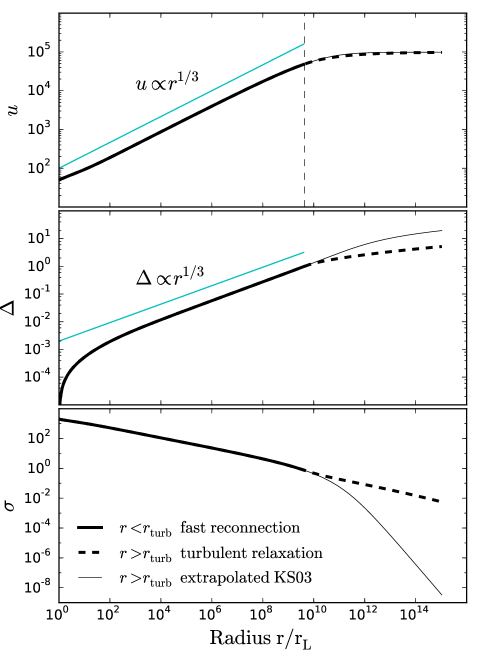
Figure 1.— Shown here is the four-velocity $u$ (top), and magnetization $\sigma$ (bottom) as a function of distance, for different models of a dissipative MHD wind with $\sigma_{0}=2000$. The thick solid curve is the “fast-reconnection” picture described in Kirk & Skjaraasen (2003). The vertical dashed line indicates the radius $r_{\rm turb}$ at which a dynamical time has elapsed in the comoving frame, and where the fast reconnection picture should break down. The dashed line shows evolution according to the turbulent relaxation picture.

Winds driven by obliquely rotating pulsars contain “stripes” around the equatorial region. The stripes are reversals of the azimuthal magnetic field, separated by a half-wavelength $\lambda=P_{\star}v/2$ (Michel, 1971, 1982). Magnetic reconnection across the reversals has been considered as a possible mechanism by which the wind’s electromagnetic energy may be dissipated upstream of the termination shock (Coroniti, 1990; Michel, 1994). However, those treatments neglected feedback of the dissipated magnetic energy on the global flow. Energy conserving analyses (Lyubarsky & Kirk, 2001; Kirk & Skjaraasen, 2003) revealed that dissipated magnetic energy goes toward accelerating the flow, due to reduction of inward-pointing magnetic hoop stress. As the flow moves faster, relativistic time dilation suppresses the dissipation rate as seen in the pulsar frame. The Crab Pulsar’s wind becomes weakly magnetized by the time it reaches the termination shock if it is at the upper end of believable mass-loading $\dot{N}\gtrsim 10^{40}\,\mathrm{s^{-1}}$.

The analysis given in Lyubarsky & Kirk (2001) was based on a plane-parallel reconnection model, in which cold, magnetized plasma fills the volume between hot, unmagnetized current layers. Hot current layers expand into the cold plasma at a speed $v_{\rm rec}$, consuming magnetic energy as they proceed. The fraction of volume occupied by hot plasma, denoted as $\Delta$, indicates how much of the initial magnetic energy has been consumed, $\zeta=(1-\Delta)\zeta_{0}$. To first order in both the expansion speed $v_{\rm rec}$ and the inverse Lorentz factor $\gamma^{-1}$, $\Delta$ evolves according to (see Appendix B)

$$\dot{\Delta}=2\frac{v_{\rm rec}}{\lambda\gamma}+\mathcal{O}(\gamma^{-2})+\mathcal{O}(v_{\rm rec}^{2})\,.$$ (14)

Thus, Lyubarsky’s prescription and ours are made equivalent by the identifications $\ell\rightarrow\lambda\gamma$, $v_{\rm rec}\rightarrow v_{A}/2$, and $\dot{\Delta}\rightarrow\tau^{-1}$, and by replacing $\zeta=(1-\Delta)\zeta_{0}$ with $\dot{\zeta}=-\dot{\Delta}\zeta$, so that $\Delta$ is formally allowed to exceed unity. Conveniently, $\Delta$ may here be interpreted as the number of elapsed Alfvén times felt by a fluid parcel.

It was argued in Zrake (2016) that the planar geometry of the current layers would only persist until order one comoving Alfvén times had elapsed, $\Delta\sim 1$. Subsequently the striped magnetic field becomes isotropic and dissipation should be described by turbulent relaxation. Thus, the onset of isotropic turbulence accompanies the transition to particle-dominated flow, which again, occurs upstream of the shock only if the wind is well mass-loaded. Nevertheless, we will explore briefly evolution of the striped wind, if it were allowed to expand freely beyond the turbulence transition. We do this by setting $\ell$ to $\lambda\gamma$ until $\Delta=1$, and henceforth evolving $\ell$ according to the turbulent relaxation model. For as long as $\Delta\ll 1$, $\sigma$ remains large and thus $v_{A}\approx c$. We expect the asymptotic solutions to obey the same scaling as the “fast reconnection” picture presented in Kirk & Skjaraasen (2003), because that also adopts constant reconnection speed (that of sound $c/\sqrt{3}$ in the hot plasma).

Figure 1 illustrates this equivalence for a hypothetical wind having a magnetization $\sigma_{0}=2000$, and which continues to $10^{15}r_{L}$ without passing through a termination shock. We see that indeed $\Delta$ and $u$ both evolve $\propto r^{1/3}$. Beyond $\Delta=1$, the solution is integrated in two ways: (1) by extending the fast reconnection picture, where $\ell$ remains equal to $\lambda\gamma$ and (2) by using the turbulent relaxation picture where $\ell$ increases according to Equation 13. Since roughly half of the magnetic energy has already been spent by the time $\Delta\sim 1$, further evolution of $u$ is not affected much by how dissipation is prescribed where $\Delta>1$. Magnetization $\sigma$, on the other hand, evolves much more slowly when turbulent growth of $\ell$ is accounted for.

3.2. Forced reconnection at the shock

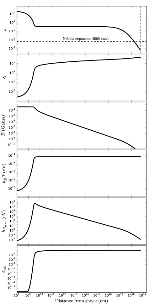
Figure 2.— Evolution of the post-shock pulsar striped wind. Shown here, from top to bottom, is the radial four-velocity $u$, cascade number $\Delta$, magnetic field strength $B$, electron temperature $k_{B}T$, photon energy $h\nu_{\rm sync}$, and radiated power $\varepsilon_{\rm rad}$, all as a function of distance downstream of the shock, for particular wind parameters $L_{\star}=5\times 10^{38}\,\mathrm{erg/s}$, $\dot{N}=10^{36}\,\mathrm{s^{-1}}$, and $\sigma_{0}=2\times 10^{5}$. Dissipation occurs in the “fast reconnection” regime upstream where $\Delta<1$, and in the turbulent regime once $\Delta\geq 1$. The horizontal dashed line in the top-most panel indicates the nominal nebula expansion speed $u_{\rm neb}=2000\,\mathrm{km/s}$, while the vertical dashed line marks the nominal nebula boundary $r_{\rm neb}=2\,\mathrm{pc}$.

Now we consider dissipation of the striped wind beyond the termination shock, assuming that it arrives there well magnetized. At the shock, the flow is compressed and decelerated below the fast magnetosonic speed. So, as discussed in Section 2.2, any dissipation that occurs beyond it only further decelerates the flow. Such “forced reconnection” has been studied in depth for its possible role in energizing at least some of the Crab Nebula’s radio-emitting, non-thermal electrons. However, as pointed out by Lyubarsky (2003b), the post-shock temperature is likely high enough that electron gyro-radii exceed the stripe wavelength, $r_{g}>\ell$. Electron heating in this regime has been studied using kinetic simulations by Lyubarsky & Liverts (2008). Forced reconnection of the striped wind has also been examined in a regime where post-shock kinetic scales remain smaller than the stripe separation, in both kinetic (Sironi & Spitkovsky, 2011) and hydromagnetic (Takamoto et al., 2012) settings. Here, we analyze the post-shock forced reconnection using our model, even though turbulent dissipation is probably not an appropriate treatment when the eddy scale is microscopic. Still, this approach extends the analysis of Lyubarsky (2003b), by resolving the forced reconnection zone. This approach also extends the analyses of Lyubarsky & Liverts (2008); Sironi & Spitkovsky (2011); Takamoto et al. (2012), which do resolve the post-shock reconnection zone, but do not account for the flow’s spherical geometry or its macroscopic evolution throughout the nebula. Our aim is to determine the magnetization and radiative efficiency of the nebular flow, at latitudes where stripes may be fully dissipated. This applies to the equatorial belt in the Crab Nebula, or at all latitudes in a hypothetical nebula powered by an orthogonally rotating pulsar.

We choose a set of wind parameters, $L_{\star}=5\times 10^{38}\,\mathrm{erg/s}$, $\dot{N}=10^{36}\,\mathrm{s^{-1}}$, and $\sigma_{0}=2\times 10^{5}$, intended to illustrate extreme electron heating and photon production in the forced reconnection. Such small mass-loading implies that the each particle must bear a relatively greater portion of the wind power, such that the post-shock temperature and thus synchrotron frequency is higher. The freely expanding wind is assumed to dissipate in the fast reconnection regime described in Section 3.1, because for these parameters, $\Delta$ remains small ($\lesssim 10^{-2}$) out to the shock. At the distance $r_{\rm ts}=3\times 10^{17}\,\mathrm{cm}$, we solve the Kennel-Coroniti jump conditions (see Equation C1) and continue integrating the solution on the downstream side of the shock. There, $\Delta^{\prime}$ increases dramatically such that $\Delta$ goes through unity after a few wavelengths $\sim 10^{9}-10^{10}\,\mathrm{cm}$. Once $\Delta>1$ we switch to the turbulent relaxation model.

A number of points are illustrated by the solution, shown in Figure 2. First, dissipation (and thus deceleration) occur rapidly on the downstream side of the shock, even though turbulent relaxation is slowed by the growth of $\ell$. Since we have assumed zero residual (stripe-averaged) magnetic field, reconnection proceeds toward arbitrarily small values of the magnetic field. This has two immediate consequences — (1) that the flow decelerates well below the nebula expansion velocity $u_{\rm neb}\approx 2000\,\mathrm{km/s}$, such that the outer boundary condition cannot be satisfied, and (2) that the magnetic field at large distance lies in the range of $10^{-9}\,\mathrm{G}$, much weaker than what is thought to exist in the Crab Nebula, $10^{-4}-10^{-3}\,\mathrm{G}$. Thus, orthogonal rotation of the Crab Pulsar is incompatible with our dissipation model. If a residual magnetic field is included , then only that part remains after a short distance beyond the shock. A residual field might well be interpreted as the magnetization invoked by Kennel & Coroniti (1984a) to match the nebula expansion. However, any such residual field at a given latitude should also be prone to reconnection by mixing across the nebula equator or succumbing to kink instabilities at high latitude. We analyze relaxation of the large-scale residual magnetic field in Section 4.

Figure 2 illustrates a number of points related to synchrotron radiation from the pulsar wind. First, effectively no radiation comes from the freely expanding wind; the synchrotron cooling time for streaming elections is vastly longer than their adiabatic cooling time. This point is already well appreciated, and known empirically from the Crab’s “underluminous” zone (e.g. Hester et al., 2002). Second, electrons are only heated up to $\sim 10^{10}\,\mathrm{eV}$ by the shock itself, but may be further heated (at least for the low mass-loading chosen here) up to $\sim 0.1\,\mathrm{PeV}$ in the forced reconnection immediately downstream. The associated photon energies reach to the MeV range. However, the magnetic field dissipates at short range to much lower values, and only $\sim 10^{-6}$ of the pulsar luminosity is ultimately converted into $\gamma$-rays.

The wind parameters chosen for this example are intentionally chosen to represent an extreme case of electron heating in the forced reconnection. For more realistic parameters, say $\dot{N}\sim 10^{38}$, the post-shock electron temperatures are typically in the TeV range, with associated photon energies in the UV to soft X-ray. However, the choice of wind parameters has little bearing on the profile of flow velocity and magnetic field strength at distances larger than $\sim 10^{17}\,\mathrm{cm}$. In particular, we have not identified any relevant wind parameters which yield a realistic radiative efficiency, again because the short-wavelength oscillating magnetic field dissipates too quickly; producing the high radiative efficiency inferred for the Crab requires a residual, or at least slowly dissipating component of the magnetic field. In the next section, we show that our turbulent relaxation model can match the outer boundary condition and radiative efficiency if applied to the large-scale toroidal magnetic field, rather than the striped wind.

4. Turbulent relaxation of the large-scale field in the Crab Nebula

We now turn to the question of how the large-scale toroidal magnetic field relaxes and dissipates in the volume of the nebula. This analysis intends to characterize the post-shock flow at moderate to high latitudes, where the oscillating magnetic field is small or zero. We thus evolve the freely expanding flow without any dissipation, while the post-shock flow is evolved using the turbulent relaxation prescription. We fix the wind luminosity $L_{\star}=5\times 10^{38}\,\mathrm{erg/s}$, which now stands for power supplied to the nebula in the form of non-oscillating magnetic field, and should thus, strictly speaking, be smaller by a factor of $\sim 3$ (Komissarov, 2012, assuming $45^{\circ}$ obliquity) than the pulsar spin-down power. The radiative efficiency is set to a nominal value of $\varepsilon_{\rm neb}=0.4$, which is marginally higher than current estimates in the range of $20-30\%$ (Hester, 2008). The eddy scale near the inner edge of the nebula, $\ell_{\rm sh}$ is left as a free parameter, to be determined by appropriate matching of the outer boundary condition. The corresponding rate $\tau_{\rm sh}^{-1}$ may be interpreted loosely as the growth rate of kink instabilities operating on the toroidal field around nebula’s X-ray core (Begelman, 1998). At larger distances the dissipation time-scale will increase. If the model is realistic, the volume average $\bar{\tau}$ will be close to $\sim 80\,\mathrm{yr}$, estimated by Komissarov (2012) from calorimetric considerations.

4.1. Numerical procedure

We identify a family of wind solutions, one for each value of $\ell_{\rm sh}$, that matches the nebula expansion speed $u_{\rm neb}=2000\,\mathrm{km/s}$ and radiative efficiency $\varepsilon_{\rm neb}=0.4$. We do this by numerically integrating 144 wind solutions, tabulated on an evenly spaced $12\times 12$ grid in $x\equiv\log\dot{N}$ and $y\equiv\log\sigma$. One such grid is generated for each of 30 different values of $\ell_{\rm sh}$. On each grid, [$u_{\rm neb}$, $\varepsilon_{\rm neb}$] is recorded at all lattice points $(x,y)$. We then prolong the grid by a factor of 8 in both variables using third-order splines. Next we construct a set of level surfaces $[x_{u,\varepsilon}(s)$, $y_{u,\varepsilon}(s)]$, parameterized in arc-length $s$, along which $u_{\rm neb}$, $\varepsilon_{\rm neb}$ take on constant values. Finally, we determine the intersection between the level surfaces by minimizing the distance function $\sqrt{[x_{u}(s_{u})-x_{\varepsilon}(s_{\varepsilon})]^{2}+[y_{u}(s_{u})-y_{\varepsilon}(s_{\varepsilon})]^{2}}$ over ($s_{u}$, $s_{\varepsilon}$). Figure 3 shows an example of one of the solution grids.

4.2. Results

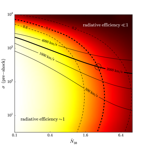
Figure 3.— Relief plot showing the radiative efficiency $\varepsilon_{\rm neb}$ of the post-shock flow in the Crab Nebula, as a function of the wind magnetization $\sigma$ and particle production rate $\dot{N}=10^{38}\dot{N}_{38}\,\mathrm{s^{-1}}$. The color indicates the fraction of pulsar spin-down power that has been converted into synchrotron photons once the flow reaches the nebula boundary at $\sim 2\,\mathrm{pc}$. Dashed contours are the level surfaces of radiative efficiency $\varepsilon_{\rm neb}$. The solid contours represent level surfaces of $u_{\rm neb}$, the nebula expansion speed at its boundary. The open circle at the intersection of the two heavier contours indicates the values of $\sigma$ and $\dot{N}$, that are favored by the turbulent relaxation model, given the fiducial values $\varepsilon_{\rm neb}=0.4$ and $u_{\rm neb}=2000\,\mathrm{km/s}$.

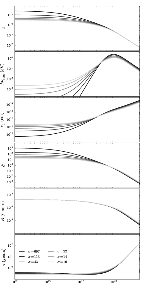
Figure 4.— Solutions of the post-shock nebular flow, when dissipation occurs due to large-scale turbulent processes. Shown are six solutions with upstream magnetizations $\sigma_{0}$ between 10 and 697, but that all satisfy the nebula boundary condition $u_{\rm neb}=2000\,\mathrm{km/s}$ and have a radiative efficiency $\varepsilon_{\rm neb}=0.4$. Shown, from top to bottom, is the four velocity $u$, photon energy $h\nu_{\rm sync}$, electron gyro-radius $r_{g}$, magnetization $\tilde{\sigma}\equiv\sigma/(1+\mu)$, magnetic field strength $B$, and local dissipation time-scale $\tau$, all as a function of distance downstream of the shock.

Exploration of the parameter space reveals that the outer boundary condition and the radiative efficiency can only be matched simultaneously when $\ell_{\rm sh}$ is quite near (within $\sim 30\%$ of) $r_{\rm ts}=3\times 10^{17}\,\mathrm{cm}$, and when $\dot{N}=10^{38}\,\mathrm{s^{-1}}$ to within a factor of $\sim 5$. On the other hand, the pre-shock value of $\sigma$ is found to be rather sensitive to $\ell_{\rm sh}$, ranging from $10$ when $\ell_{\rm sh}=2.8\times 10^{17}\,\mathrm{cm}$ to $697$ when $\ell_{\rm sh}=3.9\times 10^{17}\,\mathrm{cm}$. Figure 3 shows an example solution grid for which $\ell_{\rm sh}=3.5\times 10^{17}\,\mathrm{cm}$. The level surfaces of $u_{\rm neb}$ and $\varepsilon_{\rm neb}$ intersect at $\dot{N}=2.6\times 10^{38}\,\mathrm{s^{-1}}$ and $\sigma_{0}=285$. Radiative efficiency increases with lower mass-loading because each particle must bear a greater portion of the wind’s dissipated magnetic energy, and thus attains a higher thermal Lorentz factor. The nebula magnetic field strength is found to be relatively insensitive to $\dot{N}$.

Figure 4 shows six of the matching solutions for different values $\ell_{\rm sh}$, labeled for the value of $\sigma_{0}$ that satisfies the boundary conditions. The different solutions are largely distinguished by the post-shock speed, which for the higher magnetization value remains at $u\sim 10-20$ over $\sim 10^{16}-10^{17}\,\mathrm{cm}$ beyond the shock. For all solutions, the electron gyro-radius $r_{g}$ (and indeed the skin depth, not shown) is larger than the oscillating magnetic field wavelength, suggesting that any stripes would dissipate without energizing non-thermal electrons (Sironi & Spitkovsky, 2011). However, the kinetic scales remain everywhere much smaller than the eddy scale, indicating that MHD turbulent relaxation is an appropriate description of the mean field dissipation. Furthermore, non-thermal particle acceleration may be successful in the turbulent reconnection, since there the magnetic fluctuation scale is macroscopic.

Solutions are indistinguishable in the profile of magnetic field strength, which remains between 100 and $400\,\mathrm{\mu G}$ out to $10^{18}\,\mathrm{cm}$ and then declines to $10\,\mathrm{\mu G}$ by the nebula’s outer edge. The volume average of the nebula magnetic field is very nearly $60\,\mathrm{\mu G}$ in all our models, about half that required by the one-zone model of Meyer et al. (2010). The photon energy peaks at $10^{18}\,\mathrm{cm}$ in all models, and varies from $1-3\,\mathrm{eV}$ as $\sigma_{0}$ increases (and $\dot{N}$ decreases). The Crab spectrum peaks at around $4\,\mathrm{eV}$, so mass loadings at the lower end of our parameter range, $\dot{N}_{38}=2.5$, are weakly favored. Electron temperatures are from $100-200\,\mathrm{GeV}$ around $r=10^{18}\,\mathrm{cm}$, and the gyro-radii are from $10^{13}-10^{14}\,\mathrm{cm}$. Meanwhile, the turbulent eddy scale (not shown in the figure) increases from $\sim r_{\rm ts}$ by a factor of roughly 10, to $\sim r_{\rm neb}$ at the outer edge, so the relaxation picture becomes marginally inapplicable there. The dissipation time-scale varies from about 4 months near the nebula core, to over 100 years at the outer edge. The volume average is $\bar{\tau}\approx 52$ years for all models, slightly lower than the 80-year dissipation time scale determined in Komissarov (2012).

5. Discussion and conclusions

We have developed a model for turbulent magnetic reconnection in a pulsar wind nebula. The model is based on stationary, one-dimensional MHD flow which embeds a freely relaxing, small-scale magnetic field. Such characterization of the internal magnetic field allows for a dissipation model that is supported by recent developments in the theory of relativistic magnetic reconnection and turbulent relaxation. We examined separately dissipation of the striped wind in both the freely expanding and post-shock flow, as well as turbulent relaxation of the mean magnetic field beyond the termination shock. Applied to the Crab Nebula, this model reproduces the expansion speed, radiative efficiency, and peak photon frequency within a one-parameter family of solutions, and without invoking unrealistically low values of the upstream magnetization, as required in the historical non-dissipative models. Our model strongly favors a pulsar particle production rate $\dot{N}=2.5\times 10^{38}\,\mathrm{s^{-1}}$, and a magnetic thermalization time scale which evolves from roughly 4 months (the light-travel time of the wind termination shock radius) near the nebula core, to 100 years near its outer edge. Such slowing of the turbulent cascade rate with distance is not put in by hand, but results from scaling laws derived from three-dimensional numerical simulations of turbulent magnetic relaxation (Zrake, 2014). We have also introduced a simple formalism for incorporating optically thin synchrotron losses into steady-state MHD winds. Though not critical in the dynamics of the Crab Pulsar wind, we will point out in Section 5.4 that the radiative losses may dominate the reverse shock dynamics in the striped wind of a “millisecond magnetar”.

5.1. Limitations

The model we have developed here is overly simplistic in a number of ways. First, we do not account for any non-spherical geometry. In this approximation, the equations of motion and the shock jump conditions are formally valid in transverse MHD only at the equator. More realistic, two-dimensional shock jump conditions have been analyzed in connection with the Crab’s inner knot feature (Yuan & Blandford, 2015; Lyutikov et al., 2016a). Also, in treating the radiative losses we assumed that particles were mono-energetic, whereas Kennel & Coroniti (1984b) produced integrated spectra by assuming that particles occupy a power-law in energy. In principle, we could have done the same here, but that would require a particle spectral index to be selected by hand. Given that the magnetic field strength and coherence scale are both predicted by the model, the particle spectrum could be truncated at the energy where gyro-radii would exceed the local eddy scale. A more sophisticated treatment along these lines may be pursued in a future work.

5.2. Crab $\gamma$-ray flares

The Crab’s $\gamma$-ray flares (Tavani et al., 2011; Abdo et al., 2011) have been widely interpreted as the signature of exceptionally powerful reconnection episodes (Uzdensky et al., 2011; Clausen-Brown & Lyutikov, 2012; Cerutti et al., 2012, 2014a, 2014b; Nalewajko et al., 2016; Yuan et al., 2016; Lyutikov et al., 2016b). Reconnection is most promising to explain flares if it occurs where the plasma is strongly magnetized. As pointed out by Lyubarsky (2012), such a region is expected to occur in the $z$-pinch at high latitudes. In his model, the core of the pinch would be of the order $10^{16}\,\mathrm{cm}$, roughly the scale of the emitting region as implied by the $\sim 10\,\mathrm{hr}$ flare duration. Despite the rather artificial geometry of our own model, it also predicts a strongly magnetized region region, $\tilde{\sigma}\lesssim 10^{3}$ of scale $10^{16}-10^{17}\,\mathrm{cm}$, when the upstream magnetization is high. Interestingly, in that region (just past the termination shock, see Figure 4) plasma moves radially outward with a Lorentz factor $\lesssim 20$. The implied Doppler beaming could help account for the spectral cutoff, which for some flares exceeds the radiation reaction limit $\sim 100\,\mathrm{MeV}$ (e.g. Buehler et al., 2012). In our model, the post-shock flow is relativistic and strongly magnetized only where stripes are negligible. Where they dominate, the magnetization decreases and the flow decelerates immediately beyond the shock in the forced reconnection (see Figure 2). This may still be consistent with a scenario discussed in Arons (2002), where the flaring region lies marginally upstream (or perhaps within the kinetic structure) of the termination shock, where the radial Lorentz factor remains high.

5.3. Evolution of the PWN particle spectrum

We hope that the model developed here will find utility in multi-zone modeling of particle transport and acceleration in PWNe. This could be useful in modeling of PWNe for which multi-band, spatially resolved observations are available, such as MSH 15-52 (e.g. An et al., 2014) and 3C 58, not to mention the Crab. It could also help determine the rate of positron leakage from the nebula, and help assess the importance of PWNe as galactic positron sources. Unlike one-zone models (Gelfand et al., 2009; Bucciantini et al., 2011) for which the spectral energy distribution of injected electrons is a model parameter, a multi-zone treatment could possibly predict the spectrum from humbler assumptions. For example, one might solve an advection-diffusion equation, where the advective part is given by the flow velocity $u$, and the spatial diffusion by the eddy scale $\ell$ and fluctuating velocity $v_{A}$. The latter yields a turbulent diffusivity, while the local specific heating rate $\dot{\zeta}$ may be used to normalize energy gains by the electron population. This may be taken up in a future work.

5.4. EM counterparts from “millisecond magnetars”

Rapidly rotating, strongly magnetized neutron stars have been invoked in connection with a variety of observed and hypothetical astrophysical transients. Many $\gamma$-ray bursts, both long and short, exhibit an extended X-ray emission plateau, which has been widely interpreted as the signature of sustained energy injection by a nascent PWN. Generally, one imagines the nebula to be confined by a massive shell, either of stellar ejecta in the case of long bursts and superluminous supernovae, or material dynamically expelled from a binary neutron star merger in the case of short bursts. In either scenario, the resulting emission is expected to be more isotropic than the $\gamma$-ray burst itself, and is thus interesting as a possible electromagnetic counterpart to gravitational wave detections of binary neutron star coalescence.

Conditions in these hypothetical PWNe are qualitatively distinct in a couple of ways from those of the Crab Nebula. The radiative energy density $\varepsilon_{\rm rad}$ in the nascent nebula could be so high as to initiate a cascade of $e^{\pm}$ pair production, so that mass conservation $df=0$ does not apply. As a result, the plasma density may be high enough to trap synchrotron photons, so that $d\eta=0$ even when $P_{\rm sync}\neq 0$. Pair production is robust when the nebula compactness parameter

$$\ell_{c}=(\varepsilon_{\rm rad}/m_{e}c^{2})\,\sigma_{T}\,\delta R_{\rm neb}$$ (15)

is high. As we saw in Section 3.2 the pre-shock flow is cold and non-radiative, so pair production should only commence in the region of width $\delta R_{\rm neb}$ between the reverse shock and the confining shell. Equation 15 indicates that if some photons were to leak out from the nebula, then pair production would be suppressed for two reasons. The first, of course, is that leakage reduces $\varepsilon_{\rm rad}$ and thus $\ell_{c}$ directly. The second is that loss of radiation pressure in the shocked plasma allows the reverse shock to advance toward the shell, reducing $\delta R_{\rm neb}$. This further decreases the nebula optical depth, meaning that a slightly “deflated” nebula only becomes more leaky.

Of course, the details of radiation leakage from nascent PWNe are beyond the present scope. Nevertheless, we make two observations here that could motivate future more detailed calculations. First, we point out that under conditions relevant to binary neutron star mergers (those yielding a millisecond magnetar), the synchrotron efficiency of the reverse shock can go up to $100\%$, with all the radiation produced above $100\,\mathrm{MeV}$. Photon losses may become relevant at such high energies because Klein-Nishina effects reduce the optical depth of the shocked plasma and confining shell. Also, the relevant shell albedo would be that of $\gamma$-rays, while X-ray albedo has been adopted in earlier analyses (Metzger et al., 2013; Metzger & Piro, 2014; Kasen et al., 2016). Second, we argue that the pair cascade might in some cases appear intermittently or not at all.

Consider the special case of a stable millisecond magnetar formed in a binary neutron star merger. We adopt nominal source parameters $L=5\times 10^{47}\,\mathrm{erg/s}$, $\dot{N}=10^{48}\,\mathrm{s^{-1}}$, and $\sigma_{0}=5\times 10^{3}$, and place the ejecta at $R_{\rm ej}=0.1c\times 1\,\mathrm{hr}\approx 10^{13}\,\mathrm{cm}$, moving outwards at $0.1c\approx 30,000\,\mathrm{km/s}$. Now suppose the pulsar is an orthogonal rotator, so that its electromagnetic power is all in the striped wind as we analyzed in Section 3. With those parameters fixed, vary the shock location until the flow matches smoothly onto the ejecta. If the plasma is optically thick, then synchrotron losses should be ignored as photons are trapped and contribute to the gas pressure with the same equation of state, $\Gamma=4/3$ as the plasma particles. In this case, the shock is found to lie about half way to the ejecta shell (similar to Figure 2), so the assumption $\delta R_{\rm neb}\sim R_{\rm ej}$ in calculating $\ell_{c}$ (e.g. Metzger et al., 2013) appears to be well justified. However, unlike the result shown in Figure 2 for Crab parameters, the synchrotron frequency is $\gtrsim 100\,\mathrm{MeV}$, and the efficiency $\varepsilon_{\rm rad}$ in the forced reconnection zone is essentially 100%. Accounting for the Klein-Nishina suppression, $\kappa\approx 10^{-2}$ at $100\,\mathrm{MeV}$,

$$\tau_{\rm neb}=\kappa\,\sigma_{T}\,n_{e}\,\delta R_{\rm neb}\vspace{1 mm}$$

is found to be $\lesssim 10^{-2}$. Therefore, synchrotron photons produced at the reverse shock traverse the nebula, and their fate is determined by the albedo and optical depth of the shell. If insufficient radiation were reflected back to the nebula, then $\varepsilon_{\rm rad}$ and thus $\ell_{c}$ would be small, and the pair cascade could fail.

Of course, the preceding analysis ignores the enhancement of $n_{e}$ brought on by a pair cascade. If one operates, then once again $\tau_{\rm neb}\gg 1$, photons are trapped, radiation pressure forces the reverse shock to recede inwards, the compactness parameter is kept large, and pair production continues. But this illustrates the point made previously, that the pair cascade depends on itself to survive, and is thus a complex problem. Unraveling the non-linear physics may require a detailed calculation of fully coupled magnetic reconnection, synchrotron radiation, photon propagation, and pair production processes. It is difficult to say whether such a pursuit would be fruitful in the present context. Nevertheless, similarly complex relativistic plasma systems were examined by Timokhin & Arons (2013), and also by Beloborodov (2016) with interesting applications to pulsars and $\gamma$-ray burst prompt emission, respectively. Continued research along these lines was advocated for by Uzdensky (2015).

Appendix A Turbulent relaxation model

Coherent magnetic structures (eddies, or flux tubes) grow over time by merging with one another as a result of coalescence instability (e.g. Finn & Kaw, 1977; East et al., 2015), and they also grow or shrink due to the expansion or compression of comoving volume. For the latter reason it is convenient to utilize the eddy mass $m$ as a proxy for its scale. In three dimensions, magnetic structures are cylindrical flux tubes, having mass $m\sim\rho\ell^{3}$ (assuming their length and radius are comparable). The flux tubes are locally relaxed equilibria and thus generally helical (Matthaeus & Montgomery, 1980; Matthaeus et al., 2012), having comparable axial and azimuthal field strength. When net magnetic helicity is zero, left and right polarized flux tubes exist in equal number. Pairs can join by reconnecting their azimuthal field when their axial electric current vectors are parallel, but they only form a stable structure when their axial magnetic fields are also parallel; otherwise the axial field annihilates and renders the merged flux tube kink-unstable. Thus only half of the merging episodes (those occurring between like-polarized tubes) yield stable structures, and so the total number of eddies $s$ decreases by a factor of four in each stage of coalescence, $s_{n+1}=s_{n}/4$. Stages proceed at the cascade rate

$$\dot{n}=\frac{v_{\rm rec}}{\ell}\,,$$

where $v_{\rm rec}$ is given roughly by the local Alfvén speed $v_{A}=(\sigma/w)^{1/2}$. Each merging event conserves mass and magnetic helicity, so we have $m_{n+1}=2m_{n}$ and $h_{n+1}=2h_{n}$. Meanwhile, the magnetic energy per eddy drops according to $\epsilon_{n}=h_{n}/\ell_{n}$. The volume-averaged magnetic energy per unit mass is given by $\sigma_{n}=s_{n}\epsilon_{n}/\rho$. Here, the cascade number $n$ is a discrete version of the variable $\Delta$ used throughout the paper.

When expansion is neglected ($\dot{\rho}=0$), this heuristic yields a decay law in which the characteristic eddy scale increases over time as $\ell\propto t^{2/5}$, and the magnetic energy decays as $\sigma\propto t^{-6/5}$. Such behavior was seen by Zrake (2014) in simulations of freely decaying, non-helical relativistic MHD turbulence in three dimensions. However, the heuristic’s applicability to an expanding volume has not yet been explored directly with numerical simulations. Arguably, one expects the eddy mass to be a good proxy for its scale whenever the turbulence cascade rate $\dot{n}$ is fast compared with the secular evolution. Comoving volume in the pulsar wind expands at a rate $\omega_{\perp}=u/r$ in the transverse direction, and at $\omega_{\parallel}=\dot{u}/u$ in the longitudinal direction. If either of the expansion rates was faster than $\dot{n}$, the magnetic field pattern would become frozen into the flow, and get stretched in whichever direction expands faster. This situation corresponds to the magnetic free energy scale exceeding that of the local horizon. Provided the cascade is faster than both expansion rates, eddies maintain their isotropy in the comoving frame, and use of the mass coordinate in place of scale is well justified.

Appendix B Plane-parallel reconnection picture

Here we review the conditions under which the plane-parallel reconnection picture of Lyubarsky & Kirk (2001) is equivalent to the turbulent relaxation model. Near the pulsar, the striped wind consists of cold, well-magnetized plasma. The azimuthal magnetic field alternates in direction every half-wavelength $\lambda=P_{\star}v/2$. Magnetic reconnection operates around the reversals, causing slabs of hot plasma to expand at a speed $v_{\rm rec}$. The hot regions occupy a fraction $\Delta$ of the wind volume, and so $1-\Delta$ is the surviving fraction of the wind’s magnetic energy. Consider a cold plasma volume which is bounded by current layers centered at $r_{1},r_{2}$. As the current layers expand, the one centered at $r_{1}$ extends forward to $r_{+}$, while the one centered at $r_{2}$ extends backward to $r_{-}$, so we have

$$\Delta=1-\frac{r_{-}-r_{+}}{r_{2}-r_{1}}\,.$$ (B1)

Now, $\frac{dr_{1}}{dt}=v$ and to linear order $\frac{dr_{2}}{dt}=v+\lambda\frac{dv}{dr}$, where $\lambda=r_{2}-r_{1}$ and $t$ here denotes time in the pulsar frame. The velocity gradient is given by $\frac{dv}{dr}=\omega_{\parallel}\gamma^{-3}$ where $\omega_{\parallel}=\dot{u}/u=\frac{du}{dr}$ is the acceleration rate. The reconnection fronts advance according to the relativistic velocity addition of the flow and $v_{\rm rec}$,

$$\frac{d}{dt}r_{\pm}=\frac{v_{\pm}\pm v_{\rm rec}}{1+v_{\pm}v_{\rm rec}}\,,$$ (B2)

where $v_{\pm}=v+(r_{\pm}-r_{1})\frac{dv}{dr}$. We also assume that $r_{1}+r_{2}=r_{-}+r_{+}$. Since the wind is ultra-relativistic, we expand $\dot{\Delta}=\gamma\frac{d\Delta}{dt}$ in powers of $\gamma^{-1}$,

$$\dot{\Delta}=\frac{2v_{\rm rec}}{1-v_{\rm rec}^{2}}\left\{\frac{1}{\lambda}\gamma^{-1}-\omega_{\parallel}\left[1+v_{\rm rec}(1-\Delta)\right]\gamma^{-2}+\mathcal{O}(\gamma^{-3})\right\}\,.$$ (B3)

Further dropping terms of order higher than $v_{\rm rec}^{2}$, we arrive at

$$\dot{\Delta}=\frac{2v_{\rm rec}}{\lambda\gamma}+\mathcal{O}(v_{\rm rec}^{2})+\mathcal{O}(\gamma^{-2})\,,$$

which is the same as Equation 14, and equivalent to Equation C3 of Kirk & Skjaraasen (2003). The second order term in Equation B3 inhibits the progress of reconnection fronts by stretching the background flow, but remains small provided $\lambda\gg h_{\rm rec}$, where $h_{\rm rec}=u_{\rm rec}/\omega_{\parallel}$ is the local horizon scale with respect to the reconnection speed. Sticking to first order in $\gamma^{-1}$ is thus sufficiently accurate unless reconnection were somehow to proceed ultra-relativistically.

Appendix C Shock jump conditions

The Kennel-Coroniti jump conditions are given by conservation of mass, magnetic flux, energy, and momentum across the shock,

$$u_{1}\rho_{1} = u_{2}\rho_{2}$$

$$u_{1}\sigma_{1} = u_{2}\sigma_{2}$$

$$\gamma_{1}w_{1} = \gamma_{2}w_{2}$$

$$u_{1}w_{1}+\frac{1}{u_{1}}\left(\frac{p_{1}}{\rho_{1}}+\frac{\sigma_{1}}{2}\right) = u_{2}w_{2}+\frac{1}{u_{2}}\left(\frac{p_{2}}{\rho_{2}}+\frac{\sigma_{2}}{2}\right)\,,$$

where subscripts 1 and 2 refer to values just ahead of, and just behind the shock respectively. Together with the $\Gamma$-law equation of state, these yield the following equation for the density jump $\delta\equiv\rho_{1}/\rho_{2}$ across the shock,

$$\eta\left(\delta\frac{1+\frac{\Gamma}{\Gamma-1}u_{1}^{2}}{\sqrt{1+u_{1}^{2}}}-\frac{1+\frac{\Gamma}{\Gamma-1}u_{1}^{2}\delta^{2}}{\sqrt{1+u_{1}^{2}\delta^{2}}}\right)-\sigma_{1}\left(\frac{\Gamma-2}{\Gamma-1}\right)\left(\frac{\delta^{2}-1}{2\delta}\right)=\delta-1\,.$$ (C1)

References

- Abdo et al. (2011) Abdo, A. A., Ackermann, M., Ajello, M., et al. 2011, Science (New York, N.Y.), 331, 739
- An et al. (2014) An, H., Madsen, K. K., Reynolds, S. P., et al. 2014, The Astrophysical Journal, 793, 90
- Arnold (1965) Arnold, V. 1965, Comptes Rendus Hebdomadaires des Seances de L’Academie des Sciences, 261, 17
- Arons (2002) Arons, J. 2002, The Astrophysical Journal, Volume 589, Issue 2, pp. 871-892., 589, 871
- Begelman (1998) Begelman, M. C. 1998, The Astrophysical Journal, 493, 291
- Begelman & Li (1992) Begelman, M. C., & Li, Z.-Y. 1992, The Astrophysical Journal, 397, 187
- Begelman & Li (1994) —. 1994, The Astrophysical Journal, 426, 269
- Beloborodov (2016) Beloborodov, A. M. 2016, eprint arXiv:1604.02794, arXiv:1604.02794
- Brandenburg et al. (2015) Brandenburg, A., Kahniashvili, T., & Tevzadze, A. G. 2015, Physical Review Letters, 114, 075001
- Bucciantini et al. (2011) Bucciantini, N., Arons, J., & Amato, E. 2011, Monthly Notices of the Royal Astronomical Society, 410, 381
- Buehler et al. (2012) Buehler, R., Scargle, J. D., Blandford, R. D., et al. 2012, The Astrophysical Journal, 749, 26
- Campanelli (2016) Campanelli, L. 2016, The European Physical Journal C, 76, 1
- Cerutti et al. (2012) Cerutti, B., Werner, G. R., Uzdensky, D. A., & Begelman, M. C. 2012, The Astrophysical Journal, 754, L33
- Cerutti et al. (2014a) —. 2014a, Physics of Plasmas, 21, 056501
- Cerutti et al. (2014b) —. 2014b, The Astrophysical Journal, 782, 104
- Chi et al. (1996) Chi, X., Cheng, K. S., & Young, E. C. M. 1996, The Astrophysical Journal, 459, L83
- Chiueh et al. (1991) Chiueh, T., Li, Z.-Y., & Begelman, M. C. 1991, The Astrophysical Journal, 377, 462
- Clausen-Brown & Lyutikov (2012) Clausen-Brown, E., & Lyutikov, M. 2012, Monthly Notices of the Royal Astronomical Society, 426, 1374
- Coroniti (1990) Coroniti, F. V. 1990, The Astrophysical Journal, 349, 538
- Dessart et al. (2012) Dessart, L., Hillier, D. J., Waldman, R., Livne, E., & Blondin, S. 2012, Monthly Notices of the Royal Astronomical Society: Letters, 426, L76
- Drenkhahn (2002) Drenkhahn, G. 2002, Astronomy and Astrophysics, 387, 714
- East et al. (2015) East, W. E., Zrake, J., Yuan, Y., & Blandford, R. D. 2015, Physical Review Letters, 115, 095002
- Finn & Kaw (1977) Finn, J. M., & Kaw, P. K. 1977, Physics of Fluids, 20, 72
- Frisch et al. (1975) Frisch, U., Pouquet, A., Leorat, J., & Mazure, A. 1975, Journal of Fluid Mechanics, 68, 769
- Gao et al. (2013) Gao, H., Ding, X., Wu, X.-F., Zhang, B., & Dai, Z.-G. 2013, The Astrophysical Journal, 771, 86
- Gelfand et al. (2009) Gelfand, J. D., Slane, P. O., & Zhang, W. 2009, The Astrophysical Journal, 703, 2051
- Giannios & Spruit (2007) Giannios, D., & Spruit, H. C. 2007, Astronomy and Astrophysics, 469, 1
- Goldreich & Julian (1969) Goldreich, P., & Julian, W. H. 1969, The Astrophysical Journal, 157, 869
- Goldreich & Julian (1970) —. 1970, The Astrophysical Journal, 160, 971
- Harding et al. (2008) Harding, A. K., Stern, J. V., Dyks, J., & Frackowiak, M. 2008, The Astrophysical Journal, 680, 1378
- Hester (2008) Hester, J. J. 2008, Annual Review of Astronomy and Astrophysics, 46, 127
- Hester et al. (2002) Hester, J. J., Mori, K., Burrows, D., et al. 2002, The Astrophysical Journal, 577, L49
- Kasen & Bildsten (2010) Kasen, D., & Bildsten, L. 2010, The Astrophysical Journal, 717, 245
- Kasen et al. (2016) Kasen, D., Metzger, B. D., & Bildsten, L. 2016, The Astrophysical Journal, 821, 36
- Kennel & Coroniti (1984a) Kennel, C. F., & Coroniti, F. V. 1984a, The Astrophysical Journal, 283, 694
- Kennel & Coroniti (1984b) —. 1984b, The Astrophysical Journal, 283, 710
- Kennel et al. (1983) Kennel, C. F., Fujimura, F. S., & Okamoto, I. 1983, Geophysical and Astrophysical Fluid Dynamics, 26
- Kirk & Skjaraasen (2003) Kirk, J. G., & Skjaraasen, O. 2003, The Astrophysical Journal, 591, 366
- Komissarov (2012) Komissarov, S. S. 2012, Monthly Notices of the Royal Astronomical Society, 428, 2459
- Liu et al. (2016) Liu, L. D., Wang, L. J., & Dai, Z. G. 2016, Astronomy & Astrophysics, 592, A92
- Lyubarsky & Kirk (2001) Lyubarsky, Y., & Kirk, J. G. 2001, The Astrophysical Journal, 547, 437
- Lyubarsky & Liverts (2008) Lyubarsky, Y., & Liverts, M. 2008, The Astrophysical Journal, 682, 1436
- Lyubarsky (2002) Lyubarsky, Y. E. 2002, Monthly Notices of the Royal Astronomical Society, 329, L34
- Lyubarsky (2003a) —. 2003a, Monthly Notices of the Royal Astronomical Society, 339, 765
- Lyubarsky (2003b) —. 2003b, Monthly Notices of the Royal Astronomical Society, 345, 153
- Lyubarsky (2012) —. 2012, Monthly Notices of the Royal Astronomical Society, 427, 1497
- Lyutikov et al. (2016a) Lyutikov, M., Komissarov, S. S., & Porth, O. 2016a, Monthly Notices of the Royal Astronomical Society, 456, 286
- Lyutikov et al. (2016b) Lyutikov, M., Sironi, L., Komissarov, S., & Porth, O. 2016b, arXiv:1603.05731
- Matthaeus & Montgomery (1980) Matthaeus, W. H., & Montgomery, D. 1980, Annals of the New York Academy of Sciences, 357, 203
- Matthaeus et al. (2012) Matthaeus, W. H., Montgomery, D. C., Wan, M., & Servidio, S. 2012, Journal of Turbulence, 13, N37
- Metzger et al. (2011) Metzger, B. D., Giannios, D., Thompson, T. A., Bucciantini, N., & Quataert, E. 2011, Monthly Notices of the Royal Astronomical Society, 413, 2031
- Metzger & Piro (2014) Metzger, B. D., & Piro, A. L. 2014, Monthly Notices of the Royal Astronomical Society, Volume 439, Issue 4, p.3916-3930, 439, 3916
- Metzger et al. (2013) Metzger, B. D., Vurm, I., Hascoet, R., & Beloborodov, A. M. 2013, Monthly Notices of the Royal Astronomical Society, Volume 437, Issue 1, p.703-720, 437, 703
- Meyer et al. (2010) Meyer, M., Horns, D., & Zechlin, H.-S. 2010, Astronomy & Astrophysics, 523, A2
- Michel (1969) Michel, F. C. 1969, The Astrophysical Journal, 158, 727
- Michel (1971) —. 1971, Comments on Astrophysics and Space Physics, 3
- Michel (1982) —. 1982, Reviews of Modern Physics, 54, 1
- Michel (1994) —. 1994, The Astrophysical Journal, 431, 397
- Mignone et al. (2013) Mignone, A., Striani, E., Tavani, M., & Ferrari, A. 2013, Monthly Notices of the Royal Astronomical Society, Volume 436, Issue 2, p.1102-1115, 436, 1102
- Mizuno et al. (2011) Mizuno, Y., Lyubarsky, Y., Nishikawa, K.-I., & Hardee, P. E. 2011, The Astrophysical Journal, 728, 90
- Nalewajko et al. (2016) Nalewajko, K., Zrake, J., Yuan, Y., East, W., & Blandford, R. 2016, Astrophysical Journal, 826, doi:10.3847/0004-637X/826/2/115
- Porth et al. (2013a) Porth, O., Komissarov, S. S., & Keppens, R. 2013a, Monthly Notices of the Royal Astronomical Society: Letters, 431, L48
- Porth et al. (2013b) —. 2013b, Monthly Notices of the Royal Astronomical Society, 438, 278
- Rees & Gunn (1974) Rees, M. J., & Gunn, J. E. 1974, Monthly Notices of the Royal Astronomical Society, 167, 1
- Rybicki & Lightman (1979) Rybicki, G. B., & Lightman, A. P. 1979, New York
- Sironi & Spitkovsky (2011) Sironi, L., & Spitkovsky, A. 2011, The Astrophysical Journal, 741, 39
- Takamoto et al. (2012) Takamoto, M., Inoue, T., & Inutsuka, S.-i. 2012, The Astrophysical Journal, 755, 76
- Tavani et al. (2011) Tavani, M., Bulgarelli, A., Vittorini, V., et al. 2011, Science (New York, N.Y.), 331, 736
- Taylor (1974) Taylor, J. B. 1974, Physical Review Letters, 33, 1139
- Timokhin & Arons (2013) Timokhin, A. N., & Arons, J. 2013, Monthly Notices of the Royal Astronomical Society, 429, 20
- Uzdensky (2015) Uzdensky, D. A. 2015, Magnetic Reconnection, Astrophysics and Space Science Library, Volume 427. ISBN 978-3-319-26430-1. Springer International Publishing Switzerland, 2016, p. 473, 427, 473
- Uzdensky et al. (2011) Uzdensky, D. A., Cerutti, B., & Begelman, M. C. 2011, The Astrophysical Journal, 737, L40
- Woosley (2010) Woosley, S. E. 2010, The Astrophysical Journal Letters, 719, L204
- Yuan & Blandford (2015) Yuan, Y., & Blandford, R. 2015, Monthly Notices of the Royal Astronomical Society, Volume 454, Issue 3, p.2754-2769, 454, 2754
- Yuan et al. (2016) Yuan, Y., Nalewajko, K., Zrake, J., East, W. E., & Blandford, R. D. 2016, The Astrophysical Journal, 828, 92
- Zhang (2013) Zhang, B. 2013, The Astrophysical Journal Letters, 763, L22
- Zrake (2014) Zrake, J. 2014, The Astrophysical Journal, 794, L26
- Zrake (2016) —. 2016, The Astrophysical Journal, 823, 39
- Zrake & East (2016) Zrake, J., & East, W. E. 2016, The Astrophysical Journal, 817, 89
- Zrake & MacFadyen (2013) Zrake, J., & MacFadyen, A. I. 2013, The Astrophysical Journal, 769, L29