Radiative corrections to elastic proton-electron scattering measured in coincidence

Abstract

The differential cross section for elastic scattering of protons on electrons at rest is calculated taking into account the QED radiative corrections to the leptonic part of interaction. These model-independent radiative corrections arise due to emission of the virtual and real soft and hard photons as well as to vacuum polarization. We analyze an experimental setup when both the final particles are recorded in coincidence and their energies are determined within some uncertainties. The kinematics, the cross section, and the radiative corrections are calculated and numerical results are presented.

I Introduction

The polarized and unpolarized scattering of electrons off protons has been widely studied, as it is considered the simpler way to access information on the proton structure, assuming that the interaction occurs through the exchange of a virtual photon of four-momentum $q$. The experimental determination of the elastic proton electromagnetic form factors in the region of small and large momentum transfer squared is one of the major field of research in hadron physics (see the review Pacetti et al. (2015)). New experimental possibilities allowed to reach better precision and to perform polarization experiments as earlier suggested in Refs. Akhiezer and Rekalo (1968, 1974).

The determination of the proton electromagnetic form factors, at $Q^{2}=-q^{2}\geq 1$ GeV², from polarization observables showed a surprising result: the polarized and unpolarized experiments, although based on the same theoretical background (same formalism and same assumptions), ended up with inconsistent values of the form factor ratio (see Puckett et al. (2010) and references therein). Possible explanation of this discrepancy is to take into account higher order radiative corrections Kuraev et al. (2014); Gramolin and Nikolenko (2016) including the interference between one and two photon exchange Arrington (2004), correlations among parameters Tomasi-Gustafsson (2007), normalization of data Pacetti and Gustafsson (2016). This puzzle has given rise to many speculations and different interpretations, suggesting further experiments (for a review, see Ref. Perdrisat et al. (2007)).

In the region of small $Q^{2}$ one can determine the proton charge radius ($r_{E}$) which is one of the fundamental quantities in physics. Precise knowledge of its value is important for the understanding of the structure of the nucleon in the theory of strong interactions (QCD) as well as in the spectroscopy of atomic hydrogen.

Recently, the determination of the $r_{E}$ with muonic atoms lead to the so-called proton radius puzzle. Experiments on muonic hydrogen by laser spectroscopy measurement of the $\mu$p (2S-2P) transition frequency, in particular the latest result on the proton charge radius Pohl et al. (2010); Antognini et al. (2013) $r_{E}=0.84087(39)$ fm, is one order of magnitude more precise but smaller by seven standard deviations compared to the average value $r_{E}=0.8775(51)$ fm which is recommended by the 2010-CODATA review Mohr et al. (2016). The CODATA value is obtained coherently from hydrogen atom spectroscopy and electron-proton elastic scattering measurements. The latest experiments with electrons at Jlab Zhan et al. (2011) and MAMI Bernauer et al. (2010) confirm this value, and, therefore, do not agree with the results on the proton radius from of the laser spectroscopy of the muonic hydrogen.

While the corrections to the laser spectroscopy experiments seem well under control in the frame of QED and may be estimated with a precision better than 0.1%, in case of electron-proton elastic scattering the best achieved precision is of the order of few percent. Different sources of possible systematic errors of the muonic experiment have been discussed, however no definite explanation of this difference has been given yet (see Ref. Antognini et al. (2011) and references therein).

The proton radius puzzle lead to a large number of theoretical papers suggesting solutions based on different approaches, as new physics beyond the Standard Model Tucker-Smith and Yavin (2011); Batell et al. (2011). Other approaches analyze the extraction of the proton radius from the electron-proton scattering data. In Ref. Giannini and Santopinto (2013), it is argued that a proper Lorentz transformation of the form factors accounts for the discrepancy. The authors of Ref. Kraus et al. (2014) stated that radius extraction with Taylor series expansions cannot be trusted to be reliable. A fit function based on a conformal mapping was used in Ref. Lorenz et al. (2012, 2015). The extracted value of the proton radius agrees with the one obtained from muonic hydrogen. A similar result was obtained in Ref.Horbatsch et al. (2016) using the approach based on the chiral perturbation theory Peset and Pineda (2014).

In Ref. Griffioen et al. (2016), the authors argued that the proton radius puzzle can be explained by truncating the electron scattering data to low momentum transfer. But the authors of Ref. Distler et al. (2015) showed that the procedure is inconsistent and violates the Fourier theorem. The authors of the paper Bernauer and Distler (2016) inspected several recent refits of the Mainz data, that result in small radii and found flaws of various kinds in all of them.

A recent review summarizes the current state of the problem and gives an overview over upcoming experiments Bernauer (2014).

More experiments in the region of small $Q^{2}$ are expected to shed some light on this intriguing problem. The PRad collaboration Gasparian (2014) is currently preparing a new magnetic-spectrometer-free electron-proton scattering experiment in Hall B at Jefferson Lab for a new independent measurement of $r_{E}$. This will allow to reach extremely low $Q^{2}$ range (10^-4 - 10^-2) (GeV/c)² with an incident electron beams with energy of few GeV. The lowest $Q^{2}$ range measured up to date is in the recent Mainz experiment Bernauer et al. (2010) where the minimum value of $Q^{2}$ was 3 $\times$ 10^-3 (GeV/c)². Reaching low $Q^{2}$ range is critically important since the charge radius of the proton is extracted as the slope of the measured electric form factor $G_{p}^{E}(Q^{2})$ for $Q^{2}\to 0$, requiring an extrapolation. The MUSE experiment Downie (2016) (PSI, Switzerland) will simultaneously measure elastic electron and muon scattering on the proton, in both charge states. The expected precision on cross section measurements for the elastic scattering of $\mu^{+/-}$ and e^+/- is better than the percent, over a $Q^{2}$ range from 0.002 to 0.07 GeV². Low energy $ep$ scattering experiments are also planned at the PRAE platform Marchand (2016), making use of a high intensity low energy electron beam and with a very precise measurement of the electron angle and energy. At the Mainz Microtron the simultaneous detection of the proton and the electron is proposed Vorobyev (2016), in the measurement of the absolute cross section at per mille absolute precision.

Recently, we suggested that proton elastic scattering on atomic electrons may allow a precise measurement of the proton charge radius Gakh et al. (2013). The main advantage of this proposal is that inverse kinematics allows one to access very small values of the transferred momenta, up to four orders of magnitude smaller than the ones presently achieved, where the cross section is huge. Moreover, the applied radiative corrections differ essentially, as the electron mass should be taken explicitly into account. The unpolarized and polarized observables for the elastic scattering of a proton projectile on an electron target were derived in Ref. Gakh et al. (2011) and references therein. Although we are aware that an experiment measuring the elastic cross section at very small $Q^{2}$ can not, by itself, produce a constraint on the slope of form factors, and therefore a precise extraction of the radius, a combined series of low $Q^{2}$ very precise measurements, combined with a physical parametrization of form factors, will help for a meaningful extrapolation to the static point.

The inverse kinematics was previously used in a number of the experiments to measure the pion or kaon radius from the elastic scattering of negative pions (kaons) from electrons in a liquid-hydrogen target. The first experiment was done at Serpukhov Adylov et al. (1974) with pion beam energy of 50 GeV. Later, a few experiments were done at Fermilab with pion beam energy of 100 GeV Dally et al. (1977) and 250 GeV Dally et al. (1982). At this laboratory, the electromagnetic form factors of negative kaons were measured by direct scattering of 250 GeV kaons from stationary electrons Dally et al. (1980). The typical values of the radiative corrections in this case are of the order of 7-10% Kahane (1964); Bardin et al. (1969). Later on, a measurement of the pion electromagnetic form factor was done at the CERN SPS Amendolia et al. (1986, 1984) by measuring the interaction of 300 GeV pions with the electrons in a liquid hydrogen target. This experiment measured only the angles of the final particles to select the pion-electron elastic events, whereas, in previous experiments, both 3-momenta were measured.

The use of the inverse kinematics is proposed in a new experiment at CERN Abbiendi et al. (2016) to measure the running of the fine-structure constant in the space-like region by scattering high-energy muons (with energy 150 GeV) on atomic electrons, $\mu e\to\mu e$. The aim of the experiment is the extraction of the hadron vacuum polarization contribution. The proposed technique will be similar to the one described in Amendolia et al. (1986, 1984) for the measurement of the pion form factor: a precise measurement of the scattering angles of both outgoing particles.

For the analysis of the results of the possible experiment on the elastic proton-electron scattering, it is necessary to take into account radiative corrections. In this paper we calculate the model-independent QED radiative corrections to the differential cross section of the elastic scattering of the protons on electrons at rest. The radiative corrections due to the emission of virtual and real (soft and hard) photons in the electron vertex as well the vacuum polarization are taken into account. The corresponding Feynmann diagrams are shown in Fig. 1. We consider an experimental setup where the final particles are detected in coincidence and their energies are measures within some uncertainty. Numerical estimations of these corrections in considered case are given and their dependence on the kinematical variables is illustrated.

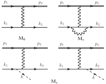
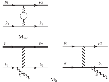
Figure 1: Feynman’s diagrams corresponding to the Born approximation and first order virtual radiative corrections (top), and to initial and final real photon emission, $M_{s}$ (soft) and $M_{h}$ (hard), from the lepton vertex (bottom).

II Formalism

Let us consider the reaction

$$p(p_{1})+e(k_{1})\to p(p_{2})+e(k_{2}),$$ (1)

where the particle momenta are indicated in parenthesis, and $q=k_{1}-k_{2}=p_{2}-p_{1}$ is the four momentum of the virtual photon.

II.1 Inverse kinematics

A general characteristic of all reactions of elastic and inelastic hadron scattering by atomic electrons (which can be considered at rest) is the small value of the momentum transfer squared, even for relatively large energies of the colliding particles. Let us give details of the order of magnitude and the dependence of the kinematic variables, as they are very specific for these reactions. In particular, the electron mass can not be neglected in the kinematics and dynamics of the reaction, even when the beam energy is of the order of GeV.

One can show that, for a given energy of the proton beam, the maximum value of the four momentum transfer squared, in the scattering on electrons at rest, is

$$(Q^{2})_{max}=\frac{4m^{2}\vec{p}^{2}}{M^{2}+2mE+m^{2}},$$ (2)

where m(M) is the electron (proton) mass, $E(\vec{p})$ is the energy (momentum) of the proton beam. Being proportional to the electron mass squared, the four momentum transfer squared is restricted to very small values, where the proton can be considered structureless.

The four momentum transfer squared is expressed as a function of the energy of the scattered electron, $\epsilon_{2}$, as: $q^{2}=(k_{1}-k_{2})^{2}=2m(m-\epsilon_{2})$, where

$$\epsilon_{2}=m\frac{(E+m)^{2}+\vec{p}^{2}\cos^{2}\theta_{e}}{(E+m)^{2}-\vec{p}^{2}\cos^{2}\theta_{e}},$$ (3)

where $\theta_{e}$ is the angle between the proton beam and the scattered electron momenta.

From energy and momentum conservation, one finds the following relation between the angle and the energy of the scattered electron:

$$\cos\theta_{e}=\displaystyle\frac{(E+m)(\epsilon_{2}-m)}{|\vec{p}|\sqrt{\epsilon_{2}^{2}-m^{2}}},$$ (4)

which shows that $\cos\theta_{e}\geq 0$ (the electron can never be scattered backward). One can see from Eq. (3) that, in inverse kinematics, the available kinematical region is reduced to small values of $\epsilon_{2}$:

$$\epsilon_{2,max}=m\frac{2E(E+m)+m^{2}-M^{2}}{M^{2}+2mE+m^{2}},$$ (5)

which is proportional to the electron mass. From the momentum conservation, on can find the following relation between the energy and the angle of the scattered proton $E_{2}$ and $\theta_{p}$:

$$E_{2}^{\pm}=\frac{(E+m)(M^{2}+mE)\pm M\vec{p}^{2}\cos\theta_{p}\sqrt{\frac{m^{2}}{M^{2}}-\sin^{2}\theta_{p}}}{(E+m)^{2}-\vec{p}^{2}\cos^{2}\theta_{p}},$$ (6)

showing that, for one proton angle, there may be two values of the proton energies, (and two corresponding values for the recoil-electron energy and angle as well as for the transferred momentum $q^{2}$). This is a typical situation when the center-of-mass velocity is larger than the velocity of the projectile in the center of mass, where all the angles are allowed for the recoil electron. The two solutions coincide when the angle between the initial and final hadron takes its maximum value, which is determined by the ratio of the electron and scattered hadron masses $M_{h}$, $\sin\theta_{h,max}=m/M_{h}$. One concludes that hadrons are scattered on atomic electrons at very small angles, and that the larger is the hadron mass, the smaller is the available angular range for the scattered hadron.

II.2 Differential cross section

In the one-photon exchange (Born) approximation, the matrix element ${\cal M}^{(B)}$ of the reaction (1) can be written as:

$${\cal M}^{(B)}=\frac{e^{2}}{q^{2}}j_{\mu}J_{\mu},$$ (7)

where $j_{\mu}(J_{\mu})$ is the leptonic (hadronic) electromagnetic current:

$$j_{\mu} = \bar{u}(k_{2})\gamma_{\mu}u(k_{1}),$$ (8)

$$J_{\mu} = \bar{u}(p_{2})\left[F_{1}(q^{2})\gamma_{\mu}-\frac{1}{2M}F_{2}(q^{2})\sigma_{\mu\nu}q_{\nu}\right]u(p_{1})=$$

$$= \bar{u}(p_{2})\left[G_{M}(q^{2})\gamma_{\mu}-F_{2}(q^{2})P_{\mu}\right]u(p_{1}),$$

where $P_{\mu}=(p_{1}+p_{2})_{\mu}/(2M)$. $F_{1}(q^{2})$ and $F_{2}(q^{2})$ are the Dirac and Pauli proton electromagnetic form factors, $G_{M}(q^{2})=F_{1}(q^{2})+F_{2}(q^{2})$ is the Sachs proton magnetic form factor. The matrix element squared is written as:

$$|{\cal M}^{(B)}|^{2}=16\pi^{2}\frac{\alpha^{2}}{q^{4}}L_{\mu\nu}W_{\mu\nu},\mbox{~{}with~{}}L_{\mu\nu}=j_{\mu}j_{\nu}^{*},~{}W_{\mu\nu}=J_{\mu}J_{\nu}^{*},$$ (9)

where $\alpha=e^{2}/(4\pi)=1/137$ is the electromagnetic fine structure constant. The leptonic tensor, $L_{\mu\nu}$, for unpolarized initial and final electrons (averaging over the initial electron spin) has the form:

$$L_{\mu\nu}=q^{2}g_{\mu\nu}+2(k_{1\mu}k_{2\nu}+k_{1\nu}k_{2\mu}).$$ (10)

The hadronic tensor $W_{\mu\nu}$, for unpolarized initial and final protons can be written in the standard form, through two unpolarized structure functions:

$$W_{\mu\nu}=\left(-g_{\mu\nu}+\frac{q_{\mu}q_{\nu}}{q^{2}}\right)W_{1}(q^{2})+P_{\mu}P_{\nu}W_{2}(q^{2}).$$ (11)

Averaging over the initial proton spin, the structure functions $W_{i}$, $i=1,2$, are expressed in terms of the nucleon electromagnetic form factors:

$$W_{1}(q^{2})=-q^{2}G_{M}^{2}(q^{2}),\ \ W_{2}(q^{2})=4M^{2}\frac{G_{E}^{2}(q^{2})+\tau G_{M}^{2}(q^{2})}{1+\tau},$$ (12)

where $G_{E}(q^{2})=F_{1}(q^{2})-\tau F_{2}(q^{2})$ is the proton electric form factor and $\tau=-q^{2}/4M^{2}$.

The expression of the differential cross section, as a function of the recoil-electron energy $\epsilon_{2}$, for unpolarized proton-electron scattering can be written as:

$$\frac{d\sigma^{(B)}}{d\epsilon_{2}}=\frac{\pi\alpha^{2}}{m\vec{p}^{2}}\frac{\cal D}{q^{4}},$$ (13)

with

$${\cal D}=q^{2}(q^{2}+2m^{2})G_{M}^{2}(q^{2})+2\left[q^{2}M^{2}+\frac{1}{1+\tau}\left(2mE+\frac{q^{2}}{2}\right)^{2}\right]\left[G_{E}^{2}(q^{2})+\tau G_{M}^{2}(q^{2})\right].$$ (14)

This expression is valid in the one-photon exchange (Born) approximation in the reference system where the target electron is at rest.

The expression of the differential cross section, as a function of the four-momentum transfer squared, is

$$\frac{d\sigma^{(B)}}{dq^{2}}=\frac{\pi\alpha^{2}}{2m^{2}\vec{p}^{2}}\frac{\cal D}{q^{4}}.$$ (15)

And at last, the differential cross section over the scattered-electron solid angle has the following expression

$$\frac{d\sigma^{(B)}}{d\Omega_{e}}=\frac{\alpha^{2}}{8m^{4}|\vec{p}|}\left(1-\frac{4m^{2}}{q^{2}}\right)^{3/2}\frac{\cal D}{E+m}.$$ (16)

III Radiative corrections

Let us consider the model-independent QED radiative corrections which are due to the vacuum polarization and emission of the virtual and real (soft and hard) photons in the electron vertex. The corresponding diagrams are shown in Fig.1.

III.1 Soft photon emission

In this section we calculate the contribution to the radiative corrections of the soft photon emission when the photons are emitted by the initial and final electrons

$$p(p_{1})+e(k_{1})\to p(p_{2})+e(k_{2})+\gamma(k).$$ (17)

The matrix element in this case (the photon emitted from the electron vertex) is given by

$${\cal M}^{(\gamma)}=\frac{1}{q^{2}}(4\pi\alpha)^{3/2}j_{\mu}^{(\gamma)}J_{\mu},$$ (18)

where the electron current corresponding to the photon emission is

$$j_{\mu}^{(\gamma)}=\bar{u}(k_{2})\left[\frac{1}{d_{1}}\gamma_{\mu}(\hat{k}_{1}-\hat{k}+m)\gamma_{\rho}+\frac{1}{d_{2}}\gamma_{\rho}(\hat{k}_{2}+\hat{k}+m)\gamma_{\mu}\right]u(k_{1})A^{*}_{\rho},$$ (19)

where $A_{\rho}$ is the polarization vector of the emitted photon and $d_{1}=-2k\cdot k_{1},d_{2}=2k\cdot k_{2}$.

The differential cross section of reaction (17) can be written as

$$d\sigma^{(\gamma)}=\frac{(2\pi)^{-5}}{32m|\vec{p}|}|{\cal M}^{(\gamma)}|^{2}\frac{d^{3}\vec{k}_{2}}{\epsilon_{2}}\frac{d^{3}\vec{p}_{2}}{E_{2}}\frac{d^{3}\vec{k}}{\omega}\delta^{4}(k_{1}+p_{1}-k_{2}-p_{2}-k).$$ (20)

It is necessary to integrate over the photon phase space. Since the photons are assumed to be soft, then the integration over the photon energy is restricted to $\omega\leq\bar{\omega}$. The quantity $\bar{\omega}$ is determined by particular experimental conditions and it is assumed that $\bar{\omega}$ is sufficiently small to neglect the momentum $k$ in the $\delta$ function and in the numerators of the matrix element ${\cal M}^{(\gamma)}$. In order to avoid the infrared divergence, which occurs in the soft photon cross section, a small fictitious photon mass $\lambda$ is introduced.

In the soft photon approximation, the matrix element (18) is

$${\cal M}^{(\rm soft)}=\sqrt{4\pi\alpha}\left(\frac{k_{2}\cdot A^{*}}{k\cdot k_{2}}-\frac{k_{1}\cdot A^{*}}{k\cdot k_{1}}\right){\cal M}^{(B)}.$$ (21)

The differential cross section (20), integrated over the soft photon phase space, can be written as

$$d\sigma^{(\rm soft)}=\delta^{(s)}d\sigma^{(B)},$$ (22)

where the radiative correction due to the soft photon emission is

$$\delta^{(s)}=-\frac{\alpha}{4\pi^{2}}\int_{\lambda}^{\bar{\omega}}\sqrt{\omega^{2}-\lambda^{2}}d\omega\int d\Omega_{k}\Bigl{[}\frac{m^{2}}{(k\cdot k_{1})^{2}}+\frac{m^{2}}{(k\cdot k_{2})^{2}}-2\frac{k_{1}\cdot k_{2}}{k\cdot k_{1}k\cdot k_{1}}\Bigr{]}.$$ (23)

Assuming $\bar{\omega}\ll m$ and using the results of the paper ’t Hooft and Veltman (1979), we can do the integration and the expression for $\delta^{(s)}$ has the form

$$\delta^{(s)} = \frac{\alpha}{\pi}\left\{1-2\ln{\frac{2\bar{\omega}}{\lambda}}+\frac{\epsilon_{2}}{k_{2}}\left[\ln{\frac{\epsilon_{2}+k_{2}}{m}}\left(1+2\ln{\frac{2\bar{\omega}}{\lambda}}+\ln{\frac{\epsilon_{2}+k_{2}}{m}}+2\ln{\frac{m}{2k_{2}}}\right)-\right.\right.$$ (24)

$$\left.\left.-\frac{\pi^{2}}{6}+Li_{2}\left(\frac{\epsilon_{2}-k_{2}}{\epsilon_{2}+k_{2}}\right)\right]\right\},$$

where $k_{2}\equiv|\vec{k}_{2}|$ ($\vec{k}_{2}$ is the momentum of the recoil electron) and $Li_{2}(x)$ is the Spence (dilogarithm) function defined as

$$Li_{2}(x)=-\int_{0}^{x}\frac{\ln{(1-t)}}{t}dt.$$

III.2 Virtual photon emission

In this section, we calculate the contribution to the radiative corrections of the virtual photon emission in the electron vertex (the electron vertex correction) and the vacuum polarization term.

The matrix element corresponding to this process can be written as

$${\cal M}^{(\rm virt)}=\frac{1}{q^{2}}4\pi\alpha J_{\mu}\bar{u}(k_{2})\Lambda_{\mu}(k_{1},k_{2})u(k_{1}),$$ (25)

where we introduce

$$\Lambda_{\mu}(k_{1},k_{2})=\frac{2i\alpha}{(2\pi)^{3}}\int\frac{d^{4}k}{k^{2}-\lambda^{2}}\frac{\hat{O}_{\mu}}{(k^{2}-2k\cdot k_{1})(k^{2}-2k\cdot k_{2})}$$ (26)

and the matrix $\hat{O}_{\mu}$ is

$$\hat{O}_{\mu}=4k_{1}\cdot k_{2}\gamma_{\mu}-2(\hat{k}_{1}\hat{k}\gamma_{\mu}+\gamma_{\mu}\hat{k}\hat{k}_{2})-2\hat{k}\gamma_{\mu}\hat{k}.$$ (27)

The integration over the virtual-photon four-momentum $k$ leads to the following expression for the function $\Lambda_{\mu}(k_{1},k_{2})$

$$\Lambda_{\mu}(k_{1},k_{2}) = \frac{\alpha}{4\pi}\left\{\left[\ln\frac{\Lambda^{2}}{m^{2}}+\frac{1}{2}+\int_{0}^{1}\frac{dx}{P^{2}_{x}}\left(4m^{2}-\frac{3}{2}q^{2}+(q^{2}-2m^{2})\left(\ln\frac{P^{2}_{x}}{m^{2}}+\ln\frac{m^{2}}{\lambda^{2}}\right)\right)\right]\right.\gamma_{\mu}$$ (28)

$$\left.+m\int_{0}^{1}\frac{dx}{P^{2}_{x}}\sigma_{\mu\nu}q_{\nu}\right\},$$

where $P^{2}_{x}=m^{2}-x(1-x)q^{2}$ and $\Lambda$ is the cut parameter which define the region of infinite momenta of the virtual photon. Thus we avoid the ultraviolet divergence. The regularized vertex function can be obtained by the subtraction of the contribution

$$\Lambda_{\mu}(k_{1},k_{1})=\frac{\alpha}{4\pi}\gamma_{\mu}\left[\ln\frac{\Lambda^{2}}{m^{2}}+\frac{9}{2}-2\ln\frac{m^{2}}{\lambda^{2}}\right]$$

from the expression (28). As a result, we have

$$\Lambda^{R}_{\mu}(k_{1},k_{2})=\Lambda_{\mu}(k_{1},k_{2})-\Lambda_{\mu}(k_{1},k_{1})=\frac{\alpha}{4\pi}(A\gamma_{\mu}+B\sigma_{\mu\nu}q_{\nu}),$$ (29)

where

$$A=-4+2\ln\frac{m^{2}}{\lambda^{2}}+\int_{0}^{1}\frac{dx}{P^{2}_{x}}\left\{4m^{2}-\frac{3}{2}q^{2}+(q^{2}-2m^{2})\left[\ln\frac{P^{2}_{x}}{m^{2}}+\ln\frac{m^{2}}{\lambda^{2}}\right]\right\},\ \ B=m\int_{0}^{1}\frac{dx}{P^{2}_{x}}.$$ (30)

As we limit ourselves to the calculation of the radiative corrections at the order of $\alpha$ in comparison with the Born term, it is sufficient to calculate the interference of the Born matrix element with ${\cal M}^{(virt)}$

$$|{\cal M}|^{2}=|{\cal M}^{(B)}|^{2}+2Re[{\cal M}^{(\rm virt)}{\cal M}^{(B)*}]=(1+\delta_{1}+\delta_{2})|{\cal M}^{(B)}|^{2},$$ (31)

where the term $\delta_{1}$ is due to the modification of the $\gamma_{\mu}$ term in the electron vertex, and the term $\delta_{2}$ is due to the presence of the $\sigma_{\mu\nu}q_{\nu}$ structure in the electron vertex.

The integration over the $x$ variable in the expression (30) gives the following results for the radiative corrections due to the emission of the virtual photon in the electron vertex

$$\delta_{1} = \frac{\alpha}{\pi}\left\{-2+2\ln\frac{m}{\lambda}\left[1-\frac{\epsilon_{2}}{k_{2}}\ln\left(\frac{\epsilon_{2}+k_{2}}{m}\right)\right]+\frac{m+3\epsilon_{2}}{2k_{2}}\ln\left(\frac{\epsilon_{2}+k_{2}}{m}\right)-\frac{1}{2}\frac{\epsilon_{2}}{k_{2}}\ln\left(\frac{Q^{2}}{m^{2}}\right)\ln\left(\frac{\epsilon_{2}+k_{2}}{m}\right)+\right.$$

$$\left.+\frac{\epsilon_{2}}{k_{2}}\left[-\ln\left(\frac{m+\epsilon_{2}}{k_{2}}\right)\ln\left(\frac{\epsilon_{2}+k_{2}}{m}\right)+Li_{2}\left(\frac{\epsilon_{2}+k_{2}+m}{2\left(m+\epsilon_{2}\right)}\right)-Li_{2}\left(\frac{\epsilon_{2}-k_{2}+m}{2\left(m+\epsilon_{2}\right)}\right)\right]\right\},$$

$$\delta_{2} = 4\frac{\alpha}{\pi}\frac{mM^{2}q^{2}}{k_{2}{\cal D}}\ln\left(\frac{\epsilon_{2}+k_{2}}{m}\right)(G_{E}^{2}-2\tau G_{M}^{2}).$$ (32)

The radiative correction due to the vacuum polarization is (the electron loop has been taken into account):

$$\delta^{(\rm vac)}=\frac{2\alpha}{3\pi}\left\{-\frac{5}{3}+4\frac{m^{2}}{Q^{2}}+(1-2\frac{m^{2}}{Q^{2}})\sqrt{1+4\frac{m^{2}}{Q^{2}}}\ln\frac{\sqrt{1+4\frac{m^{2}}{Q^{2}}}+1}{\sqrt{1+4\frac{m^{2}}{Q^{2}}}-1}\right\}.$$ (33)

For small and large values of the $Q^{2}$ variable we have

$$\mbox{If \ \ }Q^{2}\ll m^{2},\ \ \ \delta^{(\rm vac)}=\frac{2\alpha}{15\pi}\frac{Q^{2}}{m^{2}},$$

$$\mbox{If \ \ }\ \ Q^{2}\gg m^{2},\ \ \ \delta^{(\rm vac)}=\frac{2\alpha}{3\pi}\left[-\frac{5}{3}+\ln\frac{Q^{2}}{m^{2}}\right].$$

Taking into account the radiative corrections given by Eqs. (24, 32, 33), we obtain the following expression for the differential cross section:

$$d\sigma^{(RC)}=(1+\delta_{1}+\delta_{2}+\delta^{(s)}+\delta^{(\rm vac)})d\sigma^{(B)}=(1+\delta_{0}+\bar{\delta}+\delta^{(\rm vac)})d\sigma^{(B)},$$ (34)

where the radiative corrections $\delta_{0}$ and $\bar{\delta}$ are given by

$$\delta_{0} = \frac{2\alpha}{\pi}\ln\frac{\bar{\omega}}{m}\left[\frac{\epsilon_{2}}{k_{2}}\ln\left(\frac{\epsilon_{2}+k_{2}}{m}\right)-1\right],$$

$$\bar{\delta} = \frac{\alpha}{\pi}\left\{-1-2\ln 2+\frac{\epsilon_{2}}{k_{2}}\left[\ln\left(\frac{\epsilon_{2}+k_{2}}{m}\right)\left(1+\ln\left(\frac{\epsilon_{2}+k_{2}}{m}\right)+2\ln\left(\frac{m}{k_{2}}\right)+\frac{m+3\epsilon_{2}}{2\epsilon_{2}}-\right.\right.\right.$$ (35)

$$\left.-\ln\left(\frac{\epsilon_{2}+m}{k_{2}}\right)-\frac{1}{2}\ln\left(\frac{Q^{2}}{m^{2}}\right)\right)+4m\frac{M^{2}q^{2}}{\epsilon_{2}{\cal D}}\ln\left(\frac{\epsilon_{2}+k_{2}}{m}\right)(G_{E}^{2}-2\tau G_{M}^{2})-$$

$$\left.\left.-\frac{\pi^{2}}{6}+Li_{2}\left(\frac{\epsilon_{2}-k_{2}}{\epsilon_{2}+k_{2}}\right)+Li_{2}\left(\frac{\epsilon_{2}+k_{2}+m}{2(\epsilon_{2}+m)}\right)-Li_{2}\left(\frac{\epsilon_{2}-k_{2}+m}{2(\epsilon_{2}+m)}\right)\right]\right\}.$$

We separate the contribution $\delta_{0}$ since it can be summed up in all orders of the perturbation theory using the exponential form of the electron structure functions Kuraev and Fadin (1985). To do this it is sufficient to keep only the exponential contributions in the electron structure functions. The final result can be obtained by the substitution of the term $(1+\delta_{0})$ by the following term

$$\left(\displaystyle\frac{\bar{\omega}}{m}\right)^{\beta}\displaystyle\frac{\beta}{2}\int_{0}^{1}x^{\frac{\beta}{2}-1}(1-x)^{\frac{\beta}{2}}dx,$$ (36)

where

$$\beta=\displaystyle\frac{2\alpha}{\pi}\left[\frac{\epsilon_{2}}{k_{2}}\ln\left(\displaystyle\frac{\epsilon_{2}+k_{2}}{m}\right)-1\right].$$

III.3 Hard photon emission

In this section we calculate the radiative correction due to the hard photon emission by the initial and recoil electrons only (the model-independent part). The contribution due to radiation from the initial and scattered protons (the model-dependent part) requires a special consideration and we leave it for other investigations. We consider the experimental setup when only the energies of the scattered proton and final electron are measured.

The differential cross section of the reaction (17), averaged over the initial particle spins, can be written as

$$d\,\sigma^{(h)}=\frac{\alpha^{3}}{32\,\pi^{2}}\,\frac{1}{m\,p}\,\frac{L_{\mu\nu}^{(\gamma)}\,W_{\mu\nu}}{q_{1}^{4}}\frac{d^{3}k_{2}}{\epsilon_{2}}\frac{d^{3}p_{2}}{E_{2}}\frac{d^{3}k}{\omega}\delta(p_{1}+k_{1}-p_{2}-k_{2}-k),$$ (37)

where $q_{1}=k_{1}-k_{2}-k$ and the leptonic tensor has the following form

$$L_{\mu\nu}^{(\gamma)} = A_{0}\tilde{g}_{\mu\nu}+A_{1}\tilde{k}_{1\mu}\tilde{k}_{1\nu}+A_{2}\tilde{k}_{2\mu}\tilde{k}_{2\nu}+A_{12}(\tilde{k}_{1\mu}\tilde{k}_{2\nu}+\tilde{k}_{1\nu}\tilde{k}_{2\mu})\,,$$ (38)

$$A_{0} = 4\left[\frac{d_{1}}{d_{2}}+\frac{d_{2}}{d_{1}}-2q_{1}^{2}\left(\frac{m^{2}}{d_{1}^{2}}+\frac{m^{2}}{d_{2}^{2}}+2\frac{k_{1}\cdot k_{2}}{d_{1}d_{2}}\right)\right],\ A_{1}=16\frac{q_{1}^{2}}{d_{1}d_{2}}-32\frac{m^{2}}{d_{2}^{2}},$$

$$A_{2} = 16\frac{q_{1}^{2}}{d_{1}d_{2}}-32\frac{m^{2}}{d_{1}^{2}},\ A_{12}=-32\frac{m^{2}}{d_{1}d_{2}}\,.$$

The hadronic tensor is defined by Eqs.(11 ,12) with the substitution $q\to q_{1}.$

The contraction of leptonic and hadronic tensors reads

$$L_{\mu\nu}^{(\gamma)}W_{\mu\nu}=-W_{1}(q_{1}^{2})\,S_{1}+\frac{W_{2}(q_{1}^{2})}{M^{2}}\,S_{2}\,,$$ (39)

where the functions $S_{1,2}$ have the following expressions

$$S_{1} = 8\left(\frac{d_{1}}{d_{2}}+\frac{d_{2}}{d_{1}}\right)-\frac{16}{d_{1}d_{2}}(2m^{2}+q_{1}^{2})\left[2k_{1}\cdot k_{2}+m^{2}\left(\frac{d_{1}}{d_{2}}+\frac{d_{2}}{d_{1}}\right)\right]\,,$$ (40)

$$S_{2} = 4M^{2}\left[\frac{d_{1}}{d_{2}}+\frac{d_{2}}{d_{1}}-2q_{1}^{2}\left(\frac{m^{2}}{d_{1}^{2}}+\frac{m^{2}}{d_{2}^{2}}+2\frac{k_{1}\cdot k_{2}}{d_{1}d_{2}}\right)\right]+32\frac{m^{2}}{d_{1}d_{2}}(k\cdot p_{1})^{2}+16\frac{(k_{1}\cdot p_{1})^{2}}{d_{1}}+$$ (41)

$$+16\frac{(k_{2}\cdot p_{1})^{2}}{d_{2}}+16k_{1}\cdot p_{1}k_{2}\cdot p_{1}\left[\frac{1}{d_{1}}+\frac{1}{d_{2}}-2\left(\frac{m^{2}}{d_{1}^{2}}+\frac{m^{2}}{d_{2}^{2}}+2\frac{k_{1}\cdot k_{2}}{d_{1}d_{2}}\right)\right]+$$

$$+16k\cdot p_{1}\left[\frac{k_{1}\cdot p_{1}}{d_{2}^{2}}(d_{2}-2m^{2})-\frac{k_{2}\cdot p_{1}}{d_{1}^{2}}(d_{1}-2m^{2})+2\frac{k_{1}\cdot k_{2}}{d_{1}d_{2}}(k_{2}\cdot p_{1}-k_{1}\cdot p_{1})\right].$$

Integrating over the scattered proton variables we obtain the following expression for the differential cross section

$$d\sigma^{(h)}=\frac{\alpha^{3}}{32\pi^{2}}\frac{1}{m\,p}\int\frac{d^{3}{k}}{\omega}\int\frac{d^{3}{k}_{2}}{\epsilon_{2}\,E_{2}}\frac{1}{q_{1}^{4}}L_{\mu\nu}^{(\gamma)}W_{\mu\nu}\,\delta(m+E-\epsilon_{2}-E_{2}-\omega)\,.$$ (42)

To integrate further we have to define the coordinate system. Following Ref. Kahane (1964), where the $\pi-e^{-}$ scattering has been analyzed, let us take the $z$-axis along the vector $\vec{p}-\vec{k}$ and the momenta of the initial proton and emitted photon lie in the $xz$ plane. The momentum of the scattered electron is defined by the polar $\theta$ and azimuthal $\varphi$ angles as it is shown in Fig.2. The angle $\eta(\phi)$ is the angle between the beam direction and $z$ axis (emitted photon momentum).

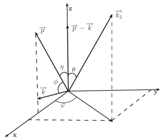
Figure 2: Coordinate system and definition of the angles used for the integration over the variables of the final state.

Integrating over the polar angle of the scattered electron we obtain:

$$\frac{d\sigma^{(h)}}{d\epsilon_{2}}=\frac{\alpha^{3}}{32\pi^{2}}\frac{1}{m\,p}\int\frac{d^{3}\,k}{\omega}\int\frac{d\varphi}{|\vec{p}-\vec{k}|}\,\frac{1}{q_{1}^{4}}L_{\mu\nu}^{(\gamma)}\,W_{\mu\nu}.$$ (43)

The region of allowed photon momenta should be determined. The experiment counts those events which, within the accuracy of the detectors, are considered ”elastic”. We refer to the experimental situation where the energies of the scatted proton and recoil electron are measured. Because of the uncertainties in determination of the recoil electron ($\Delta\epsilon_{2}$) and scattered proton ($\Delta E_{2}$) energies, which usually are proportional to $\epsilon_{2}$ and $E_{2},$ respectively, the elastic proton-electron scattering always accompanied by the hard photon emission with the energies up to $\Delta\epsilon_{2}+\Delta E_{2}$. At the proton beam energies of the order of 100 GeV this value can reach a few GeV. The events for which the scattered proton energy is $E_{2}\pm\Delta E_{2}$ and the recoil electron energy is $\epsilon_{2}\pm\Delta\epsilon_{2}$ (they satisfy the condition $E+m=E_{2}+\epsilon_{2}$) are considered as true elastic events. Here, $\Delta E_{2}$ and $\Delta\epsilon_{2}$ are the errors in the measurement of the final proton and recoil electron energies. The plot of the variable $E_{2}$ versus the variable $\epsilon_{2}$ is shown in Fig.3. The shaded area in this figure represents those events allowed by the experimental limitations. The relation between the energies $E_{2}$ and $\epsilon_{2}$, as it is shown in Fig.3, has to be transformed into a limit on the possible photon momentum $\vec{k}$. We consider the experimental setup where no angles are measured and, therefore, the orientation of the photon momentum $\vec{k}$ is not limited. In our calculation we restrict ourselves with the region $\epsilon_{2}<\epsilon_{2max}-\Delta E,$ where $\Delta E=\Delta E_{2}+\Delta\epsilon_{2}$ and $\epsilon_{2max}$ is defined by Eq. (5). In this case we get for the experimental restriction the isotropic condition

$$\omega\leq\Delta E.$$

In other case $\epsilon_{2}>\epsilon_{2max}-\Delta E$, the restriction for the photon energy is

$$\omega\leq\epsilon_{2max}-\epsilon_{2}.$$

Figure 3: Plane of the $E_{2}$ and $\epsilon_{2}$ variables where the shaded area represents the kinematically allowed region within the experimental set-up.

In the chosen coordinate system the element of solid angle becomes: $d^{3}k\to 2\pi\,\omega^{2}\,d\omega\,d\cos{\phi}.$ Now we introduce a new variable $y=E-p\cos{\phi}>0$ and rewrite Eq. (43) as

$$\frac{d\sigma^{(h)}}{d\epsilon_{2}}=\frac{\alpha^{3}}{16\,\pi}\frac{1}{m\,p^{2}}\int\omega\,d\omega\int d\,y\int\limits_{0}^{2\pi}\frac{1}{q_{1}^{4}\,|\vec{p}-\vec{k}|}\Big{(}-W_{1}(q_{1}^{2})\,S_{1}+\frac{W_{2}(q_{1}^{2})}{M^{2}}\,S_{2}\Big{)}d\,\varphi\,,$$ (44)

where the integration region over the variables $\omega$ and $y$ is shown in Fig.4, and

$$\omega_{s}=(|\vec{k}_{2}|-|\vec{p}|+x)\frac{M^{2}|\vec{k}_{2}|(|\vec{k}_{2}|+|\vec{p}|)+(m-\epsilon_{2})[M^{2}(x-m)+2m(2Ex+m^{2}-m\epsilon_{2})]}{4(m-\epsilon_{2})[x(M^{2}+m^{2}+2mE)-m(M^{2}+mE)]+M^{4}},$$ (45)

where $x=E+m-\epsilon_{2}.$

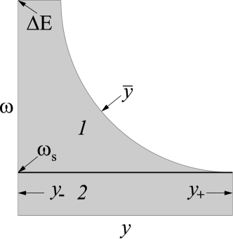
Figure 4: Integration region over the variables $\omega$ and $y$. Here $y_{\pm}=E\pm p,~{}\bar{y}=[(m-\epsilon_{2})(E-\epsilon_{2}-\omega)+\sqrt{\epsilon_{2}^{2}-m^{2}}\sqrt{(E+m-\epsilon_{2}-\omega)^{2}-M^{2}}]/\omega.$ The quantity $\omega_{s}$ is defined by positive solution of the equation $\bar{y}=y_{+}$ and given by Eq. (45).

The quantity $\omega_{s}$ represents the maximal energy, when the photon can be emitted in the whole angular phase space. The dependence of this quantity on the recoil electron energy, at different values of the proton beam energy, is shown in Fig.5. We see that it is of the order of the electron mass $m$ in a wide range of the energies $\epsilon_{2}$ and $E$. Because our analytical calculations for the soft photon correction were performed under the condition $\bar{\omega}\ll m,$ where $\bar{\omega}$ is the maximal energy of the soft photon, we can not identify $\omega_{s}$ with $\bar{\omega}\ll m,$ as it has been done in the paper Kahane (1964).

Figure 5: Maximum energy of the photon, when emitted in the whole angular phase space.

Following the Ref. Kahane (1964), we include in the integral (44) the weight function $g(\omega)$ given by

$$g(\omega)=1\ \ \mbox{for}\ \ \bar{\omega}<\omega<\Delta E_{2}-\Delta\epsilon_{2},$$

$$g(\omega)=\frac{\Delta E_{2}+\Delta\epsilon_{2}-\omega}{2\Delta\epsilon_{2}}\ \ \mbox{for}\ \ \Delta E_{2}-\Delta\epsilon_{2}<\omega<\Delta E_{2}+\Delta\epsilon_{2}\,.$$

In fact, the function $g(\omega)$ is the ratio of the straight line segments cut by the lines $E_{2}+\epsilon_{2}+\omega=E+m$ and $E_{2}+\epsilon_{2}=E+m$ in the shaded region in Fig.3.

So, the expression for the cross section given by Eq. (44) can be written as a sum of two terms

$$\frac{d\sigma^{(h)}}{d\epsilon_{2}}=\frac{\alpha^{3}}{16\,\pi}\frac{1}{m\,p^{2}}\bigg{[}\int\limits_{\omega_{s}}^{\Delta E}g(\omega)\,C_{1}(\omega)\,d\omega+\int\limits_{\bar{\omega}}^{\omega_{s}}C_{2}(\omega)\,d\omega\bigg{]}\,,$$ (46)

where

$$C_{1}(\omega) = \int\limits_{y_{-}}^{\bar{y}}\int\limits_{0}^{2\pi}\left[\frac{\omega}{q_{1}^{4}\,|\vec{p}-\vec{k}|}\left(-W_{1}(q_{1}^{2})\,S_{1}+\frac{W_{2}(q_{1}^{2})}{M^{2}}\,S_{2}\right)\right]d\varphi dy,$$

$$C_{2}(\omega) = \int\limits_{y_{-}}^{y_{+}}\int\limits_{0}^{2\pi}\left(\frac{\omega}{q_{1}^{4}\,|\vec{p}-\vec{k}|}\left(-W_{1}(q_{1}^{2})\,S_{1}+\frac{W_{2}(q_{1}^{2})}{M^{2}}\,S_{2}\right)\right]d\varphi dy.$$ (47)

The scalar products of various 4-momenta, which enter in the expressions for $S_{1},S_{2}$ and $q_{1}^{2}$, are expressed, in terms of the angles, as illustrated in Fig.2, and the photon energy, as follows:

$$d_{1} = -2m\,\omega\,,\ \ k_{1}\cdot k_{2}=m\,\epsilon_{2}\,,\ k_{1}\cdot p_{1}=m\,E\,,\ \ k\cdot p_{1}=\omega(E-p\cos{\phi})\,,$$

$$d_{2} = 2\,\omega[\epsilon_{2}-|\vec{k}_{2}|(\cos{\theta}\,\cos{(\eta+\phi)}+\cos{\varphi}\sin{\theta}\,\sin{(\eta+\phi)})]\,,$$ (48)

$$k_{2}\cdot p_{1} = \epsilon_{2}\,E-p|\vec{k}_{2}|(\cos{\eta}\cos{\theta}+\cos{\varphi}\sin{\eta}\sin{\theta})\,.$$

In turn, the respective trigonometric functions of angles are expressed through the photon energy and the variable $y,$ as:

$$\cos{\eta} = \frac{p^{2}-\omega(E-y)}{p|\vec{p}-\vec{k}|}\,,\ \ \cos{(\eta+\phi)}=\frac{E-\omega-y}{|\vec{p}-\vec{k}|}\,,$$

$$\cos{\theta} = \frac{(\epsilon_{2}-m)(E+m)+\omega(y+m-\epsilon_{2})}{|\vec{p}-\vec{k}|}\,,\ \ \sin{\theta}\,,\ \sin{\eta}\,,\ \sin{(\eta+\phi)}\geq 0\,,$$ (49)

$$|\vec{p}-\vec{k}| = \sqrt{p^{2}+\omega(2y-2E+\omega)}\,.$$

The functions $W_{1}$ and $W_{2}$ depend on the azimuthal angle $\varphi$, and, in order to perform the integration over this variable in the r.h.s. of Eq.(46), one needs to use a specific expressions for the form factors entering these functions. Further we concentrate on small values of the squared momentum transfer as compared with the proton mass, where the form factors can be expanded in a series in term of powers of $q_{1}^{2}.$ In the calculations we keep the terms of the order of $1\,,$ $q_{1}^{2}$, and $q_{1}^{4}$ in the quantity

$$-W_{1}(q_{1}^{2})\,S_{1}+\frac{W_{2}(q_{1}^{2})}{M^{2}}\,S_{2}$$

which enters the differential cross section.

The integration in the r.h.s. of Eq. (46) over the $\varphi$ and $y$ variables is performed analytically. The result for both $C_{1}(\omega)$ and $C_{2}(\omega)$ is very cumbersome, and it was published in the Appendix of our preprint Gakh et al. (2016). In the limit $\omega\to 0$ the function $C_{1}(\omega)$ is regular, and the function $C_{2}(\omega)$ has an infrared behaviour. We extract the regular part $C_{2R}(\omega)$ and the infrared contribution $C_{2I}(\omega)$ by a simple subtraction procedure, by writing

$$C_{2}(\omega)=\big{[}C_{2}(\omega)-C_{2}(\omega\to 0)\big{]}+C_{2}(\omega\to 0)=C_{2R}(\omega)+C_{2I}(\omega)\,,\ \ C_{2I}(\omega)\sim\frac{1}{\omega}\left[\frac{\epsilon_{2}}{k_{2}}\ln\frac{\epsilon_{2}+k_{2}}{m}-1\right]\,.$$ (50)

The infrared contribution is combined with the correction due to soft and virtual photon emission and this results in change $\bar{\omega}\to\omega_{s}$ in the expression for $\delta_{0}$ (see Eq. (35)). The integration of the regular part $C_{2R}(\omega)$ over $\omega$ (as the lower limit we can chose an arbitrary small value) as well the whole contribution of the region 1, $C_{1}(\omega),$ is performed numerically.

IV Numerical estimations and discussion

In the following section the conditions for the experimental uncertainties are set to: $\Delta E_{2}=0.02E$ and $\Delta\epsilon_{2}=0.03\epsilon_{2}$ if other choice is not specified.

Since the four-momentum transfer squared is very small in this reaction, the proton charge and magnetic form factors are approximated by Taylor series expansions. We use the expansion over the variable $q^{2}$ of three form factor parameterizations.

By means of the radii (labeled as (r)). In this approach we use the expansion taking into account only the mean square radii that are determined from the paper Lee et al. (2015). These radii have been obtained as a result of a comprehensive analysis of the electron-proton scattering data (high statistics Mainz data set) using model-independent constraints from the form factor analyticity. The expansion is defined as follows

$$\frac{G_{E,M}(q^{2})}{G_{E,M}(0)}=1+\frac{1}{6}q^{2}r^{2}_{E,M}+O(q^{4})\,,$$ (51)

where $r_{E,M}$ is proton electromagnetic charge (magnetic) radius and their values are Lee et al. (2015): $r_{E}=0.904(15)$ fm=4.58 GeV^-1, $r_{M}=0.851(26)$ fm=4.32 GeV^-1. Thus, electric and magnetic form factors are ($q^{2}$ in GeV^-2):

$$G_{E}=1+3.496~{}q^{2},~{}\ G_{M}=2.793+8.65~{}q^{2}.$$

The dipole fits. In this approach we use two different dipole fits. The well-known standard one, labeled as (sd), uses both, the small- and large-$Q^{2}$ data,

$$G_{E}(q^{2})=G,\ G_{M}(q^{2})=\mu_{p}G,\ G=(1-1.41q^{2})^{-2}\,,$$ (52)

leads to the following expansions of the form factors, up to the terms $q^{4}$,

$$G_{E}=1+2.82q^{2}+5.96q^{4},\ G_{M}=2.793+7.88q^{2}+16.65q^{4}.$$

Another dipole fit Horbatsch and Hessels (2016), labeled as (d) uses only the lower-Q² data by MAMI Collaboration

$$G_{E}(q^{2})=(1-1.517\,q^{2})^{-2},\ G_{M}(q^{2})=\mu_{p}(1-1.37q^{2})^{-2}\,,$$ (53)

and gives

$$G_{E}=1+3.034q^{2}+6.91q^{4},\ G_{M}=2.793+7.65q^{2}+15.72q^{4}.$$

The sum of monopole terms, labeled as (m) . In this approach we use the five-parameter fit for both Dirac and Pauli form factors as a sum of three monopoles Blunden et al. (2005)

$$F_{1}(q^{2})=\sum_{1}^{3}\frac{n_{i}}{d_{i}-q^{2}},\ F_{2}(q^{2})=\sum_{1}^{3}\frac{m_{i}}{g_{i}-q^{2}},$$ (54)

where $n_{i},m_{i},d_{i}$ and $g_{i}$ are free parameters, and the parameters $n_{3}$ and $m_{3}$ are determined from the normalization conditions

$$F_{1}(0)=\sum_{i}\frac{n_{i}}{d_{i}},\ F_{2}(0)=\sum_{i}\frac{m_{i}}{g_{i}}.$$

The parameters $n_{i},m_{i},d_{i}$ and $g_{i}$ for the $F_{1}$ and $F_{2}$ proton form factors are given in Table I. The normalization conditions are $F_{1}(0)=1$ and $F_{2}(0)=\mu_{p}-1$, where $\mu_{p}$ =2.793 is the proton total magnetic moment.

Thus, we have for the parameters $n_{3}$ and $m_{3}$

$$n_{3}=d_{3}-d_{3}\left(\frac{n_{1}}{d_{1}}+\frac{n_{2}}{d_{2}}\right),\ m_{3}=g_{3}(\mu_{p}-1)-g_{3}\left(\frac{m_{1}}{g_{1}}+\frac{m_{2}}{g_{2}}\right).$$

The expansions for the form factors $G_{E,M}$ are

$$G_{E} = 1+\left[\sum\frac{n_{i}}{d_{i}^{2}}+\frac{\mu_{p}-1}{4m_{p}^{2}}\right]q^{2}+\left[\sum\frac{n_{i}}{d_{i}^{3}}+\frac{1}{4m_{p}^{2}}\sum\frac{m_{i}}{g_{i}^{2}}\right]q^{4}\,,$$

$$G_{M} = \mu_{p}+\left[\sum\frac{n_{i}}{d_{i}^{2}}+\sum\frac{m_{i}}{g_{i}^{2}}\right]q^{2}+\left[\sum\frac{n_{i}}{d_{i}^{3}}+\sum\frac{m_{i}}{g_{i}^{3}}\right]q^{4}\,.$$ (55)

The expansion of the form factors is as follows

$$G_{E}=1+3.017\,q^{2}+7.22\,q^{4}\,,\ \ G_{M}=2.793+8.239\,q^{2}+20.31\,q^{4}\,.$$

The d- and m-parameterizations give very close distributions, and therefore, we use only m-parametrization in our numerical calculations.

Table 1: Parameters for the proton form factor fits in Eq. (54) used in this work, with $n_{i},m_{i},d_{i}$ and $g_{i}$ in units of GeV².

$n_{1}$	0.38676	$m_{1}$	1.01650
$n_{2}$	0.53222	$m_{2}$	-19.0246
$d_{1}$	3.29899	$g_{1}$	0.40886
$d_{2}$	0.45614	$g_{2}$	2.94311
$d_{3}$	3.32682	$g_{3}$	3.12550

One-parameter linear model in conformal mapping variable labeled as (z). This approach is to use an expansion in $q^{2}$ of the approximation to the form factors given by one-parameter formulas

$$G_{E}^{2}=1-C_{E}\,z\,,\ \ G_{M}^{2}=\mu_{p}^{2}(1-C_{M}\,z)\,,\ \ z=\frac{\sqrt{4m_{\pi}^{2}-q^{2}}-\sqrt{4m_{\pi}^{2}}}{\sqrt{4m_{\pi}^{2}-q^{2}}+\sqrt{4m_{\pi}^{2}}}\,,$$ (56)

with Horbatsch and Hessels (2016)

$$C_{E}=2.105\,,\ \ C_{M}=2.04\,.$$

In this case the expansion for the form factors reads

$$G_{E}=1+3.018\,q^{2}+7.221\,q^{4}\,,\ \ G_{M}=2.793+9.133\,q^{2}+43.65\,q^{4}\,.$$

To understand better the small-$Q^{2}$ distribution and its dependence on $r_{E}^{2}$, we expand function ${\cal D}$ defined by Eq. (14) for radii (r) (when the electric form factor is smallest) and monopole (when the electric form factor is middle) parameterizations at two values of the proton beam energy: 100 and 500 GeV

$${\cal D}(r,~{}E=100\,GeV)=0.0209+(1.92+0.00582\,r_{E}^{2})q^{2}+(3.71+0.657\,r_{E}^{2}+0.00058\,r_{E}^{4})q^{4}\,,$$

$${\cal D}(m,~{}E=100\,GeV)=0.0209+(1.92+0.00696\,r_{E}^{2})q^{2}+(3.74+0.657\,r_{E}^{2}+0.00145\,r_{E}^{4})q^{4}\,,$$

$${\cal D}(r,~{}E=500\,GeV)=0.5222+(1.772+0.174\,r_{E}^{2})q^{2}+(-5.031+0.977r_{E}^{2}+0.014\,r_{E}^{4})q^{4}\,,$$

$${\cal D}(m,~{}E=500\,GeV)=0.5222+(1.772+0.174\,r_{E}^{2})q^{2}+(-4.203+0.977r_{E}^{2}+0.036\,r_{E}^{4})q^{4}\,,$$ (57)

where $r_{E}^{2}$ must be taken in GeV${}^{-2}.$

There is a compensation of the first two terms of these expansions when $|q^{2}|$ increases, and since the coefficient in front of $q^{4}$ is large, it have to be taken into account even at small enough values of $|q^{2}|$. The coefficient in front of $r_{E}^{2}$ in the second term increases rapidly with the growth of the beam energy.

To illustrate the dependence of the recoil electron distribution on the proton beam energy, the Born cross section is shown in Fig.6, for the standard dipole fit at $E=$20 GeV, 100 GeV and 500 GeV. Here and further for the beam energy 500 GeV we restrict the recoil electron energy by 50 GeV, because for larger values the above expansions of the form factors are incorrect.

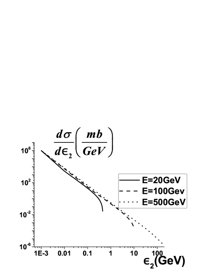
Figure 6: Born differential cross section, defined by Eq. (13), is calculated with the standard dipole fit of the form factors at different beam energies.

The sensitivity of this cross section to different form factor parameterizations is shown in Fig.7, in terms of the quantities (in percent)

$$R^{r}=1-\frac{d\,\sigma^{r}}{d\,\sigma^{sd}}\,,\ \ R^{m}=1-\frac{d\,\sigma^{m}}{d\,\sigma^{sd}}\,,\ \ R^{z}=1-\frac{d\,\sigma^{z}}{d\,\sigma^{sd}}\,,$$ (58)

where $d\,\sigma^{i}$ is the differential cross section (13), where the indices $i=r\,,~{}z\,,~{}m\,,d$ correspond to above mentioned parameterizations of the proton form factors.

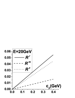
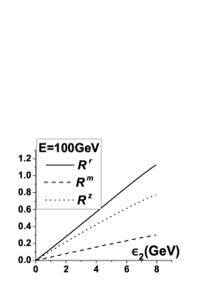
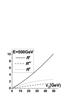
Figure 7: The difference of the recoil electron distributions (Eq. (58)) in percent for various parameterizations of the form factors, at proton energies 20 GeV, 100 GeV and 500 GeV .

The hard photon correction depends on the parameters $\Delta E_{2}$ and $\Delta\epsilon_{2},$ due to the contribution of the region 1 in Fig.4. To illustrate this dependence, we show in Fig.8 the quantities (in which the contribution of the region 2 is removed)

$$\Delta h_{E}=\frac{d\,\sigma^{(h)}(\Delta E_{2}=0.05\,E\,,~{}\Delta\epsilon_{2}=0.03\,\epsilon_{2})}{d\,\sigma^{(B)}}-\frac{d\,\sigma^{(h)}(\Delta E_{2}=0.02\,E\,,~{}\Delta\epsilon_{2}=0.03\,\epsilon_{2})}{d\,\sigma^{(B)}}\,,$$

$$\Delta h_{\epsilon}=\frac{d\,\sigma^{(h)}(\Delta E_{2}=0.02\,E\,,~{}\Delta\epsilon_{2}=0.06\,\epsilon_{2})}{d\,\sigma^{(B)}}-\frac{d\,\sigma^{(h)}(\Delta E_{2}=0.02\,E\,,~{}\Delta\epsilon_{2}=0.03\,\epsilon_{2})}{d\,\sigma^{(B)}}\,,$$ (59)

as a function of the recoil electron energy for sd-parametrization. The cross section increases with the growth of $\Delta\,E_{2}$ at fixed value $\Delta\,\epsilon_{2},$ but even decreases with the growth of $\Delta\,\epsilon_{2}$ at fixed $\Delta\,E_{2}$. Such unusual dependence on the energy-cut parameters is due to the weight function $g(\omega)$ in the integrand over the region $1$ in Fig.4. If $\Delta\,E_{2}$ increases then the region, where $g(\omega)=1,$ is enlarged. Meanwhile, the region, where $g(\omega)<1,$ is only shifted but the function $g(\omega)$ grows, and these effects lead to the enhancement of the cross section. At increasing of $\Delta\,\epsilon_{2}$ the region, where $g(\omega)=1,$ is reduced, the region, where $g(\omega)<1,$ is enlarged and $g(\omega)$ decreases. The change of the cross section in the last case depends on interplay of these factors as well on the integrand.

Qualitatively, it can be understand if we change $C_{1}(\omega)$ in the r.h.s. of Eq. (46) by its small-$\omega$ behaviour $\sim 1/\omega$ and performing analytical integration

$$\int\limits_{\omega_{s}}^{\Delta E}g(\omega)\,\frac{d\omega}{\omega}=\ln\frac{\Delta\,E_{2}}{\omega_{s}}-\frac{1}{6}\left(\frac{\Delta\,\epsilon_{2}}{\Delta\,E_{2}}\right)^{2}\,,\ \ \frac{\Delta\,\epsilon_{2}}{\Delta\,E_{2}}\ll\,1\,.$$ (60)

Thus, when parameters $\Delta\,E_{2}$ and $\Delta\,\epsilon_{2}$ grow, the logarithmic increase with $\Delta\,E_{2}$ and very weak decrease with $\Delta\,\epsilon_{2}$ take place.

Note that our choice of parameters $\Delta E_{2}$ and $\Delta\epsilon_{2}$ is taken only for illustrative goal. Really, they have to be specific for every experiment, but our approach allows to calculate with any ones.

In Fig.9 we present the quantities $\delta^{(h)}$ and $\widetilde{\delta},$ defined as

$$\delta^{(h)}=\frac{d\,\sigma^{(h)}}{d\,\sigma^{(B)}}-\frac{2\,\alpha}{\pi}\ln\frac{\omega_{s}}{\bar{\omega}}\left[\frac{\epsilon_{2}}{k_{2}}\ln\left(\frac{\epsilon_{2}+k_{2}}{m}\right)-1\right]\,,$$

$$\widetilde{\delta}=\bar{\delta}+\delta^{(\rm vac)}+\frac{2\,\alpha}{\pi}\ln\frac{\omega_{s}}{m}\left[\frac{\epsilon_{2}}{k_{2}}\ln\left(\frac{\epsilon_{2}+k_{2}}{m}\right)-1\right]\,,$$ (61)

which we call ”modified hard and soft and virtual corrections”, respectively, as well their sum $\delta_{\rm tot}=\delta^{(h)}+\widetilde{\delta}$ that is the total model-independent first order radiative correction (the last term in $\tilde{\delta}$ is $\delta_{0}(\bar{\omega}\to\omega_{s})).$ In fact

$$\delta_{\rm tot}=\delta^{(h)}+\tilde{\delta}=\delta_{0}+\bar{\delta}+\delta^{(\rm vac)}+\frac{d\sigma^{(h)}}{d\sigma^{(B)}}\,.$$

Note, that both modified corrections in Eq.(IV) are independent on the auxiliary parameter $\bar{\omega}$ but depend on the physical parameter $\omega_{s}$ and, therefore, have a physical sense.

To calculate $\sigma_{\rm tot},$ we can write the quantity $(1+\delta_{0}(\bar{\omega}\to\omega_{s}))$ using the expression (35) or its exponential form defined by (36) (with substitution $\bar{\omega}\to\omega_{s}$). But numerical estimations show that they differ very insignificantly, by a few tenth of the percent, and further we do not use the exponential form.

We see that at small values of the squared momentum transfer (small recoil-electron energy $\epsilon_{2}$) the total model-independent radiative correction is positive and it decreases (with increase of $\epsilon_{2}$), reaching zero and becoming negative. The absolute value of the radiative correction does not exceed 6$\%,$ although the strong compensation of the large (up to 40 %) positive ”modified hard” and negative ”modified soft and virtual” corrections takes place. Such behavior of the pure QED correction is similar to one derived in Ref. Kahane (1964).

If the proton form factors are determined independently with high accuracy from other experiments, the measurement of the cross section $d\,\sigma/d\,\epsilon_{2}$ can be used, in principle, to measure the model-dependent part of the radiative correction in the considered conditions. This possibility is similar to the one described in Ref. Abbiendi et al. (2016) where the authors proposed to determine the hadronic (model-dependent) contribution to the running electromagnetic coupling $\alpha(q^{2})$ by a precise measurement of the $\mu^{-}-\,e^{-}$ differential cross section, assuming that QED model-independent radiative corrections are under control.

Figure 8: The sensitivity, as the function of the recoil electron energy, (in percent) of the hard photon correction to the parameter $\Delta E_{2}$ (above) and $\Delta\epsilon_{2}$ (bottom) Eq. (IV) at proton energy of 100 GeV (left) and 500 GeV(right).

Figure 9: (Top) The modified soft and virtual ($\widetilde{\delta}$) (dashed line) and hard $(\delta^{(h)})$ (solid line) corrections (in percent) as defined by Eq.(IV). (Bottom) The total radiative correction (in percent) calculated for the standard dipole fit at $\Delta E_{2}=0.02\,E$, at 100 GeV (left) and 500 GeV (right) incident proton energy.

In Fig.10 we illustrate the sensitivity of the total radiative correction to the parametrization of the form factors in terms of the ratios

$$P^{i}=\frac{1+\delta_{\rm tot}^{i}}{1+\delta_{\rm tot}}-1\,,\ \ i=r,\,m\,,$$ (62)

where $\delta_{\rm tot}$ is the total correction for standard dipole fit. We see that, in the considered conditions, the deviation of these quantities from unity is very small and conclude that influence of the parameterizations of the form factors on the radiative correction is much smaller than this influence on the Born cross section. Moreover, the $r$ and $m$ parameterizations decrease the Born cross section relative to the $d$ one, as it follows from Fig.7, whereas for the radiative correction we have just opposite effect.

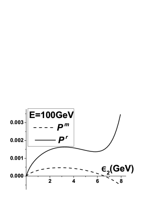
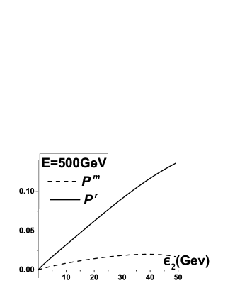
Figure 10: The sensitivity of the total model-independent radiative correction (in percent) to the choice of the form factor parametrization (Eq (62)).

V Conclusion

In present paper we investigated the recoil-electron energy distribution in elastic proton-electron scattering in coincidence experimental setup, taking the model-independent QED radiative corrections into account. The detection of the recoil electron in this process, with energies from a few MeV up to a few tens GeV, will allow to receive the small-$Q^{2}$ data, at 10^-5 GeV² $\leq Q^{2}\leq$ 3$\cdot$10^-2 GeV${}^{2}.$ Such data, being combined with the existing and planning in the future experiments with the electron beams, will help to perform more precise analysis of the small-$Q^{2}$ behavior of the proton electromagnetic form factors. It allows to obtain meaningful extrapolation to the static point and to extract the proton charge radius. As noted in the recent review Hill (2017), it is interesting to extract the proton charge radius entirely from low-$Q^{2}$ data. High precision measurements, in the inverse kinematics, allow to accumulate a lot of such data.

To cover the above mentioned interval of the $Q^{2}$-values, it is desirable to use the proton beams with large enough energies, of the order of a few hundreds GeV. At very small $Q^{2},$ the sensitivity of the differential cross section to the form factors parameterizations is practically absent, but at $Q^{2}\approx$ 2$\cdot$10^-3 GeV² it has become noticeable and reaches several percent at $Q^{2}\approx$ 3$\cdot$10^-2 GeV² (see Fig. 7). As follows from the relations (IV), the sensitivity to the value of the proton charge radius also increases essentially with the growth of the proton beam energy.

The effect, caused by the changing of the form factors parametrization in the small-$Q^{2}$ region, is rather small. Therefore, the accuracy of the measurement has to be high enough. In Ref. Vorobyev (2016), it is noted that in planning experiment at the Mainz Microtron, with detection of the recoil proton, the measurement precision has to be at the level of 0.2%. To discriminate between different form factor parameterizations the accuracy, in the inverse kinematics experiments, must be the same, possibly somewhat less with growth of $Q^{2}$ and the proton beam energy. At such conditions the radiative corrections have to be under control.

We account for the first order QED corrections caused by the vacuum polarization and the radiation of the real and virtual photons by the initial and final electrons, paying special attention to the calculation of the hard photon emission contribution when the final proton and electron energies are determined. This hard radiation takes place due to the imprecision in the measurement of the proton (electron) energy, $\Delta E\,\ (\Delta\varepsilon_{2})$. In our calculations we follow Ref.  Kahane (1964) in choice of the coordinate system and the angular integration method. We derive analytical (although very cumbersome) expressions for the functions $C_{1}(\omega)$ and $C_{2}(\omega),$ defined by Eqs.(III.3). The cancelation of the auxiliary infrared parameter $\bar{\omega}$ in the sum of the soft and hard corrections is performed analytically and the rest $\omega-$integration in (46) is done numerically.

The increase of the parameter $\Delta\epsilon_{2}$ leads to the small decrease of the hard photon correction. The magnitude of this decrease is about 0.01 (0.025) $\%$ at E=100 (500) GeV. Contrary, the increase of the parameter $\Delta E_{2}$ increases the hard photon correction by $\approx$ 0.2 (1)$\%$ at E=100 (500) GeV (see Fig. 8). Such different behaviour of this correction can be explained, on the qualitative level, by Eq. (60).

As usually, there is a strong cancellation between the positive hard correction and negative virtual and soft ones, as it is seen in Fig. 9. Despite the fact that the absolute values of these corrections separately reach 20 $-$40$\%$, their sum $|\delta_{\rm tot}|$ does not exceed 6$\%$ at E=100 GeV and 4$\%$ at E=500 GeV for the values $\Delta E_{2}=0.02\,E\,,\ \Delta\varepsilon_{2}=0.3\,\varepsilon_{2}$ used in calculations. The total correction shows the very weak dependence on the form factors parametrization (see. Fig. 10) in the considered region. At the lower values of $Q^{2},$ which correspond to the lower values of the recoil electron energy $\varepsilon_{2},$ the total correction $\delta_{\rm tot}$ is positive and changes sign when $Q^{2}$ increases. Such behaviour of $\delta_{\rm tot}$ is similar to the one found in Ref.  Kahane (1964) and confirmed in paper Bardin et al. (1969) for the case of the pion electron scattering.

In the papers Kahane (1964); Bardin et al. (1969), the authors calculated also the model-dependent part of the radiative corrections, using the point-like scalar electrodynamics to describe the interaction of the charged pion with a photon.

In our case, the effect of the model-dependent corrections, when virtual and real photons are emitted by the initial and final protons, can be roughly evaluated in the approximation of the structureless proton with the minimal proton-photon interaction ($F_{1}(q^{2})=1\,,\ F_{2}(q^{2})=0$), under the condition $Q^{2}/M^{2}\ll 1.$ The account for the proton structure can not change estimation essentially. To derive the virtual and soft corrections in this approximation, it is enough to write, in the expression ($\delta_{0}+\bar{\delta}$) defined in Eq. (35) (where $\bar{\delta}$ is taken without the term proportional to $M^{2}$), $\varepsilon_{2}$ and $k_{2}$ in terms of $Q^{2}$ and $m$, after that to change $m\to M$ and then to use the condition $Q^{2}/M^{2}\ll 1.$ Such procedure gives their sum as

$$\frac{\alpha}{\pi}\frac{Q^{2}}{M^{2}}\bigg{(}\frac{85}{36}+\frac{4}{3}\ln\frac{M^{2}}{Q^{2}}+\frac{2}{3}\ln\frac{\bar{\omega}}{M}-2\ln{2}\bigg{)}\,.$$ (63)

The largest negative term with unphysical parameter $\bar{\omega}$ has to be cancelled by the hard photon contribution. The rest terms, in (63) at $Q^{2}$=3$\cdot$10^-2 GeV², do not exceed 0.5$\cdot$10^-3 that is a few times smaller than the required measurement accuracy. In this approximation, the vertex correction modifies also the Born value of the proton anomalous magnetic moment and that leads to

$$G_{M}(q^{2})\to G_{M}(q^{2})+\frac{\alpha}{2\,\pi}\bigg{(}1+\frac{q^{2}}{6\,M^{2}}\bigg{)}\,.$$

Taking $\mu_{p}=2.793$, we evaluate that the correction to the Born value of $G_{M}^{2}$ is no more than 0.8$\cdot$10${}^{-3}.$ The up-down interference, that is part of model-dependent QED corrections, which include the two-photon exchange and the interference of the proton and electron radiation, has to be suppressed in considered kinematics at least by the factor

$$\frac{\alpha}{\pi}\,\frac{Q^{2}}{2m\,E}\,\ln\frac{2m\,E}{Q^{2}}\,,$$

that is no more than 0.1$\%.$ The analysis of the two-photon-exchange in the elastic $e^{-}$-p scattering at small-$Q^{2}$, performed in Gorchtein (2014) for the more realistic model, confirms such suppression.

Thus, we conclude that the model-independent part of the radiative corrections are under control and, if necessary, it can be calculated with a more high accuracy. We believe that the uncertainty due to the model-dependent part in the region $Q^{2}\ll M^{2}$ is small and can not affect the experimental cross sections measured even with 0.2$\%$ accuracy.

VI Acknowledgments

This work was partially supported by the Ministry of Education and Science of Ukraine (projects no. 0115U000474 and no. 0117U004866). The research is conducted in the scope of the IDEATE International Associated Laboratory (LIA).

Appendix

Since we use the expressions for the proton form factor expanded into series up to term of the order of $q_{1}^{4}$ and the function $W_{1}(q_{1}^{2})$ is proportional to $q_{1}^{2}$ we have to calculate the integrals (45) over the variables $\varphi$ and $y$ with the following integrands $S_{1}/(q_{1}^{2}\,|\vec{p}-\vec{k}|)\,,S_{1}/|\vec{p}-\vec{k}|,\\ S_{2}/(q_{1}^{4}\,|\vec{p}-\vec{k}|)\,,\ S_{2}/(q_{1}^{2}\,|\vec{p}-\vec{k}|)\,,\ S_{2}/|\vec{p}-\vec{k}|\,.$

Let us introduce the following notation for integrals

$$J_{i\beta}=\int\limits_{y_{-}}^{y_{+}}d\,y\int\limits_{0}^{2\pi}d\,\varphi\,\frac{S_{i}}{(q_{1}^{2})^{\beta}|\vec{p}-\vec{k}|},\ \ I_{i\beta}=\int\limits_{y_{-}}^{\bar{y}}d\,y\int\limits_{0}^{2\pi}d\,\varphi\,\frac{S_{i}}{(q_{1}^{2})^{\beta}|\vec{p}-\vec{k}|}\,,\ i=1,\,2,\ \beta=0,\,1,\,2;$$ (A.1)

$$\ d_{\pm}=\omega+\epsilon_{2}\pm m\,,\ k_{h}=\sqrt{d_{+}\,d_{-}}\,,\ \epsilon_{\pm}=\epsilon_{2}\pm m\,,\ \ Z=m^{2}+M^{2}+2mE\,,$$

$$E_{2}=m+E-\omega-\epsilon_{2},\,\left|\overset{\rightharpoonup}{p_{2}}\right|=\sqrt{(m+E-\omega-\epsilon_{2})^{2}-M^{2}}.$$

Then we have

$$J_{22}=\frac{2\pi}{\omega^{2}}\Big{[}C_{22}+\frac{\overline{C}_{22}}{m\omega}\,L^{(\omega)}+\frac{2\widetilde{C}_{22}}{m\,k_{h}}L^{(h)}\Big{]}\,,\$$ (A.2)

$$L^{(\omega)}=\ln\Big{(}1-\frac{2\omega\,d_{-}}{m\epsilon_{-}}\Big{)}\,,\ \ L^{(h)}=\ln\frac{\omega+\epsilon_{2}+k_{h}}{m}\,,$$

$$C_{22}=2+\frac{\epsilon_{+}[7m^{3}+2E\left(4m-3\epsilon_{2}\right)m+E^{2}\left(m-6\epsilon_{2}\right)+\left(M^{2}-m^{2}\right)\epsilon_{2}]}{2\,m^{3}\,d_{+}}-$$

$$\frac{6m^{3}\epsilon_{-}-\left(8M^{2}+\left|\overset{\rightharpoonup}{k_{2}}\right|^{2}\right)m^{2}+6E\left(4m^{2}-\epsilon_{2}\epsilon_{+}\right)m-M^{2}\epsilon_{2}\left(3m+7\epsilon_{2}\right)-E^{2}\left(\left|\overset{\rightharpoonup}{k_{2}}\right|^{2}+5\epsilon_{2}\epsilon_{+}\right)}{2\,m^{3}\,d_{-}}+$$

$$\frac{4\epsilon_{2}\,M^{2}[m\left(\epsilon_{2}-\omega\right)-2\omega\epsilon_{2}]}{m^{3}[m\omega+d_{-}(2\omega-m)]}+\frac{\left(8m^{2}-5\epsilon_{2}m-\epsilon_{2}^{2}\right)M^{2}+2mE\left(9m-2\epsilon_{2}\right)\epsilon_{-}+3E^{2}\left(4m^{2}-\epsilon_{2}\epsilon_{+}\right)}{m^{2}\,d_{-}^{2}}$$

$$-\frac{3(m+E)^{2}\epsilon_{+}^{2}}{m^{2}\,d_{+}^{2}}+\frac{2\epsilon_{-}[2Em^{2}+E^{2}\left(2\epsilon_{2}-9m\right)+M^{2}\left(2\epsilon_{2}-5m\right)]}{m\,d_{-}^{3}}-\frac{2m\epsilon_{-}(3M^{2}+2E^{2})}{d_{-}^{4}}\,,$$

$$\overline{C}_{22}=\frac{2[(\epsilon_{2}-2m)M^{2}-2mE(E+2\epsilon_{-})]}{d_{-}}-\frac{\epsilon_{-}[3M^{2}\left(\epsilon_{2}-3m\right)-2mE\left(-5m+4E+3\epsilon_{2}\right)]}{d_{-}^{2}}+$$

$$\frac{\epsilon_{-}[\left(12m^{2}-9\epsilon_{2}m+\epsilon_{2}^{2}\right)M^{2}+2mE^{2}\left(5m-3\epsilon_{2}\right)+2mE\epsilon_{-}\left(3m-\epsilon_{2}\right)]}{d_{-}^{3}}+$$

$$\frac{2m\,\epsilon_{-}^{2}[\left(M^{2}+E^{2}\right)\epsilon_{2}-m\left(4M^{2}+3E^{2}-mE\right)]}{d_{-}^{4}}-\frac{\epsilon_{-}^{2}m^{3}(3M^{2}+2E^{2})}{d_{-}^{5}}+4m\,E\,,$$

$$\widetilde{C}_{22}=\frac{\epsilon_{-}\left(5m-\epsilon_{2}\right)m^{2}+2m\,E\left(2m-\epsilon_{2}\right)\left(3m-\epsilon_{2}\right)+p^{2}\epsilon_{2}\epsilon_{+}+E^{2}\left(5m^{2}+3\epsilon_{2}^{2}\right)}{4m\,d_{-}}+$$

$$\frac{\epsilon_{+}[9m^{3}+2m\,E(6m-\epsilon_{2})+m^{2}\epsilon_{2}-3E^{2}\epsilon_{-}-p^{2}\epsilon_{2}]}{4m\,d_{+}}-\frac{3(m+E)^{2}\epsilon_{+}^{2}}{2\,d_{+}^{2}}-$$

$$\frac{10m^{2}E\epsilon_{-}+E^{2}(2m-\epsilon_{2})(3m-\epsilon_{2})+M^{2}\epsilon_{-}(2m+\epsilon_{2})}{2\,d_{-}^{2}}-\frac{5m^{2}E^{2}\epsilon_{-}}{d_{-}^{3}}-2m^{2}-2mE-M^{2}\,,$$

$$J_{21}=\frac{8\pi}{\omega^{2}}\Big{[}C_{21}+\frac{\overline{C}_{21}M^{2}}{2\omega}\,L^{(\omega)}+\frac{\widetilde{C}_{21}}{k_{h}}L^{(h)}\Big{]}\,,$$ (A.3)

$$C_{21}=\frac{2\omega^{2}(3E+2m-\omega)}{3m}-\frac{\omega(2E^{2}+2mE+m^{2})+\epsilon_{2}(M^{2}+m^{2})+2(m^{3}+m^{2}E-\epsilon_{2}E^{2})}{m}+$$

$$\frac{\epsilon_{+}[2m^{2}(7E+5m)+\epsilon_{2}(2m^{2}+M^{2})+E^{2}(4m-3\epsilon_{2})]}{2m\,d_{+}}-\frac{3(E+m)^{2}\epsilon_{+}^{2}}{d_{+}^{2}}-$$

$$\frac{\epsilon_{-}(6m^{2}E+4mM^{2}+p^{2}\epsilon_{2})-2mE^{2}\epsilon_{2}}{2m\,d_{-}}+\frac{m\epsilon_{-}(3E^{2}-M^{2})}{d_{-}^{2}}\,,$$

$$\overline{C}_{21}=-2(\omega+m-\epsilon_{2})+\frac{\epsilon_{-}(5m-3\epsilon_{2})}{d_{-}}-\frac{\epsilon_{-}^{2}(3m-\epsilon_{2})}{d_{-}^{2}}-\frac{m^{2}\,\epsilon_{-}^{2}}{d_{-}^{3}}\,,$$

$$\widetilde{C}_{21}=\omega(m^{2}+Z)+\epsilon_{2}(-3m^{2}+Z)-m[3m^{2}+2E(E+3m)]+$$

$$\frac{\epsilon_{-}\left(6Em^{2}+M^{2}\epsilon_{2}\right)+E^{2}\left(2m^{2}-5m\epsilon_{2}+\epsilon_{2}^{2}\right)}{2d_{-}}-\frac{3E^{2}m^{2}\epsilon_{-}}{d_{-}^{2}}+$$

$$+\frac{\epsilon_{+}}{2d_{+}}\big{[}2m(E+m)\left(3E+6m+2\epsilon_{2}\right)-\epsilon_{2}p^{2}\big{]}-\frac{3m(E+m)^{2}\epsilon_{+}^{2}}{d_{+}^{2}}\,.$$

$$J_{20}=\frac{16\pi}{\omega^{2}}\Big{[}C_{20}+\frac{\widetilde{C}_{20}m}{k_{h}}L^{(h)}\Big{]}\,,$$ (A.4)

$$C_{20}=-\frac{4\omega^{5}}{5\,m}+\frac{2\omega^{4}\left(20E+19m-10\epsilon_{2}\right)}{15m}-\frac{\omega^{3}}{3m}\Big{[}2\left(4E^{2}+6m^{2}+9Em\right)-8\epsilon_{2}(E+m)-M^{2}\Big{]}+$$

$$\frac{\omega^{2}}{3m}\Big{[}11m^{3}-\epsilon_{2}\left(8m^{2}+3M^{2}\right)+2m\left(5E^{2}-M^{2}\right)+2Em\left(11m-5\epsilon_{2}\right)\Big{]}+$$

$$\omega[m^{3}+2m(M^{2}-2E^{2})+\epsilon_{2}(2m^{2}+4mE+M^{2})]-\frac{E^{2}m^{2}\epsilon_{-}}{d_{-}}-\frac{6m^{2}(E+m)^{2}\epsilon_{+}^{2}}{d_{+}^{2}}+$$

$$+\frac{m\,\epsilon_{+}\left[m\left(7E^{2}+13m^{2}\right)+\epsilon_{2}\left(5m^{2}+M^{2}\right)+2Em\left(10m+3\epsilon_{2}\right)\right]}{d_{+}}\,,$$

$$\widetilde{C}_{20}=-\omega^{2}(m^{2}+Z)+\omega[m^{3}+2m(E+m)(E+2m)-2\epsilon_{2}(2mE+M^{2})]-m^{3}(E-2\epsilon_{2})-$$

$$m^{2}(4E+9m)(E+\epsilon_{+})-2mE\,\left|\overset{\rightharpoonup}{k_{2}}\right|^{2}+\epsilon_{2}M^{2}(m-2\epsilon_{2})+2m\epsilon_{2}\,E(E-\epsilon_{+})+\frac{m^{2}E^{2}\epsilon_{-}}{d_{-}}+$$

$$\frac{6m^{2}(E+m)^{2}\epsilon_{+}^{2}}{d_{+}^{2}}+\frac{m\epsilon_{+}[\epsilon_{2}(2E^{2}+10mE+7m^{2}+M^{2})+3m(E+m)(3E+5M)]}{d_{+}}\,.$$

$$J_{11}=\frac{16\pi}{\omega^{2}}\Big{[}C_{11}-\frac{\overline{C}_{11}L^{(\omega)}}{2\omega d_{-}^{3}}+\frac{\widetilde{C}_{11}}{k_{h}}L^{(h)}\Big{]}\,,$$ (A.5)

$$C_{11}=-\frac{3m^{4}-m^{3}\left(\omega+2\epsilon_{2}\right)-m^{2}\left(2\omega^{2}+5\omega\epsilon_{2}+3\epsilon_{2}^{2}\right)+2m\epsilon_{2}\left(\omega+\epsilon_{2}\right){}^{2}+\omega\left(\omega+\epsilon_{2}\right){}^{3}}{md_{-}^{2}\,d_{+}}\,,$$

$$\overline{C}_{11}=2\omega^{4}+4\omega^{3}\epsilon_{-}+\omega^{2}(5m^{2}-8m\epsilon_{2}+3\epsilon_{2}^{2})-\omega\epsilon_{-}^{2}(3m-\epsilon_{2})+m^{2}\epsilon_{-}^{2}\,,$$

$$\widetilde{C}_{11}=-\frac{3m^{2}\epsilon_{-}}{2d_{-}{}^{2}}+\frac{7m^{2}-13m\epsilon_{2}+4\epsilon_{2}^{2}}{4d_{-}}-\frac{3m\epsilon_{+}}{4d_{+}}+d_{+}\,.$$

$$J_{10}=\frac{16\pi}{\omega^{2}}\Big{[}C_{10}-\frac{m\,\widetilde{C}_{10}}{k_{h}^{3}}L^{(h)}\Big{]}\,,$$ (A.6)

$$C_{10}=-m^{2}\big{[}\frac{\epsilon_{-}}{d_{-}}+\frac{3\epsilon_{+}}{d_{+}}\big{]}-\frac{2\omega^{2}(d_{+}+2\epsilon_{2})}{3\,m}+2\omega\epsilon_{+}+4m\epsilon_{-}\,,$$

$$\widetilde{C}_{10}=(\epsilon_{2}+\omega)^{2}\,[2\,\left|\overset{\rightharpoonup}{k_{2}}\right|^{2}+m(\omega-4\epsilon_{2})+\omega^{2}+2\omega\epsilon_{2}]+m^{2}[\omega\epsilon_{+}+4m\,\epsilon_{2}]\,.$$

$$I_{22}=\frac{2\pi}{\omega^{2}}\Big{[}D_{22}+\frac{D_{22}^{L_{1}}}{m\,k_{h}}L_{1}+\frac{D_{22}^{L_{2}}}{m\,\omega}L_{2}+\frac{1}{m\omega K_{2}}D_{22}^{2}+\frac{\omega K_{1}}{m^{2}k_{h}\,d_{-}}\overline{D}_{22}^{1}+\frac{K_{2}}{m^{2}\omega\,d_{-}^{3}}\overline{D}_{22}^{2}+$$

$$\frac{1}{m\omega(2mp^{2}-d_{-}Z)}\Big{(}\frac{2mE^{2}-d_{-}(M^{2}+2mE)}{k_{h}\,K_{1}}D_{22}^{1}+p\,D_{22}^{p}\Big{)}\Big{]}\,,$$ (A.7)

$$K_{1}=\sqrt{\frac{m^{2}(2mp^{2}-d_{-}Z)}{d_{+}^{2}\,d_{-}}+\frac{1}{\omega^{2}}\big{(}\left|\overset{\rightharpoonup}{k_{2}}\right|\left|\overset{\rightharpoonup}{p_{2}}\right|-\frac{(E_{2}-m)(\left|\overset{\rightharpoonup}{k_{2}}\right|^{2}+\omega\epsilon_{2})}{d_{+}}\Big{)}^{2}}\,,$$

$$K_{2}=\sqrt{\big{(}\left|\overset{\rightharpoonup}{k_{2}}\right|\left|\overset{\rightharpoonup}{p_{2}}\right|d_{-}-\epsilon_{-}(\epsilon_{2}+\omega)E_{2}\big{)}^{2}+m\epsilon_{-}M^{2}(2\omega d_{-}-m\epsilon_{-})}\,,$$

$$L_{1}=\ln\frac{\omega k_{h}^{2}K_{1}+d_{-}[\left|\overset{\rightharpoonup}{k_{2}}\right|\left|\overset{\rightharpoonup}{p_{2}}\right|d_{+}-(E_{2}-m)(\left|\overset{\rightharpoonup}{k_{2}}\right|^{2}+\omega\epsilon_{2})]}{\omega(\omega+\epsilon_{2}-k_{h})[pk_{h}+(E+m)d_{-}]}\,,$$

$$L_{2}=\ln\frac{K_{2}+\epsilon_{-}E_{2}(\omega+\epsilon_{2})-\left|\overset{\rightharpoonup}{k_{2}}\right|\left|\overset{\rightharpoonup}{p_{2}}\right|d_{-}}{m\epsilon_{-}(E+p)}\,,$$

$$D_{22}=1+\frac{2\epsilon_{2}M^{2}(m(\epsilon_{2}-\omega)-2\omega\epsilon_{2})}{m^{3}(2\omega d_{-}-m\epsilon_{-})}+\frac{\epsilon_{+}}{4m^{3}d_{+}}\Big{[}E^{2}(m-6\epsilon_{2})+2mE(4m-3\epsilon_{2})+\epsilon_{2}(M^{2}-m^{2})+7m^{3}\Big{]}-$$

$$\frac{1}{4m^{3}d_{-}}\big{[}\epsilon_{+}E^{2}(m-6\epsilon_{2})+6mE(4m^{2}-\epsilon_{2}\epsilon_{+})-\epsilon_{2}M^{2}(3m+7\epsilon_{2})-m^{2}(8M^{2}+\epsilon_{2}^{2})+m^{3}(6\epsilon_{2}-5m)\big{]}-$$

$$\frac{3\epsilon_{+}^{2}(E+m)^{2}}{2m^{2}d_{+}^{2}}+\frac{1}{2m^{2}d_{-}^{2}}\big{[}3E^{2}(4m^{2}-\epsilon_{2}\epsilon_{+})+2m\epsilon_{-}E(9m-2\epsilon_{2})+M^{2}(8m^{2}-5m\epsilon_{2}-\epsilon_{2}^{2})\big{]}+$$

$$\frac{\epsilon_{-}}{md_{-}^{3}}\big{[}E^{2}(2\epsilon_{2}-9m)+2m^{2}E+M^{2}(2\epsilon_{2}-5m)\big{]}-\frac{m\epsilon_{-}(3M^{2}+2E^{2})}{d_{-}^{4}}\,,$$

$$D_{22}^{L_{1}}=-2m(E+m)-M^{2}+\frac{\epsilon_{+}}{4md_{+}}[9m^{3}+2m\,E(6m-\epsilon_{2})+\epsilon_{2}(m^{2}-p^{2})-3\epsilon_{-}E^{2}]+\frac{1}{4md_{-}}[p^{2}\epsilon_{2}\epsilon_{+}\,+$$

$$12m^{3}E+E^{2}(5m^{2}+3\epsilon_{2}^{2})+m(5m-\epsilon_{2})(m\epsilon_{-}-2\epsilon_{2}E)]-\frac{3\epsilon_{+}^{2}(E+m)^{2}}{2d_{+}^{2}}+$$

$$\frac{1}{2d_{-}^{2}}[-m\epsilon_{-}(10mE+M^{2})-M^{2}\left|\overset{\rightharpoonup}{k_{2}}\right|^{2}-E^{2}(6m^{2}-5m\epsilon_{2}+\epsilon_{2}^{2})]+\frac{5m^{2}E^{2}\epsilon_{-}}{d_{-}^{3}}\,,$$

$$D_{22}^{L_{2}}=4mE+\frac{2}{d_{-}}[\epsilon_{2}M^{2}-4m\epsilon_{-}E-2m(E^{2}+M^{2})]+\frac{\epsilon_{-}}{d_{-}^{2}}[2mE(4E+3\epsilon_{2}-5m)-3M^{2}(\epsilon_{2}-3m)]+$$

$$\frac{\epsilon_{-}}{d_{-}^{3}}[M^{2}(12m^{2}-9m\epsilon_{2}+\epsilon_{2}^{2})+2mE^{2}(5m-3\epsilon_{2})+2m\epsilon_{-}E(3m-\epsilon_{2})]+$$

$$\frac{2m\epsilon_{-}^{2}}{d_{-}^{4}}[m^{2}E+M^{2}(\epsilon_{2}-4m)+E^{2}(\epsilon_{2}-3m)]-\frac{m^{3}\epsilon_{-}^{2}(3M^{2}+2E^{2})}{d_{-}^{5}}\,,$$

$$\overline{D}_{22}^{1}=\left|\overset{\rightharpoonup}{k_{2}}\right|\left|\overset{\rightharpoonup}{p_{2}}\right|+3m^{2}+\epsilon_{2}(d_{+}-E)-\frac{3m\epsilon_{+}(m+E)}{d_{+}}-\frac{4m^{2}E}{d_{-}}\,,\ \ \overline{D}_{22}^{2}=\omega^{2}\epsilon_{+}+\omega[\left|\overset{\rightharpoonup}{k_{2}}\right|\left|\overset{\rightharpoonup}{p_{2}}\right|+\epsilon_{2}^{2}-$$

$$\epsilon_{2}(m+E)-3mE]+m[m(2m-7E)+\epsilon_{2}(3E-2m)]+\frac{\epsilon_{-}mE(7m-3\epsilon_{2})}{d_{-}}\,,$$

$$D_{22}^{1}=\left|\overset{\rightharpoonup}{k_{2}}\right|^{2}\,Z+m^{2}\epsilon_{2}(E+m)+\frac{1}{8d_{-}}\big{\{}4\left|\overset{\rightharpoonup}{k_{2}}\right|\left|\overset{\rightharpoonup}{p_{2}}\right|[2\epsilon_{2}(M^{2}+mE)+\epsilon_{+}(m^{2}-E^{2})]-$$

$$\epsilon_{+}E^{3}(3m-5\epsilon_{2})-mE^{2}[6m\epsilon_{2}-5(5m^{2}-3\epsilon_{2})]+\epsilon_{+}E[4m^{2}\epsilon_{-}-M^{2}(9\epsilon_{2}-7m)]-$$

$$m[8m^{3}\epsilon_{-}-\epsilon_{+}M^{2}(17m-15\epsilon_{2})]\big{\}}+\frac{\epsilon_{+}(E+m)}{8d_{+}}\big{[}4\left|\overset{\rightharpoonup}{k_{2}}\right|\left|\overset{\rightharpoonup}{p_{2}}\right|(E+m)-8m^{2}\epsilon_{2}+$$

$$4mE(m-3\epsilon_{2})+E^{2}(3m-5\epsilon_{2})+\epsilon_{+}M^{2}\big{]}+\frac{1}{4d_{-}^{2}}\big{\{}4m\left|\overset{\rightharpoonup}{k_{2}}\right|\left|\overset{\rightharpoonup}{p_{2}}\right|[\epsilon_{-}(M^{2}+mE)-\epsilon_{2}p^{2}]+$$

$$m\epsilon_{-}[p^{2}E(5m+3\epsilon_{2})-mE^{2}(7m+\epsilon_{2})+4m^{2}E\epsilon_{-}+mM^{2}(3m+5\epsilon_{2})]\big{\}}-\frac{m^{2}p^{2}\epsilon_{-}}{2d_{-}^{3}}[2\left|\overset{\rightharpoonup}{k_{2}}\right|\left|\overset{\rightharpoonup}{p_{2}}\right|+\epsilon_{-}(E+m)]\,,$$

$$D_{22}^{2}=\left|\overset{\rightharpoonup}{k_{2}}\right|\left|\overset{\rightharpoonup}{p_{2}}\right|\Big{[}d_{-}[2m(E+2\epsilon_{-})-M^{2}]-2mE^{2}+3\epsilon_{-}(2m^{2}-4mE+M^{2})-\epsilon_{2}\,M^{2}\Big{]}+$$

$$\omega^{2}[2m\epsilon_{-}(E+2\epsilon_{2})-M^{2}\epsilon_{+}]+\frac{5m^{4}\epsilon_{-}^{3}p^{2}E}{d_{-}^{5}}+$$

$$\omega\big{[}mE(M^{2}-4\epsilon_{-}E)-2m\epsilon_{2}^{2}(5m+6E-4\epsilon_{2})-2m^{3}(E-3m)+\epsilon_{2}[E(14m^{2}+M^{2})-4m^{3}]\big{]}+\frac{\epsilon_{-}}{2}\big{[}2m^{2}(5M^{2}-$$

$$8E^{2})+2mE(25m^{2}-3M^{2}+2E^{2})+2\epsilon_{2}E(16mE-18m^{2}-7m\epsilon_{2}-M^{2})+\epsilon_{2}\epsilon_{-}(8m\epsilon_{2}-M^{2})\big{]}-$$

$$\frac{\epsilon_{2}M^{2}}{2m(2\omega d_{-}-m\epsilon_{-})}\big{\{}\left|\overset{\rightharpoonup}{k_{2}}\right|^{2}[2E(2\omega\epsilon_{2}-md_{-})-m\epsilon_{-}(m-2\omega)]+2\left|\overset{\rightharpoonup}{k_{2}}\right|\left|\overset{\rightharpoonup}{p_{2}}\right|\epsilon_{-}[m\omega-\epsilon_{2}(m-2\omega)]\big{\}}+$$

$$\frac{\epsilon_{-}}{md_{-}}\big{\{}\left|\overset{\rightharpoonup}{k_{2}}\right|\left|\overset{\rightharpoonup}{p_{2}}\right|[2m^{2}(3M^{2}+4E^{2})+m^{2}E(7\epsilon_{2}-23m)-\epsilon_{-}(2m^{3}-\epsilon_{2}M^{2})]+2m^{2}p^{2}[\epsilon_{-}(20m-7\epsilon_{2})+$$

$$E(3m-4\epsilon_{2})]+E[2m^{3}(17m^{2}-3M^{2})-m^{2}\epsilon_{2}(57m^{2}+5M^{2})+\epsilon_{2}^{2}\big{(}2m(12m^{2}+M^{2})+\epsilon_{2}(M^{2}-m^{2})\big{)}]+$$

$$m\epsilon_{-}[M^{2}(30m^{2}-17m\epsilon_{2}+\epsilon_{2}^{2})-3m^{3}\epsilon_{-}]\big{\}}+\frac{\epsilon_{-}}{d_{-}^{2}}\big{\{}\left|\overset{\rightharpoonup}{k_{2}}\right|\left|\overset{\rightharpoonup}{p_{2}}\right|m\big{[}E^{2}(17m-7\epsilon_{2})+2M^{2}(4m-3\epsilon_{2})-$$

$$\epsilon_{-}\big{(}m^{2}+E(\epsilon_{2}-17m)\big{)}\big{]}-\epsilon_{-}\big{[}mE^{3}(17m-7\epsilon_{2})-2mE^{2}(25m^{2}-20m\epsilon_{2}+\epsilon_{2}^{2})+E\big{(}m^{2}(22m^{2}-23m\epsilon_{2}+$$

$$\epsilon_{2}-23M^{2})+M^{2}\epsilon_{2}(2m+\epsilon_{2})\big{)}+m^{2}(m^{2}\epsilon_{-}+9mM^{2}+\epsilon_{2}M^{2})\big{]}\big{\}}+\frac{m\epsilon_{-}^{2}}{d_{-}^{3}}\big{\{}\left|\overset{\rightharpoonup}{k_{2}}\right|\left|\overset{\rightharpoonup}{p_{2}}\right|[E^{2}(\epsilon_{2}-15m)+$$

$$8m^{2}E+M^{2}(\epsilon_{2}-7m)]-mE^{3}(22m-19\epsilon_{2})-\epsilon_{2}^{2}p^{2}E-mE[M^{2}(14\epsilon_{2}-27m)-7m^{2}\epsilon_{-}]+$$

$$m\epsilon_{-}[3mM^{2}+E^{2}(2\epsilon_{2}-35m)]\big{\}}-\frac{m^{2}\epsilon_{-}^{2}}{d_{-}^{4}}\big{\{}m\left|\overset{\rightharpoonup}{k_{2}}\right|\left|\overset{\rightharpoonup}{p_{2}}\right|(7E^{2}+3M^{2})+\epsilon_{-}[m^{2}(11E^{2}-M^{2})-p^{2}E(16m-\epsilon_{2})]\big{\}}\,,$$

$$D_{22}^{p}=-2\,Z[\omega(2m-\epsilon_{2})+\epsilon_{2}^{2}]-11m^{4}+18m^{2}p^{2}+5mE(M^{2}-3m^{2})+2\epsilon_{2}[M^{2}(6m-E)+$$

$$m(4m^{2}+7mE-4E^{2})]+\frac{\epsilon_{+}^{2}(m+E)}{4md_{+}}\big{[}E^{2}(7m-6\epsilon_{2})+2mE(12m-\epsilon_{2})+m(15m^{2}+2M^{2})+\epsilon_{2}(m^{2}+3M^{2})\big{]}-$$

$$\frac{1}{4md_{-}}\big{\{}E^{3}[m^{2}(47m-8\epsilon_{2})-\epsilon_{2}^{2}(5m+6\epsilon_{2})]-mE^{2}[m^{2}(241m-302\epsilon_{2})+\epsilon_{2}^{2}(49m+8\epsilon_{2})]+E[m^{4}(75m-$$

$$167\epsilon_{2})+m^{3}(109\epsilon_{2}^{2}-118M^{2})+m^{2}\epsilon_{2}(91M^{2}-17\epsilon_{2}^{2})+\epsilon_{2}^{2}M^{2}(3\epsilon_{2}-8m)]-m\epsilon_{-}[m^{3}(79m-54\epsilon_{2})+$$

$$7m^{2}(26M^{2}+\epsilon_{2}^{2})+\epsilon_{2}M^{2}(5\epsilon_{2}-79m)]\big{\}}-\frac{3\epsilon_{+}^{3}(E+m)^{3}}{2d_{+}^{2}}+\frac{\epsilon_{-}}{2d_{-}^{2}}\big{\{}E^{3}[5m(14m-3\epsilon_{2})-3\epsilon_{2}^{2}]+$$

$$mE^{2}[m(123\epsilon_{2}-184m)-15\epsilon_{2}^{2}]-E[2m^{3}(3m+13\epsilon_{2})+8m^{2}(16M^{2}-\epsilon_{2}^{2})+\epsilon_{2}M^{2}(\epsilon_{2}-49m)]+$$

$$m[2m^{3}(13m-16\epsilon_{2})+2m^{2}(52M^{2}+3\epsilon_{2}^{2})+\epsilon_{2}M^{2}(13\epsilon_{2}-85m)]\big{\}}+\frac{m\epsilon_{-}}{d_{-}^{3}}\big{\{}E^{3}[4\epsilon_{2}^{2}+5m(11m-7\epsilon_{2})]+$$

$$mE^{2}(-61m^{2}+75m\epsilon_{2}-14\epsilon_{2}^{2})-2E[m^{3}(5m-7\epsilon_{2})+m^{2}(37M^{2}+2\epsilon_{2}^{2})+\epsilon_{2}M^{2}(4\epsilon_{2}-29m)]-$$

$$2m\epsilon_{-}[2m^{3}+3M^{2}(5m-\epsilon_{2})]\big{\}}+\frac{m^{2}\epsilon_{-}^{2}}{d_{-}^{4}}\big{\{}E^{3}(8\epsilon_{2}-36m)+18m^{2}E^{2}+E[5m^{3}+M^{2}(41m-8\epsilon_{2})]-8m^{2}M^{2}\big{\}}-$$

$$-\frac{10m^{4}\epsilon_{-}^{2}p^{2}E}{d_{-}^{5}}\,,$$

$$I_{21}=\frac{4\pi}{\omega^{2}}\Big{\{}D_{21}+\frac{D_{21}^{L_{1}}}{k_{h}}L_{1}+\frac{M^{2}\,D_{21}^{L_{2}}}{\omega}L_{2}-\frac{\omega\,K_{1}}{m\,k_{h}}\overline{D}_{21}^{1}+\frac{\overline{D}_{21}^{2}}{\omega\,d_{-}^{2}}K_{2}+$$

$$\frac{1}{2mp^{2}-d_{-}Z}\Big{[}\frac{2mEE_{2}-M^{2}d_{-}}{k_{h}\,K_{1}}D_{21}^{1}+\frac{p}{3m\,\omega}D_{21}^{p}\Big{]}\Big{\}}\,,$$ (A.8)

$$D_{21}=-\frac{2\omega^{3}}{3m}+\frac{2\omega^{2}(3E+2m)}{3m}-\frac{\omega[m^{2}+2E(m+E)]}{m}-2m(m+E)+\frac{\epsilon_{2}(E^{2}+p^{2}-m^{2})}{m}+$$

$$\frac{\epsilon_{+}}{2md_{+}}\big{[}2m^{2}(5m+7E)+E^{2}(4m-3\epsilon_{2})+\epsilon_{2}(2m^{2}+M^{2})\big{]}-\frac{1}{2m\,d_{-}}\big{\{}\epsilon_{-}[p^{2}\epsilon_{2}-2m(E^{2}-2M^{2}-3mE)]-$$

$$2m^{2}E^{2}\big{\}}-\frac{3\epsilon_{+}^{2}(m+E)^{2}}{d_{+}^{2}}+\frac{m\epsilon_{-}(3E^{2}-M^{2})}{d_{-}^{2}}+\frac{k_{2}+p_{2}}{3m\omega}\Big{\{}2\omega^{2}[-\omega+\epsilon_{-}+2(m+E)]+$$

$$\omega[p^{2}-3E^{2}+2\left|\overset{\rightharpoonup}{k_{2}}\right|\left|\overset{\rightharpoonup}{p_{2}}\right|+2\epsilon_{-}(\epsilon_{2}-E)-2m(E-\epsilon_{-})]+m[p^{2}-3E(2m+E)+2\left|\overset{\rightharpoonup}{k_{2}}\right|\left|\overset{\rightharpoonup}{p_{2}}\right|+2\epsilon_{-}(\epsilon_{2}-E)]\Big{\}}\,,$$

$$D_{21}^{L_{1}}=(\omega+\epsilon_{2})(M^{2}+2mE)-m[3m^{2}+2E(3m+E)]-2m^{2}(\epsilon_{2}-\omega)-\frac{3m^{2}\epsilon_{-}E^{2}}{d_{-}^{2}}-\frac{3m\epsilon_{+}^{2}(m+E)^{2}}{d_{+}^{2}}+$$

$$\frac{1}{2d_{-}}\big{[}\epsilon_{-}(6m^{2}E+\epsilon_{2}M^{2})+E^{2}(\epsilon_{2}^{2}+2m^{2}-5m\epsilon_{2})\big{]}+$$

$$\frac{\epsilon_{+}}{2d_{+}}\big{[}E^{2}(6m-\epsilon_{2})+2mE(9m+2\epsilon_{2})+\epsilon_{2}(4m^{2}+M^{2})+12m^{3}\big{]}\,,$$

$$D_{21}^{L_{2}}=-2(\omega-\epsilon_{-})+\frac{\epsilon_{-}(5m-3\epsilon_{2})}{d_{-}}-\frac{\epsilon_{-}^{2}(3m-\epsilon_{2})}{d_{-}^{2}}-\frac{m^{2}\epsilon_{-}^{2}}{d_{-}^{3}}\,,$$

$$\overline{D}_{21}^{1}=\left|\overset{\rightharpoonup}{k_{2}}\right|\left|\overset{\rightharpoonup}{p_{2}}\right|+\epsilon_{2}(\omega+\epsilon_{2}-E)+m(3m+\epsilon_{2})-\frac{3m\epsilon_{+}(m+E)}{d_{+}}-\frac{4m^{2}E}{d_{-}}\,,$$

$$\overline{D}_{21}^{2}=\left|\overset{\rightharpoonup}{k_{2}}\right|\left|\overset{\rightharpoonup}{p_{2}}\right|+\epsilon_{-}(\omega+\epsilon_{2}-E)-\frac{m\epsilon_{-}E}{d_{-}}\,,$$

$$D_{21}^{1}=-\frac{\left|\overset{\rightharpoonup}{k_{2}}\right|\left|\overset{\rightharpoonup}{p_{2}}\right|-\epsilon_{-}(E_{2}-m)}{\omega}\Big{\{}\epsilon_{2}(m^{2}+M^{2})+m[m(E+m)+2\epsilon_{2}E]-\frac{m\epsilon_{+}(m+E)^{2}}{d_{+}}-$$

$$\frac{m[\epsilon_{2}p^{2}-\epsilon_{-}(M^{2}+mE)]}{d_{-}}-\frac{m^{2}p^{2}\epsilon_{-}}{d_{-}^{2}}\Big{\}}-m[\epsilon_{-}(M^{2}+mE)+m\epsilon_{2}(m+E)]-$$

$$\frac{m\big{[}M^{2}[3m(E-3m)+\epsilon_{2}(7m-5E)]+E^{2}[m(13m-11\epsilon_{2})+\epsilon_{+}E]\big{]}}{4d_{-}}+$$

$$\frac{m\epsilon_{+}(m+E)[p^{2}+4m(m+E)]}{4d_{+}}-\frac{m^{2}\epsilon_{-}p^{2}(3E-m)}{2d_{-}^{2}}\,,$$

$$D_{21}^{p}=-\omega^{2}\,Z(2E^{2}-6\epsilon_{2}E+M^{2}+6m^{2})+\omega\big{\{}2p^{2}[8m^{3}+2mE(E-4\epsilon_{2})-\epsilon_{-}(m^{2}+M^{2})]+$$

$$3m^{4}(3m+2\epsilon_{2})+3mE[m^{2}(5m+4\epsilon_{2})+M^{2}(m-2\epsilon_{2})]+3M^{2}[m^{2}(4m+\epsilon_{2})-\epsilon_{2}M^{2}]\big{\}}-mp^{2}\big{\{}-4mE^{2}+$$

$$2E[m^{2}+2\epsilon_{2}(4m-3\epsilon_{2})]+2[2m(m^{2}-M^{2})+\epsilon_{2}(31m^{2}+M^{2})]\big{\}}-3m\big{\{}2m^{4}(3m+4\epsilon_{2})+m^{3}(5M^{2}+2\epsilon_{2}^{2})-$$

$$mM^{2}(M^{2}-2\epsilon_{2}^{2})+mE[2m^{2}(7m+10\epsilon_{2})+4m\epsilon_{2}^{2}-M^{2}(m-8\epsilon_{2})]+\epsilon_{2}M^{2}(20m^{2}+M^{2})\big{\}}+$$

$$\frac{3m\epsilon_{-}}{2d_{-}}\big{\{}E^{3}(10m^{2}+7m\epsilon_{2}-5\epsilon_{2}^{2})-mE^{2}[\epsilon_{2}^{2}+3m(4m-3\epsilon_{2})]+E[\epsilon_{-}(5\epsilon_{2}M^{2}-2m^{3})-$$

$$8m^{2}M^{2}]-m\epsilon_{-}M^{2}(6m-\epsilon_{2})\big{\}}+\frac{3m\epsilon_{+}^{2}(m+E)}{2d_{+}}\big{[}E^{2}(10m-3\epsilon_{2})+2mE(15m+2\epsilon_{2})+$$

$$M^{2}(2m+3\epsilon_{2})+2m^{2}(9m+2\epsilon_{2})\big{]}-\frac{3m^{3}\epsilon_{-}^{2}E}{d_{-}^{2}}[m^{2}+M^{2}+E(m+E)]-\frac{9m^{2}\epsilon_{+}^{3}(m+E)^{3}}{d_{+}^{2}}+\frac{6m^{4}\epsilon_{-}^{2}p^{2}E}{d_{-}^{3}}\,.$$

$$I_{20}=\frac{2\pi}{\omega}\Big{\{}-\frac{4}{15m}D_{20}+\frac{4m\,L_{1}}{k_{h}}D_{20}^{L_{1}}+\frac{4\omega\,k_{h}\,K_{1}}{d_{+}}\overline{D}_{20}^{1}-\frac{4\,p}{15m\,\omega}\overline{D}_{20}^{p}+\frac{\bigl{|}\overset{\rightharpoonup}{k_{2}}\bigr{|}+\bigl{|}\overset{\rightharpoonup}{p_{2}}\bigr{|}}{15\,m\,\omega}\widetilde{D}_{20}-$$

$$-\frac{4\,m}{\omega(2mp^{2}-d_{-}Z)}\Big{[}\frac{2mEE_{2}-M^{2}d_{-}}{k_{h}\,K_{1}}D_{20}^{1}+\frac{p}{2}D_{20}^{p}\Big{]}\Big{\}}$$ (A.9)

$$D_{20}=12\omega^{5}-2\omega^{4}(20E-19m-10\epsilon_{2})+5\omega^{3}[8E^{2}+12m^{2}+18mE-8\epsilon_{2}(m+E)-M^{2}]-$$

$$-5\omega^{2}[11m^{2}(m+2E)+10mE(E-\epsilon_{2})-M^{2}(2m+3\epsilon_{2})-8m^{2}\epsilon_{2}]-$$

$$15m\omega[\epsilon_{2}(M^{2}+2m^{2}+4mE)-m(4E^{2}-m^{2}-2M^{2})]+$$

$$15m^{2}[m(4E^{2}+7m^{2}+12mE+2M^{2})+\epsilon_{2}(5m^{2}+2mE-M^{2})]+\frac{15m^{3}\epsilon_{-}E^{2}}{d_{-}}+$$

$$\frac{90m^{3}\epsilon_{+}^{2}(m+E)^{2}}{d_{+}^{2}}-\frac{15m^{2}\epsilon_{+}}{d_{+}}\big{[}m(7E^{2}+13m^{2}+20mE)+\epsilon_{2}(5m^{2}+6mE+M^{2})\big{]}\,,$$

$$\overline{D}_{20}^{1}=\left|\overset{\rightharpoonup}{k_{2}}\right|\left|\overset{\rightharpoonup}{p_{2}}\right|+4m^{2}\Big{(}1-\frac{E}{d_{-}}\Big{)}-\frac{3m\epsilon_{+}(E+m)}{d_{+}}+\overset{\rightharpoonup}{k_{2}}{}^{2}+\epsilon_{2}(-E+m+\omega)\,,$$

$$D_{20}^{L_{1}}=-\omega^{2}[2m(E+m)+M^{2}]+\omega[5m^{3}+2Em\left(E+3m-2\epsilon_{2}\right)-2M^{2}\epsilon_{2}]-m^{3}\left(9m+7\epsilon_{2}\right)+$$

$$M^{2}\epsilon_{2}\left(m-2\epsilon_{2}\right)++2E^{2}m\left(\epsilon_{2}-2m\right)-2Em\left(3m\left(2m+\epsilon_{2}\right)+2\epsilon_{2}^{2}\right)+\frac{E^{2}m^{2}\epsilon_{-}}{d_{-}}-$$

$$-\frac{6m^{2}\epsilon_{+}^{2}(E+m)^{2}}{d_{+}^{2}}+\frac{m\epsilon_{+}}{d_{+}}[15m^{3}+\epsilon_{2}\left(7m^{2}+M^{2}\right)+7Em(E+2m)+2E\epsilon_{+}(E+5m)]\,,$$

$$D_{20}^{p}=4m^{2}E^{2}\left(9m^{2}+8\epsilon_{2}m+9\epsilon_{2}^{2}\right)+mE[\left(63m^{2}+17M^{2}\right)m^{2}+4\left(33m^{2}+4M^{2}\right)\epsilon_{2}m+$$

$$2\epsilon_{2}^{2}\left(51m^{2}+10\epsilon_{2}m+9M^{2}\right)]-m^{2}M^{4}+m^{4}(18m^{2}+29M^{2})+14m^{3}\epsilon_{2}\left(3m^{2}+5M^{2}\right)+$$

$$+2m\epsilon_{2}^{2}[\left(13m+2\epsilon_{2}\right)m^{2}+2M^{2}\left(15m+4\epsilon_{2}\right)]-Z\Big{\{}2m[\left(11m+29\epsilon_{2}\right)m^{2}+\epsilon_{2}^{2}\left(21m+5\epsilon_{2}\right)]+$$

$$+2mE[8m\epsilon_{2}+9\left(m^{2}+\epsilon_{2}^{2}\right)]+\frac{m\epsilon_{-}^{2}\,M^{2}(E-m)}{p^{2}}\Big{\}}+\frac{\epsilon_{+}^{2}(m^{2}-M^{2})}{m+E}\big{[}3\epsilon_{+}(m^{2}-M^{2})+Z(2m+3\epsilon_{2})\big{]}+$$

$$\frac{m^{2}(m^{2}-M^{2})^{2}}{2Z}\Big{[}\frac{(m^{2}-M^{2})^{2}}{Z}+M^{2}-m^{2}-4m\epsilon_{2}\Big{]}\,,$$

$$\overline{D}_{20}^{p}=-\frac{15m^{5}(m^{2}-M^{2})^{2}}{2Z^{2}}+\frac{15m^{5}[m^{2}-2m(\omega-\epsilon_{2})-3M^{2}]}{2Z}-\frac{15m^{3}\epsilon_{+}^{2}}{2d_{+}(m+E)}\big{(}18m^{2}+30Em+$$

$$4\epsilon_{2}m-M^{2}+13E^{2}+4E\epsilon_{2}\big{)}+15m^{3}[6m^{2}+7m\epsilon_{2}+2\epsilon_{2}^{2}+E(m+6\epsilon_{2})]+10m^{2}\epsilon_{-}M^{2}-40m^{2}\epsilon_{2}E^{2}+$$

$$5m\epsilon_{-}M^{2}E-20d_{-}E^{3}(m+\omega)+2mp^{2}(4E^{2}+M^{2})+5\omega^{2}(M^{2}E-2mE^{2}+8\epsilon_{2}E^{2}+6m^{3}-mM^{2}-$$

$$2\epsilon_{2}M^{2})+\omega\big{[}15m^{2}(4\epsilon_{2}E-3mE-2E^{2}-2m\epsilon_{+})+2p^{2}(4E^{2}+M^{2})+5M^{2}(3m^{2}+\epsilon_{2}(m+E))+$$

$$10m\epsilon_{2}E^{2}\big{]}+10m^{3}E^{2}+\frac{45m^{3}\epsilon_{+}^{3}(m+E)}{d_{+}^{2}}-\frac{15m^{3}\epsilon_{+}^{2}}{2d_{+}(m+E)}\big{(}18m^{2}+30mE+4m\epsilon_{2}-M^{2}+13E^{2}+4\epsilon_{2}E\big{)}-$$

$$\frac{15m^{3}\epsilon_{-}^{2}E}{2p^{2}d_{-}}(5E^{2}-4M^{2}-mE)\,,$$

$$\widetilde{D}_{20}=-\frac{15\left(\left|\overset{\rightharpoonup}{k_{2}}\right|-\left|\overset{\rightharpoonup}{p_{2}}\right|\right){}^{2}\big{(}\omega^{2}-p^{2}\big{)}\big{[}2E\left(m^{2}-\omega^{2}\right)+E^{2}(m+\omega)+\omega^{2}(\omega-m)\big{]}}{-2d_{-}(E+m)+p^{2}+\omega\left(\omega+2\epsilon_{2}\right)}+$$

$$-12(m+\omega)\left(\left|\overset{\rightharpoonup}{k_{2}}\right|\left|\overset{\rightharpoonup}{p_{2}}\right|+\epsilon_{-}\left(-E+\omega+\epsilon_{2}\right)\right){}^{2}+2\left(\left|\overset{\rightharpoonup}{k_{2}}\right|\left|\overset{\rightharpoonup}{p_{2}}\right|+\epsilon_{-}\left(-E+\omega+\epsilon_{2}\right)\right)\big{[}10m^{2}(E-\epsilon_{-})+$$

$$10\omega(\omega+\epsilon_{2})(\omega-2m)-10\omega^{2}(m+E)+(m+\omega)(10\epsilon_{+}E-4M^{2}-(E-\omega)^{2})\big{]}-$$

$$-130d_{-}m^{2}\omega^{2}+M^{2}\big{\{}10\big{[}-3m^{2}\left(-E+3m+\epsilon_{2}\right)+E\omega(m-2\omega)-3E\epsilon_{2}(m+\omega)+4m\omega\epsilon_{-}+\omega^{2}\epsilon_{2}\big{]}+$$

$$+\omega^{2}(13m-37\omega)\big{\}}+2p^{2}\big{\{}10[E\left(m^{2}-\omega^{2}\right)+m\epsilon_{2}(\omega-m)]-25[(m+\omega)(m^{2}+m\left(\omega+\epsilon_{2}\right)+$$

$$\epsilon_{2}(E-\omega))+\omega^{2}(\omega-2m)]+\omega(E+\omega)(m+\omega)\big{\}}$$

$$+2E\big{\{}10m^{2}[\omega\left(2\left(m+5\epsilon_{2}\right)+13\omega\right)+3m\epsilon_{-}]+\omega^{2}[\omega\left(41\omega+25\epsilon_{2}\right)-m\left(89\omega+35\epsilon_{2}\right)]\big{\}}+$$

$$+\omega^{3}[\omega(107m-33\omega)-50\left(m^{2}-2m\epsilon_{2}+\omega\epsilon_{2}\right)]+(m+\omega)\left(17E^{2}+8M^{2}\right)\overset{\rightharpoonup}{p_{1}}{}^{2}\,,$$

$$D_{20}^{1}=\left(\left|\overset{\rightharpoonup}{k_{2}}\right|\left|\overset{\rightharpoonup}{p_{2}}\right|+\epsilon_{-}\left(-E+\omega+\epsilon_{2}\right)\right)\Bigl{(}\frac{m^{2}\epsilon_{-}p^{2}}{d_{-}}-\frac{2m^{2}\epsilon_{+}(E+m)^{2}}{d_{+}}-\overset{\rightharpoonup}{k_{2}}{}^{2}Z+m^{4}+$$

$$+m^{2}\left(\omega(-E-m)+\epsilon_{2}(m-\omega)\right)+m\epsilon_{2}p^{2}+Em\left(\epsilon_{+}(E+2m)-2\omega\epsilon_{2}\right)-M^{2}\omega\epsilon_{2}\Bigr{)}+$$

$$+m\omega\Biggl{(}-\frac{m\epsilon_{-}(3E-m)p^{2}}{2d_{-}}-\frac{m\epsilon_{+}(E+m)\left(4m(E+m)+p^{2}\right)}{2d_{+}}-Z\overset{\rightharpoonup}{k_{2}}{}^{2}+E\epsilon_{2}\left(m^{2}+M^{2}\right)+$$

$$+2m^{2}\left(m\epsilon_{2}-E^{2}\right)-\omega\epsilon_{-}\left(Em+M^{2}\right)-Em\left(M^{2}+\epsilon_{2}^{2}\right)+m\epsilon_{2}(4E-\omega)(E+m)\Biggr{)}\,.$$

$$I_{11}=D_{11}+\frac{L_{1}}{k_{h}}D_{11}^{L_{1}}+\frac{L_{2}}{\omega}D_{11}^{L_{2}}+\frac{1}{\omega(2mp^{2}-d_{-}Z)}\Big{[}\frac{m-d_{-}}{k_{h}\,K_{1}}D_{11}^{1}+\frac{p}{m}D_{11}^{p}\Big{]}\,,$$ (A.10)

$$D_{11}=-\frac{(m+\omega)\left(\left|\overset{\rightharpoonup}{k_{2}}\right|+\left|\overset{\rightharpoonup}{p_{2}}\right|\right)}{m\omega}+\frac{m\epsilon_{-}}{2d_{-}^{2}}+\frac{3m-\epsilon_{2}}{4d_{-}}-\frac{3\epsilon_{+}}{4d_{+}}-\frac{\omega}{m}-1\,,$$

$$D_{11}^{L_{1}}=d_{+}-\frac{3m^{2}\epsilon_{-}}{2d_{-}^{2}}+\frac{7m^{2}-13m\epsilon_{2}+4\epsilon_{2}^{2}}{4d_{-}}-\frac{3m\epsilon_{+}}{4d_{+}}\,,$$

$$D_{11}^{L_{2}}=-\frac{m^{2}\epsilon_{-}^{2}}{d_{-}^{3}}-\frac{\epsilon_{-}^{2}\left(3m-\epsilon_{2}\right)}{d_{-}^{2}}+\frac{\epsilon_{-}\left(5m-3\epsilon_{2}\right)}{d_{-}}-2\left(\omega-\epsilon_{-}\right)\,,$$

$$D_{11}^{1}=\left|\overset{\rightharpoonup}{k_{2}}\right|\left|\overset{\rightharpoonup}{p_{2}}\right|\Big{[}\frac{m^{2}\epsilon_{-}p^{2}}{d_{-}^{2}}+\frac{m[\epsilon_{2}p^{2}-\epsilon_{-}\left(Em+M^{2}\right)+]}{d_{-}}+\frac{m\epsilon_{+}(m+E)^{2}}{d_{+}}-\epsilon_{2}(mE+M^{2})-$$

$$-m\epsilon_{+}(m+E)\Big{]}+\frac{m\epsilon_{+}(E+m)}{4d_{+}}\big{[}-8m^{2}\epsilon_{2}+mM^{2}+E^{2}\left(3m-5\epsilon_{2}\right)+4Em\left(m-3\epsilon_{2}\right)+M^{2}\epsilon_{2}\big{]}+$$

$$\frac{m\epsilon_{-}}{4d_{-}}\big{[}E\left(4m^{3}-4m^{2}\epsilon_{2}+5mM^{2}+3M^{2}\epsilon_{2}\right)-mM^{2}\left(3m+5\epsilon_{2}\right)-E^{3}\left(5m+3\epsilon_{2}\right)+E^{2}m\left(7m+\epsilon_{2}\right)\big{]}+$$

$$\frac{m^{2}\epsilon_{-}^{2}(E+m)p^{2}}{2d_{-}^{2}}+\omega\big{[}-Z\overset{\rightharpoonup}{k_{2}}{}^{2}-m^{2}\epsilon_{2}(E+m)\big{]}+4E^{2}m\overset{\rightharpoonup}{k_{2}}{}^{2}+m^{3}M^{2}-Em^{2}M^{2}+$$

$$+m^{2}\big{[}2\left(-Em^{2}+m^{2}\epsilon_{2}+E^{2}\epsilon_{2}\right)+\epsilon_{2}\left(5Em+M^{2}\right)\big{]}-\epsilon_{2}^{3}\,Z+$$

$$+\epsilon_{2}^{2}[m^{3}+E\left(3m^{2}+M^{2}\right)-mM^{2}]\,,$$

$$D_{11}^{p}=-\frac{m^{3}\epsilon_{-}^{2}(E-m)}{2d_{-}^{2}}-\frac{3m^{2}\epsilon_{+}^{2}(E+m)}{4d_{+}}+\frac{m^{2}\epsilon_{-}[E\left(m+3\epsilon_{2}\right)-m\left(3m+\epsilon_{2}\right)]}{4d_{-}}-$$

$$-\omega^{2}\,Z-\omega[m(m^{2}-2p^{2})+\epsilon_{2}Z]+m[2m(E^{2}+m^{2})+mE(3m-2\epsilon_{2})-\epsilon_{+}M^{2}]\,.$$

$$I_{10}=D_{10}-2mk_{h}\,L_{1}\,D_{10}^{L_{1}}+p\,D_{10}^{p}-\frac{1}{(2mp^{2}-d_{-}Z)}\Big{[}\frac{4m(m-d_{-})}{\omega\,k_{h}\,K_{1}}D_{10}^{1}+\frac{p}{m+E}D_{10}^{p}\Big{]}\,,$$ (A.11)

$$D_{10}=-\frac{8}{3m}\Big{[}\frac{p_{2}(m+\omega)}{\omega}[d_{-}(m+E)-2p^{2}+\omega(\omega-\epsilon_{2})]+\Big{(}\frac{m(5m^{2}-3m\epsilon_{2}+\epsilon_{2}^{2})}{\omega}-4m^{2}+\epsilon_{2}^{2}+$$

$$+3\epsilon_{2}(\omega-m)\Big{)}\Big{(}\left|\overset{\rightharpoonup}{k_{2}}\right|+\left|\overset{\rightharpoonup}{p_{2}}\right|\Big{)}\Big{]}+16m\epsilon_{-}+8\omega\epsilon_{+}-\frac{4m^{2}\epsilon_{-}}{d_{-}}-\frac{12m^{2}\epsilon_{+}}{d_{+}}-\frac{8\omega^{2}\left(m+\omega+3\epsilon_{2}\right)}{3m}\,,$$

$$D_{10}^{L_{1}}=\frac{1}{m}\Biggl{(}\frac{m^{2}+8m\epsilon_{2}-2\epsilon_{2}^{2}}{d_{+}}+\frac{3m^{2}-8m\epsilon_{2}+2\epsilon_{2}^{2}}{d_{-}}\Biggr{)}+m\left(-\frac{\epsilon_{-}}{d_{-}^{2}}-\frac{3\epsilon_{+}}{d_{+}^{2}}\right)+4\,,$$

$$D_{10}^{1}=2\left|\overset{\rightharpoonup}{k_{2}}\right|\left|\overset{\rightharpoonup}{p_{2}}\right|\Big{[}\frac{m^{2}\epsilon_{-}p^{2}}{d_{-}}-\frac{2m^{2}\epsilon_{+}(E+m)^{2}}{d_{+}}-d_{-}(E+m)\left(m\epsilon_{+}+E\epsilon_{2}\right)+d_{+}\epsilon_{2}p^{2}+$$

$$+m^{2}[Z+(\epsilon_{2}+M)(E+M)]\Big{]}+d_{-}[\overset{\rightharpoonup}{k_{2}}{}^{2}\left(2m^{3}+8Em(E+m)+EM^{2}\right)+4m^{2}\epsilon_{2}(E+m)\left(E+\epsilon_{+}\right)]+$$

$$d_{+}EM^{2}\overset{\rightharpoonup}{k_{2}}{}^{2}+\frac{m^{2}\epsilon_{-}^{2}(E+m)p^{2}}{d_{-}}+\frac{m^{2}\epsilon_{+}(E+m)[4(E+m)\left(2m\epsilon_{2}+E\epsilon_{-}\right)+\epsilon_{+}p^{2}]}{d_{+}}+$$

$$-2d_{+}d_{-}[\overset{\rightharpoonup}{k_{2}}{}^{2}Z+m^{2}\epsilon_{2}(m+E)]-2m[\overset{\rightharpoonup}{k_{2}}{}^{2}\left(2E^{3}+mM^{2}\right)+m\epsilon_{2}(E+m)(p^{2}+2m\epsilon_{+}+4\epsilon_{2}E)]\,,$$

$$D_{10}^{p}=-2m^{2}\Big{\{}\frac{m^{2}-M^{2}}{E+m}\Big{[}\frac{1}{p^{2}}-\frac{2}{Z}+\frac{\omega}{2mp^{2}-d_{-}Z}\Big{(}\frac{Z}{p^{2}}-2\Big{)}\Big{]}+\frac{\epsilon_{-}(E-m)}{d_{-}p^{2}}-\frac{3\epsilon_{+}}{d_{+}(E+m)}\Big{\}}+$$

$$\frac{8}{m}\Big{(}\omega(m+E)+\epsilon_{2}(E-m)-m^{2}-\frac{m^{4}}{Z}-\frac{2p^{2}}{3}\Big{)}-\frac{8}{3\omega}\big{[}2p^{2}-3(m^{2}+\epsilon_{-}E)\big{]}\,.$$