Learning Localized Geometric Features Using 3D-CNN: An Application to Manufacturability Analysis of Drilled Holes

Abstract

3D convolutional neural networks (3D-CNN) have been used for object recognition based on the voxelized shape of an object. In this paper, we present a 3D-CNN based method to learn distinct local geometric features of interest within an object. In this context, the voxelized representation may not be sufficient to capture the distinguishing information about such local features. To enable efficient learning, we augment the voxel data with surface normals of the object boundary. We then train a 3D-CNN with this augmented data and identify the local features critical for decision-making using 3D gradient-weighted class activation maps. An application of this feature identification framework is to recognize difficult-to-manufacture drilled hole features in a complex CAD geometry. The framework can be extended to identify difficult-to-manufacture features at multiple spatial scales leading to a real-time decision support system for design for manufacturability.

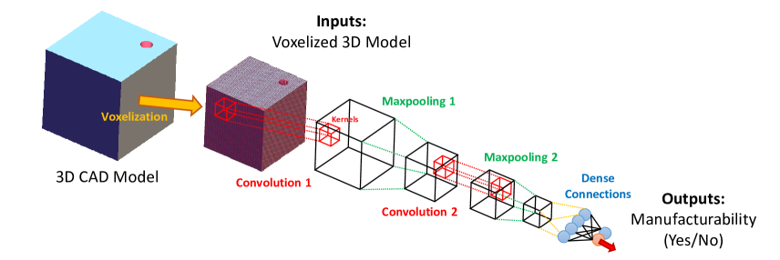
Figure 1: 3D convolutional neural network for the classification of whether or not a design is manufacturable. In this example, a block with a drilled hole with specific diameter and depth is considered.

1 Introduction

Deep learning (DL) algorithms are designed to hierarchically learn multiple levels of abstractions of the data, and have been extensively used in computer vision [1, 2, 3, 4]. More specifically, 3D-Convolutional Neural Networks (3D-CNN) have been used extensively for object recognition, point cloud labeling, video analytics, and human gesture recognition [5, 6, 7, 8]. Object recognition has been one of the most challenging problems in the area of computer vision and pattern recognition. Early DL-based approaches used simple projection of the 3-dimensional object to a 2-dimensional representation such as depth images or multiple views to recognize an object. However, there is a significant loss of geometric information while using a 2D representation of a 3D object. Therefore, it is difficult to learn about the local features of the object using these projection-based techniques. In this paper, we make use of voxelized 3D representation of the object augmented with surface normal information to identify localized features.

Voxelized models have been successfully used in the past for object recognition. Generally, point cloud data is converted to a volume occupancy grid or voxels to represent the model and identify the object. However, voxel-based occupancy grid representation does not inherently have information regarding the surfaces of the object without additional processing. It is also not robust enough to capture information about the location, size, or shape of a feature within an object. Providing additional information about the geometry of the object has been shown to increase the accuracy of object detection by Wang and Siddiqi [9]. In this paper, we propose to use normal information of the surface of the object, in addition to the volume occupancy information, to efficiently learn the local features.

Learning local features in a geometry is different from object recognition. Object recognition is a classification problem, where the object is classified based on a collection of features identified in the object. In this work, we make use of a semi-supervised methodology to learn local features by the DL network, without any specific metric to classify the features. However, we learn localized geometric features of interest within the object based on the cost function of the overall object classification problem. For this purpose, we train a 3D-CNN to learn the key features of the object and also learn the variation in the features that can classify the object for a given cost function.

One of the applications of the aforementioned methodology, which we explore in this paper, is to identify difficult-to-manufacture features in a CAD geometry and ultimately, classify its manufacturability. A successful part or a product needs to meet its specifications, while also being feasible to manufacture. In general, the design engineer ensures that the product is able to function according to the specified requirements and the manufacturing engineer gives feedback to the design engineer about its manufacturability. This process is performed iteratively, often leading to longer product development times and higher costs. There are various handcrafted design for manufacturability (DFM) rules that have been used by the design and manufacturing community to ensure manufacturability of the design based on the manufacturing technology and tools available. However, designing a manufacturable product, with fewer design iterations, depends mainly on the expertise of the design and manufacturing engineer.

Conventional statistical machine learning (ML) models require a lot of hand crafting of the features, which make the DFM problem intractable, since there are many complex manufacturing criteria and rules that need to be satisfied for determining manufacturability [10]. In contrast to this, the hierarchical architecture of DL can be used to learn increasingly complex features by capturing localized geometric features and feature-of-features. Thus, a deep-learning-based design for manufacturing (DLDFM) tool can be used to learn the various DFM rules from different examples of manufacturable and non-manufacturable components without explicit handcrafting. In addition, the learned ML model can be integrated in the CAD system, providing interactive feedback about the manufacturability of the component.

In this paper, we present a 3D Convolutional Neural Network (3D-CNN) based framework that will learn and identify localized geometric features from an expert database in a semi-supervised manner. Further, this is applied to the context of manufacturability with various CAD models classified as manufacturable and non-manufacturable parts. The main contributions of this paper include:

• GPU-accelerated methods for converting CAD models to volume representations (voxelization augmented with surface normals), which can be used to learn localized geometric features.

• A novel voxel-wise 3D gradient-weighted feature localization based on the 3D-CNN framework to identify local features.

• Application of the method to manufacturability analysis of drilled holes.

This paper is arranged as follows. We explain the volume representations that we use for 3D-CNN in Section 2. In Section 3, we discuss the details of the 3D-CNN, including the network architecture and the hyper-parameters. In Section 4, we explain the 3D gradient weighted class activation mapping for identifying the localized geometric features. In Section 5, we discuss the design for manufacturability (DFM) rules used for generation of the datasets for training and testing the 3D-CNN. Finally, in Section 6, we show the results of the deep learning based design for manufacturability (DLDFM) framework in classifying manufacturable and non-manufacturable features and learning capability of the model to identify localized geometric features.

2 Volumetric Representations for Learning Geometric Features

Traditional CAD systems use boundary representations (B-Reps) to define and represent the CAD model  [11]. In B-Reps, the geometry is defined using a set of faces that form the boundary of the solid object. B-Reps are ideally suited for displaying the CAD model by first tessellating the surfaces into triangles and using the GPU to render them. However, learning spatial features using B-Rep can be challenging, since the B-Rep does not contain any volumetric information.

2.1 Voxel based representation of Geometry

In our framework, we convert the B-Rep CAD model to a volumetric occupancy grid of voxels. However, voxelizing a B-Rep CAD model is a compute intensive operation, since the center of each voxel has to be classified as belonging to either inside or outside the model. In addition, thousands of models need to be voxelized during training. Traditional CPU voxelization algorithms are too computationally slow for training the machine learning network in a reasonable time frame. Hence, we have developed methods for accelerated voxelization of CAD models using the graphics processing unit (GPU). These GPU methods are more than 100x faster than the existing state-of-the-art CPU-based methods and can create a voxelized representation of the CAD model with more than 1,000,000,000 voxels. Having a high resolution voxelization will enable us to capture small features in a complex CAD model.

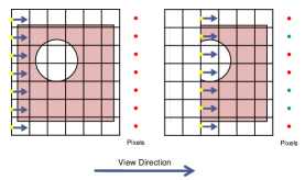
Figure 2: Performing voxelization in 2D using GPU rendering. A clipped CAD model is rendered slice-by-slice and the the number of rendered pixels is counted. The pixels that are rendered an odd number of times in each slice are inside the object (green).

To create the voxelized CAD model, we construct a grid of voxels in the region occupied by the object. We then make use of a rendering-based approach to classify the voxel centers as being inside or outside the object. A 2D example of the method is shown in Figure 2; the method directly extends to 3D. The CAD model is rendered slice-by-slice by clipping it while rendering. Each pixel of this clipped model is then used to classify the voxel corresponding to the slice as being inside or outside the CAD model. This is performed by counting the number of fragments that were rendered in each pixel using the stencil buffer on the GPU. After the clipped model has been rendered, an odd value in the stencil buffer indicates that the voxel on the particular slice is inside the CAD model, and vice versa (Figure 3). The process is then repeated by clipping the model with a plane that is offset by the voxel size. Once all the slices have been classified, we get the complete voxelized representation of the CAD model (Figure 4).

Figure 3: Visualization of voxelized CAD models. The voxels marked in red are outside the model while the voxels marked in green are inside.

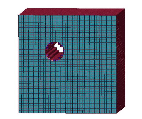
Figure 4: Example voxelized 3D CAD model. The voxels that make up the model are rendered as boxes.

The time taken to perform the classification is the sum of the time taken to tessellate the model once and the total time taken to render each slice. As an example, the total time taken to voxelize the hole block is 0.133 seconds. These timings are obtained by running our voxelization algorithm on a Intel Xeon CPU with 2.4 GHz processor, 64 GB RAM, and an NVIDIA Titan X GPU.

2.2 Augmentation of Surface Normals to volume representation

While a digital voxelized representation may be sufficient for a regular object recognition problem, it may not be enough to capture the detail geometrical information for identifying local fetaures of interest within the object. In particular, information about the boundary is lost in a voxel grid and the local region around a voxel grid need to be analyzed to identify a boundary voxel. To overcome this challenge in voxelized representations, we augment the voxel occupancy grid with the surface normals of the B-Rep geometry. First, we identify the boundary voxels of the B-Rep geometry. We consider each voxel as an axis-aligned bounding-box (AABB) using the center location and size of each voxel. We then find all the triangles of the B-Rep model that intersect with the AABBs. Finally, we average the surface normals of all triangles that intersect with each AABB. The $x,y,\&z$ components of the surface normals are then embedded in the voxelization along with the occupancy grid.

The surface normal information can be augmented with the volume occupancy information in each voxel in two distinct ways:

• The volume occupancy grid and the surface normals are represented independently as four channels (voxel, $X,Y$ and $Z$ directions) for the same object.

• It can be noted that in the previous representation, the normals information exists only on the boundary voxels and is zero all other places in the grid. Alternative representation would be to fuse the volume occupancy grid information with the boundary voxels containing the surface normals (making it 3 channels for the same object).

While one representation is more sparse which might be helpful while training the 3D-CNN, it is also to be noted that more memory is needed while training. In this paper, we explore both the methods of representing the normal information.

3 3D-CNN for Learning Localized Geometric Features

The voxel based representation with the surface normals of the CAD model can be used to train a 3D-CNN that can identify local features. 3D-CNNs have mostly been used for complete 3D object recognition and object generation problems [5, 6, 7, 12, 13, 8] as well as analyzing temporally correlated video frames [14, 15, 16, 17]. However, to the best of the authors’ knowledge, this is the first application of 3D-CNNs on identifying local features with applications in manufacturability analysis.

3.1 Network Architecture and Hyper-Parameters

The input to the 3D-CNN is a voxelized CAD model. The input volumetric data is first padded with zeros before convolution is performed. Zero padding is necessary in this case to ensure that the information about the boundary of the CAD model is not lost while performing the convolution. The convolution layer is applied with RELU activation. The convolutional layer is followed by batch normalization layer and Max. Pooling layer. The same sequence of Convolution, batch normalization and Max. Pooling is again used. A fully connected layer is used before the final output layer with sigmoid activation. The hyper-parameters of the 3D-CNN that needs to be tuned in order to ensure optimal learning. The specific hyper-parameters used in our framework are listed in Section 6.

The model parameters $\theta$, comprised of weights W and biases, b are optimized by error back-propagation with binary cross-entropy as the loss function [18] using the ADADELTA optimizer [19]. Specifically, the loss function $\ell$ to be minimized is:

$$\ell=-y\log{\hat{y}}-(1-y)\log(1-{\hat{y}})$$ (1)

where $y\in\{0,1\}$ is the true class label and $\hat{y}\in\{0,1\}$ is the class prediction.

For training the network, many CAD models were generated based on the method illustrated in section 5.

4 Interpretation of 3D-CNN Output

The trained 3D-CNN network can be used to classify the object of any new geometry and can be treated as a black-box. However, interpretability and explainability of the output provided by the 3D-CNN are very essential. In this paper, we attempt to visualize the input features that lead to a particular output and if possible modify it. A similar approach was used in object recognition in images by using class activation maps to obtain class specific feature maps [20]. The class specific feature maps could be obtained by taking a class discriminative gradient of the prediction with respect to the feature map to get the class activation. In this paper, we present the first application of gradient weighted class activation map (3D-GradCAM) for 3D object recognition.

In order to get the feature localization map using 3D-GradCAM, we need to compute the spatial importance of each feature map $A_{l}$ in the last convolutional layer of the 3D-CNN, for a particular class, $c$ ($c$ can be either non-manufacturability or manufacturability, for the sake of generality) in the classification problem. This spatial importance for each feature map can be interpreted as weights for each feature map; it can be computed as the global average pooling of the gradients back from the specific class of interest as shown in Eqn. 3.

The cumulative spatial importance activations that contribute to the class discriminative localization map, $L_{3DGradCAM}$, is computed using

$$L_{3DGradCAM}=ReLU\left(\sum_{l}{\alpha_{l}\times A^{l}}\right),$$ (2)

where $\alpha_{l}$ are the weights computed using

$$\alpha_{l}=\frac{1}{Z}\times\sum_{i}{\sum_{j}{\sum_{k}{\frac{\partial y^{c}}{\partial A_{ijk}^{l}}}}}.$$ (3)

We can compute the activations obtained for the input part using $L_{3DGradCAM}$ to analyze the source of output. The heat map of $\left(L_{3DGradCAM}\right)$ is resampled using linear interpolation to match the input size, and then overlaid in 3D with the input to be able to spatially identify the source of non-manufacturability. This composite data is finally rendered using a volume renderer.

We make use of a GPU-based ray-marching approach to render this data. The rendering is parallelized on the GPU with each ray corresponding to the screen pixel being cast independently. The intersection of the ray with the bounding-cube of the volumetric data is computed, and then the 3D volumetric data is sampled at periodic intervals. The sum of all the sampled values along the ray is then computed. This value is converted to RGB using a suitable color-bar and rendered on the screen. Table 2 shows different volumetric renderings of the composite 3D-GradCAM data.

5 Manufacturability of Drilled Holes

Design for Manufacturing (DFM) rules for drilling have been traditionally developed based on the parameters of the cylindrical geometry as well as the geometry of the raw material. In this paper, we show an application of our approach to learn localized geometric features to identify non-manufacturability of drilled holes. Deciding the manufacturability of a part is framed as a binary classification problem. We apply the above methodology to learn the parameters that correspond to a hole feature, and then use the learned parameters to classify for manufacturability.

The important geometric parameters of a hole are the diameter, the depth, and the position of the hole. However, there are certain additional geometric parameters that do not contribute to the manufacturability analysis, but might affect the machine learning framework. For example, the face of the stock on which the hole is to be drilled does not affect the manufacturability of the hole, but need to be considered while training because the volumetric representation of the CAD model is not rotationally invariant.

In our DLDFM framework, the following DFM rules are used to classify the drilled hole as manufacturable.

1. Depth-to-diameter ratio: The depth-to-diameter ratio should be less than $5.0$ for the machinability of the hole [21, 22]. It should be noted that this rule is generic and applicable for all materials.

2. Through holes: Since a through hole can be drilled from both directions, the depth-to-diameter ratio for a through hole should be less than $10.0$ to be manufacturable.

3. Holes close to the edges: A manufacturable hole should be surrounded with material of thickness at least equal to the half the diameter of the hole.

4. Thin sections in the depth direction of the hole: A manufacturable hole should should have material greater than half the diameter along the depth direction.

The preceding rules are used to generate the ground truth manufacturability data for the training set, which is then used to learn the manufacturable and non-manufacturable features by the DLDFM Framework. However, it should be noted that for a DLDFM framework, one need not explicitly mention the rule. Rather, for industrial applications, one can train the DLDFM framework using the industry relevant historical data available in the organization, which need not be strictly rule based. The historical data can also be based on experience during previous attempts to manufacture a part. Thus, this DLDFM framework is an attempt to generate a DFM framework based on few basic local features. For more complicated shapes, one can just augment the training set and then re-train the DLDFM framework, which can then be used for analyzing complex parts for manufacturability. This eliminates the hand-crafting of rules, ultimately leading to better manufacturability analysis.

5.1 Training Data

Based on the DFM rules for drilling, different sample solid models are generated using a CAD modeling kernel. We use ACIS [23], a commercial CAD modeling kernel to create the solid models. A cubical block of edge length $5.0$ inches with different sizes of drilled holes are created (Figure 5). The diameter of the hole is varied from $0.1$ in. to $1.0$ in. with an increment of $0.1$ in. Similarly, the depth of the hole is varied from $0.5$ in. to $5.0$ in. with an increment of $0.5$ in. In addition, few geometries are specifically generated with thin sections in the depth direction to make the training data complete. The holes are generated at different positions on the face of the cube by varying the value of $PosX$ and $PosY$ (Figure 5). For sake of simplicity, the holes are located only along the diagonal of the drilling face, i.e. $PosX=PosY$ for all the training samples generated. In addition, the holes are generated in all the six faces of the cube. After the CAD models are generated using the solid modeling kernel, they are classified for manufacturability using the DFM rules for drilled holes.

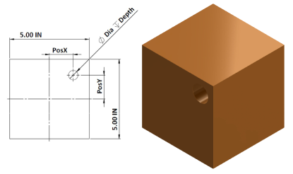
Figure 5: A sample block with a drilled hole with its dimensions highlighted in the projected view.

After the B-Rep models are generated using the CAD modeling kernel, they are converted to volume representations. One of the framework design choices is to choose an appropriate voxel grid for the model. A fine voxelization of the model, while capturing all the features accurately, might be computationally expensive for training the 3D-CNN. Even a voxelization resolution of $64\times 64\times 64$ pushes the limits of the GPU and CPU memory, and hence, the parameters of the 3D-CNN have to be tuned for optimal performance. The complete data is split into training set and validation set.

5.2 Representative and Non-Representative Data

In order to test the performance of the DLDFM network, a new test set of CAD models are generated. The CAD geometry generated in this set is different from the CAD models used in training the DLDFM. Further, we split the test set into two classes, representative and non-representative.

Representative models are broadly defined as those geometries that are related to CAD models in the training set. For example, the DLDFM network was trained using models with a single hole on different faces and at different positions. The geometries in the test set that belong to this subset of the CAD model parameters are classified as representative geometries. However, the models generated in the representative set do not have the same depth or diameter values as those in the models of the training set. For the representative test data, the following parameters are varied to generate the samples.

• Diameter values from $1.1$ to $1.5$ are used for the representative test data. Diameter values from $0.1$ to $1.0$ inches were used for training.

• Position of the holes is varied in the radial directions ($PosX=0$ or $PosY=0$, while the other is varied), as well as in the diagonal direction. The position of the hole vary only in the diagonal direction ($PosX=PoxY$) in the training samples.

Non-representative models are broadly defined as those geometries that are completely different from the training set. The generalization ability of DLDFM can be tested by creating a non-representative test set, containing geometries with the same primary hole parameters (depth, diameter, and position of the hole), but having additional or different external features. The details of the geometries in the non-representative data set is given below.

Multiple holes: The DLDFM has been trained to analyze the manufacturability of a single drilled hole. However, in an a designed component, the features may not be independent; there can be multiple features, each of which may or may not be manufacturable. Moreover, it is possible that each of the features themselves are manufacturable, but due to their proximity or interaction with other features, the part may become non-manufacturable. Hence, we test the ability of the DLDFM framework to analyze the manufacturability of a part with two holes.

L-shaped blocks and cylindrical models: All the models in the training set have an external cubical shape. Hence, to test the capability of DLDFM to capture the manufacturability of a hole irrespective of the external geometry, we use L-shaped Block and cylinders with holes. The rules established in Section 5 also apply to this geometry.

We generated 9531 CAD models in total for the training and validation set. Out of these, 75% of the models were used for training the 3D-CNN and the remaining 25% of the models were used for validation or fine-tuning the hyper-parameters of the 3D-CNN. A detailed description of the training process is provided in Section 3. The trained DLDFM network is then tested using the test set CAD models. The test set contains 675 representative geometries and 1450 non-representative geometries.

=.1in =2.5in Test Data Type Model Description True Positive True Negative False Positive False Negative Accuracy Representative 675 models 408 Manufacturable In-outs Information 391 90 17 176 0.7136 In-outs + Surface Normals 334 201 74 65 0.7938 Coupled In-outs with Surface Normals 405 131 3 135 0.7952 Non-Representative 1450 models 724 Manufacturable In-outs Information 500 422 226 301 0.6363 In-outs + Surface Normals 356 601 370 122 0.6604 Coupled In-outs with Surface Normals 370 582 356 141 0.6570

Table 1: Quantitative performance assessment of the DLDFM on representative and non-representative data sets.

6 Results and Discussion

The different CAD geometries generated as explained in Section 5.1 are classified to be manufacturable or non-manufacturable based on the rules discussed in Section 5. The B-Rep CAD geometries are converted to volumetric representation using voxelization as explained in the Section 2. The grid size of $64\times 64\times 64$ is used for the volumetric representation in order to represent the geometry with sufficient resolution. We initially use the voxelized representation of the CAD geometry to train the DLDFM network. Then, we use the surface normal information (i.e. $x,y,z$ components) in addition to the voxelized representation of the CAD geometry as input. These are considered as four channels of the 3D-CNN input to train another DLDFM network. Since the normal information exists only at the boundary voxels, the three channels (corresponding to the normal components) are very sparse and hence, might be difficult effectively be used by the 3D-CNN. Hence, we fuse the voxelized representation with each of the surface normals (coupled normal information) and provide this as a a three channel input to the 3D-CNN to train the DLDFM network. We set all 3 channels to be 1 inside the object and to be 0 outside the object. The boundary voxels have the value of the 3 channels corresponding to the 3 components of the surface normal.

6.1 Tuning of the Hyper-Parameters

The hyper-parameters for the DLDFM are fine-tuned to have least validation loss. The architecture of the DLDFM network with voxelized information is composed of three convolution layers with filter sizes of 8, 4, and 2 respectively. Likewise, the DLDFM networks using surface normal information along with voxelized representation, comprises of three convolution layers with filter sizes of 6, 3, and 2 respectively. In succession to the first and last Convolution layers, we use MaxPooling layers of subsampling size 2. A batch size of 64 is selected while training all of the three DLDFM networks. The training was performed using Keras [24] with a TensorFlow [25] backend in Python environment. The training of DLDFM networks was performed in a workstation with 128GB CPU RAM and a NVIDIA Titan X GPU with 12GB GPU RAM. The training is run for a lot of epochs and is stopped when the validation loss is not improving for a patience 10 epochs. The training loss vs. validation loss of the DLDFM is shown in Figure 6.

6.2 Test Results

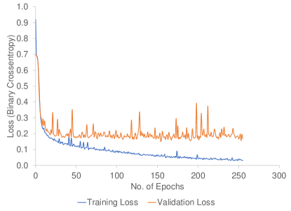
Figure 6: Loss vs. No. of Epochs while training

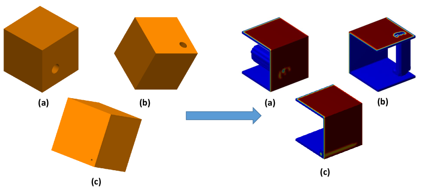
Figure 7: The output of one of the first hidden layer filters in the 3D-CNN architecture. Here, CAD model (a) represents a through hole, CAD model (b) represents a big and deep hole, and CAD model (c) represents a small hole near the corner.

After successful training, the DLDFM network was tested on the representative test-set to benchmark its performance. The voxel based DLDFM network performs well with an accuracy of 71% on 675 models of the representative test set. However, as expected, the performance of the network reduces by a small percentage while testing on the non-representative test set (Table 1). In addition, even though the surface normals augmented DLDFM networks have a poorer training accuracy, their prediction capability on the test-set (both representative and non-representative) is significantly better than the voxel based approach. Specifically, there was a significant improvement in the overall accuracy (a gain of 6%) for predictions in the representative test set as shown in Table 1. Note that the test-set has completely different geometries compared to the training set. Thus, it can be seen that the DLDFM is learning the localized geometric features.

=.2in =2.0in Feature DFM DLDFM Prediction CAD Model 3D-GradCAM Visualization Single hole Manufacturable Manufacturable (Feature: Depth/Diameter ratio of hole $<$ 5) Single hole Non-Manufacturable Non-Manufacturable (Feature: Hole close to the edge) Two holes Same face Non-Manufacturable Non-Manufacturable (Feature: Distance between holes $<$ diameter) L-Block with a hole Non-Manufacturable Non-Manufacturable (Feature: Depth/Diameter ratio of hole $<$ 5) L-Block with a hole Non-Manufacturable Non-Manufacturable (Feature: Hole close to the corner) Two holes Different faces Non-Manufacturable Non-Manufacturable (Feature: One hole is manufacturable One hole is non-manufacturable) Two holes Same face Manufacturable Manufacturable (Feature: Depth/Diameter ratio of both holes $>$ 5) Cylinder with a hole Non-Manufacturable Non-Manufacturable (Feature: Hole close to the edge)

Table 2: Illustrative examples of manufacturability prediction and interpretation using the DLDFM framework.

6.3 Visualization of Feature Maps of 3D-CNN

The ability of the 3D-CNN to learn the local geometric features can be understood by visualizing the feature maps. We provide different sample CAD models to the input of the 3D-CNN and plot the feature maps obtained as output of first layer. The activations are first normalized to one and then the activation tensor for each filter is plotted using the Smooth3 function in MATLAB^®. Figure 7 shows the output obtained from one of the hidden layers of the DLDFM network. It can be seen that the 3D-CNN is able to recognize the primitive information about the geometry; for example, the edges, the faces, the hole, the depth of the hole etc.

6.4 Visualization of 3D-GradCAM

Using the trained DLDFM network, it is possible to obtain the localization of the feature activating the decision of the DLDFM as explained in the Section 4. The 3D-GradCAM renderings for various cases are shown in the Table 2. We have used 3D-GradCAM to visualize the results of various inputs such as manufacturable holes, non-manufacturable-holes, multiple holes in same face, holes in multiple faces of the cube, L shaped block, and cylindrical block. 3D-GradCAM can localize the features that can cause the part to be non-manufacturable. For example, in Table 2, the second example from the top shows a CAD model with a hole, which is non-manufacturable because it is too close to one of side faces. This is a difficult example to classify based only on the information of the hole. The fifth example from the top shows a L-shaped block with a hole at its corner which is non-manufacturable due to its proximity to the edges of the block. The 3D-GradCAM rendering correctly identifies the non-manufacturable hole and as a result the DLDFM network also predicts the part to be non-manufacturable. The feedback is helpful to understand which particular feature among various other features in a CAD geometry that accounts for the non-manufacturability and possibly modify the design appropriately. Finally, the last example in Table 2 shows a non-manufacturable hole inside a cylindrical external geometry. This shows that the 3D-CNN can identify local features irrespective of the external shape of the CAD model. This is again useful to employ the manufacturability analysis.

7 Conclusions and Future work

In this paper, we demonstrate the feasibility of using 3D-CNNs to identify local features of interest using a voxel-based approach. The 3D-CNN was able to learn local geometric features directly from the voxelized model, without any additional shape information. In addition, augmenting the voxel information with surface normals, helped improve the ability of the 3D-CNN to identify local features. As a result, the 3D-CNN was able to identify the local geometric features irrespective of the external object shape, even in the non-representative test data. Hence, a 3D-CNN can be used effectively to identify local features, which in turn can be used to define a metric that may be used for successful object classification.

We apply our novel local fetaure detection tool to build a deep-learning-based DFM (DLDFM) framework which is a novel application of deep learning for cyber-enabled manufacturing. To the best of our knowledge, this is the first application of deep learning to learn the different DFM rules associated with design for manufacturing. In this paper, our DLDFM framework was able to successfully learn the complex DFM rules for drilling, which include not only the depth-to-diameter ratio of the holes but also their position and type (through hole vs. blind). As a consequence, the DLDFM framework out-performs traditional rule-based DFM tools currently available in CAD systems. The framework can be extended to learn manufacturable features for a variety of manufacturing processes such as milling, turning, etc. We envision training multiple networks for specific manufacturing processes, which can be concurrently used to classify the same design with respect to their manufacturability using different processes. Thus, an interactive decision-support system for DFM can be integrated with current CAD systems, which can provide real-time manufacturability analysis while the component is being designed. This would decrease the design time, leading to significant cost-savings.

References

- Sarkar et al. [2015] S. Sarkar, V. Venugopalan, K. Reddy, M. Giering, J. Ryde, and N. Jaitly, “Occlusion edge detection in rgb-d frames using deep convolutional networks,” Proceedings of IEEE High Performance Exterme Computing Conference, Waltham, MA, 2015.
- Lee et al. [2009] H. Lee, R. Grosse, R. Ranganath, and A. Y. Ng, “Convolutional deep belief networks for scalable unsupervised learning of hierarchical representations,” in Proceedings of the 26th annual international conference on machine learning. ACM, 2009, pp. 609–616.
- Lore et al. [2016] K. G. Lore, A. Akintayo, and S. Sarkar, “Llnet: A deep autoencoder approach to natural low-light image enhancement,” Pattern Recognition, 2016.
- Larochelle and Bengio [2008] H. Larochelle and Y. Bengio, “Classification using discriminative restricted boltzmann machines,” in Proceedings of the 25th international conference on Machine learning. ACM, 2008, pp. 536–543.
- Maturana and Scherer [2015a] D. Maturana and S. Scherer, “3D convolutional neural networks for landing zone detection from lidar,” in 2015 IEEE International Conference on Robotics and Automation (ICRA). IEEE, 2015, pp. 3471–3478.
- Maturana and Scherer [2015b] ——, “Voxnet: A 3d convolutional neural network for real-time object recognition,” in Intelligent Robots and Systems (IROS), 2015 IEEE/RSJ International Conference on. IEEE, 2015, pp. 922–928.
- Riegler et al. [2016] G. Riegler, A. O. Ulusoys, and A. Geiger, “Octnet: Learning deep 3d representations at high resolutions,” arXiv preprint arXiv:1611.05009, 2016.
- Huang and You [2016] J. Huang and S. You, “Point cloud labeling using 3d convolutional neural network,” in Proc. of the International Conf. on Pattern Recognition (ICPR), vol. 2, 2016.
- Wang and Siddiqi [2016] C. Wang and K. Siddiqi, “Differential geometry boosts convolutional neural networks for object detection,” in Proceedings of the IEEE Conference on Computer Vision and Pattern Recognition Workshops, 2016, pp. 51–58.
- Shukor and Axinte [2009] S. A. Shukor and D. Axinte, “Manufacturability analysis system: issues and future trends,” International Journal of Production Research, vol. 47, no. 5, pp. 1369–1390, 2009.
- Krishnamurthy et al. [2009] A. Krishnamurthy, R. Khardekar, and S. McMains, “Optimized GPU evaluation of arbitrary degree nurbs curves and surfaces,” Computer-Aided Design, vol. 41, no. 12, pp. 971–980, 2009.
- Riegler et al. [2017] G. Riegler, A. O. Ulusoy, H. Bischof, and A. Geiger, “Octnetfusion: Learning depth fusion from data,” arXiv preprint arXiv:1704.01047, 2017.
- Tatarchenko et al. [2017] M. Tatarchenko, A. Dosovitskiy, and T. Brox, “Octree generating networks: Efficient convolutional architectures for high-resolution 3d outputs,” arXiv preprint arXiv:1703.09438, 2017.
- Ji et al. [2013] S. Ji, W. Xu, M. Yang, and K. Yu, “3d convolutional neural networks for human action recognition,” IEEE transactions on pattern analysis and machine intelligence, vol. 35, no. 1, pp. 221–231, 2013.
- Tran et al. [2015] D. Tran, L. Bourdev, R. Fergus, L. Torresani, and M. Paluri, “Learning spatiotemporal features with 3d convolutional networks,” in 2015 IEEE International Conference on Computer Vision (ICCV). IEEE, 2015, pp. 4489–4497.
- Payan and Montana [2015] A. Payan and G. Montana, “Predicting alzheimer’s disease: a neuroimaging study with 3d convolutional neural networks,” arXiv preprint arXiv:1502.02506, 2015.
- Lee et al. [2015] K. Lee, A. Zlateski, A. Vishwanathan, and H. S. Seung, “Recursive training of 2d-3d convolutional networks for neuronal boundary detection,” arXiv preprint arXiv:1508.04843, 2015.
- Hinton and Salakhutdinov [2006] G. E. Hinton and R. R. Salakhutdinov, “Reducing the dimensionality of data with neural networks,” Science, vol. 313, no. 5786, pp. 504–507, 2006.
- Zeiler [2012] M. D. Zeiler, “Adadelta: an adaptive learning rate method,” arXiv preprint arXiv:1212.5701, 2012.
- Selvaraju et al. [2016] R. R. Selvaraju, A. Das, R. Vedantam, M. Cogswell, D. Parikh, and D. Batra, “Grad-cam: Why did you say that? visual explanations from deep networks via gradient-based localization,” arXiv preprint arXiv:1610.02391, 2016.
- Boothroyd et al. [2002] G. Boothroyd, P. Dewhurst, and W. Knight, Product Design for Manufacture and Assembly. M. Dekker, 2002.
- Bralla [1999] J. G. Bralla, Design for manufacturability handbook. McGraw-Hill,, 1999.
- Spatial Corporation [2009] Spatial Corporation, ACIS Geometric Modeler: User Guide, 2009, version 20.0.
- Chollet [2015] F. Chollet, “Keras,” https://github.com/fchollet/keras, 2015.
- Abadi et al. [2015] M. Abadi, A. Agarwal, P. Barham, E. Brevdo, Z. Chen, C. Citro, G. S. Corrado, A. Davis, J. Dean, M. Devin, S. Ghemawat, I. Goodfellow, A. Harp, G. Irving, M. Isard, Y. Jia, R. Jozefowicz, L. Kaiser, M. Kudlur, J. Levenberg, D. Mané, R. Monga, S. Moore, D. Murray, C. Olah, M. Schuster, J. Shlens, B. Steiner, I. Sutskever, K. Talwar, P. Tucker, V. Vanhoucke, V. Vasudevan, F. Viégas, O. Vinyals, P. Warden, M. Wattenberg, M. Wicke, Y. Yu, and X. Zheng, “TensorFlow: Large-scale machine learning on heterogeneous systems,” 2015, software available from tensorflow.org. [Online]. Available: http://tensorflow.org/