Scaling and universality in the phase diagram of the 2D Blume-Capel model

Abstract

We review the pertinent features of the phase diagram of the zero-field Blume-Capel model, focusing on the aspects of transition order, finite-size scaling and universality. In particular, we employ a range of Monte Carlo simulation methods to study the 2D spin-1 Blume-Capel model on the square lattice to investigate the behavior in the vicinity of the first-order and second-order regimes of the ferromagnet-paramagnet phase boundary, respectively. To achieve high-precision results, we utilize a combination of (i) a parallel version of the multicanonical algorithm and (ii) a hybrid updating scheme combining Metropolis and generalized Wolff cluster moves. These techniques are combined to study for the first time the correlation length of the model, using its scaling in the regime of second-order transitions to illustrate universality through the observed identity of the limiting value of $\xi/L$ with the exactly known result for the Ising universality class.

1 Introduction

The Blume-Capel (BC) model is defined by a spin-1 Ising Hamiltonian with a single-ion uniaxial crystal field anisotropy blume ; capel . The fact that it has been very widely studied in statistical and condensed-matter physics is explained not only by its relative simplicity and the fundamental theoretical interest arising from the richness of its phase diagram, but also by a number of different physical realizations of variants of the model, ranging from multi-component fluids to ternary alloys and ³He–⁴He mixtures lawrie . Quite recently, the BC model was invoked by Selke and Oitmaa in order to understand properties of ferrimagnets selke-10 .

The zero-field model is described by the Hamiltonian

$$\mathcal{H}=-J\sum_{\langle ij\rangle}\sigma_{i}\sigma_{j}+\Delta\sum_{i}\sigma_{i}^{2}=E_{J}+\Delta E_{\Delta},$$ (1)

where the spin variables $\sigma_{i}$ take on the values $-1,0$, or $+1$, $\langle ij\rangle$ indicates summation over nearest neighbors only, and $J>0$ is the ferromagnetic exchange interaction. The parameter $\Delta$ is known as the crystal-field coupling and it controls the density of vacancies ($\sigma_{i}=0$). For $\Delta\rightarrow-\infty$, vacancies are suppressed and the model becomes equivalent to the Ising model. Note the decomposition on the right-hand side of Eq. (1) into the bond-related and crystal-field-related energy contributions $E_{J}$ and $E_{\Delta}$, respectively, that will turn out to be useful in the context of the multicanonical simulations discussed below.

Since its original formulation, the model (1) has been studied in mean-field theory as well as in perturbative expansions and numerical simulations for a range of lattices, mostly in two and three dimensions, see, e.g., Refs. fytas_BC ; zierenberg2015 . Most work has been devoted to the two-dimensional model, employing a wide range of methods including real space renormalization berker1976rg , Monte Carlo (MC) simulations and MC renormalization-group calculations landau1972 ; kaufman1981 ; selke1983 ; selke1984 ; landau1986 ; xavier1998 ; deng2005 ; silva2006 ; hurt2007 ; malakis ; kwak2015 , $\epsilon$-expansions stephen1973 ; chang1974 ; tuthill1975 ; wegner1975 , high- and low-temperature series expansions fox1973 ; camp1975 ; burkhardt1976 and a phenomenological finite-size scaling (FSS) analysis beale1986 . In the present work, we focus on the nearest-neighbor square-lattice case and use a combination of multicanonical and cluster-update Monte Carlo simulations to examine the first-order and second-order regimes of the ferromagnet-paramagnet phase boundary. One focus of this work is a study of the correlation length of the model, a quantity which to our knowledge has not been studied before in this context. We locate transition points in the phase diagram of the model for a wide temperature range, thus allowing for comparisons with previous work. In the second-order regime, we show that the correlation-length ratio $\xi/L$ for finite lattices tends to the exactly known value of the 2D Ising universality class, thus nicely illustrating universality.

The rest of the paper is organized as follows. In Sec. 2 we briefly review the qualitative and some simple quantitative features of the phase diagram in two dimensions. Section 3 provides a thorough description of the simulation methods, the relevant observables and FSS analyses. In Sec. 4 we use scaling techniques to elucidate the expected behaviors in the first-order regime as well as the universality of the exponents and the ratio $\xi/L$ for the parameter range with continuous transitions. In particular, here we demonstrate Ising universality by the study of the size evolution of the universal ratio $\xi/L$. Finally, Sec. 5 contains our conclusions.

2 Phase diagram of the Blume-Capel model

The general shape of the phase diagram of the model is that shown in Fig. 1. While this presentation, comprising selected previous results beale1986 ; silva2006 ; malakis ; kwak2015 together with estimates from the present work, is for the square-lattice model, the general features of the phase diagram are the same for higher dimensions also blume ; capel . The phase boundary separates the ferromagnetic (F) from the paramagnetic (P) phase. The ferromagnetic phase is characterized by an ordered alignment of $\pm 1$ spins. The paramagnetic phase, on the other hand, can be either a completely disordered arrangement at high temperature or a $\pm 1$-spin gas in a $0$-spin dominated environment for low temperatures and high crystal fields. At high temperatures and low crystal fields, the F–P transition is a continuous phase transition in the Ising universality class, whereas at low temperatures and high crystal fields the transition is of first order blume ; capel . The model is thus a classic and paradigmatic example of a system with a tricritical point $(\Delta_{\rm t},T_{\rm t})$ lawrie , where the two segments of the phase boundary meet. At zero temperature, it is clear that ferromagnetic order must prevail if its energy $zJ/2$ per spin (where $z$ is the coordination number) exceeds that of the penalty $\Delta$ for having all spins in the $\pm 1$ state. Hence the point $(\Delta_{0}=zJ/2,T=0)$ is on the phase boundary capel . For zero crystal-field $\Delta$, the transition temperature $T_{0}$ is not exactly known, but well studied for a number of lattice geometries.

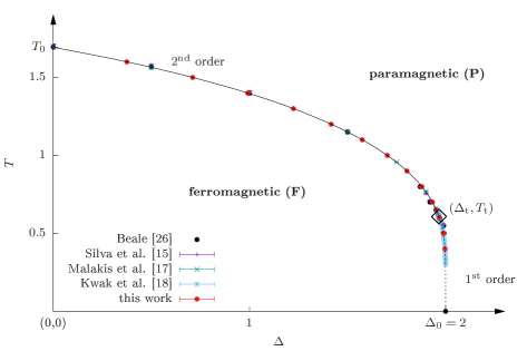
Figure 1: Phase diagram of the square-lattice, zero-field BC model in the $\Delta$–$T$ plane. The phase boundary separates the ferromagnetic (F) phase from the paramagnetic (P) phase. The solid line indicates continuous phase transitions and the dotted line marks first-order phase transitions. The two lines merge at the tricritical point $(\Delta_{\rm t},T_{\rm t})$, as highlighted by the black diamond. The data shown are selected estimates from previous studies as well as the present work. The numerical values of all individual estimates are summarized in Table 1 below.

In the following, we consider the square lattice and fix units by choosing $J=1$ and $k_{\rm B}=1$. The estimates shown in Fig. 1 for this case are based on phenomenological FSS using the transfer matrix for systems up to size $L=10$ beale1986 , standard Wang-Landau simulations up to $L=100$ malakis , two-parameter Wang-Landau simulations up to $L=16$ silva2006 and $L=48$ kwak2015 , as well as the results of the present work, using parallel multicanonical simulations at fixed temperature up to $L=128$ ($T>T_{\rm t}$) and $L=96$ ($T<T_{\rm t}$). A subset of these results is summarized in Table 1 for comparison. Note that in the multicanonical simulations employed in the present work we fix the temperature $T$ while varying the crystal field $\Delta$ zierenberg2015 , whereas crossings of the phase boundary at constant $\Delta$ were studied in most other works. In general, we find excellent agreement between the recent large-scale simulations. Some deviations of the older results, especially in the first-order regime, are probably due to the small system sizes studied. We have additional information for $T=0$ where $\Delta_{0}=zJ/2=2$ and for $\Delta=0$, where results from high- and low-temperature series expansions for the spin-1 Ising model provide $T_{0}=1.690(6)$ fox1973 ; camp1975 ; burkhardt1976 , while phenomenological finite-size scaling yields $T_{0}\simeq 1.695$ beale1986 , one-parametric Wang-Landau simulations give $T_{0}=1.693(3)$ malakis , and two-parametric Wang-Landau simulations arrive at $T_{0}=1.714(2)$ silva2006 . Overall, the first three results are in very good agreement. The deviations observed for the result of the two-parametric Wang-Landau approach silva2006 can probably be attributed to the relatively small system sizes studied there. Determinations of the location of the tricritical point are technically demanding as the two parameters $T$ and $\Delta$ need to be tuned simultaneously. Early attempts include MC simulations, $[\Delta_{\rm t}=1.94,T_{\rm t}=0.67]$ landau1972 ; selke1983 ; selke1984 , and real-space renormalization-group calculations, $[\Delta_{\rm t}=1.97,T_{\rm t}=0.580]$ berker1976rg ; burkhardt1976rg ; burkhardt1977rg ; kaufmann1981rg ; yeomans1981rg . More precise and mostly mutually consistent estimates were obtained by phenomenological finite-size scaling, $[\Delta_{\rm t}=1.9655(50),T_{\rm t}=0.610(5)]$ beale1986 , MC renormalization-group calculations, $[\Delta_{\rm t}=1.966(15),T_{\rm t}=0.609(3)]$ landau1986 , MC simulations with field mixing, $[\Delta_{\rm t}=1.9665(3),T_{\rm t}=0.608(1)]$ wilding1996 and $[\Delta_{\rm t}=1.9665(3),T_{\rm t}=0.608(1)]$ plascak2013 , transfer matrix and conformal invariance, $[\Delta_{\rm t}=1.965(5),T_{\rm t}=0.609(4)]$ xavier1998 , and two-parametric Wang-Landau simulations, $[\Delta_{\rm t}=1.966(2),T_{\rm t}=0.609(3)]$ silva2006 and $[\Delta_{\rm t}=1.9660(1),T_{\rm t}=0.6080(1)]$ kwak2015 .

Below the tricritical temperature, $T<T_{\rm t}$, or for crystal fields $\Delta>\Delta_{\rm t}$, the model exhibits a first-order phase transition. This is signaled by a double peak in the probability distribution of a field-conjugate variable. This is commonly associated with a free-energy barrier and the corresponding interface tension. Finite-size scaling for first-order transitions predicts a shift of pseudo-critical points according to binder

$$\Delta_{L}^{\ast}=\Delta^{\ast}+aL^{-D},$$ (2)

where $\Delta^{\ast}$ denotes the transition field in the thermodynamic limit and $D$ is the dimension of the lattice. Note that a completely analogous expression holds for the shifts $T_{L}^{\ast}$ in temperature when crossing the phase boundary at fixed $\Delta$. Higher-order corrections are of the form $V^{-n}=L^{-nD}$ with $n\geq 2$, where $V$ is the system volume, but exponential corrections can also be relevant for smaller system sizes janke1st . The phase coexistence at the transition point is connected with the occurrence of a latent heat or latent magnetization that lead to a divergence of the specific heat $C$ and the magnetic susceptibility $\chi$, evaluated at the pseudo-critical point, where both show a pronounced peak: $C_{L}^{\ast}=C(\Delta_{L}^{\ast})\sim L^{D}$ and $\chi_{L}^{\ast}=\chi(\Delta_{L}^{\ast})\sim L^{D}$.

Above the tricritical temperature $T>T_{\rm t}$, or for crystal fields $\Delta<\Delta_{\rm t}$, the model exhibits a second-order phase transition. This segment of the phase boundary is expected to be in the Ising universality class beale1986 . The shifts of pseudo-critical points hence follow LandBind00

$$\Delta_{L}^{\ast}=\Delta_{\rm c}+aL^{-1/\nu},$$ (3)

where $\nu$ is the critical exponent of the correlation length. An analogous expression can again be written down for the case of crossing the phase boundary at constant $\Delta$. The relevant exponents for the Ising universality class are the well-known Onsager ones, i.e., $\alpha=0$, $\beta=1/8$, $\gamma=7/4$, and $\nu=1$. Corrections to the form (3) can include analytic and confluent terms, for a discussion see, e.g., Ref. cardy_book . Since $\alpha=0$ we expect a merely logarithmic divergence of the specific-heat peaks, $C_{L}^{\ast}\sim\ln L$. The peaks of the magnetic susceptibility should scale as $\chi_{L}^{\ast}\sim L^{\gamma/\nu}$. We recall that critical exponents are not the only universal quantities cardy_book , as these are accompanied by critical amplitude ratios such as the ratio $U_{\xi}=f^{+}/f^{-}$ of the amplitude of the correlation length scaling $\xi\sim f^{\pm}t^{-\nu}$ above and below the critical point pelissetto2002 . Less universal are dimensionless quantities in finite-size scaling such as the ratio of the correlation length and the system size, $\xi/L$, which for Ising spins on $L\times L$ patches of the square lattice with periodic boundary conditions for $L\to\infty$ approaches the value salas2000

$$(\xi/L)_{\infty}=0.905\,048\,829\,2(4).$$ (4)

We will study this ratio below for the present system in the second-order regime. Another weakly universal quantity is the fourth-order magnetization cumulant (Binder parameter) $V_{4}$ at criticality selke2005 ; pelissetto2002 .

3 Simulation methods and observables

For the present study we used a combination of two advanced simulational setups. The bulk of our simulations are performed using a generalized parallel implementation of the multicanonical approach. Comparison tests and illustrations of universality are conducted via a hybrid updating scheme combining Metropolis and generalized Wolff cluster updates. The multicanonical approach is particularly well suited for the first-order transition regime of the phase diagram and enables us to sample a broad parameter range (temperature or crystal field). It also yields decent estimates for the transition fields in the second-order regime and the corresponding quantities of interest. For such continuous transitions, the hybrid approach may then be applied subsequently in the vicinity of the already located pseudo-critical points in order to obtain results of higher accuracy. In all our simulations we keep a constant temperature and cross the phase boundary along the crystal-field axis, in analogy to our recent study in three dimensions zierenberg2015 .

3.1 Parallel multicanonical approach

The original multicanonical (muca) method berg1991 ; janke1992 introduces a correction function to the canonical Boltzmann weight $\exp(-\beta E)$, where $\beta=1/(k_{\rm B}T)$ and $E$ is the energy, that is designed to produce a flat histogram after iterative modification. This can be interpreted as a generalized ensemble over the phase space $\{\phi\}$ of configurations ($\{\phi\}=\{\sigma_{i}\}$ for the BC model) with weight function $W[{\cal H}(\{\phi\})]$, where ${\cal H}$ is the Hamiltonian and $E={\cal H}(\{\phi\})$. The corresponding generalized partition function is

$$Z_{\rm muca}=\int_{\{\phi\}}W[{\cal H}(\{\phi\})]\,\mathrm{d}\{\phi\}=\int\Omega(E)W(E)\,\mathrm{d}E.$$ (5)

As the second form shows, a flat energy distribution $P_{\mathrm{muca}}(E)=\Omega(E)W(E)/Z_{\mathrm{muca}}={\rm const}.$ is achieved if $W(E)\propto\Omega^{-1}(E)$, i.e., if the weight is inversely proportional to the density of states $\Omega(E)$. For the weight function $W^{(n)}(E)$ in iteration $n$, the resulting normalized energy histogram satisfies $\langle H^{(n)}(E)\rangle=P^{(n)}(E)=\Omega(E)W^{(n)}(E)/Z^{(n)}$. This suggests to choose as weight function $W^{(n+1)}(E)=W^{(n)}(E)/H^{(n)}(E)$ for the next iteration, thus iteratively approaching $W(E)\propto\Omega^{-1}(E)$. In each of the ensembles defined by $W^{(n)}$, we can still estimate canonical expectation values of observables $O=O(\{\phi\})$ without systematic deviations as

$$\langle O\rangle_{\beta}=\frac{\langle O(\{\phi\})e^{-\beta{\cal H}(\{\phi\})}W^{-1}[{\cal H}(\{\phi\})]\rangle_{\rm muca}}{\langle e^{-\beta{\cal H}(\{\phi\})}W^{-1}[{\cal H}(\{\phi\})]\rangle_{\rm muca}}.$$ (6)

For the present problem we apply the generalized ensemble approach to the crystal-field component $E_{\Delta}$ of the energy only, thus allowing us to continuously reweight to arbitrary values of $\Delta$ zierenberg2015 . To this end, we fix the temperature and apply a generalized configurational weight according to

$$e^{-\beta(E_{J}+\Delta E_{\Delta})}\rightarrow e^{-\beta E_{J}}~{}W\left(E_{\Delta}\right).$$ (7)

The procedure of weight iteration is applied in exactly the same way as before. Data from a final production run with fixed $W(E_{\Delta})$ may be reweighted to the canonical ensemble via a generalization of Eq. (6),

$$\langle O\rangle_{\beta,\Delta}=\frac{\langle Oe^{-\beta\Delta E_{\Delta}}W^{-1}(E_{\Delta})\rangle_{\rm muca}}{\langle e^{-\beta\Delta E_{\Delta}}W^{-1}(E_{\Delta})\rangle_{\rm muca}}.$$ (8)

As was demonstrated in Ref. zierenberg2013 , the multicanonical weight iteration and production run can be efficiently implemented in a parallel fashion. To this end, parallel Markov chains sample independently with the same fixed weight function $W^{(n)}(E_{\Delta})$. After each iteration, the histograms are summed up and form independent contributions to the probability distribution $H^{(n)}(E_{\Delta})=\sum_{i}H^{(n)}_{i}(E_{\Delta})$. In the present case, we ran our simulations with $64$ parallel threads and demanded a flat histogram in the range $E_{\Delta}\in[0,V]$ with a total of $200$ transits, where $V=L^{2}$ is the total number of lattice sites. A transit was here defined as a single Markov chain traveling from one energy boundary to another.

Using this parallelized multicanonical scheme we performed simulations at various fixed temperatures, cf. the data collected below in Table 1 in the summary section. For each $T$, we simulated system sizes up to $L_{\rm max}=128$ in the second-order regime of the phase diagram ($T>T_{\rm t}$) and up to $L_{\rm max}\leq 96$ (depending on the temperature) in the first-order regime ($T<T_{\rm t}$). At one particular temperature, namely $T=1.398$, we were able to compare with several previous, in part contradictory, studies beale1986 ; silva2006 ; malakis .

3.2 Hybrid approach

For the second-order regime of the phase boundary, our simulations need to cope with the critical slowing down effect that is not explicitly removed by the multicanonical approach. Here, we make use of a suitably constructed cluster-update algorithm to achieve precise estimates close to criticality. While the Fortuin-Kasteleyn representation of the Ising and Potts models Fortuin1972 allows for a drastic reduction or, in some cases, removal of critical slowing down using cluster updates swendsen:87a , the situation is more involved for the BC model, where no complete transformation to a dual bond language is available. As suggested previously in Refs. Blote95 ; hasen2010 ; malakis12 , we therefore rely on a partial transformation, applying a cluster update only to the spins in the $\pm 1$ states, ignoring the diluted sites with $\sigma_{i}=0$. This approach alone is clearly not ergodic as the number and location of $\sigma_{i}=0$ sites is invariant, and we hence supplement it by a local Metropolis update. For the cluster update of the $\pm 1$ spins we use the single-cluster algorithm due to Wolff Wolff1989 . In the present hybrid approach an elementary MC step (MCS) is the following heuristically determined mixture: after each Wolff step we attempt $3\times L$ Metropolis spin flips and the elementary step consists of $L$ such combinations. In other words, a MCS has $3$ Metropolis sweeps and $L$ Wolff steps.

The convergence of the hybrid approach may be easily checked for every lattice size used in the simulations. For instance, to observe convergence for $L=24$ we used $3$ different runs consisting of $12800\times V$, $25600\times V$, and $51200\times V$ (about $30\times 10^{6}$) MCS, whereas for $L=48$ we compared another set of $3$ different runs consisting of $2560\times V$, $5120\times V$, and $10240\times V$ (about $23\times 10^{6}$) MCS. In all our simulations a first large number of MCS was disregarded until the system was well equilibrated. Our runs using this technique covered a range of different temperatures in the second-order regime and, in particular, the selected temperature $T=1.398$ mentioned above, using system sizes up to $L_{\rm max}=128$. For each $L$, we used up to $100$ independent runs performed in parallel to increase our statistical accuracy.

(a)                                                   (b)

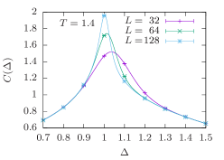
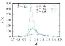
Figure 2: Specific heat (a) and susceptibility (b) curves as a function of the crystal field $\Delta$ obtained from parallel multicanonical simulations at $T=1.4$ The lines show simulation results as continuous functions of $\Delta$ from reweighting, the individual points indicate the size of statistical errors.

3.3 Observables

For the purpose of the present study we focused on the specific heat, the magnetic susceptibility and the correlation length. As in our simulations we cross the transition line at fixed temperature, it is reasonable to study the crystal-field derivative $\partial\langle E\rangle/\partial\Delta$ instead of the temperature gradient $\partial\langle E\rangle/\partial T$. As was pointed out in Ref. zierenberg2015 , the singular behavior is also captured in the simpler quantity

$$C\equiv\frac{\partial\langle E_{J}\rangle}{\partial\Delta}\frac{1}{V}=-\beta\left(\langle E_{J}E_{\Delta}\rangle-\langle E_{J}\rangle\langle E_{\Delta}\rangle\right)/V.$$ (9)

The magnetic susceptibility is defined as the field derivative of the absolute magnetization, and this yields

$$\chi=\beta\left(\langle M^{2}\rangle-\langle|M|\rangle^{2}\right)/V,$$ (10)

where $M=\sum_{i}\sigma_{i}$. As we will discuss below, however, the use of the modulus $|M|$ to break the symmetry on a finite lattice leads to some subtleties for the BC model, especially in the first-order regime. Exemplary plots of $C$ and $\chi$ as a function of the crystal field $\Delta$ obtained from the multicanonical simulations are shown in Fig. 2. It is obvious from these plots that both $C(\Delta)$ and $\chi(\Delta)$ show a size-dependent maximum, together with a shift behavior of peak locations.

Let us define $\Delta^{\ast}_{L,C}$ and $\Delta^{\ast}_{L,\chi}$ as the crystal-field values which maximize $C(\Delta)$ and $\chi(\Delta)$, respectively. These are pseudo-critical points that should scale according to Eqs. (2) and (3), respectively. They are numerically determined by a bisection algorithm that iteratively performs histogram reweighting in the vicinity of the peak, detecting the point of locally vanishing slope. Error bars are obtained by repeating this procedure for 32 jackknife blocks efron1982 . Similarly, we denote by $C^{\ast}_{L}=C(\Delta^{\ast}_{L,C})$ and $\chi^{\ast}_{L}=\chi(\Delta^{\ast}_{L,\chi})$ the values of the specific heat and the magnetic susceptibility at their pseudo-critical points, respectively. These may be directly evaluated as canonical expectation values according to Eq. (8).

We finally also studied the second-moment correlation length $\xi$ cooper1989 ; ballesteros2001 . This involves the Fourier transform of the spin field $\hat{\sigma}(\mathbf{k})=\sum_{\bf x}\sigma_{\bf x}e^{i{\bf kx}}$. If we set $F=\left\langle|\hat{\sigma}(2\pi/L,0)|^{2}+|\hat{\sigma}(0,2\pi/L)|^{2}\right\rangle/2$, the correlation length can be obtained via ballesteros2001

$$\xi\equiv\frac{1}{2\sin(\pi/L)}\sqrt{\frac{\langle M^{2}\rangle}{F}-1}.$$ (11)

From $\xi$ we may compute the ratio $\xi/L$, which tends to a weakly universal constant for $L\to\infty$ as discussed above in Sec. 2.

4 Numerical results

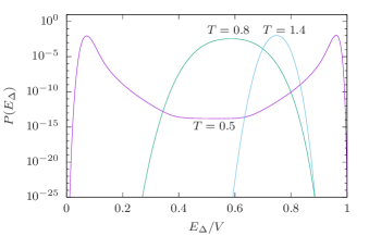
Figure 3: Canonical probability distribution $P(E_{\Delta})$ at the transition field $\Delta_{L,C}^{\ast}$ for various temperatures for $L=48$. Note the logarithmic scale on the vertical axis.

In this section we present our main finite-size scaling analysis, covering both first- and second-order transition regimes of the phase diagram of the square-lattice model. We begin by presenting the canonical probability distribution $P(E_{\Delta})$ at the pseudo-critical crystal fields $\Delta^{\ast}_{L,C}$ for different temperatures. Figure 3 shows $P(E_{\Delta})$ for the temperature $T=0.5$, which is in the first-order regime, and for $T=0.8$ and $1.4$, which are in the second-order regime of the transition line, for a system size $L=48$. Well inside the first-order transition regime the system shows a strong suppression of transition states, connected to a barrier between two coexisting phases. This is characteristic of a discontinuous transition. Here, the barrier separates a spin-$0$ dominated (small $E_{\Delta}$, $\Delta>\Delta^{\ast}$) and a spin-$\pm 1$ dominated (large $E_{\Delta}$, $\Delta<\Delta^{\ast}$) phase. In this regime, the model qualitatively describes the superfluid transition in ³He-⁴He mixtures. As the temperature increases and exceeds the tricritical point $T_{\rm t}\approx 0.608$, the barrier disappears and the probability distribution shows a unimodal shape, characteristic of a continuous transition. In this regime the model qualitatively describes the lambda line of ³He-⁴He mixtures.

First-order regime:

Here we focus on one particular temperature, namely $T=0.5$, to verify the expected scaling discussed in Sec. 2. Figure 4(a) shows a finite-size scaling analysis of the pseudo-critical fields for which we expect shifts of the form

$$\Delta^{\ast}_{L,O}=\Delta^{\ast}+a_{O}L^{-x}.$$ (12)

We performed simultaneous fits to $\Delta^{\ast}_{L,C}$ and $\Delta^{\ast}_{L,\chi}$ with a common value of $x$. Including the full range of data $L=8-96$ we obtain $\Delta^{\ast}=1.987\,893(6)$ and $x=2.03(4)$ with $Q\approx 0.98$. This is consistent with the most recent and very precise estimate $\Delta^{\ast}=1.987\,89(1)$ by Kwak et al. kwak2015 , and the theoretical prediction $x=D=2$. We note that for all fits performed here, we chose a minimum system size to include in the fit such that a goodness-of-fit parameter $Q>0.1$ was achieved. For the specific heat at the maxima, we expect the leading behavior $C^{\ast}_{L}\sim L^{D}$. Scaling corrections at first-order transitions are in inverse integer powers of the volume janke1st , $L^{-nD}$, $n=1$, $2$, $\ldots$, so we attempted the fit form

$$C^{\ast}_{L}=b_{C}L^{x}\left(1+b^{\prime}_{C}L^{-2}\right)$$ (13)

and we indeed find an excellent fit for the full range of system sizes, yielding $x=1.9999(2)$ and $Q=0.78$ — note that due to the value of $x$, the $1/L^{2}$ correction simply corresponds to an additive constant. The amplitudes are $b_{C}=0.8065(6)$ and $b^{\prime}_{C}=0.84(5)$. This fit and the corresponding data are shown in Fig. 4(b).

(a)                                                   (b)

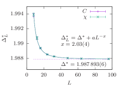
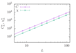
Figure 4: Finite-size scaling analysis in the first-order transition regime ($T=0.5$) based on the specific heat and magnetic susceptibility. (a) Simultaneous fit of the functional form (12) to the pseudo-critical fields of the specific heat and susceptibility. (b) Scaling of the values $C_{L}^{\ast}$ and $\chi_{L}^{\ast}$ at these maxima together with fits of the form (13) and (14) to the data.

For the magnetic susceptibility, on the other hand, the correction proportional to $L^{-2}$ is not sufficient to describe the data down to small $L$, and neither are higher orders $L^{-4}$, $L^{-6}$ etc. We also experimentally included an exponential correction which is expected to occur in the first-order scenario and occasionally can be relevant for small $L$ janke1st , but this also did not lead to particularly good fits. Using an additional $1/L$ correction, on the other hand, i.e., a fit form

$$\chi^{\ast}_{L}=b_{\chi}L^{x}\left(1+b^{\prime}_{\chi}L^{-1}+b^{\prime\prime}_{\chi}L^{-2}\right)$$ (14)

yields excellent results with $Q=0.98$ and $x=2.001(1)$ for the full range $L=8$–$96$ of system sizes, the corresponding fit and data are also shown in Fig. 4(b). Here, $b_{\chi}=0.458(2)$, $b^{\prime}_{\chi}=-0.94(5)$ and $b^{\prime\prime}_{\chi}=2.5(3)$. A $1/L$ correction term is not expected at a first-order transition janke1st , but its presence is rather clear from our data. Some further consideration reveals that it is, in fact, an artifact resulting from the use of the modulus $|M|$ in defining $\chi$ in Eq. (10). To see this, consider the shape of the magnetization distribution function at the transition point $\Delta^{\ast}_{L,\chi}$ shown for different system sizes in Fig. 5(a). The middle peak corresponds to the disordered phase dominated by $0$-spins, while the peaks on the left and right represent the ordered $\pm 1$ phases. While in $P(M)$, the middle peak is symmetric around zero and hence $\langle M\rangle_{d}=0$ in the disordered phase, the modulus $|M|$ will lead to an average $\langle|M|\rangle_{d}=O(L)$ of the order of the peak width. Since $\chi$ measures the square width of the distribution of $|M|$, this will have a $1/L$ correction stemming from this $O(L)$ contribution to $|M|$.

This problem can be avoided by employing a different method of breaking the symmetry on a finite lattice. One possible definition could be

$$\widetilde{M}=\left\{\begin{array}[]{l@{\hspace{0.75em}}l}M\hfil\hskip 7.5pt&\mbox{for}\;\;|M|/V<0.5\\ |M|\hfil\hskip 7.5pt&\mbox{for}\;\;|M|/V\geq 0.5\end{array}\right.,$$ (15)

which only folds the $-1$-peak onto the $+1$-peak, but leaves the $0$-peak untouched. As is seen from the data and fits shown in Fig. 5(b) in contrast to $\chi$ the scaling of the corresponding susceptibility $\widetilde{\chi}=\beta(\langle\widetilde{M}^{2}\rangle-\langle\widetilde{M}\rangle^{2})/V$ does not show a $1/L$ correction, but only the volume correction $\propto 1/L^{2}$ expected for a first-order transition.

Overall, it is apparent that our simulations nicely reproduce the behavior expected for a first-order transition, whereas a conventional canonical-ensemble simulation scheme would be hampered by metastability and hyper-critical slowing down.

(a)                                                   (b)

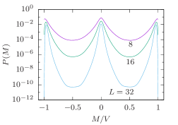
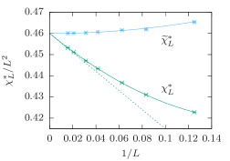
Figure 5: (a) Canonical probability distribution $P(M)$ of the magnetization at $T=0.5$ and the pseudo-critical point $\Delta_{L,\chi}^{\ast}$ for selected lattice sizes. The middle peak corresponds to the disordered phase with a majority of $\sigma_{i}=0$ states, while the peaks on the left and right stem from the ordered phases with pre-dominance of $\sigma_{i}=\pm 1$. (b) Corrections to the finite-size scaling of the magnetic susceptibility $\chi$ of Eq. (10) and to $\widetilde{\chi}=\beta(\langle\widetilde{M}^{2}\rangle-\langle\widetilde{M}\rangle^{2})/V$ with $\widetilde{M}$ according to Eq. (15). The solid lines show a fit of the form $a+b/L+c/L^{2}$, including an inversely linear term, for $\chi$ ($Q=0.85$) and a fit of the form $a+b/L^{2}$ for $\widetilde{\chi}$ ($Q=0.30$). Both quantities are evaluated at the locations $\Delta_{L,\chi}^{\ast}$ of the maxima of $\chi$.

Second-order regime:

We continue with the second-order regime, again focusing on one particular temperature, $T=1.2$, in order to verify the expected scaling as discussed in Sec. 2. We restrict ourselves here to the leading-order scaling expressions,

$$\Delta^{\ast}_{L,O} = \Delta_{\rm eff}+a_{O}L^{-1/\nu_{\rm eff}},$$ (16)

$$C^{\ast}_{L} = b_{C}+b_{C}^{\prime}\ln L,$$ (17)

$$\chi^{\ast}_{L} = b_{\chi}L^{\gamma/\nu},$$ (18)

taking scaling corrections into account by systematically omitting data from the small-$L$ side of the full range $L=8-128$. Figure 6 shows the FSS analysis for $T=1.2$. A simultaneous fit of the pseudo-critical fields in Fig. 6(a) yields $Q\approx 0.26$ for $L\geq 32$ with $\Delta_{\rm eff}=1.4161(6)$ and $\nu_{\rm eff}=1.09(3)$. This is only marginally consistent with the expected Ising value $\nu=1$. We attribute this effect to the presence of scaling corrections. We hence performed a further finite-size scaling analysis of $\Delta_{\rm eff}$ and $\nu_{\rm eff}$ as a function of the inverse lower fit range $1/L_{\rm min}$ to effectively take these corrections into account. For a quadratic fit in $1/L$ for $\nu_{\rm eff}$ we find $\nu=0.97(10)$, while a linear fit for $\Delta_{\rm eff}$ yields $\Delta_{\rm c}=1.4169(7)$, see the inset of Fig. 6(b).

We further checked for consistency with the Ising universality by considering the scaling of the maxima of the specific heat and magnetic susceptibility as shown in Fig. 6(b). The specific heat shows a clear logarithmic scaling behavior for $L\geq 12$ with $Q\approx 0.16$ in strong support of $\alpha=0$. Moreover, a power-law fit to the magnetic susceptibility peaks yields for $L\geq 32$ a value $\gamma/\nu=1.750(3)$ with $Q\approx 0.24$, in perfect agreement with the Ising value $\gamma/\nu=7/4$. Overall, this reconfirms the Ising universality class, with similar results for other $T>T_{\rm t}$.

(a)                                                   (b)

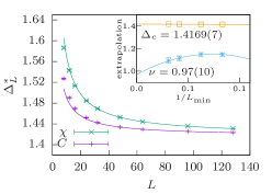
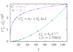
Figure 6: Finite-size scaling analysis in the second-order transition regime ($T=1.2$) based on the specific heat and magnetic susceptibility from data of the multicanonical simulations. Panel (a) shows a simultaneous fit of the pseudo-critical fields to the leading-order ansatz (16). The effective estimates are further subjected to an extrapolation in $1/L_{\mathrm{min}}$ as shown in the inset ($\Delta_{\rm eff}$ linear and $\nu_{\rm eff}$ quadratic in the lower-fit bound $1/L_{\rm min}$). Panel (b) shows fits of the maxima at the pseudo-critical points with the predicted behavior. The results verify the expected Ising universality class.

Correlation length:

We now turn to a discussion of the correlation length $\xi$. This is where we used the results of the hybrid method for improved precision. We determined the second-moment correlation length according to Eq. (11) and then used the quotient method to determine the limiting value of the ratio $\xi/L$ amit05 ; night ; bal96 ; fytas_PRL . We define a series of pseudo-critical points $\Delta_{(L,2L)}^{\ast}$ as the value of the crystal field where $\xi_{2L}/\xi_{L}=2$. These are the points where the curves of $\xi/L$ for the sizes $L$ and $2L$ cross. A typical illustration of this crossing is shown in the inset of Fig. 7(a) for $T=1.398$. The pair of system sizes considered is ($8$, $16$) and the results shown are obtained via both the hybrid method (data points) and the multicanonical approach through quasi continuous reweighting (lines). Denote the value of $\xi/L$ at these crossing points as $(\xi/L)^{\ast}$. The size evolution of $(\xi/L)^{\ast}$ and its extrapolation to the thermodynamic limit, denoted by $(\xi/L)_{\infty}$, will provide us with the desired test of universality. In Fig. 7(a) we illustrate the $L\rightarrow\infty$ extrapolation of $(\xi/L)^{\ast}$ for the previously studied case $T=1.398$ and compare the two simulation schemes, hybrid and multicanonical. The sequence of pairs of system sizes considered is as follows: ($8$, $16$), ($12$, $24$), ($16$, $32$), ($24$, $48$), ($32$, $64$), ($48$, $96$), and ($64$,$128$). It is seen that the results obtained with the hybrid method suffer less from statistical fluctuations. It is found that a second-order polynomial in $1/L$ describes the data for $(\xi/L)$ well and a corresponding fit yields

$$(\xi/L)_{\infty}^{\rm(hybrid)}=0.906(2).$$ (19)

A similar fitting attempt to the multicanonical data gives an estimate of

$$(\xi/L)_{\infty}^{\rm(muca)}=0.913(9),$$ (20)

consistent with but less accurate than $(\xi/L)_{\infty}^{\rm(hybrid)}$. Both estimates are fully consistent with the exact value $(\xi/L)_{\infty}=0.905\,048\,8292(4)$ salas2000 .

(a)                                                   (b)

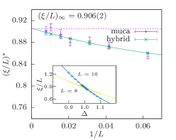
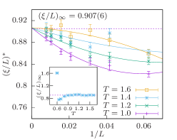
Figure 7: Finite-size scaling of the correlation length crossings $(\xi/L)^{\ast}$. The dashed horizontal line in both panels shows the asymptotic value for the square-lattice Ising model with periodic boundaries according to Eq. (4). (a) Results for $T=1.398$, comparing data from the multicanonical and hybrid methods. The line shows a quadratic fit in $1/L$ to the data from the hybrid method. The inset demonstrates the crossing point of $L=8$ and $L=16$ from both muca (lines) and hybrid (data points). (b) Simultaneous fit for several temperatures obtained from multicanonical simulations. The inset shows results from direct fits for a range of temperatures in comparison to the asymptotic value of Eq. (4). Well above the tricritical point, $(\xi/L)^{\ast}$ nicely converges towards the Ising value. Towards the tricritical point, additional corrections emerge.

In Fig. 7(b) we present a complementary illustration using data from the multicanonical approach and several temperatures in the second-order transition regime of the phase diagram, as indicated by the different colors. In particular, we show the values $(\xi/L)^{\ast}$ for several pairs of system sizes from ($8$, $16$) up to ($64$, $128$). The solid lines are second-order polynomial fits in $1/L$, imposing a common $L\rightarrow\infty$ extrapolation $(\xi/L)_{\infty}$. The result obtained in this way is $0.907(6)$, again well compatible with the exact Ising value. We note that following the discussion in Ref. salas2000 , a correction with exponent $1/L^{2}$ or possibly $1/L^{7/4}$ is expected, but a term proportional to $1/L$ is not. Here, however, we do not find consistent fits with $1/L^{7/4}$ or $1/L^{2}$ only, and using a second-order polynomial in $1/L^{w}$ instead we find $w=0.91(27)$, consistent with the two terms $1/L$ and $1/L^{2}$. A possible explanation for this behavior might be a non-linear dependence of the scaling fields on $L$ as a linear correction in reduced temperature $t$ produces a term $L^{-1/\nu}$ in FSS, and $\nu=1$ pelissetto2002 . In the inset of Fig. 7(b) we show the values of $(\xi/L)_{\infty}$ for various further temperatures. In this case, each estimate of $(\xi/L)_{\infty}$ is obtained from individual quadratic fits on each data set without imposing a common thermodynamic limit. The departure from the Ising value $0.905$, which is again marked by the dashed line, is clear as $T\rightarrow T_{\rm t}$. There, additional higher-order corrections due to the crossover to tricritical scaling become relevant.

Finally, we also considered the behavior of the susceptibility and specific heat from runs of the hybrid method, evaluated at the pseudo-critical points $\Delta_{(L,2L)}^{\ast}$ from the crossings of $\xi/L$. For $\chi$ we find an excellent fit for the full range of lattice sizes with the pure power-law form (18), resulting in $\gamma/\nu=1.75(2)$ ($Q=0.96$). Similarly, a fully consistent fit is found over the full lattice size range for the specific heat using the logarithmic form (17) ($Q=1.0$).

Full temperature range:

Having established the common first-order scaling for $T<T_{\rm t}$ and the Ising universality class for $T>T_{\rm t}$, we attempted to improve the precision in the location of the phase boundary for the square lattice model. To this end, we considered simultaneous fits of the scaling ansätze Eqs. (2) and (3) to the peak locations $\Delta^{\ast}_{L,C}$ and $\Delta^{\ast}_{L,\chi}$, depending on whether the considered temperature is in the first-order or in the second-order regime,

$$\Delta^{\ast}_{L,O} = \Delta^{\ast}+a_{O}L^{-D}\hskip 50.00008pt\text{for $T<T_{\rm t}$},$$ (21)

$$\Delta^{\ast}_{L,O} = \Delta_{\rm c}+a_{O}L^{-1/\nu}\hskip 45.00006pt\text{for $T>T_{\rm t}$},$$ (22)

with $D=2$ and $\nu=1$ fixed. As before, we take corrections to scaling into account by systematically omitting data from the small-$L$ side until fit qualities $Q>0.1$ are achieved. The results for the transition fields are listed in Table 1, including fit errors. Well inside the first-order regime, fits are excellent and cover the full data set ($L\geq 8$), so scaling corrections are not important there. Around the tricritical point, fits become difficult. For example, a simultaneous fit for $T=0.65$ with $L\geq 64$ still yields $Q\approx 0.07$. This is, of course, no surprise as we should see a crossover to the tricritical scaling there. Moving away from the tricritical point into the second-order regime, fits become more feasible. Corrections appear to be smallest between $T=0.9$ and $T=1.0$ where we could include the full data set, $L\geq 8$, with $Q\approx 0.4$ each. Increasing the temperature, we then again find stronger corrections. Particularly for $T=1.6$ fits with $L\geq 64$ are required to obtain $Q>0.1$. We attribute this effect to the fact that our variation of $\Delta$ is almost tangential to the phase boundary there, so field-mixing effects should be quite strong wilding1996 . Overall, we find very good agreement with recent previous studies, but often increased precision, cf. the data in Table 1.

Table 1: Representative points in the phase diagram of the Blume-Capel model on the square lattice from previous studies and the present work. In the first two columns we either indicate the value of $\Delta$ for simulations that vary $T$ or the value of $T$ for simulations that vary $\Delta$. Error bars are given in parenthesis in either $\Delta$ or $T$, depending on the simulation type.

		Beale		Silva et al.	Malakis et al.	Kwak et al.	This work
		Ref. beale1986		Ref. silva2006	Ref. malakis	Ref. kwak2015
$\Delta$	$T$	$\Delta$	$T$	$T$	$T$	$\Delta$	$\Delta$
0			1.695	1.714(2)	1.693(3)
	1.6						0.375(2)
	1.5						0.7101(5)
0.5			1.567	1.584(1)	1.564(3)
	1.4						0.9909(4)
	1.398						0.9958(4)
1.0			1.398	1.413(1)	1.398(2)
	1.3						1.2242(4)
	1.2						1.4167(2)
1.5			1.15	1.155(1)	1.151(1)
	1.1						1.5750(2)
	1.0						1.70258(7)
1.75					0.958(1)
	0.9						1.80280(6)
	0.8	1.87					1.87879(3)
1.9				0.755(3)	0.769(1)
	0.7	1.92					1.93296(2)
1.95				0.651(2)	0.659(2)
	0.65	1.95				1.9534 (1)	1.95273(1)
	0.61	1.9655
	0.608					1.96604 (1)
	0.6	1.969				1.96825 (1)	1.968174(3)
1.975					0.574(2)
1.992				0.499(3)
	0.5	1.992				1.98789 (1)	1.987889(5)
	0.4					1.99681 (1)	1.99683(2)

5 Summary and outlook

In this paper we have reviewed and extended the phase diagram of the 2D Blume-Capel model in the absence of an external field, providing extensive numerical results for the model on the square lattice. In particular, we studied in some detail the universal ratio $\xi/L$ that allows to confirm the Ising universality class of the model in the second-order regime of the phase boundary. In contrast to most previous work, we focused on crossing the phase boundary at constant temperature by varying the crystal field $\Delta$ zierenberg2015 . Employing a multicanonical scheme in $\Delta$ allowed us to get results as continuous functions of $\Delta$ and to overcome the free-energy barrier in the first-order regime of transitions. A finite-size scaling analysis based on a specific-heat-like quantity and the magnetic susceptibility provided us with precise estimates for the transition points in both regimes of the phase diagram that compare very well to the most accurate estimates of the current literature. We have been able to probe the first-order nature of the transition in the low-temperature phase and to illustrate the Ising universality class in the second-order regime of the phase diagram. We are also able to provide accurate estimates of the critical exponents $\nu$ and $\gamma/\nu$, as well as to clearly confirm the logarithmic divergence of the specific-heat peaks. Using additional simulations based on a hybrid cluster-update approach we studied the correlation length in the second-order regime. Via a detailed scaling analysis of the universal ratio $\xi/L$, we could show that it cleanly approaches the value $(\xi/L)_{\infty}=0.905\ldots$ of the Ising universality class for all temperatures up to the tricritical point.

In the first-order regime we found a somewhat surprising $1/L$ correction in the scaling of the conventional susceptibility defined according to Eq. (10). As it turns out, this is due to the explicit symmetry breaking by using $|M|$ instead of $M$ in the definition of $\chi$. For a modified symmetry breaking prescription that leaves the disordered peak invariant, this correction disappears. It would be interesting to see whether similar corrections are found in other systems with first-order transitions, such as the Potts model.

To conclude, the Blume-Capel model serves as an extremely useful prototype system for the study of phase transitions, exhibiting lines of second-order and first-order transitions that meet in a tricritical point. Apart from the interest in tricritical scaling, this model hence also allows to investigate the effect of disorder on phase transitions of different order within the same model. A study of the disordered version of the model is thus hoped to shed some light on questions of universality between the continuous transitions in the disordered case that correspond to different transition orders in the pure model fytas_PRE .

- (1) M. Blume, Phys. Rev. 141, 517 (1966)
- (2) H.W. Capel, Physica (Utr.) 32, 966 (1966); H.W. Capel, Physica (Utr.) 33, 295 (1967); H.W. Capel, Physica (Utr.) 37, 423 (1967)
- (3) I.D. Lawrie, S. Sarbach, in: C. Domb, J.L. Lebowitz (Eds.), Phase Transitions and Critical Phenomena, Vol. 9 (Academic Press, London, 1984)
- (4) W. Selke, J. Oitmaa, J. Phys. C 22, 076004 (2010)
- (5) N.G. Fytas, Eur. Phys. J. B 79, 21 (2011)
- (6) J. Zierenberg, N.G. Fytas, W. Janke, Phys. Rev. E 91, 032126 (2015)
- (7) A.N. Berker, M. Wortis, Phys. Rev. B 14, 4946 (1976)
- (8) D.P. Landau, Phys. Rev. Lett. 28, 449 (1972)
- (9) M. Kaufman, R.B. Griffiths, J.M. Yeomans, M. Fisher, Phys. Rev. B 23, 3448 (1981)
- (10) W. Selke, J. Yeomans, J. Phys. A 16, 2789 (1983)
- (11) W. Selke, D.A. Huse, D.M. Kroll, J. Phys. A 17, 3019 (1984)
- (12) D.P. Landau, R.H. Swendsen, Phys. Rev. B 33, 7700 (1986)
- (13) J.C. Xavier, F.C. Alcaraz, D. Pena Lara, J.A. Plascak, Phys. Rev. B 57, 11575 (1998)
- (14) Y. Deng, W. Guo, H.W.J. Blöte, Phys. Rev. E 72, 016101 (2005)
- (15) C.J. Silva, A.A. Caparica, J.A. Plascak, Phys. Rev. E 73, 036702 (2006)
- (16) D. Hurt, M. Eitzel, R.T. Scalettar, G.G. Batrouni, in: Computer Simulation Studies in Condensed Matter Physics XVII, Springer Proceedings in Physics, Vol. 105, eds. D.P. Landau, S.P. Lewis, H.-B. Schüttler (Springer, Berlin, 2007)
- (17) A. Malakis, A.N. Berker, I.A. Hadjiagapiou, N.G. Fytas, Phys. Rev. E 79, 011125 (2009); A. Malakis, A.N. Berker, I.A. Hadjiagapiou, N.G. Fytas, T. Papakonstantinou, Phys. Rev. E 81, 041113 (2010)
- (18) W. Kwak, J. Jeong, J. Lee, D.-H. Kim, Phys. Rev. E 92, 022134 (2015)
- (19) M.J. Stephen, J.L. McColey, Phys. Rev. Lett. 44, 89 (1973)
- (20) T.S. Chang, G.F. Tuthill, H.E. Stanley, Phys. Rev. B 9, 4482 (1974)
- (21) G.F. Tuthill, J.F. Nicoll, H.E. Stanley, Phys. Rev. B 11, 4579 (1975)
- (22) F.J. Wegner, Phys. Lett. 54A, 1 (1975)
- (23) P.F. Fox, A.J. Guttmann, J. Phys. C 6, 913 (1973)
- (24) W.J. Camp, J.P. Van Dyke, Phys. Rev. B 11, 2579 (1975)
- (25) T.W. Burkhardt, R.H. Swendsen, Phys. Rev. B 13, 3071 (1976)
- (26) P.D. Beale, Phys. Rev. B 33, 1717 (1986)
- (27) T.W. Burkhardt, Phys. Rev. B 14, 1196 (1976)
- (28) T.W. Burkhardt, H.J.F. Knops, Phys. Rev. B. 15, 1602 (1977)
- (29) M. Kaufman, R.B. Griffiths, J.M. Yeomans, M.E. Fisher, Phys. Rev. B 23, 3448 (1981)
- (30) J.M. Yeomans, M.E. Fisher, Phys. Rev. B 24, 2825 (1981)
- (31) N.B. Wilding, P. Nielaba, Phys. Rev. E 53, 926 (1996)
- (32) J.A. Plascak, P.H.L. Martins, Comput. Phys. Commun. 184, 259 (2013)
- (33) K. Binder, D.P. Landau, Phys. Rev. B 30, 1477 (1984); M.S.S. Challa, D.P. Landau, K. Binder, Phys. Rev. B 34, 1841 (1986)
- (34) W. Janke, First-Order Phase Transitions, in: Computer Simulations of Surfaces and Interfaces, NATO Science Series, II. Mathematics, Physics and Chemistry - Vol. 114, Proceedings of the NATO Advanced Study Institute, Albena, Bulgaria, 9–20 September 2002, eds. B. Dünweg, D.P. Landau, A.I. Milchev (Kluwer, Dordrecht, 2003), pp. 111–135; W. Janke, R. Villanova, Nucl. Phys. B 489, 679 (1997)
- (35) D.P. Landau, K. Binder, Monte Carlo Simulations in Statistical Physics (Cambridge University Press, Cambridge, 2000)
- (36) J. Cardy, Scaling and Renormalization in Statistical Physics (Cambridge University Press, Cambridge, 1996)
- (37) A. Pelissetto and E. Vicari, Phys. Rep. 368, 549 (2002)
- (38) J. Salas, A.D. Sokal, J. Stat. Phys. 98, 551 (2000)
- (39) W. Selke, L.N. Shchur, J. Phys. A 38, L739 (2005)
- (40) B.A. Berg, T. Neuhaus, Phys. Lett. B 267, 249 (1991); B.A. Berg, T. Neuhaus, Phys. Rev. Lett. 68, 9 (1992)
- (41) W. Janke, Int. J. Mod. Phys. C 03, 1137 (1992); W. Janke, Physica A 254, 164 (1998)
- (42) J. Zierenberg, M. Marenz, W. Janke, Comput. Phys. Comm. 184, 1155 (2013); J. Zierenberg, M. Marenz, W. Janke, Physics Procedia 53, 55 (2014)
- (43) C.M. Fortuin, P.W. Kasteleyn, Physica 57, 536 (1972)
- (44) R.H. Swendsen and J.S. Wang, Phys. Rev. Lett. 58, 86 (1987)
- (45) H.W.J. Blöte, E. Luijten, J.R. Heringa, J. Phys. A: Math. Gen. 28, 6289 (1995)
- (46) M. Hasenbusch Phys. Rev. B 82, 174433 (2010)
- (47) A. Malakis, A.N. Berker, N.G. Fytas, T. Papakonstantinou, Phys. Rev. E 85, 061106 (2012)
- (48) U. Wolff, Phys. Rev. Lett. 62, 361 (1989)
- (49) B. Efron, The Jackknife, the Bootstrap and other Resampling Plans (Society for Industrial and Applied Mathematics, Philadelphia, 1982); B. Efron, R.J. Tibshirani, An Introduction to the Bootstrap (Chapman and Hall, Boca Raton, 1994)
- (50) F. Cooper, B. Freedman, D. Preston, Nucl. Phys. B 210, 210 (1982)
- (51) H.G. Ballesteros, L.A. Fernández, V. Martín-Mayor, A. Muñoz Sudupe, G. Parisi, J.J. Ruiz-Lorenzo, J. Phys. A: Math. Gen. 32, 1 (1999)
- (52) P. Young, Everything You Wanted to Know About Data Analysis and Fitting but Were Afraid to Ask, SpringerBriefs in Physics (Springer, Berlin, 2015)
- (53) D. Amit, V. Martín-Mayor, Field Theory, the Renormalization Group and Critical Phenomena, 3rd edition (World Scientific, Singapore, 2005)
- (54) M.P. Nightingale, Physica (Amsterdam) 83A, 561 (1976)
- (55) H.G. Ballesteros, L.A. Fernández, V. Martín-Mayor, A. Muñoz-Sudupe, Phys. Lett. B 378, 207 (1996)
- (56) N.G. Fytas, V. Martín-Mayor, Phys. Rev. Lett. 110, 227201 (2013)
- (57) P.E. Theodorakis, N.G. Fytas, Phys. Rev. E 86, 011140 (2012)