The [Ne iii] Jet of DG Tau and Its Ionization Scenarios

Abstract

Forbidden neon emission from jets of low-mass young stars can be used to probe the underlying high-energy processes in these systems. We analyze spectra of the jet of DG Tau obtained with the Very Large Telescope/X-Shooter spectrograph in 2010. [Ne iii] $\lambda 3869$ is clearly detected in the innermost 3″ microjet and the outer knot located at $\sim 6\farcs 5$. The velocity structure of the inner microjet can be decomposed into the low-velocity component (LVC) at $\sim-70$ km s^-1 and the high-velocity component (HVC) at $\sim-180$ km s^-1. Based on the observed [Ne iii] flux and its spatial extent, we suggest the origins of the [Ne iii] emission regions and their relation with known X-ray sources along the jet. The flares from the hard X-ray source close to the star may be the main ionization source of the innermost microjet. The fainter soft X-ray source at $0\farcs 2$ from the star may provide sufficient heating to help to sustain the ionization fraction against the recombination in the flow. The outer knot may be reionized by shocks faster than 100 km s^-1 such that [Ne iii] emission reappears and that the soft X-ray emission at $5\farcs 5$ is produced. Velocity decomposition of the archival Hubble Space Telescope spectra obtained in 1999 shows that the HVC had been faster, with a velocity centroid of $\sim-260$ km s^-1. Such a decrease in velocity may potentially be explained by the expansion of the stellar magnetosphere, changing the truncation radius and thus the launching speed of the jet. The energy released by magnetic reconnections during relaxation of the transition can heat the gas up to several tens of megakelvin and provide the explanation for on-source keV X-ray flares that ionize the neon microjet.

1 INTRODUCTION

Observations of kinematic structures and physical conditions of jets and winds from young stellar objects (YSOs) help to clarify how outflows regulate the formation of young stars. Spectroscopic studies of forbidden optical emission lines from classical T Tauri stars (TTSs) provide diagnostics of both kinematic and physical properties of the jets and their driving region (Reipurth & Bally, 2001). Spatially resolved spectroscopy (Bacciotti et al., 2000; Coffey et al., 2008) of low-excitation, high-abundance line species such as [O i], [S ii], and [N ii] has been used to deduce physical conditions and kinematic properties along the jet.

Forbidden lines of singly and doubly ionized neon provide useful diagnostics of the physical conditions around the young stars (Glassgold et al., 2007; Hollenbach & Gorti, 2009) because of the high ionization potentials of neon. The 12.81µm  [Ne ii] fine-structure line has been detected toward low-mass YSOs associated with X-ray/ultraviolet photoevaporating disks (Pascucci & Sterzik, 2009), and in the terminal knots of jets and outflows from low-mass protostars (van Boekel et al., 2009). Photoionization by keV X-ray photons may be an important source of [Ne ii] excitation in disk atmospheres (Glassgold et al., 2007) and in jets and outflows (Shang et al., 2010). With a large critical density ($n_{\rm cr}\sim 10^{7}$ cm^-3 at $T\sim 10^{4}$ K), the optical forbidden [Ne iii] $\lambda 3869$Å transition has been used as a marker for high-energy photons or for strong shocks in studies of high-mass star formation and active galactic nuclei. Among the low-mass YSOs, detections of [Ne iii] $\lambda 3869$ close to the central star have been reported recently (on the scale of arcseconds), mainly associated with their jets (Liu et al., 2014; Whelan et al., 2014).

DG Tau, located in the Taurus–Auriga molecular cloud at a distance of $\sim$140 pc (Kenyon et al., 1994; Torres et al., 2007), is an actively accreting extreme T Tauri star with a spectrum consistent with a heavily veiled $\sim$K7 star (Herczeg & Hillenbrand, 2014). The flat spectral energy distribution in the near- to mid-infrared (Kenyon & Hartmann, 1995; Hartmann et al., 2005) suggests that DG Tau may represent a transition stage between the Class I and Class II YSOs. The high optical veiling prevents an accurate determination of the extinction (Hartigan et al., 1995; Gullbring et al., 1998; White & Hillenbrand, 2004; Herczeg & Hillenbrand, 2014). From modeling ultraviolet to optical continuum, Gullbring et al. (2000) estimated a mass accretion rate of $\dot{M}_{\rm acc}\sim 5\times 10^{-7}M_{\odot}\,\rm{yr^{-1}}$ with a moderate extinction of $A_{V}\approx 1.6$ (a value independently obtained through spectral typing by Herczeg & Hillenbrand, 2014). The bright [O i] and [S ii] emission is consistent with a strong outflow (Hartigan et al., 1995; White & Hillenbrand, 2004); using $A_{V}\approx 1.6$, a mass-loss rate $\dot{M}_{\rm w}\gtrsim 1\times 10^{-7}M_{\odot}\,{\rm yr}^{-1}$ was deduced using the [O i] flux obtained by Hartigan et al. (1995).

DG Tau drives an optically visible jet at a position angle of $\sim 226\arcdeg$. Optical spectra have revealed it to be blueshifted (Solf & Böhm, 1993). From the proper motion of the knots 5″-10″ from the star, an inclination angle of $37\fdg 7\pm 2\arcdeg$ with respect to the line of sight has been inferred (Eislöffel & Mundt, 1998). The inner 5″ of the jet has been mapped using broad-band optical imaging with the Hubble Space Telescope (HST) (Stapelfeldt et al., 1997) and using adaptive optics (AO)-aided narrow-band imaging from the Canada-France-Hawai‘i Telescope (CFHT) (Dougados et al., 2000). Both images showed a jet-like structure within 2″ of the source, and an emission peak at around 4″ that resembles a bow shock. Using CFHT integral-field spectroscopy to investigate the kinematics at spatial scales smaller than 5″, Lavalley-Fouquet et al. (2000) showed that the jet-like feature reaches its highest velocity of $\sim-350$ km s^-1 at $\sim 1\farcs 3$ and drops to $\sim-280$ km s^-1 afterwards, before approaching $\sim-260$ km s^-1 at the 4″ bow shock. Lower-velocity material ($\lesssim-100$ km s^-1) appears to have a larger transverse spatial extent and is concentrated closer to the star. The two distinct kinematic features and their spatial and morphological differences have been further traced to within 2″ with HST/Space Telescope Imaging Spectrograph (STIS) in optical forbidden lines (Bacciotti et al., 2000, 2002) and with the Subaru Telescope in the near-infrared 1.644µm [Fe ii] line (Pyo et al., 2003).

The region of the innermost few arcseconds of the jet, often dubbed the “microjet” (Solf, 1997), reveals information close to the jet-driving source. HST/STIS spectra provide an opportunity to probe the kinematics of the DG Tau microjet at $\sim 0\farcs 1$ spatial resolution. Bacciotti et al. (2000) constructed channel maps of H$\alpha$ and optical forbidden emission lines from these spectra. They binned spectra with velocities between $+70$ and $-420$ km s^-1 into four distinct velocity channels of approximately 125 km s^-1 width. The channels were designated as low-, medium-, high-, and very-high-velocity, respectively, indicating increasingly blueshifted radial velocities. Within 0$\farcs$7 of the star, the outflow has the form of a collimated jet. This is most evident in the high-velocity channel. A bubble-like feature, most evident at intermediate velocities, is seen between 0$\farcs$4 and 1$\farcs$5 from the star. Maurri et al. (2014) inferred physical conditions such as temperature and density along and across the jet from line ratios. The blueshifted jet was found to have a high density of $n_{\rm H}\sim 3\times 10^{6}$ cm^-3 and low electron fraction $x_{e}\sim 0.03$ and to reach an order-of-magnitude lower density and a high electron fraction of 0.7 at $\sim 0\farcs 7$ and around $2\arcsec$ from the jet source. On the other hand, the physical conditions were found to alter little across the jet. This spatial variations in physical conditions were interpreted as arising from ionization with shocks weaker than $\sim 100$ km s^-1.

DG Tau is an active and bright X-ray source. It is the first known low-mass YSO to show spatially resolved X-ray emission along the jet axis, extending up to 5″ from the star (Güdel et al., 2005, 2008). The extended X-rays have a luminosity of $\sim 10^{28}$ erg s^-1 and plasma temperature of $\sim 3$ MK (Güdel et al., 2008). It exhibits a proper motion of $\sim 0\farcs 3\,{\rm yr}^{-1}$, similar to other optical and infrared knots, leading to its identification as an “X-ray jet” (Güdel et al., 2012; Rodríguez et al., 2012). The on-source X-ray emission consists of a hard, flaring component with $L_{\rm X}\sim 10^{30}$ erg s^-1 and $T_{\rm X}\sim 30$ MK and a soft, steadier component with $L_{\rm X}$ and $T_{\rm X}$ roughly an order of magnitude lower than those of the hard component (Güdel et al., 2008). Multi-year Chandra observations show that the hard component is located at the stellar position and the soft component is offset along the optical jet axis by 0$\farcs$2 (Schneider & Schmitt, 2008). The flaring hard component is attributed to the coronal emission common to YSOs; its inferred column density of $N_{\rm H}\sim$ 2–3$\times 10^{22}$ cm^-2 (corresponding to $A_{V}=N_{\rm H}/2\times 10^{21}\approx$ 10–15, Vuong et al., 2003) is much higher than the value ($A_{V}\approx 1.6$ or $N_{\rm H}\approx 3\times 10^{21}$ cm^-2) obtained from optical-to-infrared photometry. The soft near-source component has a spectrum similar to that of the extended X-ray jet and a lower column density $N_{\rm H}\sim 1.1\times 10^{21}$ cm^-2, corresponding to $A_{V}\approx 0.55$ (Güdel et al., 2008, 2012). It may be associated with an inner part of the jet. Spatially resolved HST spectra in the far-ultraviolet (FUV) C iv doublet show the visual proximity between the C iv emission and the off-source soft X-ray component. This spatial correlation may suggest local heating up to $10^{5}$ K along the path of propagation of the jet (Schneider et al., 2013a, b). Understanding the roles of these multiple X-ray components associated with the jet can help to elucidate the ionization and excitation of the jet upon launching and during propagation.

In this paper, we present spatially resolved spectroscopy of DG Tau’s jet observed with HST/STIS in 1999 and VLT/X-Shooter in 2010. In both spectra we identify double velocity components from the observed line profiles. In the X-Shooter spectra, [Ne iii] $\lambda 3869$ traces the jet up to 8″ from the star, with double velocity components within the inner 3″. In Section 2, we present the observations and analysis of the two data sets. In Section 3, we describe the properties of the decomposed spectra, and the properties of the [Ne iii] jet. Possible origins of the [Ne iii] emission in the DG Tau jet is discussed in Section 4 and the evolution of the velocity components during the two observation epochs are discussed in Section 5. We summarize our findings in Section 6.

2 Observations and Analysis

2.1 HST/STIS Archival Data Analysis

Figure 1: The inner 2″ PV diagrams of the DG Tau jet obtained by averaging the HST/STIS spectra from seven slit positions perpendicular to the jet. The emission lines of [O i] $\lambda 6363$, [S ii] $\lambda 6731$, and [N ii] $\lambda 6583$, are shown from left to right. The contours are logarithmic with $\sqrt{2}\sigma$ increments, starting from $10\sigma$. The $1\sigma$ uncertainties for [O i], [S ii], and [N ii] are $2.8\times 10^{-16}$, $2.4\times 10^{-16}$, and $2.2\times 10^{-16}$ erg s^-1 cm^-2 arcsec^-2, respectively. The line profiles at each spatial position have been fitted and decomposed into two Gaussian profiles. The fitted velocity centroids of the decomposed profiles are shown by squares and diamonds for the high-velocity and low-velocity components, respectively. The filled and open symbols represent the stronger and weaker velocity components at each spatial position.

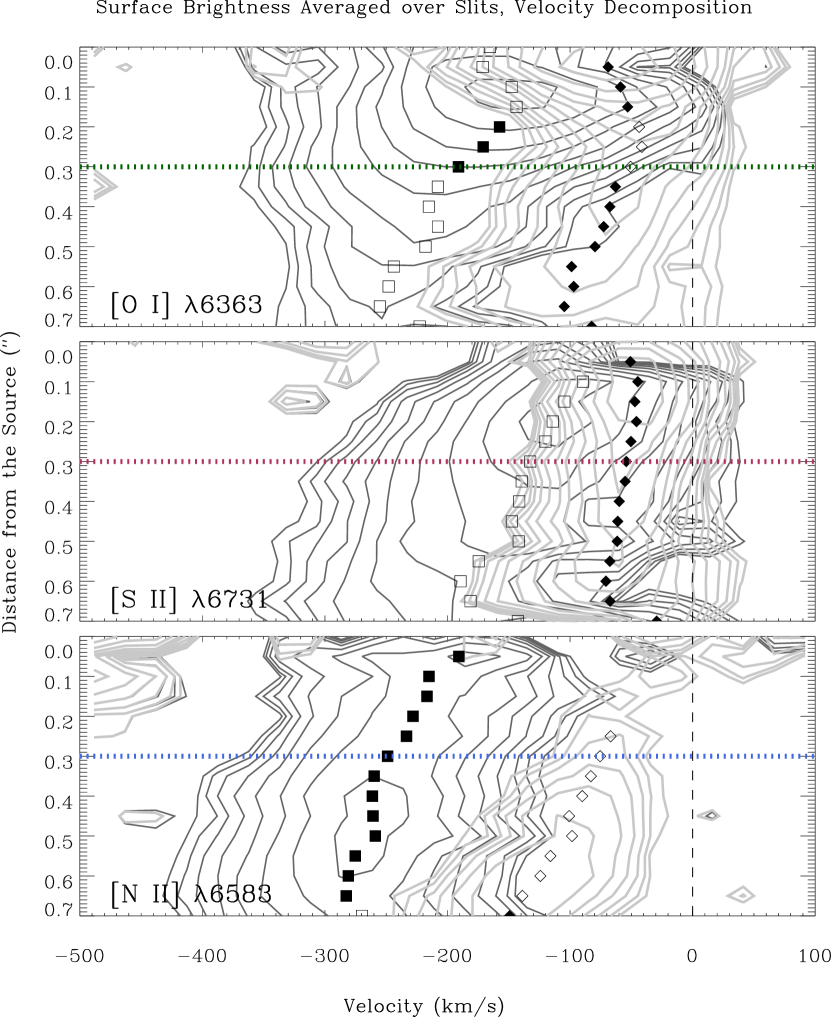
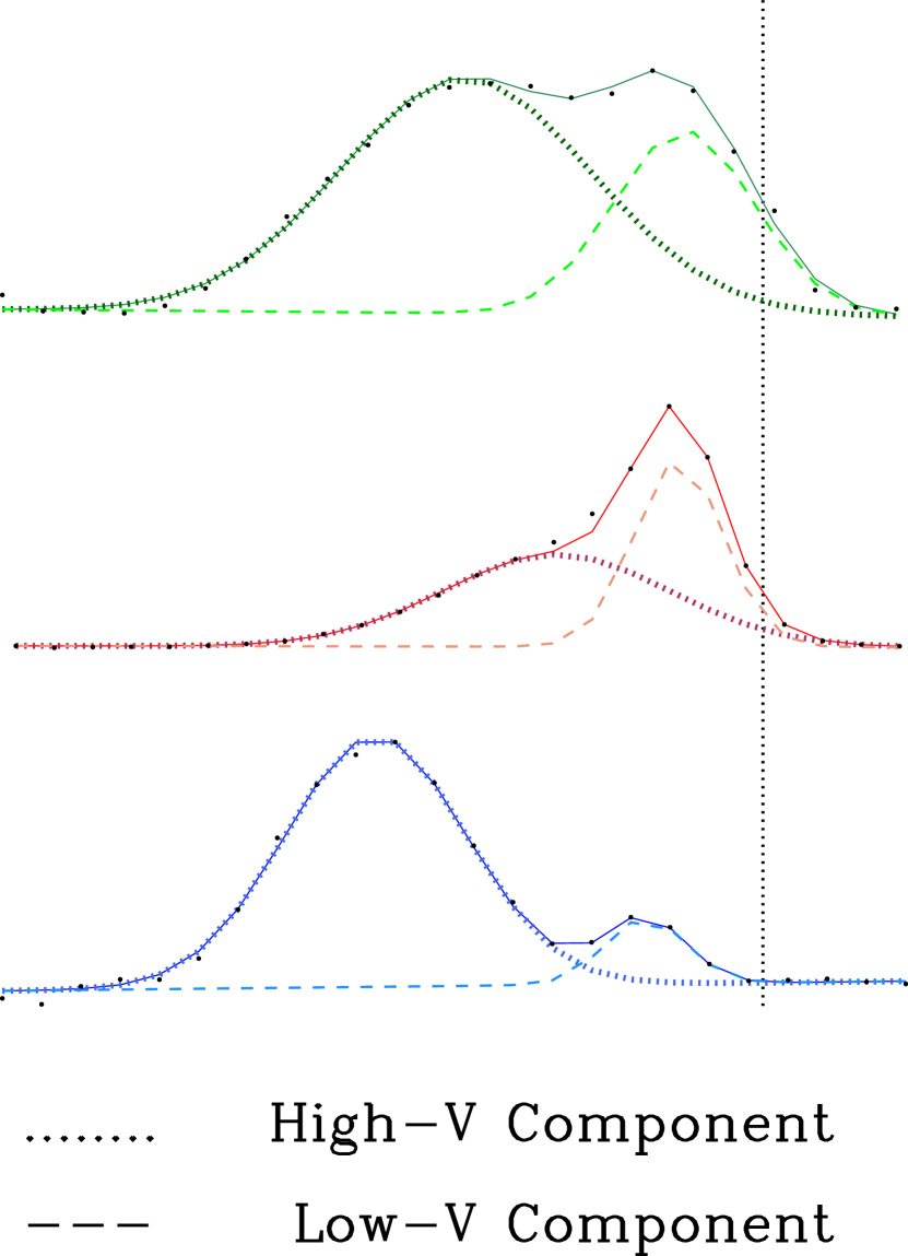
Figure 2: The inner 0$\farcs$7 PV diagrams made by averaging the HST/STIS spectra from seven slit positions, showing those of [O i] $\lambda 6363$, [S ii] $\lambda 6731$, and [N ii] $\lambda 6583$, from top to bottom. The contours are logarithmic with $\sqrt{2}\sigma$ increments, starting from $10\sigma$. The $1\sigma$ uncertainties for [O i], [S ii], and [N ii] are $3.5\times 10^{-16}$, $3.4\times 10^{-16}$, and $2.0\times 10^{-16}$ erg s^-1 cm^-2 arcsec^-2, respectively. The line profiles are decomposed into a higher (black contours) and a lower (gray contours) velocity component with two Gaussians. The right panels show the observed line profiles (discrete points) and the two-Gaussian fits at a position of 0$\farcs$3 to illustrate the concept of velocity decomposition. The overall (summed) line profiles are shown by thin solid lines. The fitted HVC profiles are shown by thick dashed Gaussians and the fitted LVC profile are shown edit2by thin dashed Gaussians. The centroids from two-Gaussian fitting are plotted with squares (the lower velocity Gaussian) and diamonds (the higher velocity Gaussian) are plotted on top of the contours in the left panels. The filled symbols show the Gaussian with higher intensity and open symbols the Gaussian with lower intensity. The results indicate the different nature of the three lines, with the [O i] and [S ii] lines dominating at low velocity ($<200$ km s^-1) before 0$\farcs$7, and the [N ii] line peaking at high velocity ($\sim 260$ km s^-1) throughout the flow.

We downloaded pipeline-processed DG Tau spectra of the HST Cycle 7 observations from the Mikulski Archive for Space Telescopes (MAST). The observations were taken on 1999 January 14 (GO 7311, PI: R. Mundt) with the STIS. The observational settings have been described by Bacciotti et al. (2000) and Maurri et al. (2014), so we summarize only the essential properties here. The $\mathtt{52\times 0.1}$ slit and G750M grating centered at 6581Å were used to cover six bright optical forbidden emission lines and H$\alpha$. Seven slit positions parallel to the axis of the DG Tau jet (P.A.$=226\arcdeg$) were observed, each offset by 0$\farcs$07 in the transverse direction to cover a total span of 0$\farcs$52 across the jet. Each exposure yielded a two-dimensional spectral image covering 52″ (0$\farcs$05 pixel^-1 or $\sim 0\farcs 1$ FWHM) perpendicular to the jet, and 6295–6867 Å along the dispersion axis (0.554Å pixel^-1, corresponding to $\sim 25$ km s^-1), with a velocity resolution of $\sim 65$ km s^-1.

The pipeline-processed spectra from MAST suffice for data analysis. Hot pixels were present primarily in the line-free regions. Bad pixels that affect a few rows of the spectra between 1″ and 2″  were flagged by inspection. Further reductions primarily consisted of removing the stellar continuum and the contribution from the reflecting nebula. Each spectral image was first divided into three sub-images containing lines of [O i], H$\alpha+$[N ii], and [S ii], respectively. On each sub-image, the rows containing the blueshifted jet extending up to 2″ from the star were examined to remove the semi-periodic baseline undulations resulting from wavelength rectification of the undersampled star. To each row, we fit and subtract the baseline with a Legendre polynomial up to the tenth order, depending on the distance to the star. The tasks were performed within IRAF/STSDAS GFIT1D using the amoeba $\chi^{2}$ minimization.

We extracted position–velocity (PV) diagrams for [O i] $\lambda\lambda 6300/6363$, [N ii] $\lambda\lambda 6548/6583$, and [S ii] $\lambda\lambda 6717/6731$. We converted wavelengths to radial velocities, assuming the systemic velocity of DG Tau to be $+16.5$ km s^-1 (Bacciotti et al., 2000). PV diagrams were extracted from each of the seven slit positions, and also from transversely averaged spectral images to cover the emission across the jet and raise the signal-to-noise ratio. PV diagrams of the jet up to $-500$ km s^-1 can be extracted, except for [O i] $\lambda 6300$, which is cut off at $\sim-230$ km s^-1 by the end of the detector. We therefore used [O i] $\lambda 6363$ for kinematic studies of the [O i] emission whenever applicable. Figure 1 shows the baseline-subtracted PV diagrams for the innermost 2″ of the jet, averaged over the seven slits across 0$\farcs$52 perpendicular to the jet axis. [O i] $\lambda 6363$, [S ii] $\lambda 6731$, and [N ii] $\lambda 6583$ are shown.

Astrophysical emission lines are generally not Gaussian, but, where appropriate, single Gaussian fits do provide robust estimates of the bulk velocity (the line centroid) and the line broadening. Visual inspection of the PV diagrams shows that single Gaussians often do not suffice to describe the observed line profiles, so we decomposed the spectra into different velocity components by fitting two independent Gaussian profiles every 0$\farcs$05. These line profiles can appear double-peaked, flat-topped, or skewed, depending on the relative fluxes of gases at different velocities. This can be visualized through the V-shaped isocontours in the PV diagrams for the innermost 1″ of the jet (Figure 1), which is suggestive of double velocity components. Indeed, it has long been known that double velocity components exist in the DG Tau jet (Solf & Böhm, 1993; Pyo et al., 2003). While the fitting and the decomposition are a mathematical exercise, the component centroids and widths constrain the true physical velocity distributions of the gas. Where two distinct Gaussian components are mathematically required, we interpret the two components as distinct regions at different bulk velocities. The variations of these principal velocity components with position along the jet can be either continuous or abrupt depending on the propagation history of the jet. The relative fluxes of these principal velocity components may also change along the flow. These variations provide insights into the ejection history and possible variations of properties close to the jet launching region.

We used the IRAF/STSDAS NGAUSSFIT task to interactively give initial guesses for the Gaussian parameters and then recursively minimized $\chi^{2}$ with the amoeba algorithm. The concept of velocity decomposition and the resulting decomposed PV diagrams of the DG Tau microjet within 0$\farcs$7 from the star are shown in Figure 2. [O i] $\lambda 6363$, [S ii] $\lambda 6731$, and [N ii] $\lambda 6583$ are shown, along with their line profiles at 0$\farcs$3 to show the representative decompositions using two-Gaussian fitting.

2.2 VLT/X-Shooter Optical Spectra

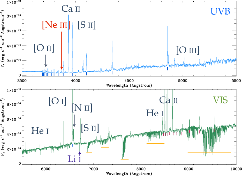
Figure 3: One-dimensional spectra of DG Tau from the UVB (top) and VIS (bottom) arms by summing over $\pm 3\arcsec$ from the stellar position. The blue vertical bars show the identifications of the Balmer series and the red vertical bars show the Paschen series. The spectra were not corrected for telluric absorption; regions dominated by telluric absorption are marked with yellow horizontal bars. Other bright permitted lines (He i and Ca ii) and forbidden lines ([O i], [O ii], [O iii], [S ii], [N ii]) are labeled. The location of [Ne iii] $\lambda 3869$ is shown in red in the top panel.

New long-slit spectra of DG Tau and its jets were obtained with the X-Shooter spectrograph on the Very Large Telescope (VLT) on 2010 January 19 (084.C-1095(A), PI: G. Herczeg). A spatial coverage of 21″ was obtained by using an 11″ long slit in the nodding mode with two nodding positions separated by 10″ at the position angle of 227°, roughly along the jet axis. An ABBA nodding pattern was used. The three spectral arms simultaneously cover the UVB (300–550 nm), VIS (550–1000 nm), and NIR (1000–2500 nm) ranges, with pixel scales of 0$\farcs$2 pixel^-1 in the spatial direction and 0.02 nm pixel^-1 in the dispersion direction ($\sim 15$, $8$, and $4$ km s^-1 for the three arms, respectively). Exposure times for each nodding position were 240, 250, and 15 s for the three arms, respectively. Slit widths of 1$\farcs$3, 1$\farcs$2, and 1$\farcs$2 were used for the three arms, respectively, resulting in a spectral resolution of $R\sim 5000$ ($\Delta v\sim 60$ km s^-1). The seeing was $\sim 1\arcsec$ throughout the observation and within the observed spectral range.

We confine our reduction and analysis to the UVB and VIS arms. The spectra were reduced with the X-Shooter pipeline version 2.4.0 using the EsoRex version 3.10.2. The reduction cascade of the stare mode was adopted instead of the nodding mode, since both nodding positions were used as the source frame. In the pipeline, bias and dark subtraction, flat-fielding, wavelength calibration, sky subtraction, and flux calibration were performed and two-dimensional spectra were obtained after concatenating adjacent orders. Two exposures of the same nodding positions were combined during the reduction cascade, and the combined data of the two nodding positions were connected by matching the spectrally summed spatial profiles along the jet axis. The resulting spectra contain the first $\sim 14\farcs 2$ of the blueshifted jet and $\sim 6\farcs 8$ of the redshifted counterjet. Median filters were used to remove the remaining hot and bad pixels to produce the final flux-calibrated and sky-subtracted two-dimensional spectral images. Figure 3 shows the reduced one-dimensional spectrum of DG Tau and its microjet, extracted within $\pm 3\arcsec$ of the jet axis. Li i $\lambda 6707$ is detected at 6708.8 Å, at a velocity shift of $+43.1$ km s^-1, which we adopted as the systemic velocity offset for this data set.

To extract line properties, we removed the continuum emission in the spectra by fitting the line-free regions with polynomials. The combined spectra were first divided into segments of spectral ranges. Most of the segments follow spectral orders, except for the regions between 700–800 nm and between 900–1000 nm in the VIS arm, in which two orders were combined to cover telluric absorption features. In each segment, line-free regions were selected by consecutive moving median filters of increasing box sizes and fine-tuned by cross-checking with the emission line database and by inspection. The fitting and subtraction were performed at each row along the slit; the order of the polynomial was varied from 3 to 7 depending on the emission features in the individual row.

PV diagrams were created from the continuum-subtracted two-dimensional spectra. Two-Gaussian velocity decomposition was performed as described in Section 2.1. Selected PV diagrams of emission lines from the UVB and VIS arms are shown in Figures 4 and 5, respectively. The fitted velocity centroids are overlaid on the PV diagrams and are further described in Section 3.2.

3 RESULTS

3.1 Kinematics of the Microjet from Archival HST/STIS Spectra

Using the archival HST/STIS spectra taken in 1999, we obtained PV diagrams of the blueshifted microjet of DG Tau covering positions within 2″ of the star (Figure 1). In this figure, the velocity centroids measured by two-Gaussian decomposition are overlaid on the PV diagrams, with the squares representing the centroids of the high-velocity component (HVC) and the diamonds representing those of the low-velocity component (LVC). At each spatial position, the stronger component is rendered with the filled symbol and the weaker component with the open symbol. Where a single Gaussian fit suffices (as at distances 0$\farcs$75–0$\farcs$95 and 1$\farcs$0–1$\farcs$6 in the [O i] and [N ii] PV plots), the filled square symbols represent the sole velocity.

Three kinematic regions are evident within the innermost 2″. The first region, from the star out to $\sim 0\farcs 7$, is characterized by a smooth change in velocity centroids. This we regarded as the innermost undisturbed microjet. The second region starts from $\sim 0\farcs 7$, where a velocity discontinuity is seen in both the HVC and LVC. Spatially, this coincides with the A2 region identified in the literature (Bacciotti et al., 2000; Maurri et al., 2014). Within this region, the HVC and LVC centroids of [O i] and [S ii] emission decrease by $\sim 100$ and $\sim 50$ km s^-1, respectively; on the other hand, the two components of [N ii] seems to merge. Another discontinuity from $\sim-200$ km s^-1 to $\sim-350$ km s^-1 marks the start of the third region. In the [O i] and [N ii] lines, the velocity jump occurs at $\sim 1\arcsec$; this change appears to occur about 0$\farcs$2 further out in [S ii]. For all the lines, the emission peaks at $\sim 1\farcs 35$ with a velocity centroid of $\sim-360$ km s^-1and then becomes fainter and less ordered downstream. This region coincides with A1 (Bacciotti et al., 2000; Maurri et al., 2014). Table 1 shows the kinematic properties of [O ii], [S ii], and [N ii] in the three regions within 2″ of the star, obtained from the Gaussian decomposition analysis. For each region, the median value and standard deviation from within the spatial extent of the region are shown.

Figure 2 shows the velocity decompositions of the transversely averaged PV diagrams of the jet. The innermost 0$\farcs$7 region is shown, corresponding to the undisturbed innermost microjet. In the left panels we show PV diagrams of the decomposed velocity components as two sets of contours: the dark and light contours represent the HVC and the LVC, respectively. The HVC is defined as the remainder after subtracting the LVC Gaussian fits from the spatial profile, and vice versa. In the right panels we show the actual line profiles and their fits at the representative position of 0$\farcs$3 to both illustrate the concept of velocity decomposition and show the differences between the profiles of the three lines.

The overall line profiles of the three species differ from each other, as shown in the representative line profiles in the right panels of Figure 2. The [O i] LVC dominates close to the star and the profiles appear flat-topped. The HVC becomes discernable beyond 0$\farcs$2 and forms a second peak blended with the LVC peak. Although blended, the peaks are typically separated by $\sim 100$ km s^-1, which is larger than the velocity resolution of $\sim 65$ km s^-1. The [S ii] LVC is always stronger than its HVC, and the line shape is typically a clean LVC peak at $\sim-60$ km s^-1 with a blue “shoulder” that extends from $\sim-140$ km s^-1 to $\sim-300$ km s^-1 and skews the overall profile. In [N ii] the dominant emission is from the HVC, but the LVC can be identified as a weak but distinct peak beyond 0$\farcs$2 from the star. In all three line species, two-Gaussian fitting would be necessary to fully describe the line profiles.

The velocity structures along the jet differ among the three line species. Overall, the velocity centroids gradually become bluer as the distance increases from the star. The [N ii] HVC changes from $-200$ to $-300$ km s^-1 within 0$\farcs$7, and its LVC is systematically offset by $\sim 150$ km s^-1. [O i] behaves similarly, but is systematically $\sim 40$ km s^-1 slower than the [N ii] components. [S ii] has the slowest HVC, ranging from $-90$ to $-200$ km s^-1, some $100$ km s^-1 slower than the [N ii] HVC; its LVC is relatively steady along the jet between $-40$ and $-70$ km s^-1.

Comparison of the kinematic properties of the HVCs suggests that these lines trace the same bulk flow but are excited at different regions within the flow. All the HVCs have broad line widths, in the range of 130–200 km s^-1. The [N ii] HVC line width is fairly stable at $\sim 150$ km s^-1. The [S ii] line width is maximal ($\sim 200$ km s^-1) at 0$\farcs$5, while [O i] has its largest line width at 0$\farcs$3.

The properties of the LVCs of [O i] and [S ii] are more similar to each other than to that of [N ii]. In the [O i] and [S ii] lines, the LVCs can be traced close to the vicinity of the star. The [N ii] LVC, however, is not visible within the first 0$\farcs$2 of the jet. The [O i] and [S ii] LVCs show a fairly constant velocity with decreasing brightness up to 0$\farcs$7. The brightness and velocity centroids of the [N ii] LVC both increase along the jet until this component merges with its HVC at $\sim 0\farcs 7$. For the three species, the LVC velocity centroids range from $-50$ to $-100$ km s^-1. The typical [S ii]$\lambda 6731$ and [O i]$\lambda 6300$ LVC velocity centroids, near $-50$ km s^-1, are consistent with the values reported by Hartigan et al. (1995). For all three line species the line widths of the LVCs are narrower than those of the HVCs, ranging from $\sim 70$ km s^-1 for [S ii] to $\sim 120$ km s^-1 for [O i]. The line profiles of the LVCs appear symmetric about the velocity centroids.

Table 1: The Inner 2″ Kinematic Properties from the 1999 HST/STIS Spectra

	[O i] $\lambda 6363$	[S ii] $\lambda 6731$	[N ii] $\lambda 6583$
Component (Region)	median $\pm$ std dev. (km s-1)
LVC ($d<0\farcs 7$)	$-67.47\pm 22.6$	$-59.86\pm 8.45$	$-98.38\pm 23.5$
HVC ($d<0\farcs 7$)	$-207.9\pm 36.8$	$-141.5\pm 27.5$	$-259.8\pm 21.5$
LVC ($0\farcs 7<d<1\farcs 1$)	$-27.15\pm 83.5$	$-27.64\pm 3.61$	$\cdots$
HVC ($0\farcs 7<d<1\farcs 1$)	$-210.9\pm 92.1$	$-165.6\pm 12.1$	$-255.1\pm 59.1$
LVC ($d>1\farcs 1$)	$-170.0\pm 49.5$	$-148.1\pm 48.5$	$-204.2\pm 34.8$
HVC ($d>1\farcs 1$)	$-373.3\pm 56.3$	$-350.1\pm 83.0$	$-350.1\pm 26.6$

3.2 Kinematics of the Microjet from VLT/X-Shooter Spectra

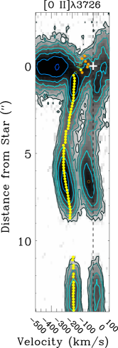
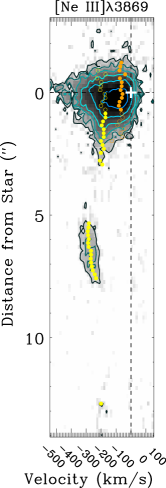
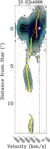
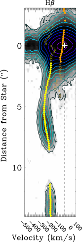
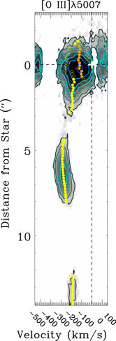
Figure 4: Selected PV diagrams of bright emission lines from the VLT/X-Shooter UVB spectra, showing [O ii] $\lambda 3726$, [Ne iii] $\lambda 3869$, [S ii] $\lambda 4068$, H$\beta$, and [O iii] $\lambda 5007$. The line profiles have been decomposed into high-velocity (yellow) and low-velocity (orange) components. At each position, the fitted velocity centroids of the components are overlaid on the PV diagrams, with the stronger component shown by filled circles and the weaker component by open circles. In all the PV diagrams, the contours start from $3\sigma$ ($1\sigma=3\times 10^{-18}$ erg s^-1 cm^-2 Å^-1) and increase by factors of 2.

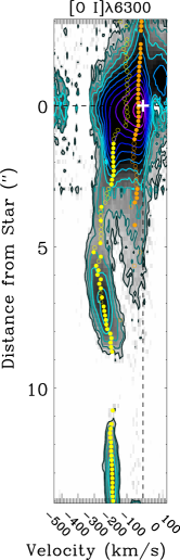
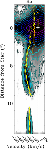
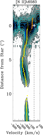
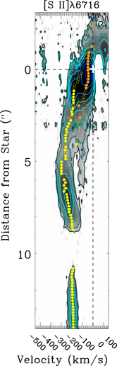
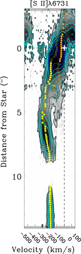
Figure 5: Selected PV diagrams of bright emission lines from the VLT/X-Shooter VIS spectra, showing [O i] $\lambda 6300$, H$\alpha$, [N ii] $\lambda 6583$, [S ii] $\lambda 6716$, and [S ii] $\lambda 6731$. The line profiles have been decomposed into high-velocity (yellow) and low-velocity (orange) components. At each position, the fitted velocity centroids of the components are overlaid on the PV diagrams, with the stronger component in filled circles and the weaker component in open circles. In all the PV diagrams, the contours start from $3\sigma$ ($1\sigma=3\times 10^{-18}$ erg s^-1 cm^-2 Å^-1) and increase by factors of 2.

The 2010 VLT/X-Shooter spectra provide a larger field of view along the blueshifted jet. This data set provides an examination of ejection history after the 1999 HST/STIS observation. The evolution of the microjet and the high-velocity bow-shaped knot can be seen in the VLT/X-Shooter spectra. In order to match the features between the two observations, we assume a mean proper motion of $\sim 0\farcs 28\,{\rm yr}^{-1}$ for the knots in the blueshifted jet (Rodríguez et al., 2012). During the 11 years between the taking of the HST/STIS and the VLT/X-Shooter spectra any cohesive features will have moved outward by $\sim 3\arcsec$. In the following discussions we apply this offset in attempting to align features seen in the spectra and images.

Figures 4 and 5 show the continuum-subtracted PV diagrams of bright optical lines of the jet up to $\sim 14\farcs 2$ from the star. Three distinct emission regions can be identified from the PV diagrams. (1) The strongest peak occurs within $\sim 0\farcs 5$ of the stellar position. The emission traces the flow with a trend of increasing speed and decreasing line intensity up to a local minimum at $\sim 4\arcsec$ from the star. This coincides with the region interior to knot k3 (Rodríguez et al., 2012) found in the [Fe ii] wind (Takami et al., 2002; Pyo et al., 2003) observed in 2001 to 2002, and may also correspond to the innermost $\lesssim 1\arcsec$ region of the 1999 STIS spectra (Maurri et al., 2014) and the [Fe ii] microjet observed in 2005 (Agra-Amboage et al., 2011; White et al., 2014). We identify the first emission peak and the extension as the “star $+$ microjet” region. (2) The second region peaks at $\sim 6\farcs 5$ and may be identified with the bow-shaped knot observed at $3\farcs 6$ in 1998 (Lavalley-Fouquet et al., 2000), denoted as knot B by Eislöffel & Mundt (1998). The knot A (or knot k2 in Rodríguez et al., 2012) identified at $0\farcs 93$ in 1998 (Lavalley-Fouquet et al., 2000) and $1\farcs 3$ in 1999 (Maurri et al., 2014) appears to have dissipated by 2009. It may have contributed to the velocity maximum observed at $\sim 5\farcs 5$. We denote this region as “knot A$+$B.” (3) The third region, peaked at $\sim 13\farcs 2$, is truncated by the edge of the detector. We identify this region as “knot C.”

Overall, the kinematic features of emission lines of the different species are similar, with slight differences in the shapes and widths of the lines. In the “star $+$ microjet” region, all species have broad line profiles that show either double emission peaks or a prominent peak blended with a weaker “shoulder.” We decomposed the lines as in Section 3.1, and have overplotted the fitted velocity centroids in Figures 4 and 5, with the HVC in yellow and the LVC in orange. For positions that require double-Gaussian fitting, velocity centroids of the stronger component are shown as filled circles and those of the weaker component are shown as open circles.

The LVC is confined to within $\sim 3\arcsec$ of the star and is less extended than the HVC. For all species, the LVC appears stronger than the HVC within the innermost $1\arcsec$. The HVC becomes dominant outside $1\arcsec$ and extends beyond $3\arcsec$. Some of the high-ionization and high-density lines, including [Ne iii] and [O iii], are undetected beyond $\sim 3\arcsec$ and reappear after $\sim 5\arcsec$. The HVC velocity centroids gradually increase from $-180$ km s^-1 at $1\arcsec$ to $-230$ km s^-1 at $3\arcsec$. The velocity maxima of $\sim-260$ km s^-1 are reached near the beginning of knot A at $\sim 5\arcsec$ and decrease steadily to $\sim-170$ km s^-1 at the end of knot B at $\sim 9\arcsec$. At knot C, the jet has a steady velocity of $\sim-200$ km s^-1. Table 2 summarizes the kinematic properties of several forbidden emission lines obtained from Gaussian decomposition of the 2010 VLT/X-Shooter spectra.

The X-Shooter spectra show that most of the permitted line profiles are centered at the position and systemic velocity of DG Tau. Permitted lines that may be related to accretion flow, such as H i, He i, and Ca ii, are broad, extending up to $\pm 450$ km s^-1. For some of the lines, such as H i Balmer series (H$\alpha$ to H$\zeta$), Ca ii H and K, and He i (specifically $\lambda 5876$ and $\lambda 7065$), profiles are asymmetric with an extension to the blue. These lines also show spatially resolved emission from knot A$+$B, where the kinematic structures are consistent with forbidden lines that trace the jet emission.

Table 2: Kinematic Properties from the 2010 VLT/X-Shooter Spectra

	[Ne iii] $\lambda 3869$	[S ii] $\lambda 4068$	[O iii] $\lambda 5007$	[O i] $\lambda 6300$	[N ii] $\lambda 6583$	[S ii] $\lambda 6731$
Component (Region)	median $\pm$ std dev. (km s-1)
LVC (microjet)	$-69.32\pm 23.6$	$-67.33\pm 7.46$	$-87.97\pm 17.9$	$-43.11\pm 10.5$	$-118.0\pm 48.0$	$-68.63\pm 23.9$
HVC (microjet)	$-187.5\pm 11.8$	$-187.7\pm 23.6$	$-189.6\pm 14.8$	$-182.7\pm 29.2$	$-187.0\pm 14.0$	$-184.3\pm 27.6$
HVC (A$+$B)	$-268.0\pm 24.5$	$-258.5\pm 25.4$	$-272.5\pm 15.8$	$-258.1\pm 34.9$	$-260.0\pm 35.0$	$-260.0\pm 31.9$
HVC (knot C)	$-187.5\pm 13.2$	$-188.2\pm 7.64$	$-186.0\pm 6.60$	$-192.1\pm 5.13$	$-193.0\pm 10.1$	$-190.5\pm 4.76$

3.3 Properties of the [Ne iii] $\lambda 3869$ Velocity Components

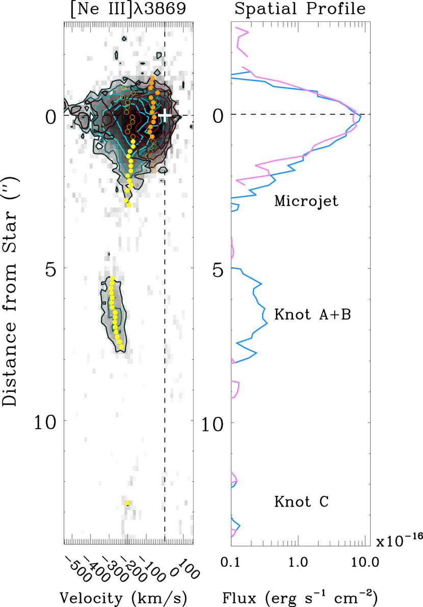
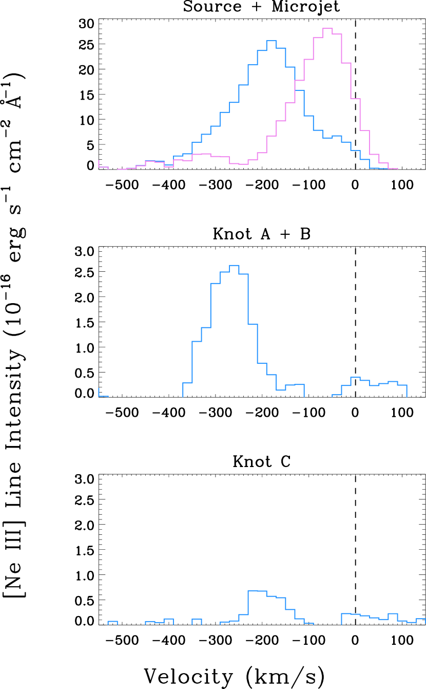
Figure 6: Kinematic properties of velocity-decomposed [Ne iii] $\lambda 3869$ emission are shown in a PV diagram (left panel), a spatial profile along the jet axis (central panel), and line profiles at specific spatial positions (right three panels). In the PV diagram, the decomposed HVC and LVC are shown by green and red contours, respectively. The yellow symbols represent the HVC velocity centroids and orange symbols represent the LVC velocity centroids; the filled symbols indicate the stronger component at each specific position whereas the open symbols indicate the weaker component, as in Figure 4. The spatial profile is shown on a logarithmic scale to accommodate the large contrast between the innermost 3″emission and the outer knots.

Figure 6 shows the kinematic properties of the velocity-decomposed [Ne iii] $\lambda 3869$ emission as PV diagrams, spatial profiles, and line profiles at specific spatial positions along the jet. [Ne iii] $\lambda 3869$ is detected toward the innermost 3″ (star $+$ microjet) and between 5″ and 8″ (knots A and B), and is marginally detected at knot C. The integrated fluxes for the three regions are $10.82\pm 0.09\times 10^{-15}$, $5.19\pm 0.26\times 10^{-16}$, and $1.25\pm 0.26\times 10^{-16}$ erg s^-1 cm^-2, respectively.

The decomposed [Ne iii] $\lambda 3869$ PV diagrams (Figure 7) show the velocity components in the innermost 3″ of the flow. After decomposition, the overall peak at $\sim-100$ km s^-1, $\sim 0\farcs 2$ from the star, breaks into two peaks of similar intensities at $\sim-180$ km s^-1 for the HVC and $\sim-70$ km s^-1 for the LVC. The HVC peak has a line width of $\sim 200$ km s^-1 at 0$\farcs$2, larger than the LVC line width of $\sim 120$ km s^-1 at the same position. The LVC has relatively stable line widths within to 1″, whereas the HVC shows decreasing line widths from the maximum value of $\sim 200$ km s^-1 to $\sim 100$ km s^-1 at $\sim 2\arcsec$. There is a non-Gaussian wing extending to $\sim-500$ km s^-1. The total fluxes in the HVC and LVC components within $\pm 3\arcsec$ are $5.3\pm 0.1\times 10^{-15}$ and $4.8\pm 0.1\times 10^{-15}$ erg s^-1 cm^-2, respectively. The kinematic properties of the decomposed [Ne iii] $\lambda 3869$ emission along the regions in the jet are summarized in Table 3.

Table 3: Properties of the [Ne iii] $\lambda 3869$ Jet of DG Tau

		Velocity Centroid	Velocity Width	Flux
		km s-1	km s-1	erg s-1 cm-2
Microjet	LVC	$-69.32\pm 23.6$	$107.4\pm 28.6$	$4.8\pm 0.1\times 10^{-15}$
	HVC	$-187.5\pm 11.8$	$123.0\pm 38.0$	$5.3\pm 0.1\times 10^{-15}$
Knot A$+$B		$-268.0\pm 24.5$	$103.6\pm 14.1$	$5.2\pm 0.3\times 10^{-16}$
Knot C (part)		$-187.5\pm 13.2$	$100.7\pm 88.8$	$1.3\pm 0.3\times 10^{-16}$

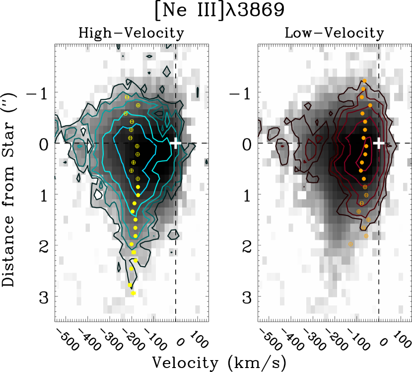
Figure 7: Velocity-decomposed PV diagrams of [Ne iii] $\lambda 3869$ from the innermost 3″ blueshifted microjet. The left and right panels show the HVC and LVC PV diagrams, respectively. Both contours start from $3\sigma$ ($\sigma=3.0\times 10^{-18}$ erg s^-1 cm^-2) and increase by factors of 2. The background grayscale maps are the original PV diagrams without velocity decompositions. The Gaussian-fitted velocity centroids are overlaid. The filled symbols indicate the stronger component at that spatial position and the open symbols indicate the weaker component.

4 On the Possible Origins of [Ne iii] Emission in the DG Tau Jet

4.1 [Ne iii] Microjets from Low-Mass Young Stars

DG Tau is one of the few low-mass YSOs known to show bright [Ne iii] $\lambda 3869$Å emission in the arcsecond-scale microjet. The [Ne iii] emission shares kinematic properties with other forbidden emission lines tracing the jet (e.g., [O i], [S ii], and [N ii]), notably the two velocity components at $-180$ and $-70$ km s^-1. However, because of its higher ionization potential and higher critical density, the emission is restricted to the innermost 3″ microjet and the 7″ knot.

The presence of [Ne ii] and [Ne iii] emission from the jet may require that high-energy photons be present either at the launching site or during the propagation of the jet. Doubly ionized neon arises from either ionization of valence electrons, which requires a total energy of 62.5 eV, or the photoionization of K-shell electrons, which requires a photon energy $>$0.903 keV. In the low-mass circumstellar environment, valence electrons may be ionized by extreme ultraviolet (EUV) photons or by collisions in shocks with shock speeds higher than 100 km s^-1 (Hartigan et al., 1987; Hollenbach & Gorti, 2009). K-shell photoionization must occur close to the star (Glassgold et al., 2007), a copious source of keV X-rays.

As described in Section 1, the X-ray source DG Tau is bright, spatially extended, and consists of at least three distinct components. The strongest component, located at the nominal stellar position, is likely thermal emission from hot ($\sim$20–30 MK) coronal gas confined in magnetic loops (Güdel et al., 2008). The soft extended X-ray emission is concentrated $\sim 5\farcs 5$ from the star. Its proper motion of 0$\farcs$28 yr^-1 suggests association with non-standing shocks in the jet (Güdel et al., 2012; Rodríguez et al., 2012). The third component, the soft source 0$\farcs$2 from the star, exhibited no significant proper motion over a 2 yr period from 2004 to 2006 (Schneider & Schmitt, 2008). The emission could be produced by $\sim 450$ km s^-1 shocks in the innermost dense jet (Günther et al., 2009), colliding stellar and magnetocentrifugal winds (from the inner disk; Günther et al., 2014), or reconnections of magnetic fields threading the jet (Schneider et al., 2013b).

The first known [Ne iii] microjets from low-mass YSOs were discovered toward Sz 102 (Liu et al., 2014). The nearly edge-on orientation of the Sz 102 system presents a different geometry for comparison with the jet of DG Tau. In Sz 102 the [Ne iii] $\lambda 3869$ emission appears unresolved within $\sim 200$ au in the ground-based VLT/Uves spectra and shows a broad line profile with “excess” emission across the systemic velocity. This suggests that the jet originates from a wide-angle wind close to the star. The neon may be ionized by large hard X-ray flares generated by reconnection events from field lines twisted by star–disk interactions within the regions encompassed by the wide-angle wind and may then be carried out through the wind flow. Further monitoring of the system would be required to test the postulation since virtually nothing is known about hard X-ray flares or temporal variability of the [Ne iii] line in Sz 102.

For DG Tau, we discuss the origins of its [Ne iii] jet in the following subsections. In summary, we suggest that the neon ionization in the innermost microjet may be largely attributed to the photoionization by a series of flares from a bright hard X-ray source and the slow recombination of the innermost hot jet heated through either jet shocks, recollimated stellar wind shocks, or magnetic reconnection. A contribution from shock ionization in the jet is still possible, though the fraction of shock dissipation must be small in order to be consistent with the inferred soft X-ray luminosity. The detection of the outer [Ne iii] knot would favor strong shock ionization in the jet, which may also account for the soft X-ray extension along the jet axis.

4.2 Ionization of the Inner 3″ Microjet: Shocks and Soft X-rays?

Shocks can be an efficient ionization source for neon when the postshock temperature reaches the order of megakelvin, above which collisional ionization is important. At several megakelvin, thermal gas emits mainly in soft X-rays which peak at $<1$ keV. To reproduce the spectral energy distribution of the 0$\farcs$2 soft X-ray component at $\sim 2$ MK requires a shock speed $v_{\rm s}\approx 480$ km s^-1, gas temperature of $\sim 0.3$ keV, and volume emission measure of $\sim 10^{52}$ cm^-3 (Günther et al., 2009). To satisfy these constraints, the cooling length and cross section of the modeled shock must both be of the order of au, with the mass flux through the shock of the order of $10^{-11}$ – $10^{-10}$ $M_{\odot}$ yr^-1 (Günther et al., 2009). The ratio between the mass flux in the shock and the total mass-loss rate of DG Tau ($\sim 10^{-7}$ $M_{\odot}$ yr^-1), $\sim 10^{-4}$ – $10^{-3}$, may be regarded as the fraction of shock dissipation $f_{\rm sh}$ as in Hollenbach & Gorti (2009). One can compare the theoretical and observed [Ne ii] 12.81µm flux using Equation (33) of Hollenbach & Gorti (2009). Putting $n_{0}\approx 10^{5}$ cm^-3, $v_{\rm s}\approx 480$ km s^-1, and $f_{\rm sh}\approx 10^{-3}$, the predicted luminosity is $10^{-6}L_{\odot}$, two orders of magnitude fainter than the observed Spitzer value ($\sim 2\times 10^{-4}L_{\odot}$, Güdel et al., 2010). Although the Spitzer observation is spatially unresolved, the expected contribution from the disk atmosphere would be at the level of $\sim 10\%$ (Güdel et al., 2010). The bulk of the [Ne ii] 12.81µm flux must arise via a different mechanism.

Pure shock models, whether planar shocks or bow shocks, make predictions of line ratios (e.g., Hartigan et al., 1987) that can be compared with our data. The main adjustable parameters are the shock velocities and preshock densities. High-ionization forbidden lines, such as [Ne iii] $\lambda 3869$ and [O iii] $\lambda 5007$, and UV permitted lines, such as C iv $\lambda 1550$, appear only when shock velocities exceed $\sim 100$ km s^-1. For forbidden emission lines, the relative intensities increase as shock velocity increases, until collisional de-excitation becomes important at velocities higher than $\sim 300$ km s^-1. For example, as shock velocities increase from 100 to 300 km s^-1, [O iii]/H$\beta$ decreases from $\sim 4.0$ to $\sim 2.5$, and [Ne ii] 12.81µm/H$\beta$ decreases from $\sim 3.0$ to $\sim 1.5$. The relative flux of UV permitted lines decreases as the Balmer intensity increases since more ionizing photons in the shock front are absorbed by H atoms: C iv/H$\beta$, for example, decreases from $\sim 20.0$ to $\sim 5.5$. The [Ne iii]/H$\beta$ ratio, on the other hand, increases by $\sim 20$% as shock velocity increases from 300 km s^-1, and approaches $\sim 1.0$. This results in decreasing line ratios of C iv/[Ne iii], [O iii]/[Ne iii], and [Ne ii]/[Ne iii] for shock speeds exceeding 300 km s^-1. The C iv/[Ne iii] ratio approaches $\sim 10$, the [O iii]/[Ne iii] ratio approaches 3, and [Ne ii]/[Ne iii] approaches 1 for high-velocity shocks. The observed ratios for the inner 3″ jet in the HVC are (dereddened with $A_{V}\approx 0.55$ as in Schneider et al., 2013a) [Ne iii]/H$\beta$ $\sim 0.15$, [O iii]/H$\beta$ $\sim 0.12$, and C iv/H$\beta$ $\sim 1$, which give C iv/[Ne iii] $\sim 8$, [O iii]/[Ne iii] $<1$, and [Ne ii]/[Ne iii] $\sim 24$. The C iv/[Ne iii] ratio appears to be similar to the ratio in the shocked gas but the [O iii]/[Ne iii] and [Ne ii]/[Ne iii] ratios are not consistently reproduced. The high [Ne ii]/[Ne iii] value, as produced by high [Ne ii]/H$\beta$ and low [Ne iii]/H$\beta$, occurs more readily in the mild shock condition when the shock speed is lower than $\sim 100$ km s^-1. However, this would be inconsistent with the assumption that the soft X-rays are produced by strong shocks in the jet. Discrepancies from the crude comparison of line ratios can be due to the different spatial coverages of the line species that cannot to be resolved from spatially summed spectra. Spatially resolved spectra and a shock model detailing the geometry are needed to account for possible spatial variations of the flux ratios.

An alternative explanation for the 0$\farcs$2 stationary X-ray source is the collimation shock where the tenuous stellar wind collides with the inner boundaries of the magnetocentrifugal winds emerging from the inner region of the circumstellar disk (Günther et al., 2014). A soft X-ray source produced by this stationary shock lies outside the jet and can irradiate it. The X-ray ionization rate of doubly ionized neon depends on the X-ray luminosity and the branching ratio of the production rate from neutral to doubly ionized neon. These soft X-rays are an order of magnitude fainter than the harder coronal X-rays (Güdel et al., 2008). The branching ratio required for the soft X-ray to doubly ionize neon is $\sim 0.1$, much smaller than $\sim 0.94$, that for the hard X-ray (Glassgold et al., 2007). Therefore, even if the soft X-ray irradiation contributes to neon ionization, in this scenario the expected ionization rate will be more than an order magnitude smaller than that provided through harder coronal X-ray irradiation.

4.3 Ionization of the Inner 3″ Microjet: Hard X-Rays and Flares?

The keV photons from the harder coronal X-ray source coincident with the star (Güdel et al., 2008; Schneider & Schmitt, 2008) provide a more efficient source for ionizing the neon. The large ionization flux from hard X-rays can produce a large fraction of electrons. The large wind mass-loss rate of DG Tau ($\dot{M}_{\rm w}\sim 10^{-7}$ $M_{\odot}$ yr^-1) produces relatively dense regions in the jet. Combining the two effects, sufficient collisional excitation can be maintained to explain the observed [Ne iii] $\lambda 3869$ flux. By reproducing the observed mid-infrared [Ne ii] and [Ne iii] luminosities of jet-driving low-mass YSOs, Shang et al. (2010) demonstrated that both X-ray ionization and high mass-loss rate are crucial to sustain a high collisional excitation rate. In contrast to the strong shock scenario, photoionization by keV photons is the main ionization source (Glassgold et al., 2007). Only mild shocks with speeds $\lesssim 50$ km s^-1 are needed in the jet to maintain the temperature and ionization fraction for the formation of optical forbidden emission lines. The observed [Ne iii] $\lambda 3869$ HVC flux, dereddened using $A_{V}=0.55$, corresponds to a luminosity of $\sim 2.7\times 10^{28}$ erg s^-1. The model of Shang et al. (2010) would require an averaged X-ray luminosity $L_{\rm X}\lesssim 10^{31}$ erg s^-1, or about an order of magnitude larger than observed, to explain the [Ne iii] luminosity, for the inferred $\dot{M}_{\rm w}$. The apparent discrepancy can be accounted for by the fact that the X-ray luminosity adopted in the model refers to the intrinsic, averaged value of X-ray luminosity. The intrinsic X-rays for T Tauri stars with mass accretion rate higher than $10^{-8}\,M_{\odot}\,{\rm yr}^{-1}$ are inferred to be deficient by more than an order of magnitude (Telleschi et al., 2007; Bustamante et al., 2016). The averaged value may also be elevated when flares are taken into account.

Stellar flares could produce the required ionizing flux for the observed neon ionization and [Ne iii] $\lambda 3869$ intensity. X-ray surveys of low-mass young stars in star clusters and associations show that impulsive flares typically occur on a timescale of weeks and rise to average luminosities of $\sim 6\times 10^{30}$ erg s^-1 in a day or two (Wolk et al., 2005). Larger but rarer flares of $\sim 100$ MK with luminosities up to $\sim 10^{32}$ erg s^-1 have been observed (Imanishi et al., 2001; Grosso et al., 2004; Favata et al., 2005; Getman et al., 2008a, b). These strong flares may be associated with reconnections in closed loops of stellar magnetic fields extending to several stellar radii (Favata et al., 2005). Interactions between the star and its circumstellar disk can also induce reconnections and flares (Shu et al., 1997).

The flare frequency of DG Tau is poorly known. DG Tau has been observed by Chandra in several short exposures (each $\sim 30$ ks) in 2004–2006, and three long exposures (each $\sim 120$ ks) in 2010 January (Güdel et al., 2012). The long exposures captured two flare events within three days with durations of 30 and 50 ks, respectively. The strongest flare on 2010 January 5, just two weeks before our VLT/X-Shooter observation, shows an increase of five times the average luminosity of the X-ray emission at energies above 1 keV. Such a large X-ray luminosity, $\sim 5\times 10^{30}$ erg s^-1, may contribute a significant fraction of the neon ionization. At densities below the critical density of [Ne iii], frequent X-ray flares could maintain the observed emission measure. Since we do not have a good record of the [Ne iii] flux, further extrapolations and predictions are dangerous.

If neon is ionized primarily by hard X-ray flares, the [Ne iii] emission will peak close to the ionization source, where the ionization rate and collisional excitation rate are the maximum. The line intensity will gradually decrease as the flow propagates due to recombination of the doubly ionized neon. The observed [Ne iii] $\lambda 3869$ spatial profile along the jet axis is basically consistent with this scenario of ionization and recombination (Figure 6).

In this scenario, how far the doubly ionized neon can extend along the jet depends on how long the ionization remains frozen-in along the flow if no strong secondary ionization source occurs during propagation of the jet. The observed spatial extent of the emission may be compared against the expected extent that is determined by the estimated values of the recombination timescale and the flow timescale. The high-velocity [Ne iii] microjet originates close to the source and extends up to 2″–3″. This is among the shortest extent of any of the observed forbidden HVC emission from the DG Tau microjet. The radial velocity of the HVC is $\sim-180$ km s^-1. If a line-of-sight inclination of $\sim 40\arcdeg$ is assumed (Eislöffel & Mundt, 1998; Schneider et al., 2013a), the derived proper motion on the plane of sky is 0$\farcs$23 yr^-1 at the distance of 140 pc. If no further ionization occurs in the flow, the neon gas would require a recombination timescale of $\sim 10$ yr in order to explain the extended emission. The recombination timescale of [Ne iii], $t_{\rm rec}$ , scales as $(n_{e}\alpha(T))^{-1}$. Using the coefficient $\alpha(T)\approx 1.7\times 10^{-12}(T/10^{4}\,{\rm K})^{-2/3}$ (Glassgold et al., 2007; Shang et al., 2010), the recombination timescale is of the order of $\sim 1$ yr if $T\lesssim 3\times 10^{4}$ K and $n_{e}\approx 3\times 10^{4}$ cm^-3 as implied by the red [S ii] doublet and [O i]/[N ii] (e.g., Coffey et al., 2008; Maurri et al., 2014). Other sources to maintain the ionization or temperature may be needed to increase the recombination timescale in order to better interpret the observation.

The soft X-ray source at $\lesssim 0\farcs 2$ from the star (Güdel et al., 2008; Schneider & Schmitt, 2008) may alternatively help to maintain the frozen-in ionization of the flow by contributing to jet heating. The hot ($T\gtrsim 10^{5}$ K) C iv jet, detected in 2011 somewhat downstream from the soft X-ray source, was considered to be a consequence of the heating (Schneider et al., 2013a, b). The peak emission is at $\sim-180$ km s^-1, consistent with the velocity of HVC [Ne iii] emission obtained $\sim 1$ yr earlier. The association of the C iv jet with the [Ne iii] HVC suggests that the lower-temperature emission of the jet may be a continuation of the hot jet. This hot portion of the jet can help drag out the recombination timescale to $\sim 10$ yr and may account for the extended emission of the [Ne iii] line. In this scenario, the jet is propagating through the apparently stationary local heating region. The heating can be due either to a jet shock of speed $\sim 450$ km s^-1 (Günther et al., 2009) or to a recollimation shock of a stellar wind with velocity of $\sim 840$ km s^-1 obliquely hitting a magnetocentrifugal wind (Günther et al., 2014). The heating may also produce soft X-ray photons that partially contribute to C iv and [Ne iii] emission. Heating may also come from magnetic recombination of the field lines threading the jet (Schneider et al., 2013a). Specifically, the magnetic recombination in the jet fields may produce keV photons and provide additional ionization of neon gas in the jet.

For the ionization of the inner microjet, both the mechanisms of strong shocks and hard X-rays have their respective applicabilities and challenges. Shock ionization can account for the neon ionization and the soft X-ray emission 0$\farcs$2 from the star if the shock speed reaches $\sim 480$ km s^-1. However, the fraction of shock dissipation that matches the X-ray luminosity may be two orders of magnitude lower than that needed to sustain the observed flux of [Ne ii] and [Ne iii] and does not match the [Ne ii]/[Ne iii] ratio predicted in shock models. The hard coronal X-rays from the close vicinity of the star can overcome the threshold energy for neon photoionization, but an elevated average hard X-ray luminosity greater than the observed value would be required to penetrate the outflowing gas for the inferred mass-loss rate. The observed flares from DG Tau can provide the elevated luminosity to fulfill this requirement. We further postulate the source of the flares that can match the requirement in Section 5.

4.4 Ionization of the 6$\farcs$5 Knot: Shocks in the Jet?

The [Ne iii] HVC is absent between 3″ and 5$\farcs$5, which is where knot A$+$B appears. The spatial discontinuity suggests that the physical conditions in the jet become less favorable for formation of the neon line such that the flow timescale cannot compete with the recombination timescale at distances larger than $\sim 3\arcsec$. At the outer knot, either the neon gas is reionized to a doubly ionized state or the electron density increases such that the excitation conditions favor [Ne iii] emission, or both. From the PV diagram, the [Ne iii] emission decelerates from $\sim-290$ km s^-1 at 5$\farcs$5 to $\sim-210$ km s^-1 at 8″. When compared with the arcsecond-resolution HST/STIS long-slit spectra, this region corresponds to the knots B0 and B1 that also show a clear velocity jump from $\sim-290$ km s^-1 to $\sim-210$ km s^-1 (Maurri et al., 2014). Taking into account for the inclination angle, the velocity jump is $\sim 100$ km s^-1, which may be sufficient for in situ neon ionization if the velocity jump is interpreted as a strong shock in the jet flow (Hollenbach & Gorti, 2009).

The shocks responsible for the neon ionization in the outer knot may also result in the extended X-ray emission of DG Tau. Adjacent to the [Ne iii] knot at $\sim 6\farcs 5$, the X-ray knot is at $\sim 5\farcs 5$ in the 2010 Chandra image. It was discovered at 4$\farcs$3 in 2005, and thus shows a proper motion of $\sim 0\farcs 27$ yr^-1 similar to those of other optical and infrared knots (Güdel et al., 2008, 2012; Rodríguez et al., 2012). Tracing this proper motion back in time, the X-ray knot would have appeared in the $\sim 2\farcs 4$ interknot region between knots A1 and B0 in the 1999 HST/STIS spectra (Maurri et al., 2014) and the 1998 CFHT/OASIS spectra (Lavalley-Fouquet et al., 2000). Comparisons of the PV diagrams between the 1999 STIS spectra and the 2010 X-Shooter spectra show that the maxima of the velocity centroids have decreased from $\sim-360$ km s^-1 to $\sim-290$ km s^-1, which also coincides with the velocity jump between A1 and B0 (Maurri et al., 2014). The interknot region may produce adequate ionization from shocks but the higher densities downstream are more favorable for line production. The velocity difference of $\sim 100$ km s^-1 would be deprojected to $\sim 130$ km s^-1 for an inclination $i\approx 38\arcdeg$. The observed velocity jump appears to be less than the required $\sim 380$ km s^-1 (Draine & McKee, 1993) if shock is the main heating source for the 2.7 MK X-ray knot. A magnetic field carried by the flow may be working to reduce the shock strength and provide additional heating (Güdel et al., 2008), although the field structures in the flow need further observations and modeling to be confirmed.

5 Temporal Variations in the HVC of the DG Tau Jet

5.1 The Double Velocity Components of DG Tau

DG Tau is known to have distinct double-peaked velocity profiles in its jet emission (Hartigan et al., 1995). Solf & Böhm (1993) used long-slit spectra to show the different properties of the two components: a compact LVC at $-50$ km s^-1 appears close to the source, and a HVC at $-260$ km s^-1 is offset from the source by $\sim 0\farcs 2$ and extends beyond 2″ with a lower velocity of $\sim-200$ km s^-1. Among the line species detected in the spectra, [O i] $\lambda 6300$ appears in both components, [N ii] $\lambda 6583$ is dominant in the HVC, and [S ii] $\lambda 6731$ is dominant in the LVC. From the 1999 HST/STIS spectra, we again show that both velocity components exist in the first 0$\farcs$7 of the microjet and that different line species dominate in different velocity components. In the near infrared, DG Tau also possesses [Fe ii] 1.644µm emission that can be decomposed into a more compact and transversely broader LVC, and a more extended and transversely narrow HVC (Pyo et al., 2003; Agra-Amboage et al., 2011; White et al., 2014). The [Fe ii] HVC is typically $\sim-200$ km s^-1, and the LVC is $\sim-100$ km s^-1. The velocity centroids of the [Fe ii] LVC are similar to those of [N ii] and faster than those of [O i] and [S ii]. Yet another molecular wind component, detected through H₂, appears as a wide-angle, low-velocity ($\sim-15$ km s^-1) emission close to the source (Agra-Amboage et al., 2014; White et al., 2014). The two-component profiles in the atomic lines, observed through spatially resolved spectra taken from 1980 to 2010, appear to have persisted for several decades in the DG Tau jet.

That the different line species are dominant in different velocity components is often considered to be consistent with an “onion-shaped” outflow structure (Bacciotti et al., 2000; Pyo et al., 2003). In this scenario, the density and velocity structures, as well as excitation conditions, are layered across the jet axis. The species with higher excitation criteria (e.g., [N ii]) appear in the central region in which the velocity and density are higher, whereas those with lower excitation conditions and lower critical densities (e.g., [S ii]) appear in the outer region with lower velocities. On the other hand, this can also be achieved by a cylindrically stratified wide-angle wind, similar to a steady-state X-wind. As described in Shang et al. (2006, 2010), the divergent streamlines contribute to the large line widths of the HVC, and axially concentrated density provides the bulk line emission and narrow appearance of the HVC, whereas the ambient material may be mildly shocked to produce the LVC and the even slower molecular layer. For young flat-spectrum stars, the remaining envelope can provide the remnant ambient material. In the cases of DG Tau (Testi et al., 2002) and HL Tau (Cabrit et al., 1996), a remnant envelope perpendicular to the outflow has been detected, and low-velocity wide-angle H₂ emission encompassing the star and the [Fe ii] jet is found (Takami et al., 2007; Agra-Amboage et al., 2014; White et al., 2014). Regardless of the interpretations, the emission of the HVC and LVC should be decomposed and separated because of their differences in the line forming regions.

Through the analysis of two-Gaussian spectral decomposition, we show that the HVCs of [O i], [S ii], and [N ii] emission lines can have systematic differences in their respective velocity centroids. From the inner 0$\farcs$7 microjet in the 1999 STIS spectra, [N ii] shows a faster bulk radial velocity than [O i] and [S ii]. From the inner 3″ microjet in the 2010 X-Shooter spectra, different species have similar velocities. Explaining the different HVC centroids among species can be challenging for currently available models based on magnetocentrifugal wind. A steady-state X-wind can successfully describe a predominantly single HVC that is uniform among species, such as in RW Aur A (Liu & Shang, 2012) and in the 2010 X-Shooter spectra of DG Tau, but would require more complex ionization and heating profiles for the jet in order to explain the differences shown in the 1999 STIS spectra of DG Tau. The disk-wind model, with a layered velocity structure, also cannot fully address this issue (see, e.g., the similarity of the synthetic [O i] and [S ii] spectra in Rubini et al., 2014). In either interpretation, the [N ii] line emission traces the innermost dense region close to the jet axis and the velocity centroid represents the flow emanating from the innermost part of the disk. We regard velocity centroids traced by the [N ii] emission as the representative speed of the DG Tau jet in the subsequent discussions on temporal variations of the velocity components.

5.2 Temporal Variations of the Double Velocity Components

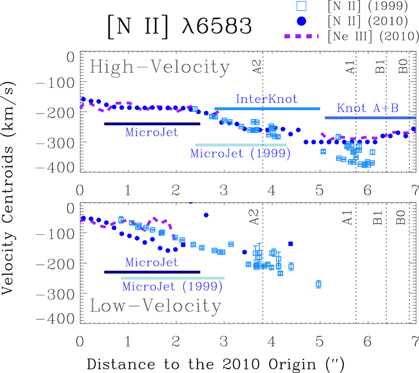
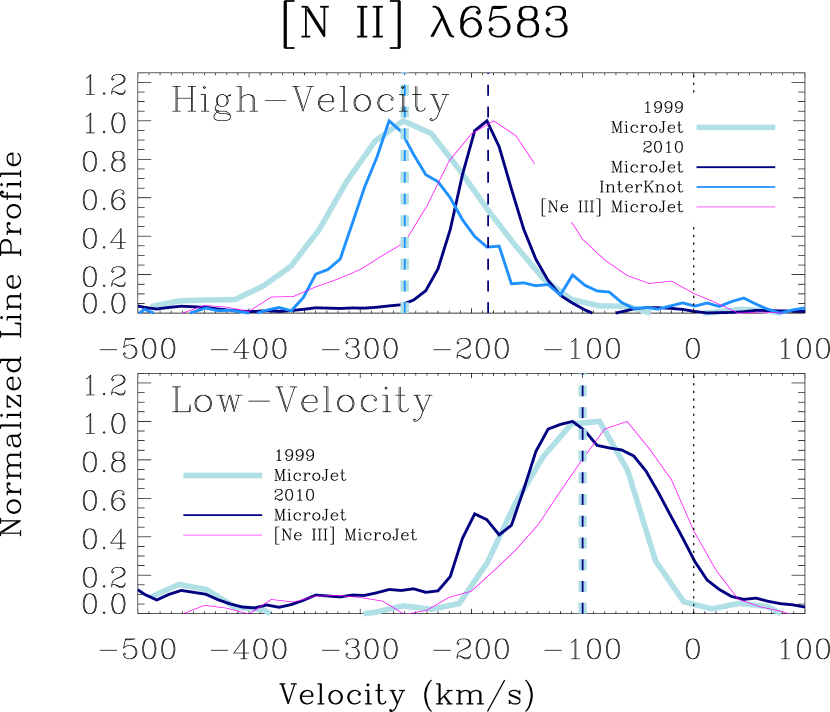
Figure 8: Variations of the [N ii] $\lambda 6583$ HVC and LVC centroids between the 1999 HST/STIS and 2010 VLT/X-Shooter spectra. The left panels compare spatial variations of the velocity centroids along the jet axis at the two epochs. The origin is set at the 2010 observational epoch, and the 1999 data are shifted to positions according to their respective velocity centroids, adopting the inclination angle ($\sim 38\arcdeg$, Eislöffel & Mundt, 1998) and distance (140 pc, Torres et al., 2007). The vertical dashed lines indicate the positions of features defined in Maurri et al. (2014), shifted according to their respective velocity centroids obtained from the 1999 spectra. The 1999 (open squares) and 2010 (filled circles) [N ii] data are compared against [Ne iii] $\lambda 3869$ (thick dashed lines) from the 2010 data. The regions of “MicroJet,” “InterKnot,” and “Knot A$+$B” are defined based on the [Ne iii] features, and the “MicroJet (1999)” region is defined by the positions of the shifted 1999 velocity centroids. The right panels compare the line profiles at the two epochs, normalized to their individual maxima. The light thick lines are the velocity-decomposed profiles of [N ii] from the 1999 data, obtained by summing the spectra over the “MicroJet (1999)” region. The strong thin lines are those from the 2010 data; the darker profiles sum over the “MicroJet” region and the lighter profiles sum over the “InterKnot” region. [Ne iii] $\lambda 3869$ profiles summed over the “MicroJet” region are shown for reference by thin purple lines.

While they are persistent, both velocity components of the DG Tau jet have varied. The most obvious differences can be seen by comparing the 1999 HST/STIS spectra and the 2010 VLT/X-Shooter spectra. As described above, the HVC centroids identified in the 1999 STIS spectra differ among species (cf. Figure 2), ranging from $\sim-150$ to $\sim-260$ km s^-1. Such differences seem to occur only in the innermost 0$\farcs$7 region in the 1999 STIS spectra. On the other hand, previous ejecta that correspond to the region of knots B0 and B1 show more uniform velocity centroids among [O i], [S ii], and [N ii] (Lavalley-Fouquet et al., 2000; Maurri et al., 2014). Post-1999 ejecta, e.g., those corresponding to the inner 3″ region in the 2010 X-Shooter spectra, also show uniform velocity centroids among species, with a median value of $\sim-180$ km s^-1. Understanding how the star transitions between these two phases and whether the phase with non-uniform velocity centroids will recur may require spectroscopic monitoring of the DG Tau jet. Variations in the LVC are less obvious. Within the innermost 1″, the velocities at the two epochs appear consistent.

The comparisons between the 1999 HST/STIS spectra and the 2010 VLT/X-Shooter spectra can be compared by matching their spatial and spectral resolutions. The spectral resolution for both observations is $\sim 65$ km s^-1. The main differences are the spatial resolution and the settings of the slit observations. The point spread function (PSF) of the HST optical instruments is defraction-limited to $\sim 0\farcs 1$, whereas that of the VLT is seeing-limited to $\sim 1\arcsec$ at the time of the observation. The slit widths match the PSF at observations, and the widths of 0$\farcs$1 and 1$\farcs$2 were used for STIS and X-Shooter, respectively. Although spatial resolutions cannot be matched, spatial coverages of the two observations can be kept similar for the analysis. Therefore, the STIS spectra transversely averaged across 0$\farcs$52 were used when comparisons of velocity centroids were made and longitudally averaged line profiles from both spectra were used to compare the overall representative spectral features between the two observational epochs.

Figure 8 compares the properties of the optical forbidden lines of the HVC and LVC between epochs 1999 and 2010, based on [N ii] $\lambda 6583$ emission from the two epochs. The left panels compare spatial variations of their velocity centroids. The positions of the 1999 data points have been shifted to the 2010 epoch to account for their proper motions according to their respective velocity centroids. The velocity centroids of [Ne iii] $\lambda 3869$ were overlaid to indicate the regions based on the features of [Ne iii] emission: the brightest “MicroJet” from 0$\farcs$5 to 2$\farcs$5, non-detected “InterKnot” from 2$\farcs$8 to 5$\farcs$0, and “Knot A$+$B” from 5″ to 8″. In the right panels, we compare the integrated [N ii] line profiles of the microjet between 1999 and 2010. The 1999 line profile is obtained by summing over 0$\farcs$1 to 0$\farcs$7 from the 1999 spectra, corresponding to the innermost microjet. The 2010 line profiles are obtained in two parts, one summing over the “MicroJet” region as the initial microjet in 2010, and another summing over the “InterKnot” region. For the HVC, the portion of the microjet in the 1999 data matches the 2010 “InterKnot” region well in both velocity centroids and positions. This suggests that the initial microjet moves out without much interaction with previous ejecta in this region. For the LVC, the emission is not spatially extended and no clear interknot emission can be detected. The propagation or variation pattern is relatively unclear and does not show clear trends between the two epochs.

From comparisons of the spatial variations of velocity centroids, we conclude that the emission from the innermost microjet is not stationary. The HVC centroids of [N ii] $\lambda 6583$ have changed from a median value of $\sim-260$ km s^-1 in 1999 to $\sim-180$ km s^-1 in the 2010 X-Shooter spectra. The shifted 1999 data points for the microjet match those for the interknot region well in the 2010 X-Shooter data in both velocities and positions. The transitions appear to be smooth, and the matches in kinematic properties of between the two epochs suggest that the flow does not slow down significantly due to interactions with previous ejecta. The properties of both [N ii] and [Ne iii] emission lines in the microjet are consistent with a recombination flow. The [Ne iii] $\lambda 3869$ spatial profile is consistent with the flow recombining, and then being reionized, before the knot A$+$B. The average [S ii] $\lambda\lambda 6716/6731$ ratio increases from 0.5 to 0.8, corresponding to a decrease in $n_{e}$ from $\sim 10^{4}$ to $10^{2}$ cm^-3, at distances from 0$\farcs$5 to 4$\farcs$5, where the knot A$+$B starts to form with an increase in $n_{e}$ to $\sim 4000$ cm^-3. In the next subsection, we suggest a possible mechanism that might cause the decrease in the HVC velocity in the microjet and momentarily account for the dominant initial ionization in the microjet.

5.3 Possible Origin of the HVC Variation – Source of Flares in the System?

Comparison of the line profiles at two different epochs shows an overall decrease in jet speed from 1999 to 2010, without evidence for deceleration by discrete shocks. One possible cause of such a decrease in jet speed is the increase in the launching radius of the jet. Assuming that the terminal speed of the jet is proportional to the Keplerian speed at the launching radius and that the proportion remains the same for the two configurations at different epochs, the ratio of the two velocities ($180/260\approx 0.69$) corresponds to a change in the launching radius by a factor of $\sim 2$ ($(260/180)^{2}\approx 2.1$). At the inclination angle to the DG Tau system, the deprojected flow velocity in 1999 is $\sim 330$ km s^-1. As demonstrated in the X-wind sample fits to the jet and counterjet of RW Aur A in Liu & Shang (2012), the ratio of the terminal wind speed $v_{\rm w}$ to the Keplerian speed at the truncation radius, $v_{\rm x}$, can range from 1.5 to 3.5, depending on the mass loading in the magnetic field lines of the wind. If $v_{\rm w}/v_{\rm x}\sim 3$ is adopted, $v_{\rm x}\approx 110$ km s^-1. The estimated stellar mass of DG Tau is $0.7\pm 0.2M_{\odot}$ (see Hartigan et al., 1995; Testi et al., 2002), and one may derive the truncation radius $R_{\rm x}=GM_{\ast}/v_{\rm x}^{2}\approx 0.05\pm 0.02$ au. In this scenario, the change in HVC centroids may correspond to a change in truncation radius from 0.05 au in 1999 to 0.10 au in 2010.

One possible explanation for the increase in the disk truncation radius is an expansion of the stellar magnetosphere, which pushes out the disk. At equilibrium, the inner edge of the disk can corrotate with the star due to regulation by the magnetic field connecting the star and the disk. When the magnetosphere expands, the inner edge of the disk will change from one equilibrium to a new equilibrium position further away from the star with a lower Keplerian speed. During the transition, the angular speed of the star and the inner disk edge may not coincide with each other, i.e., $\Omega_{\ast}\neq\Omega_{\rm x}$. This may induce magnetic reconnections for the field lines connecting the star to the disk, and a fraction of the energy release may contribute to the hardening of X-rays. In the fluctuating X-wind theory (Shu et al., 1997), the amount of X-ray luminosity generated through magnetic reconnection is proportional to the square of the (dimensionless) dipole flux $\Phi_{\rm dx}$ of order unity and the energy scale for disk accretion, $\frac{GM_{\ast}\dot{M}_{\rm D}}{R_{\rm x}}$, both computed at the truncation radius. This proportional factor, which may range from 0.1 to 0.01, depends on the fraction of magnetic energy released, aside from that used for particle acceleration, and on the efficiency of energy conversion. Taking the disk accretion rate $\dot{M}_{\rm D}$ to be of the same order as the mass accretion rate onto the star $\dot{M}_{\rm acc}$, the energy scale for disk accretion is of the order of $\sim 10^{33}$ erg s^-1. The resulting total X-ray luminosity would be of the order of $\sim 10^{31}$ to $\sim 10^{32}$ erg s^-1 and is sufficient to power the hard X-ray source close to DG Tau and to account for the ionization for [Ne iii] $\lambda 3869$ emission in the jet.

6 SUMMARY

We have studied the kinematics and ionization properties of the DG Tau jet using archival HST/STIS spectra taken in 1999 January and new VLT/X-Shooter spectra taken 11 years later. For both data sets, we identify an HVC that is spatially extended and connected to outer knots and an LVC that dominates within $\pm 1\arcsec$ through Gaussian decomposition. Optical [O i], [S ii], and [N ii] line emission in the 1999 STIS spectra has various velocity centroids; [N ii] has the fastest HVC at $\sim-260$ km s^-1 and LVC at $\sim-100$ km s^-1 and [S ii] has the slowest HVC at $\sim-140$ km s^-1 and LVC at $\sim-60$ km s^-1. In contrast, all the forbidden lines in the 2010 X-Shooter spectra show a relatively uniform HVC at $\sim-180$ km s^-1 and LVC at $\sim-70$ km s^-1.

In the 2010 X-Shooter spectra, [Ne iii] $\lambda 3869$ is detected in the innermost microjet up to $\sim 3\arcsec$ and reappears as the unresolved knots A$+$B at $6\farcs 5$, but is virtually undetected in knot C at $13\arcsec$. Both the HVC and LVC of the microjet peak within $0\farcs 4$ of the star. The HVC has a large line width up to $\sim 200$ km s^-1 close to the source. The intensity of the HVC and LVC is comparable, with a dereddened flux of $\sim 10^{-11}$ erg cm^-2 s^-1, assuming $A_{V}\approx 0.55$ (Schneider et al., 2013a). The profile at the knot A$+$B is singly peaked at $\sim-270$ km s^-1, close to the [N ii] HVC centroid in 1999. The flux at this knot is much fainter than the inner microjet by an order of magnitude.

We discuss possible origins of [Ne iii] emission in light of the known X-ray sources in the DG Tau system. Shocks of a few hundred km s^-1 suffice to both collisionally ionize neon and heat the gas up to the megakelvin temperatures seen in the soft X-ray source 0$\farcs$2 from DG Tau. However, the same shocks that account for the soft X-ray luminosity (Günther et al., 2009) can produce only $\sim 10^{-2}$ of the [Ne ii] flux observed. Soft X-ray irradiation from stationary stellar wind shocks (Günther et al., 2014) may partially contribute to the ionization, but is swamped by the extant hard coronal X-ray source. The hard coronal source, with impulsive flares up to $\sim 5\times 10^{30}$ erg s^-1, may be able to account for the observed [Ne iii] flux, although recurring flares are needed to account for the extended emission. Possible soft X-ray or magnetic heating that maintains the $10^{5}$ K gas associated with the C iv jet (Schneider et al., 2013a) may alternatively freeze the ionization in the jet and account for the observed spatial extent of the [Ne iii] microjet. The outer knot A$+$B may be reionized by a strong shock $v_{\rm shock}\gtrsim 100$ km s^-1 which would re-invigorate the [Ne iii] emission and produce the extended soft X-ray emission.

The 11 year baseline also allows us to examine changes in the velocity structure of the optical forbidden emission lines. The HVC velocity centroids decreased by about 30% over these 11 years, while the LVC was little changed. A possible explanation for the decrease in jet speed is an increase in the truncation radius (as well as the jet launching radius) caused by expansion of the stellar magnetosphere. The change in velocity would correspond to an increase in radius by a factor of $\sim 2$, assuming that the overall magnetospheric configuration does not change after expansion. Magnetic reconnection produced during the readjustment of the inner disk radius may provide a sufficiently luminous X-ray source to explain the observed [Ne ii] and [Ne iii] fluxes, but further X-ray and optical spectroscopic observations will be required to test this hypothesis.

References

- Agra-Amboage et al. (2014) Agra-Amboage, V., Cabrit, S., Dougados, C., et al. 2014, A&A, 564, A11
- Agra-Amboage et al. (2011) Agra-Amboage, V., Dougados, C., Cabrit, S., & Reunanen, J. 2011, A&A, 532, A59
- Bacciotti et al. (2000) Bacciotti, F., Mundt, R., Ray, P. R., et al. 2000, ApJL, 537, L49
- Bacciotti et al. (2002) Bacciotti, F., Ray, T. P., Mundt, R., et al. 2002, ApJ, 576, 222
- Bustamante et al. (2016) Bustamante, I., Merín, B., Bouy, H., et al. 2016, A&A, 587, A81
- Cabrit et al. (1996) Cabrit, S., Guilloteau, S., André, P., et al. 1996, A&A, 305, 527
- Coffey et al. (2008) Coffey, D., Bacciotti, F., & Podio, L. 2008, ApJ, 689, 1112
- Dougados et al. (2000) Dougados, C., Cabrit, S., Lavalley, C., & Ménard, F., 2000, A&A, 357, L61
- Draine & McKee (1993) Draine, B. T. & McKee, C. F. 1993, ARA&A, 31, 373
- Eislöffel & Mundt (1998) Eislöffel, J. & Mundt, R., 1998, AJ, 115, 1554
- Favata et al. (2005) Favata, F., Flaccomio, E., Reale, F., et al. 2005, ApJS, 160, 469
- Getman et al. (2008a) Getman, K. V., Feigelson, E. D., Broos, P. S., et al. 2008a, ApJ, 688, 418
- Getman et al. (2008b) Getman, K. V., Feigelson, E. D., Micela, G., et al. 2008b, ApJ, 688, 437
- Glassgold et al. (2007) Glassgold, A. E., Najita, J., & Igea, J. 2007, ApJ, 656, 515
- Grosso et al. (2004) Grosso, N., Montmerle, T., Feigelson, E. D. & Forbes, T. G. 2004, A&A, 419, 653
- Güdel et al. (2012) Güdel, M., Audard, M., Bacciotti, F. et al. 2012, in ASP Conf. Ser. 448, 16th Cambridge Workshop on Cool Stars, Stellar Systems, and the Sun, ed. C. M. Johns-Krull, M. K. Browning, & A. A. West (San Francisco, CA: ASP), 617
- Güdel et al. (2010) Güdel, M., Lahuis, F., Briggs, K. R., et al. 2010, A&A, 519, A113
- Güdel et al. (2008) Güdel, M., Skinner, S. L., Audard, M., et al. 2008, A&A, 478, 797
- Güdel et al. (2005) Güdel, M., Skinner, S. L., Briggs, K. R., et al. 2005, ApJL, 626, L53
- Gullbring et al. (2000) Gullbring, E., Calvet, N., Muzerolle, J., & Hartmann, L. 2000, ApJ, 544, 927
- Gullbring et al. (1998) Gullbring, E., Hartmann, L., Briceño, C., & Calvet, N. 1998, ApJ, 492, 323
- Günther et al. (2014) Günther, H. M., Li, Z.-Y., & Schneider, P. C. 2014, ApJ, 795, 51
- Günther et al. (2009) Günther, H. M., Matt, S. P., & Li, Z.-Y. 2009, A&A, 493, 579
- Hartigan et al. (1995) Hartigan, P., Edwards, S., & Ghandour, L., 1995, ApJ, 452, 736
- Hartigan et al. (1987) Hartigan, P., Raymond, J., & Hartmann, L. 1987, ApJ, 316, 323
- Hartmann et al. (2005) Hartmann, L., Megeath, S. T., Allen, L., et al. 2005, ApJ, 629, 881
- Herczeg & Hillenbrand (2014) Herczeg, G. J. & Hillenbrand, L. A. 2014, ApJ, 786, 97
- Hollenbach & Gorti (2009) Hollenbach, D., & Gorti, U. 2009, ApJ, 703, 1203
- Imanishi et al. (2001) Imanishi, K., Koyama, K., & Tsuboi, Y. 2001, ApJ, 557, 747
- Kenyon et al. (1994) Kenyon, S. J., Dobrzycka, D., & Hartmann, L. 1994, AJ, 108, 1872
- Kenyon & Hartmann (1995) Kenyon, S. J. & Hartmann, L. 1995, ApJS, 101, 117
- Lavalley-Fouquet et al. (2000) Lavalley-Fouquet, C., Cabrit, S., & Dougados, C. 2000, A&A, 356, L41
- Liu et al. (2014) Liu, C.-F., Shang, H., Walter, F. M., & Herczeg, G. J. 2014, ApJ, 786, 99
- Liu & Shang (2012) Liu, C.-F. & Shang, H. 2012, ApJ, 761, 94
- Maurri et al. (2014) Maurri, L., Bacciotti, F., Podio, L., et al. 2014, A&A, 565, A110
- Pascucci & Sterzik (2009) Pascucci, I., & Sterzik, M. 2009, ApJ, 702, 724
- Pyo et al. (2003) Pyo, T.-S., Kobayashi, N., Hayashi, M., et al. 2003, ApJ, 590, 340
- Reipurth & Bally (2001) Reipurth, B. & Bally, J., 2001, ARA&A, 39, 403
- Rodríguez et al. (2012) Rodríguez, L. F., González, R. F., Raga, A. C., et al. 2012, A&A, 537, A123
- Rubini et al. (2014) Rubini, F., Maurri, L., Inghirami, G., et al. 2014, A&A, 567, A13
- Schneider et al. (2013a) Schneider, P. C., Eislöffel, J., Güdel, M., et al. 2013a, A&A, 550, L1
- Schneider et al. (2013b) Schneider, P. C., Eislöffel, J., Güdel, M., et al. 2013b, A&A, 557, A110
- Schneider & Schmitt (2008) Schneider, P. C. & Schmitt, J. H. M. M. 2008, A&A, 488, L13
- Shang et al. (2010) Shang, H., Glassgold, A. E., Lin, W.-C., & Liu, C.-F. J. 2010, ApJ, 714, 1733
- Shang et al. (2006) Shang, H., Allen, A., Li, Z.-Y., et al. 2006, ApJ, 649, 845
- Shu et al. (1997) Shu, F. H., Shang, H., Glassgold, A. E., & Lee, T. 1997, Sci, 277, 1475
- Solf (1997) Solf, J. 1997, in IAU Symposium, 182, Herbig-Haro Flows and the Birth of Low Mass Stars, ed. B. Reipurth & C. Bertout (Dordrecht: Kluwer Academic Publisher), 63
- Solf & Böhm (1993) Solf, J. & Böhm, K. H. 1993, ApJL, 410, L31
- Stapelfeldt et al. (1997) Stapelfeldt, K., Burrows, C. J., Krist, J. E., & the WFPC2 Science Team 1997, in IAU Symposium, 182, Herbig-Haro Flows and the Birth of Low Mass Stars, ed. B. Reipurth & C. Bertout (Dordrecht: Kluwer Academic Publisher), 355
- Takami et al. (2007) Takami, M., Beck, T. L., Pyo, T.-S., et al. 2007, ApJL, 670, L33
- Takami et al. (2002) Takami, M., Chrysostomou, A., Bailey, J., et al. 2002, ApJL, 568, L53
- Telleschi et al. (2007) Telleschi, A., Güdel, M., Briggs, K. R., et al. 2007, A&A, 468, 425
- Testi et al. (2002) Testi, L., Bacciotti, F., Sargent, A. I., et al. 2002, A&A, 394, L31
- Torres et al. (2007) Torres, R. M., Loinard, L., Mioduszewski, A. J., & Rodríguez, L. F. 2007, ApJ, 671, 1813
- van Boekel et al. (2009) van Boekel, R., Güdel, M., Henning, T., et al. 2009, A&A, 497, 137
- Vuong et al. (2003) Vuong, M. H., Montmerle, T., Grosso, N., et al. 2003, A&A, 408, 581
- Whelan et al. (2014) Whelan, E. T., Bonito, R., Antoniucci, S., et al. 2014, A&A, 565, A80
- White et al. (2014) White, M. C., McGregor, P. J., Bicknell, G. V., et al. 2014, MNRAS, 441, 1681
- White & Hillenbrand (2004) White, R. J. & Hillenbrand, L. A. 2004, ApJ, 616, 998
- Wolk et al. (2005) Wolk, S. J., Harnden, F. R., Jr., Flaccomio, E., et al. 2005, ApJS, 160, 423