Pilot Precoding and Combining in
Multiuser MIMO Networks

Abstract

Although the benefits of precoding and combining data signals are widely recognized, the potential of these techniques for pilot transmission is not fully understood. This is particularly relevant for multiuser multiple-input multiple-output (MU-MIMO) cellular systems using millimeter-wave (mmWave) communications, where multiple antennas have to be used both at the transmitter and the receiver to overcome the severe path loss. In this paper, we characterize the gains of pilot precoding and combining in terms of channel estimation quality and achievable data rate. Specifically, we consider three uplink pilot transmission scenarios in a mmWave MU-MIMO cellular system: 1) non-precoded and uncombined, 2) precoded but uncombined, and 3) precoded and combined. We show that a simple precoder that utilizes only the second-order statistics of the channel reduces the variance of the channel estimation error by a factor that is proportional to the number of user equipment (UE) antennas. We also show that using a linear combiner designed based on the second-order statistics of the channel significantly reduces multiuser interference and provides the possibility of reusing some pilots. Specifically, in the large antenna regime, pilot precoding and combining help to accommodate a large number of UEs in one cell, significantly improve channel estimation quality, boost the signal-to-noise ratio of the UEs located close to the cell edges, alleviate pilot contamination, and address the imbalanced coverage of pilot and data signals.

I Introduction

Multiple-input multiple-output (MIMO) systems that employ a large number of antenna ports at wireless access points are a rapidly maturing technology. The 3${}^{\text{rd}}$ Generation Partnership Project (3GPP) is currently studying the details of technology enablers and performance benefits of deploying large scale antenna systems that support up to 64 antenna ports at cellular base stations [1]. Moreover, higher frequency bands, such as millimeter-wave (mmWave), will naturally employ large-scale antenna systems [2]. With mmWave antennas, the physical array size can be greatly reduced due to the decrease in wavelength. Therefore, it is expected that wireless systems employing even greater number of antenna ports will be deployed in mmWave bands, making massive MIMO systems a practical reality.

In addition to the usage of many antenna ports at the BS, also user equipments (UEs) compliant with existing and emerging wireless standards are also employing a growing number of receive and transmit antennas. For example, current UEs of the 3GPP Long Term Evolution systems can employ up to four antennas for transmit and receive diversity as well as for spatial multiplexing [3]. Clients of the IEEE 802.11ac standard can employ up to eight antenna elements [4]. For 5G systems, we expect high-end UEs supporting high order of modulation and coding schemes and a greater number of receive and transmit antennas [5]. Moreover, due to the high path loss at the mmWave frequencies, exploiting multiple antennas in addition to the spatial precoding and combining is considered to have an essential role for establishing and maintaining a robust communication link [6]. Nonetheless, most of the significant investigations in massive multiuser MIMO (MU-MIMO) assume that the BSs or access points serve a lower number of single-antenna UEs. In those studies, such an assumption is considered non-restrictive because the spatial precoding of the user data streams boosts the achieved signal-to-noise-and-interference ratio (SINR) [7], [8]. While transmit precoding for the downlink transmission is the key to achieve high spectral efficiency, precoding in the uplink direction has not been considered in these works. This is true not only for uplink data transmission, but also for the transmission of uplink pilot signals that are used to acquire both channel state information at the transmitter (CSIT) and channel state information at the receiver (CSIR) at the BS. A direct consequence of the lack of precoding of pilot signals is that the majority of the existing schemes consider one orthogonal pilot sequence per transmit antenna, which gives several systematic problems – illustrated in the sequel – and may limit the efficiency and future use cases of MU-MIMO systems, especially in mmWave networks.

Acquiring accurate channel state information (CSI), either at the transmitter or at the receiver, is among the main bottlenecks of massive MIMO systems and faces three main challenges: i) scalability of the number of pilots, ii) performance at low signal-to-noise ratio (SNR), and iii) pilot contamination [9], [10]. The length of training sequences for channel estimation, in the traditional “one orthogonal pilot sequence per transmit antenna” scheme scales up (at least) linearly with the number of transmit antennas [11]. Assuming that the number of BS antennas is larger than the combined number of UE antennas, channel estimation in uplink imposes shorter training sequences. However, this scheme requires the principle of channel reciprocity to hold, which is valid only for time division duplexing (TDD) mode and when the duplexing time is much shorter than the coherence time of the channel. Thus, realizing massive MIMO systems in frequency division duplexing (FDD) mode is a well-known challenge [9]. Even in TDD mode, this scheme may not be feasible when a massive number of multiple-antenna UEs are present, which is an important use case of mmWave networks. In such a case, the entire coherence budget may be used only for the channel estimation procedure, depriving the data transmission phase from valuable coherent time and frequency resources. Thus, a pilot transmission scheme that is scalable with the number of transmit antennas is especially desirable in mmWave systems. Moreover, due to the central role of the uplink pilot signals in the CSI acquisition, the constrained UE power and the lack of uplink precoding gains may limit the performance of mmWave systems with large antenna arrays. This leads to an imbalanced coverage of pilot and data signals (a.k.a imbalance between uplink and downlink coverage [12], [13]), where the range at which reasonable data rates can be maintained differs from the one at which pilot signals can be detected. This problem is particularly important in mmWave networks due to severe channel attenuations [14]. Therefore, a good pilot transmission scheme should address the imbalance in pilot-data coverage.

The above-mentioned technical challenges, which limit the achievable data rate of massive MIMO systems, are exacerbated by pilot contamination, defined as the interference in the pilot signals [7], [8], [15]. Several methods to alleviate pilot contamination have been proposed and demonstrated [9, 16, 17, 18]. In the context of multi-cell networks, the results of [18] suggest that channel covariance-aware pilot assignment to UEs can completely remove the pilot contamination effects in the limit of large number of BS antennas. The intuition is that if a selected UE exhibits multipath angles of arrival (AoA) at its serving BS, which do not overlap with the AoAs of UEs in the neighboring cells, these UEs can reuse the same pilot sequence as the selected UE, without any contamination among the pilots of different cells. In [17], the UEs within each cell employ the same pilot sequence while the UEs in the different cells are assigned orthogonal pilot sequences. The impact of intra-cell pilot contamination is mitigated later in the downlink data transmission phase. However, in this case extra precoding matrices should be designed at the BSs, which add to the complexity of data transmission, specially when the number of antennas grows large. The other studies have not investigated the pilot reuse within one cell, despite that such a reuse, together with employing multiple antenna elements at the UE, has the potential to substantially improve the spectral efficiency.

In this paper, we argue that all the aforementioned problems – scalability, poor performance at low SNR, and pilot contamination – can be substantially alleviated by employing multiple antennas at the UEs, together with pilot precoding and combining. We show the benefits of pilot precoding and combining for general massive MU-MIMO systems and for mmWave systems in particular, where these benefits are substantial. Our investigation is motivated not only by the ongoing standards development and the need to boost the uplink SNR, but also by the expectation that pilot precoding may achieve better spatial separation of UEs served in the same and surrounding cells. Specifically, we focus on the uplink of a MU-MIMO system and consider three pilot transmission scenarios: 1) non-precoded and uncombined (nPuC), which serves as a baseline scenario, 2) precoded but uncombined (PuC), and 3) precoded and combined (PC). We use these three scenarios to study the gains of pilot precoding and combining in terms of channel estimation quality and the achievable data rate. Our extensive mathematical and numerical analysis results in the following key findings:

• Pilot precoding in PuC substantially improves the channel estimation quality that can be achieved by the baseline nPuC scenario. In particular, we show that the channel estimation error variance can be reduced by a factor of $\delta=N/L$ for large values of $N$, where $N$ is the number of UE antenna elements, and $L$ is the rank of the channel between each UE and the BS. Hence, pilot precoding leads to a large improvement in the channel estimation performance of systems with a large number of antennas and low rank channels (which is the case in mmWave networks) where $\delta$ is large.

• A simple combiner of the pilot sequence, in the PC scenario that uses only the second-order statistics of the channel substantially reduces intra-cell multiuser interference. In the systems with a large number of antennas at the BS, such as in mmWave networks, this interference can be canceled completely. Consequently in PC, pilots can be reused within one cell, as opposed to orthogonal pilot sequences used in the nPuC and PuC scenarios. This potential translates into the possibility of channel estimation using shorter training sequences (or equivalently serving more UEs without extra training sequences), which in turn enhances the network spectral efficiency.

• Unlike the baseline scenario, nPuC, the number of pilot symbols needed in PuC and PC, is not dependent on the number of antenna elements at the transmitters. This benefit enables the realization of massive MIMO systems in both FDD and TDD deployments.

• In PC, when the number of antennas at the BS and UEs goes to infinity, which may resemble a wireless backhauling scenario, we conclude the following asymptotic results:

  1. the effects of pilot contamination vanish;

  2. a multi-cell network can be modeled by multiple uncoordinated single-cell systems with no performance loss (that is, without a performance penalty due to the lack of coordination); and

  3. channel estimation in the entire network can be done with only one pilot symbol. We also characterize the above gains in the finite antenna regime.

Our investigations can contribute to answering the following fundamental questions related to large scale antenna systems in general and mmWave networks in particular [19]: How can we improve the quality of channel estimation for a fixed (finite) number of BS antennas? Can we mitigate the effects of pilot contamination and can we reduce the need for multicell coordination? Can we utilize massive antenna arrays in FDD systems? How many orthogonal pilot sequences do we need for a given number of – possibly multiple antenna – UEs?

The rest of this paper is organized as follows. Section II describes the system model, including the channel and the signal model. Section III analyzes three distinct channel estimation techniques that differ in terms of complexity and achievable channel estimation quality. Section IV studies the data transmission phase that makes use of the acquired CSI using the schemes discussed in Section III. Section V presents additional engineering insights, and Section VI concludes the paper. Useful definitions and lemmas, which are used throughout the paper, are given in Appendix A.

Notations: Capital bold letters denote matrices and lower bold letters denote vectors. The superscript $[{\mathbf{X}}]^{*}$, $[{\mathbf{X}}]^{\mathrm{\scriptsize T}}$, $[{\mathbf{X}}]^{\mbox{\scriptsize H}}$ and $[{\mathbf{X}}]^{\dagger}$ stand for the conjugate, transpose, transpose conjugate and Moore-Penrose pseudoinverse of ${\mathbf{X}}$, respectively. The subscript $[{\mathbf{X}}]_{i,j}$ denotes entry of ${\mathbf{X}}$ at row $i$ and column $j$. $[{\mathbf{X}}]_{:,i}$ represents column $i$ of ${\mathbf{X}}$. ${\mathbf{I}}$ is the identity matrix with the appropriate size, ${\mathbf{I}}_{x}$ is the identity matrix with size $x$, ${\rm{vec}}({\mathbf{X}})$ is the vectorization of matrix ${\mathbf{X}}$, and ${\mathrm{diag}}({\mathbf{x}})$ is a diagonal matrix with entries ${\mathbf{x}}$. The Hadamard product (element-wise product), Kronecker product and Khatri-Rao product of matrices $\mathbf{X}$ and $\mathbf{Y}$ are denoted by $\mathbf{X}\circ\mathbf{Y}$, $\mathbf{X}\otimes\mathbf{Y}$, and $\mathbf{X}\odot\mathbf{Y}$ respectively. Table I lists the main symbols used throughout this paper.

TABLE I: Summary of main notations.

Symbol	Definition
${\mathbf{H}}_{k}\in\mathbb{C}^{M\times N}$	Uplink channel matrix between UE $k$ and the BS
$\mathbf{U}_{k}\in\mathbb{C}^{N\times L}$	Antenna response of UE $k$ toward its AoDs
$\mathbf{B}_{k}\in\mathbb{C}^{M\times L}$	Antenna response of the BS toward its AoAs
${\mathbf{G}}_{k}\in\mathbb{C}^{L\times L}$	Complex path gains between UE $k$ and the BS
$\widehat{{\mathbf{X}}},\widetilde{{\mathbf{X}}}$	An estimation of ${\mathbf{X}}$, and corresponding estimation error
$\kappa({\mathbf{X}})$	Condition number of ${\mathbf{X}}$
$~{}N,M~{}$	Number of antennas at UEs and at the BS
$L$	Number of paths between every UE and the BS
$K$	Number of UEs in the cell
$T_{c}$	Coherence time of fast fading
$T_{s}$	Coherence time of slow fading
$T_{\tau}$	Number of symbols transmitted during channel estimation
$T_{d}$	Number of symbols transmitted during data transmission
${\rho}_{\tau},{\rho}_{d}$	Total energy used for pilot/data transmission
$1/\sigma^{2}_{k}$	Path-loss between UE $k$ and the BS
$\sigma_{z}^{2}$	Variance of a Gaussian noise

II System Model

We consider the uplink of a single-cell multiuser MIMO network where a BS with $M$ antennas is serving $K$ UEs each equiped with $N$ antennas. We comment on the extension of our framework to a multi-cell network in Section V. Note that our system model is valid for both access and backhaul layers. In the backhaul scenario, the BS label could refer to a common gateway and the UE label could refer to small or macro cell BSs. Without loss of generality, in the following, we use the terminology of the access layer.

II-A Channel Model

We assume a narrow-band block-fading channel between the BS and each UE, where the channels are relatively constant for one fading block, with duration $T_{c}$ channel uses, and they change to statistically independent values in the next block. However, we assume that the second-order statistics of the channel remains unchanged for $T_{s}$ channel uses, where $T_{s}\gg T_{c}$. Moreover, we consider a cluster channel model [20] with $L$ paths between the BS and each UE. This model can be easily transformed into the well-known virtual channel model [21]. Let $g^{i}_{k}$ be the complex gain of path $i$ between the BS and UE $k$, which includes both path-loss and small scale fading. In particular, $\{g^{i}_{k}\}$ for all $i\in\{1,\ldots,L\}$ are independent and identically distributed random variables drawn from distribution $\mathcal{CN}(0,\sigma^{2}_{k})$ where $1/\sigma^{2}_{k}$ is the path-loss between the BS and UE $k$ [22]. It consists of a constant attenuation, a distance dependent attenuation, and a large scale log-normal fading. The uplink channel matrix between the BS and UE $k$ is

$${\mathbf{H}}_{k}=\sqrt{\frac{MN}{L}}\,\sum\limits_{i=1}^{L}{g^{i}_{k}\,{{\mathbf{b}}\left(\theta^{i}_{k}\right)}{\mathbf{u}}^{\mbox{\scriptsize H}}\left(\phi^{i}_{k}\right)}=\mathbf{B}_{k}\mathbf{G}_{k}\mathbf{U}_{k}^{\mbox{\scriptsize H}}\in\mathbb{C}^{M\times N}\>,$$ (1)

where $\theta^{i}_{k}$ and $\phi^{i}_{k}$ are the AoA an AoD of path $i$ between the BS and UE $k$, respectively. Parameters ${\mathbf{b}}\in\mathbb{C}^{M}$ and ${\mathbf{u}}\in\mathbb{C}^{N}$ represent the normalized array response vectors of the BS’s and UEs’ antenna arrays, respectively, $\mathbf{B}_{k}=[\mathbf{b}(\theta_{k}^{1}),\dots,\mathbf{b}(\theta_{k}^{L})]$, $\mathbf{U}_{k}=[\mathbf{u}(\phi_{k}^{1}),\dots,\mathbf{u}(\phi_{k}^{L})]$, and $\mathbf{G}_{k}\in\mathbb{C}^{L\times L}$ is a diagonal matrix whose $i$-th diagonal entry is $g_{k}^{i}\sqrt{MN/L}$. The channel can be written in the vectorized format as [23]

$${\rm{vec}}\left(\mathbf{H}_{k}\right)=\left(\mathbf{U}_{k}^{*}\otimes\mathbf{B}_{k}\right){\rm{vec}}\left(\mathbf{G}_{k}\right)=\left(\mathbf{U}_{k}^{*}\odot\mathbf{B}_{k}\right)\mathbf{g}_{k}\>,$$ (2)

where $\mathbf{g}_{k}$ is the principle diagonal of $\mathbf{G}_{k}$ and $\mathbf{A}_{1}\odot\mathbf{A}_{2}$ represents the Khatri-Rao product of $\mathbf{A}_{1}$, and $\mathbf{A}_{2}$ (see Definition 1 in Appendix A). For the sake of tractability in the asymptotic performance analysis, we assume an antenna configuration at the BS and UEs which satisfies

$$\lim_{M\to\infty}\mathbf{b}(\theta)^{\mbox{\scriptsize H}}\mathbf{b}(\phi)=\lim_{N\to\infty}\mathbf{u}(\theta)^{\mbox{\scriptsize H}}\mathbf{u}(\phi)=\begin{cases}1&\theta=\phi\>,\\ 0&\text{otherwise}\>,\end{cases}$$ (3)

for any $\theta,\phi\in\mathbb{R}$. These conditions hold for uniform linear array antennas as well as randomly positioned antenna elements in the arrays. Although our general framework does not necessarily require (3) to hold, our asymptotic performance analysis remains tractable if (3) holds.

When the AoA’s and AoD’s are given, channel $\mathbf{H}_{k}$ is zero-mean circularly symmetric Gaussian with covariance matrix $\mathbf{R}_{k}$, which is defined based on the column stacking of the channel matrix. Therefore, given $\theta^{i}_{k}$’s and $\phi^{i}_{k}$’s, ${\rm{vec}}\left(\mathbf{H}_{k}\right)\sim\mathcal{CN}(\bm{0},\mathbf{R}_{k})$. Using (2), the covariance matrix of channel $\mathbf{H}_{k}$ can be found as

$$\mathbf{R}_{k} =\left(\mathbf{U}_{k}^{*}\odot\mathbf{B}_{k}\right)\mathbb{E}\left[\mathbf{g}_{k}\mathbf{g}_{k}^{\mbox{\scriptsize H}}\right]\left(\mathbf{U}_{k}^{*}\odot\mathbf{B}_{k}\right)^{\mbox{\scriptsize H}}$$

$$=\delta M\sigma_{k}^{2}\left(\mathbf{U}_{k}^{*}\odot\mathbf{B}_{k}\right)\left(\mathbf{U}_{k}^{*}\odot\mathbf{B}_{k}\right)^{\mbox{\scriptsize H}}\>,$$ (4)

where ${\delta=N/L}$. It can be seen from (II-A) that the rank of $\mathbf{R}_{k}$ is the same as the rank of $\mathbf{U}_{k}^{*}\odot\mathbf{B}_{k}$, which is equal to $L$.

II-B Signal Model

Within one fading block, the baseband received signal vector at the BS is

$$\mathbf{y}(t)=\sum_{k=1}^{K}\mathbf{H}_{k}\mathbf{x}_{k}(t)+\mathbf{z}(t)\;,$$ (5)

where $\mathbf{x}_{k}(t)\in\mathbb{C}^{N}$ and $\mathbf{z}(t)\sim\mathcal{CN}(\bm{0},\sigma_{z}^{2}\mathbf{I}_{M})$ represent the signal vector transmitted from UE $k$ and the receiver noise at the BS, respectively, at channel use $t$.

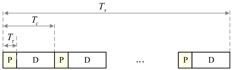
Figure 1: Superframe structure. “P” and “D” show pilot and data transmission phases. $T_{c}$ is the channel coherence time. $T_{s}$ is the superframe duration over which AoA and AoD remain unchanged, but the fast fading component of the channel changes per channel coherence time $T_{\tau}$.

As shown in Fig. 1, the signal transmission within each fading block consists of two phases: pilot transmission phase with duration $T_{\tau}$ and data transmission phase with duration $T_{d}=T_{c}-T_{\tau}$. In the following, we will elaborate on these phases.

II-B1 Pilot Transmission

To estimate the uplink channel, UE $k$ transmits pilot matrix $\mathbf{P}_{k}$ over $T_{\tau}$ channel uses. Let $\rho_{\tau}$ be the total energy devoted to the pilot transmission by each UE within each fading block, namely

$${\rm{tr}}\left(\mathbf{P}_{k}\mathbf{P}_{k}^{\mbox{\scriptsize H}}\right)=\rho_{\tau},\quad k=1,2,\ldots,K\>.$$ (6)

UE $k$ precodes its uplink pilots using spatial filter $\mathbf{V}_{k}$. The received signal at the BS is then combined using spatial filter $\mathbf{W}_{k}$ in order to estimate the corresponding channel. Collectively, the filtered received signal at the BS during the pilot transmission phase is

$$\mathbf{Y}_{\tau,k}=\mathbf{W}_{k}^{\mbox{\scriptsize H}}\sum_{j=1}^{K}\mathbf{H}_{j}\mathbf{V}_{j}\mathbf{P}_{j}+\mathbf{W}_{k}^{\mbox{\scriptsize H}}\mathbf{Z}_{\tau},$$ (7)

where $\mathbf{Z}_{\tau}\in\mathbb{C}^{M\times T_{\tau}}$ is the BS noise matrix with independent and identically distributed entries modeled as ${\rm{vec}}(\mathbf{Z}_{\tau})\sim\mathcal{CN}(\bm{0},\sigma_{z}^{2}\mathbf{I}_{MT_{\tau}})$. Note that $\mathbf{P}_{k}$ and $\mathbf{Y}_{\tau,k}$ have $T_{\tau}$ columns, while the number of rows depends on the dimensions of the spatial filters $\mathbf{V}_{k}$ and $\mathbf{W}_{k}$, respectively. In the next section, we will discuss pilot precoding and combining scenarios with different dimensions for the spatial filters.

II-B2 Data Transmission Phase

In this phase of the signal transmission, all the UEs transmit their precoded data symbols to the BS simultaneously. The data precoding filters are designed at the BS using the estimated channels and are fed back to the UEs through the feedback links. Each UE transmits its data symbols in $L$ streams over $T_{d}$ channel uses with constant average power $\rho_{d}/T_{d}$, where $\rho_{d}$ denotes the total energy devoted for data transmission by each UE within each fading block. We assume that the data symbols are independent and identically distributed as zero-mean circularly symmetric complex Gaussian random variables. Let $\mathbf{s}_{k}\in\mathbb{C}^{L}$ represent the data vector of UE $k$; then $\mathbf{s}_{k}\sim\mathcal{CN}(\mathbf{0},{\rho_{d}}/{T_{d}}\mathbf{I}_{L})$.

The data vector $\mathbf{s}_{k}$ is precoded before transmission using the linear spatial filter $\mathbf{F}_{k}\in\mathbb{C}^{N\times L}$. The received signal at the BS during the data transmission phase is

$$\mathbf{y}_{d}=\sum_{k=1}^{K}\mathbf{H}_{k}\mathbf{F}_{k}\mathbf{s}_{k}+\mathbf{z}_{d},$$ (8)

where $\mathbf{z}_{d}\sim\mathcal{CN}(\bm{0},\sigma_{z}^{2}\mathbf{I}_{M})$ is the thermal noise at the BS.

III Channel Estimation

In this section, we study the channel estimation quality for three different pilot transmission scenarios:

• non-precoded and uncombined pilot transmission (nPuC);

• precoded and uncombined pilot transmission (PuC); and

• precoded and combined pilot transmission (PC).

In the nPuC baseline scenario, every antenna element of every UE sends a unique pilot sequence (typically orthogonal to other pilot sequences). PuC allows precoding of the pilot signals at the transmitters (UEs in our case), but the receiver (BS) will not jointly process the signals received by its $M$ antenna elements. Finally, PC permits both precoders and combiners in the pilot transmission phase. Using (7) and Lemma 1 in Appendix A, the vectorized received signal in pilot transmission scenario $\mathtt{x}\in\{\text{nPuC},\text{PuC},\text{PC}\}$ is

$${\rm{vec}}\left(\mathbf{Y}_{\tau,k}^{(\mathtt{x})}\right)=\sum_{j=1}^{K}\left(\breve{\mathbf{P}}_{kj}^{(\mathtt{x})}\right)^{\mbox{\scriptsize H}}{\rm{vec}}\left(\mathbf{H}_{j}\right)+\breve{\mathbf{W}}_{k}{\rm{vec}}\left(\mathbf{Z}_{\tau}\right),$$ (9)

where $\big{(}\breve{\mathbf{P}}^{(\mathtt{x})}_{kj}\big{)}^{\mbox{\scriptsize H}}=\big{(}\mathbf{V}_{j}\mathbf{P}_{j}^{(\mathtt{x})}\big{)}^{\mathrm{\scriptsize T}}\otimes\mathbf{W}_{k}^{\mbox{\scriptsize H}}$ and $\breve{\mathbf{W}}_{k}=\mathbf{I}_{T_{\tau}}\otimes\mathbf{W}_{k}^{\mbox{\scriptsize H}}$.

In all the three scenarios, we use minimum mean squared error (MMSE) estimates of the channel, assuming that the spatial filters are known at the BS. Using [24, Equation (6)] and noting that the mean values of our channel matrices are zero, the MMSE estimate of channel $\mathbf{H}_{k}$ for scenario $\mathtt{x}$, can be expressed as

$${\rm{vec}}\!\left(\!\widehat{\mathbf{H}}_{k}^{(\mathtt{x})}\!\right)\!\!=\!\mathbf{R}_{k}\breve{\mathbf{P}}_{k}^{(\mathtt{x})}\!\!\left(\sum_{j=1}^{K}\!\left(\!\breve{\mathbf{P}}_{kj}^{(\mathtt{x})}\!\right)^{\!\!\mbox{\scriptsize H}}\mathbf{R}_{j}\breve{\mathbf{P}}_{kj}^{(\mathtt{x})}\!+\!\sigma_{z}^{2}\breve{\mathbf{W}}_{\!k}\!\right)^{\!\!\!\!-1}\!\!\!\!\!{\rm{vec}}\!\left(\!\mathbf{Y}_{\tau,k}^{(\mathtt{x})}\!\right),$$ (10)

where $\breve{\mathbf{P}}^{(\mathtt{x})}_{k}=\breve{\mathbf{P}}^{(\mathtt{x})}_{kk}$.

In the rest of this section, we drive the channel estimate in each pilot transmission scenario. Based on these derivations, we will then analyze and compare the channel estimation performance in the studied scenarios.

III-A Non-precoded and Uncombined Pilot Transmission (nPuC)

In the first pilot transmission scenario, used as a benchmark, orthogonal training sequences are transmitted from the different UEs’ antenna elements[8]. Moreover, in this scenario, neither pilot precoding at the UEs nor pilot combining at the BS is performed. On the positive side, this scenario requires no prior information about the channel. On the negative side, this traditional scheme requires at least $T_{\tau}^{(\text{nPuC})}=KN$ resource elements for the pilot transmission phase, which can grow large as the number of antenna elements per UE increases, e.g., in mmWave networks [25]. Moreover, the lack of transmit/receive antenna gains reduces SNR of individual pilots, decreasing the channel estimation quality, which negatively affects the data precoding performance of the BS and UEs. Therefore, nPuC does not meet any of the pilot transmission criteria that we mentioned earlier, i.e., scalability and balanced data-pilot coverage. Considering the pilot energy constraint (6), we have

$$\mathbf{P}_{k}^{(\text{nPuC})}\left(\mathbf{P}_{j}^{(\text{nPuC})}\right)^{\mbox{\scriptsize H}}=\begin{cases}\frac{\rho_{\tau}}{N}\mathbf{I}_{N}&k=j\>,\\ \bm{0}&\mbox{otherwise}\>,\end{cases}$$ (11)

where $\mathbf{P}_{k}^{(\text{nPuC})}\in\mathbb{C}^{N\times KN}$ is the pilot matrix transmitted from UE $k$ in scenario nPuC. Substituting the pilot symbols of (11) and replacing the spatial filters by identity matrices in (10), the MMSE estimate of the vectorized channel is

$$\begin{split}{\rm{vec}}\left(\widehat{\mathbf{H}}_{k}^{(\text{nPuC})}\right)=&\mathbf{R}_{k}\breve{\mathbf{P}}^{(\text{nPuC})}_{k}\left(\!\!\left(\!\breve{\mathbf{P}}^{(\text{nPuC})}_{k}\!\right)^{\!\!\mbox{\scriptsize H}}\!\mathbf{R}_{k}\breve{\mathbf{P}}^{(\text{nPuC})}_{k}\!\!+\!\sigma_{z}^{2}\mathbf{I}\!\right)^{\!\!\!-1}\\ &\hskip 14.22636pt\cdot{\rm{vec}}\left(\mathbf{Y}_{\tau}^{(\text{nPuC})}\right),\end{split}$$ (12)

where $\breve{\mathbf{P}}_{k}^{(\text{nPuC})}=\big{(}\mathbf{P}_{k}^{(\text{nPuC})}\big{)}^{*}\otimes\mathbf{I}_{M}$. Note that $\{\breve{\mathbf{P}}_{k}^{(\text{nPuC})}\}_{k=1}^{K}$ inherit the orthogonality property of $\{\mathbf{P}_{k}^{(\text{nPuC})}\}_{k=1}^{K}$, and therefore the signals received from UE $j\neq k$ can be canceled out in the process of channel estimation for UE $k$.

Define the estimation error matrix of scenario nPuC by ${\widetilde{\mathbf{H}}^{(\text{nPuC})}_{k}=\mathbf{H}_{k}-\widehat{\mathbf{H}}^{(\text{nPuC})}_{k}}$. Then, in the following proposition, we find its covariance under the traditional non-precoded uncombined pilot transmission scenario:

Proposition 1.

Consider the system model of scenario nPuC. Suppose that the channel is estimated with orthogonal pilots given by (11) and an MMSE estimator given by (12). The covariance matrix of the channel estimation error is

$$\begin{split}\widetilde{\mathbf{R}}_{k}^{(\text{nPuC})}&=\mathbb{E}\left[{{\rm{vec}}\left(\widetilde{\mathbf{H}}^{(\text{nPuC})}_{k}\right)}{{\rm{vec}}\left(\widetilde{\mathbf{H}}^{(\text{nPuC})}_{k}\right)}^{\mbox{\scriptsize H}}\right]\\ &=\delta M\sigma^{2}_{k}\left(\mathbf{U}_{k}^{*}\odot\mathbf{B}_{k}\right)\\ &~{}~{}~{}\cdot\left(\mathbf{I}_{L}\!+\!M\zeta_{k}\left(\mathbf{R}_{\mathbf{U}_{k}}^{\mathrm{\scriptsize T}}\!\circ\!\mathbf{R}_{\mathbf{B}_{k}}\right)\right)^{\!\!-1}\!\left(\mathbf{U}_{k}^{*}\!\odot\!\mathbf{B}_{k}\right)^{\mbox{\scriptsize H}},\end{split}$$ (13)

where $\mathbf{R}_{\mathbf{U}_{k}}=\mathbf{U}_{k}^{\mbox{\scriptsize H}}\mathbf{U}_{k}$, $\mathbf{R}_{\mathbf{B}_{k}}=\mathbf{B}_{k}^{\mbox{\scriptsize H}}\mathbf{B}_{k}$,

$$\zeta_{k}=\frac{\rho_{\tau}\sigma^{2}_{k}}{L\sigma_{z}^{2}},$$ (14)

and the expectation is taken over the distribution of the random channel and the received noise.

Proof:

A proof is given in Appendix B. ∎

The following proposition characterizes the normalized mean square error (MSE) in scenario nPuC as an indicator of the channel estimation quality.

Proposition 2.

Consider the covariance of the MMSE channel estimation error in Proposition 1. The corresponding normalized MSE, $e_{k}^{(\text{nPuC})}={\rm{tr}}(\widetilde{\mathbf{R}}_{k}^{(\text{nPuC})})/{\rm{tr}}(\mathbf{R}_{k})$, is bounded as

$$\frac{1}{1+M\zeta_{k}}\left[1-\frac{\epsilon_{k}^{(\text{nPuC})}}{M\zeta_{k}}\right]^{\!+}\!\!\leq e_{k}^{(\text{nPuC})}\!\leq\!\frac{1}{1+M\zeta_{k}}\;,$$ (15)

where

$$\epsilon_{k}^{(\text{nPuC})}=\frac{\left(1-\kappa\left(\mathbf{I}_{L}+M\zeta_{k}\;\mathbf{R}_{\mathbf{U}_{k}}^{\mathrm{\scriptsize T}}\circ\mathbf{R}_{\mathbf{B}_{k}}\right)\right)^{2}}{4\kappa\left(\mathbf{I}_{L}+M\zeta_{k}\;\mathbf{R}_{\mathbf{U}_{k}}^{\mathrm{\scriptsize T}}\circ\mathbf{R}_{\mathbf{B}_{k}}\right)}\geq 0\>,$$

and $\left[a\right]^{+}=\max(a,0)$ for $a\in\mathbb{R}$.

Corollary 1.

As $N\to\infty$ (so $\mathbf{R}_{\mathbf{U}_{k}}\to\mathbf{I}_{L}$), both upper and lower bounds in (15) become tight in the sense that

$$e_{k}^{(\text{nPuC})}\to(1+M\zeta_{k})^{-1}.$$ (16)

(a) Network with $M=8$.

(b) Network with $M=1024$.

Figure 2: The channel estimation performance in non-precoded and uncombined pilot transmission scenario (nPuC) as a function of the number of UEs antennas $N$. $M=8$ and $M=1024$ represent cellular networks with small and large number of BS antennas, respectively. The dashed lines represent the bounds of Proposition 2 for the corresponding average normalized MSE curves; however, some of the bounds are tight and can not be seen in the figure.

To numerically illustrate Proposition 2, we simulate a network with various number of UE antenna elements $N$, paths $L$, and BS antenna elements $M$. The channel model follows (1). Our simulation parameters cover wide range of use cases, including

• Access layer of traditional cellular or ad hoc networks (small $N$, small $M$, large $L$);

• Access layer of sub-6 GHz massive MIMO networks (small $N$, large $M$, large $L$); and

• Access layer of mmWave networks (small $N$, large $M$, small $L$); and

• Backhaul layer (large $N$ and $M$ values, small or large $L$).

We draw the AoAs and AoDs independently from uniform distributions in $[-{\pi}/{3},{\pi}/{3}]$ and $[-{\pi}/{6},{\pi}/{6}]$, respectively. The normalized MSE is averaged over 50 realizations of AoAs and AoDs and 90,000 realizations of noise and small-scale fading. We consider $\rho_{\tau}=0$ dB and apply the normalization $\sigma^{2}_{k}/\sigma_{z}^{2}=1$ to ensure that the average received SNR at the BS can be described by the pilot energy and the number of antenna elements, e.g., $\text{SNR}={\rho_{\tau}}/{N}$ in nPuC.

Fig. 2 illustrates the average normalized MSE, $e_{k}^{(\text{nPuC})}$ as defined in Proposition 2, against the number of antenna elements at UE $k$ for $M=8,1024$ (as small and large numbers) and three different number of paths between the UE and the BS, namely $L=2,4,8$. These numbers of multipath components cover both sparse scattering environments like in mmWave networks and rich scattering environments like in sub-6 GHz networks. Fig. 2 shows that increasing $N$ does not improve the channel estimation performance of nPuC. The reason for this becomes clear by noting that the MMSE channel estimation error is proportional to the dimension of the received signal vector, i.e., ${\rm{vec}}\left(\mathbf{Y}_{\tau}^{(\text{nPuC})}\right)\in\mathbb{C}^{KNM}$, as well as the received SNR. On one hand, increasing $N$ linearly increases the dimension of the received signal. These extra observations, while having a constant number of unknown parameters, generally improve the channel estimation performance. On the other hand, increasing $N$ reduces the received SNR, formulated in the previous paragraph. These two effects cancel each other, making the average normalized MSE almost independent of the number of UE antennas $N$. On the contrary, comparing Fig. 2(a) and Fig. 2(b) shows that adding more antenna elements to the BS enhances the channel estimation performance. This can also be related to the increase in the dimension of the received signal by increasing the number of BS antennas, $M$. Another observation from Fig. 2 is that the channel estimation performance improves for networks with sparser scattering environments (smaller $L$), where this improvement is almost linear in the large antenna regimes; see Corollary 1.

III-B Precoded and Uncombined Pilot Transmission (PuC)

In the second pilot transmission scenario, the pilots are precoded using spatial filters at the UEs. However, no pilot combining is performed at the BS. The channel estimation quality in this scenario depends on the statistical information of the channel available prior to pilot transmission. Assuming that $\mathbf{U}_{k}$ is available at UE $k$, either perfectly or with some unbiased errors[26], the spatial filters can be designed to help focusing the pilot energy along the strongest multipath components between the UEs and the BS. Hence, precoding the pilots boosts the SNR in the pilot transmission phase, which is specially beneficial for the UEs at the cell edges.

Considering that there are $L\leq N$ paths between each UE and the BS, $T_{\tau}^{(\text{PuC})}=KL\leq T_{\tau}^{(\text{nPuC})}$ pilot symbols suffices for transmitting orthogonal training sequences through all the paths. In other words, unlike scenario nPuC, where orthogonal pilots are assigned to the UE antennas, the number of required orthogonal pilot sequences in scenario PuC is equal to the number of multipath components. Clearly, this pilot transmission scheme leaves longer time for the data transmission phase, compared to the baseline scenario nPuC. This brings a significant gain for the data transmission time, especially in wireless networks with small coherence time such as mmWave networks [14].

Let $\mathbf{P}_{k}^{(\text{PuC})}\in\mathbb{C}^{L\times T_{\tau}^{(\text{PuC})}}$ be the pilot symbols transmitted by UE $k$ in scenario PuC, then orthogonality of training sequences and the energy constraint (6) imply that

$$\mathbf{P}_{k}^{(\text{PuC})}\left(\mathbf{P}_{j}^{(\text{PuC})}\right)^{\mbox{\scriptsize H}}=\begin{cases}\frac{\rho_{\tau}}{L}\mathbf{I}_{L}&k=j\>,\\ \bm{0}&\mbox{otherwise}\>.\end{cases}$$ (17)

Note that although in this paper we are investigating the uplink channel estimation, pilot transmission scenario PuC entails the same complexity for downlink channel estimation. In contrast, the complexity of the downlink channel estimation in scenario nPuC is substantially higher than that of uplink channel estimation if $M\gg KN$. As a result, in massive MIMO systems, the nPuC scheme is suitable only for the TDD mode (in which the channel reciprocity principle holds), whereas PuC can be used in both TDD and FDD modes. Note that the number of unique pilots required by PuC does still scale by the number of UEs. Moreover, due to the lack of receiver antenna gain, it may not completely solve the imbalanced pilot-data coverage problem, though substantially alleviate it compared to the nPuC scheme.

For mathematical tractability, we assume the availability of of perfect second-order statistics information which allows us to gain insights about the impact of different parameters on the network performance (e.g., channel estimation quality and network throughput). In this section, we choose the precoding matrix $\mathbf{V}_{k}=\mathbf{U}_{k}$ for each UE $k$, which simplifies the mathematical analysis and, at the same time, is asymptotically optimal in terms of maximizing the SNR [27]. No combining filter is considered at the BS in this scenario, that is $\mathbf{W}_{k}=\mathbf{I}_{M}$. Substituting the training matrix and spatial filters of scenario PuC into (10), the MMSE estimate of the channel becomes

$${\rm{vec}}\left(\widehat{\mathbf{H}}_{k}^{(\text{PuC})}\right)=\, \mathbf{R}_{k}\breve{\mathbf{P}}^{(\text{PuC})}_{k}\left(\left(\breve{\mathbf{P}}^{(\text{PuC})}_{k}\right)^{\mbox{\scriptsize H}}\mathbf{R}_{k}\breve{\mathbf{P}}^{(\text{PuC})}_{k}+\sigma_{z}^{2}\mathbf{I}\right)^{-1}$$

$$\cdot{\rm{vec}}\left(\mathbf{Y}_{\tau}^{(\text{PuC})}\right),$$ (18)

where $\breve{\mathbf{P}}^{(\text{PuC})}_{k}=\big{(}\mathbf{U}_{k}\mathbf{P}_{k}^{(\text{PuC})}\big{)}^{*}\otimes\mathbf{I}_{M}$. $\{\breve{\mathbf{P}}^{(\text{PuC})}_{k}\}_{k=1}^{K}$ inherit the orthogonality property of $\{\mathbf{P}^{(\text{PuC})}_{k}\}_{k=1}^{K}$, similar to nPuC, and therefore the received signals from UE $j\neq k$ are canceled out at the receiver in the estimation process of $\mathbf{H}_{k}$.

Define the estimation error matrix as $\widetilde{\mathbf{H}}_{k}^{(\text{PuC})}=\mathbf{H}_{k}-\widehat{\mathbf{H}}_{k}^{(\text{PuC})}$. The following propositions characterize the accuracy of the channel estimation under precoded but uncombined pilot transmission:

Proposition 3.

Consider the system model of scenario PuC. The covariance of the channel estimation error matrix using orthogonal pilot transmissions given by (17) and an MMSE estimator given by (III-B) is

$$\begin{split}{\widetilde{\mathbf{R}}}_{k}^{(\text{PuC})}\!\!&=\mathbb{E}\left[{\rm{vec}}\left(\widetilde{\mathbf{H}}^{(\text{PuC})}_{k}\right){\rm{vec}}\left(\widetilde{\mathbf{H}}^{(\text{PuC})}_{k}\right)^{\mbox{\scriptsize H}}\right]\\ &=\delta M\sigma^{2}_{k}\left(\mathbf{U}_{k}^{*}\odot\mathbf{B}_{k}\right)\\ &~{}~{}~{}\cdot\left(\mathbf{I}_{L}\!+\!\delta M\zeta_{k}\left(\mathbf{R}_{\mathbf{U}_{k}}^{2}\right)^{\mathrm{\scriptsize T}}\!\!\circ\!\mathbf{R}_{\mathbf{B}_{k}}\!\right)^{\!\!-1}\!\!\left(\mathbf{U}_{k}^{*}\!\odot\!\mathbf{B}_{k}\right)^{\mbox{\scriptsize H}}.\end{split}$$ (19)

Proof:

A proof is given in Appendix B. ∎

Proposition 4.

Consider the covariance of the channel estimation error for UE $k$ given by Proposition 3. The normalized MSE, defined as $e_{k}^{(\text{PuC})}={\rm{tr}}(\widetilde{\mathbf{R}}_{k}^{(\text{PuC})})/{\rm{tr}}(\mathbf{R}_{k})$, is bounded as

$$\frac{\lambda_{\max}^{-1}}{1\!+\!\delta M\zeta_{k}}\!\left[1\!-\!\frac{\epsilon_{k}^{(\text{PuC})}}{\delta M\zeta_{k}}\right]^{\!+}\!\!\!\leq\!e_{k}^{(\text{PuC})}\!\leq\!\frac{\lambda_{\min}^{-1}}{1\!+\!\delta M\zeta_{k}},$$ (20)

where $\lambda_{\min}$ and $\lambda_{\max}$ represent the minimum and maximum eigenvalues of $\mathbf{R}_{\mathbf{U}_{k}}$, respectively and

$$\epsilon_{k}^{(\text{PuC})}=\frac{\left(1-\kappa\left(\mathbf{I}_{L}+\delta M\zeta_{k}\left(\mathbf{R}_{\mathbf{U}_{k}}^{2}\right)^{\mathrm{\scriptsize T}}\circ\mathbf{R}_{\mathbf{B}_{k}}\right)\right)^{2}}{4\kappa\left(\mathbf{I}_{L}+\delta M\zeta_{k}\left(\mathbf{R}_{\mathbf{U}_{k}}^{2}\right)^{\mathrm{\scriptsize T}}\circ\mathbf{R}_{\mathbf{B}_{k}}\right)}\geq 0.$$ (21)

Corollary 2.

As $N\to\infty$ (so $\mathbf{R}_{\mathbf{U}_{k}}\to\mathbf{I}_{L}$), both upper and lower bounds in (20) become tighter, and ${e_{k}^{(\text{PuC})}\to(1+\delta M\zeta_{k})^{-1}}$.

Corollaries 1 and 2 characterize the estimation error in scenarios nPuC and PuC, respectively. In particular, when $N\to\infty$, pilot precoding can improve the channel estimation error by a factor of

$$\lim_{N\to\infty}\frac{e_{k}^{(\text{PuC})}}{e_{k}^{(\text{nPuC})}}=\dfrac{1+M\zeta_{k}}{1+\delta M\zeta_{k}}\geq\frac{1}{\delta}\>,$$ (22)

where the equality holds if $M\zeta_{k}$ is sufficiently large. The proof of (22) is a straightforward application of Lemma 5 in Appendix A.

(a) Network with $M=8$.

(b) Network with $M=1024$.

Figure 3: The channel estimation performance in the precoded uncombined pilot transmission scenario (PuC) as a function of the number of UEs antenna elements. $M=8$ and $M=1024$ represent cellular networks with small and large number of BS antennas, respectively. The dashed lines represent the bounds of Proposition 4 for the corresponding average normalized MSE curves.

To numerically evaluate the performance of channel estimation using PuC, we use the same simulation setting as the one used in Fig. 2. The average normalized MSE and the corresponding bounds, as computed in (20), against the number of antenna elements at the UEs are illustrated in Fig. 3 for three different values of $L$, namely $L=2,4,8$. As the figure shows, unlike nPuC, increasing $N$ significantly boosts the channel estimation performance. Moving from $N=8$ to $N=1024$ reduces the estimation error by around 20 dB. The reason is that in PuC, as $N$ grows large, the energy transmitted through the paths between the UEs and the BS increases. Therefore, unlike nPuC, the received SNR at the BS in PuC increases with $N$. Again, similarly to nPuC, by comparing Fig. 3(a) and Fig. 3(b), we can see that when $M$ increases from 8 to 1024, a gain of $10\log_{10}({1024}/{8})\approx 21$ dB can be achieved.

The gain of pilot precoding in PuC can be understood by comparing Fig. 2 and Fig. 3. Specifically, when the number of antenna elements at both the UE and BS sides is large, say $M=N=1024$, Fig. 3(b) shows 21, 24 and 27 dB lower MSE compared with Fig. 2(b) for the curves corresponding to $L=2,4$ and $8$, respectively. This fact is in accordance with (22).

III-C Precoded and Combined Pilot Transmission (PC)

In the third scenario, in addition to precoding the pilots at UEs, the received signals at the BS are also combined, using the available information about the AoAs at the BS. In this case, in addition to the gains discussed earlier for PuC, exploiting the spatial filters at the BS, given the large number of BS antennas, can lead to a sufficiently good spatial separation of the UEs. Therefore, a combiner at the BS may enable us to use non-orthogonal pilots for different UEs, if their orthogonality can be maintained in the spatial domain. Therefore, in this scenario, non-orthogonal sequences with $T_{\tau}^{(\text{PC})}<KL$ symbols are transmitted from each antenna elements. Without loss of generality, we consider the extreme scenario of $T_{\tau}^{\text{PC}}=1$ in our mathematical analysis, that is only one pilot will be used to estimate the entire uplink channel matrix. Due to the pilot reuse, there is a contamination of the pilots at the BS side. This situation is similar to a multi-cell network where pilot reuse in neighboring cells causes the pilot contamination problem. Notice that scenario PC addresses the pilot contamination problem, though we have a single cell network setting. We then show with numerical analysis that using $T_{\tau}^{\text{PC}}>1$ orthogonal pilots brings improvement in the channel estimation performance at the expense of having less time for the data transmission phase. Notice that, similarly to PuC, pilot transmission scenario PC enables the realization of massive MIMO using both TDD and FDD schemes, as the channel estimation complexity grows only with the number of paths, rather than with the number of antennas, which is a useful property for both UL and DL pilots. Altogether, PC with $1\leq T_{\tau}^{\text{PC}}<KL$ pilots is a promising option that not only scales well with the number of UEs but also eliminates the imbalanced pilot-data coverage problem.

We assume that $\mathbf{U}_{k}$ is available at UE $k$ and all the $\mathbf{U}_{k}$’s and $\mathbf{B}_{k}$’s are available at the BS either perfectly or with some unbiased error. In the rest of this section for the sake of mathematical tractability, we assume that the knowledge about the AoAs and AoDs at the BS and UEs is perfect. Later, using numerical simulations, we investigate the effect of imperfect knowledge about AoAs and AoDs on the performance of the network. Exploiting the available information about the channel, similarly to PuC, the pilot precoding filter at UE $k$ is designed as $\mathbf{V}_{k}=\mathbf{U}_{k}$. Moreover, recalling that the main objective of this paper is to characterize the gains of pilot precoding/combining rather than finding the optimal precoders and combiners, we design the combining filter for UE $k$ as $\mathbf{W}_{k}=\mathbf{B}_{k}$.

Substituting for the spatial filters in (9), the received signal in scenario PC is

$$\begin{split}{\rm{vec}}\!\left(\mathbf{Y}^{(\text{PC})}_{\tau,k}\right)\!&=\!\left(\!\breve{\mathbf{P}}^{(\text{PC})}_{k}\!\right)^{\mbox{\scriptsize H}}\!\!{\rm{vec}}\left(\mathbf{H}_{k}\right)\!+\!\left(\mathbf{I}\!\otimes\!\mathbf{B}_{k}^{\mbox{\scriptsize H}}\right){\rm{vec}}\left(\mathbf{Z}_{\tau}\right)\\ &~{}~{}~{}+\underbrace{\sum\limits_{j=1,j\neq k}^{K}\!\left(\!\breve{\mathbf{P}}^{(\text{PC})}_{kj}\!\right)^{\mbox{\scriptsize H}}\!\!{\rm{vec}}\left(\mathbf{H}_{j}\right)}_{\text{Inter-UE Interference}}\>,\end{split}$$ (23)

where $\big{(}\breve{\mathbf{P}}^{(\text{PC})}_{kj}\big{)}^{\mbox{\scriptsize H}}=\big{(}\mathbf{U}_{j}\mathbf{P}_{j}^{(\text{PC})}\big{)}^{\mathrm{\scriptsize T}}\otimes\mathbf{B}_{k}^{\mbox{\scriptsize H}}$ with $\mathbf{P}^{(\text{PC})}_{j}\in\mathbb{C}^{L\times T_{\tau}^{(\text{PC})}}$ being the pilot matrix transmitted from UE $j$.

Unlike the two previous scenarios, in PC, pilot contamination is inevitable due to non-orthogonal pilot transmissions. In fact, pilot contamination may contain two parts: the interference from pilots transmitted from the antenna elements of the same UE, called intra-UE interference, and the interference from the pilots transmitted from other UEs, called inter-UE interference. Note that, in the case of multicell networks, the interference from the UEs in other cells, called inter-cell interference, can also contaminate the received pilots. The pilot precoding used in this scenario is beneficial for boosting the link budget and reducing the inter-UE interference while the pilot combining mitigates both inter-UE and inter-cell interferences.

Define the covariance matrix of the inter-UE interference term and the covariance of the received signal without inter-UE interference respectively by

$$\macc@depth\char 1\relax\frozen@everymath{\macc@group}\macc@set@skewchar\macc@nested@a 111 =\sum\limits_{j=1,j\neq k}^{K}\left(\breve{\mathbf{P}}^{(\text{PC})}_{kj}\right)^{\!\!\mbox{\scriptsize H}}\mathbf{R}_{j}\breve{\mathbf{P}}^{(\text{PC})}_{kj}\;,$$ (24)

$$\mathbf{Q}_{k} =\left(\breve{\mathbf{P}}^{(\text{PC})}_{k}\right)^{\!\!\mbox{\scriptsize H}}\mathbf{R}_{k}\breve{\mathbf{P}}^{(\text{PC})}_{k}+\sigma_{z}^{2}\left(\mathbf{I}\otimes\mathbf{R}_{\mathbf{B}_{k}}\right).$$ (25)

It is now straightforward to show that the MMSE estimate of the vectorized channel in this scenario is

$$\begin{split}{\rm{vec}}\left(\widehat{\mathbf{H}}_{k}^{(\text{PC})}\right)=\mathbf{R}_{k}\breve{\mathbf{P}}^{(\text{PC})}_{k}\left(\mathbf{Q}_{k}+\macc@depth\char 1\relax\frozen@everymath{\macc@group}\macc@set@skewchar\macc@nested@a 111{}_{k}\right)^{-1}{\rm{vec}}\left(\mathbf{Y}^{(\text{PC})}_{\tau,k}\right).\end{split}$$ (26)

Let $\widetilde{\mathbf{H}}_{k}^{(\text{PC})}=\mathbf{H}_{k}-\widehat{\mathbf{H}}_{k}^{(\text{PC})}$ be the error due to estimating channel ${\mathbf{H}}_{k}$ in the PC scenario. Then,

$$\begin{split}\widetilde{\mathbf{R}}_{k}^{(\text{PC})}&=\mathbb{E}\left[{\rm{vec}}\left(\widetilde{\mathbf{H}}_{k}^{(\text{PC})}\right){\rm{vec}}\left(\widetilde{\mathbf{H}}_{k}^{(\text{PC})}\right)^{\mbox{\scriptsize H}}\right]\\ &=\mathbf{R}_{k}-\mathbf{R}_{k}\breve{\mathbf{P}}^{(\text{PC})}_{k}\left(\mathbf{Q}_{k}+\macc@depth\char 1\relax\frozen@everymath{\macc@group}\macc@set@skewchar\macc@nested@a 111{}_{k}\right)^{-1}\left(\breve{\mathbf{P}}^{(\text{PC})}_{k}\right)^{\mbox{\scriptsize H}}\mathbf{R}_{k}\>.\end{split}$$ (27)

(a) Network with $M=8$.

(b) Network with $M=1024$.

Figure 4: Channel estimation performance in the precoded and combined pilot transmission scenario (PC) as a function of the number of UEs antenna elements with $T_{\tau}=L$ and $T_{\tau}=1$ training lengths. $M=8$ and $M=1024$ represent cellular networks with small and large number of BS antennas, respectively.

From (27), we have the following useful corollary:

Corollary 3.

In PC, the pilot contamination caused by inter-UE and intra-UE interference tend to zero, when the number antenna elements at the BS and UEs grow large, respectively.

Proof:

A proof is given in Appendix B. ∎

Corollary 3 implies that the combiner substantially reduces the pilot contamination term, and asymptotically makes it zero. It is straightforward to show that Corollary 3 holds also for multicell networks, and only one pilot in the asymptotic regime is enough for channel estimation in the entire network.

In the non-asymptotic case, using more orthogonal pilots per UE allows to reduce the number of antennas contributing to the pilot contamination term and to maintain the UE’s transmit power under a desirable threshold. Finding the minimum number of orthogonal pilots for a given maximum power of the pilot contamination is an interesting topic for future works.

We use the same simulation setting as that of Fig. 2 to analyze the performance of PC. However, in this scenario, all the UEs are transmitting the same pilot symbols, which leads to inter-UE interference at the BS. When $T_{\tau}\geq N$, the orthogonal pilots are assigned to difference antenna elements of one UE to avoid intra-UE interference. When $T_{\tau}<N$, the intra-UE interference is inevitable and, in the extreme case when $T_{\tau}=1$, all the antenna elements of UEs transmit the same pilot symbols, and therefore interfere at the BS. For the sake of simplicity, we also assume that all the UEs are located at the same distance from the BS and therefore experience the same path loss.

Fig. 4 illustrates the average normalized MSE against the number of antenna elements at the UEs for a network with $K=2$ UEs. This figure manifests similar behaviors as of Fig. 3, such as better channel estimate with higher $N$, higher $M$, and lower $L$. Moreover, comparing Fig. 4(a) to Fig. 4(b) reveals that more antenna elements at the BS increases separability of different UEs in the spatial domain, so makes it possible to use smaller number of unique pilots for a given power for the pilot contamination term. In particular, with $M=8$, the inter-UE interference term of the pilot contamination is so strong that additional interference and the corresponding SINR loss due to pilot reuse within one UE (namely $T_{\tau}<L$) may not be tolerable and leads to substantial loss in the performance of channel estimation. However, when $M=1024$, the inter-UE interference term is almost negligible, making intra-UE interference tolerable for a given minimum SINR threshold for the received pilot signal.

Figure 5: Channel estimation performance in the precoded and combined pilot transmission scenario (PC) as a function of number of UEs in the cell.

The pilot contamination effect on the channel estimation performance is investigated in Fig. 5. This figure illustrates the average normalized MSE against the number of UEs in the cell for a network with $M=128$, $N=32$ and $L=4$. For the sake of simplicity, all the UEs are located at the same distance from the BS and therefore experience the same path loss. The AoDs and AoAs are drawn independently from uniform random distributions in $[-\pi/6,\pi/6]$ and $[-\pi/3,\pi/3]$, respectively. The results are averaged over 50 different realizations of AoAs and AoDs. Two pilot sequence length, namely $T_{\tau}=4,1$, are considered in this figure. In the case of $T_{\tau}=4$, no intra-UE interference exists, and only the inter-UE interference degrades the channel estimation performance when $K$ increases. However, when $T_{\tau}=1$ both intra-UE and inter-UE interference contaminate the pilot symbols which leads to at least 5 dB poorer performance compared to the case when $T_{\tau}=4$.

Fig. 6 shows the average normalized MSE against the total pilot transmission power using the same setup as in Fig. 5 when there are $K=2$ UEs in the network. According to this figure, pilot precoding with $N=32$ can achieve the same estimation error as nPuC with almost 5 dB less power. Alternatively, for a given total pilot transmission power, pilot precoding can improve the estimation error by 6 dB compared with the conventional nPuC. Moreover, the performance of PC with only 4 orthogonal pilots is almost identical to that of PuC with 64 orthogonal pilots. In other words, these 16 x shorter training length allows channel estimation of substantially higher number of UEs within the same coherence budget, while also leaving more time for the data transmission. Therefore, in PC we expect a boost in the achievable rate with 4 orthogonal pilots compared to that of PuC.

Figure 6: The impact of pilot energy and number of transmitted pilot symbols on the channel estimation performance in the three pilot transmission scenarios.

So far, we have analyzed the channel estimation quality of three pilot transmission scenarios. In the next section, we investigate their effects on the achievable data rate.

IV Data Transmission

In this section, we study the sum-rate of the multiple access channel between the UEs and the BS in the uplink data transmission phase. Denoting the transmitted signal vector of UE $k$ by $\mathbf{x}_{k}=\mathbf{F}_{k}\mathbf{s}_{k}$, (8) can be equivalently written as

$$\begin{split}\mathbf{y}_{d}=\sum_{k=1}^{K}\mathbf{H}_{k}\mathbf{x}_{k}+\mathbf{z}_{d}=\sum_{k=1}^{K}\widehat{\mathbf{H}}_{k}\mathbf{x}_{k}+\underbrace{\sum_{k=1}^{K}\widetilde{\mathbf{H}}_{k}\mathbf{x}_{k}+\mathbf{z}_{d}}_{\mathbf{z}_{\text{eff}}}\>,\end{split}$$ (75)

where $\mathbf{z}_{\text{eff}}$ is the effective noise at the BS which combines the receiver noise and the residual channel estimation errors.

In the following, we first present the performance metric used for the performance evaluation of the network. Subsequently, we study the precoding methods that are used in the data transmission phase.

IV-A Performance Metric

Although the optimal distribution of $\{\mathbf{x}_{k}\}_{k=1}^{K}$ is not known, using (75), the following lower bound for the sum-rate of the network can be found as [28]:

$$\begin{split}r&=\frac{T_{d}}{T_{c}}\mathbb{E}\left[\log\det\left(\mathbf{I}_{M}+\mathbf{R}_{\mathbf{z}_{\text{eff}}}^{-1}\sum_{k=1}^{K}\widehat{\mathbf{H}}_{k}\mathbf{R}_{\mathbf{x}_{k}}\widehat{\mathbf{H}}_{k}^{\mbox{\scriptsize H}}\right)\right],\end{split}$$ (76)

where $\mathbf{R}_{\mathbf{x}_{k}}$ and $\mathbf{R}_{\mathbf{z}_{\text{eff}}}$ are the covariance matrices of $\mathbf{x}_{k}$ and $\mathbf{z}_{\text{eff}}$, respectively, and are defined as

$$\mathbf{R}_{\mathbf{x}_{k}} =\mathbb{E}\left[\mathbf{x}_{k}\mathbf{x}_{k}^{\mbox{\scriptsize H}}\right]=\mathbf{F}_{k}\mathbb{E}\left[\mathbf{s}_{k}\mathbf{s}_{k}^{\mbox{\scriptsize H}}\right]\mathbf{F}_{k}^{\mbox{\scriptsize H}}=\frac{\rho_{d}}{T_{d}}\mathbf{F}_{k}\mathbf{F}_{k}^{\mbox{\scriptsize H}}\>,$$ (77)

$$\mathbf{R}_{\mathbf{z}_{\text{eff}}} =\mathbb{E}\left[\mathbf{z}_{\text{eff}}\mathbf{z}_{\text{eff}}^{\mbox{\scriptsize H}}\right]=\sum_{k=1}^{K}\mathbb{E}\left[\widetilde{\mathbf{H}}_{k}\mathbf{R}_{\mathbf{x}_{k}}\widetilde{\mathbf{H}}_{k}^{\mbox{\scriptsize H}}\right]+\sigma_{z}^{2}\;\mathbf{I}_{M}.$$ (78)

IV-B Data Precoding

For a single link MIMO network, when only imperfect CSI is available at the transmitter, it is shown that the eigenvectors of the channel estimate covariance matrix represent the optimal transmit directions [29, Theorem 1]. More specifically, the precoder of UE $k$ is designed in a way that its signal is transmitted in the direction of the right singular vectors of the estimated channel matrix $\widehat{\mathbf{H}}_{k}$. For the sake of simplicity, we choose to allocate equal powers to different eigendirections for all three pilot precoding scenarios. Note that considering optimal power allocation does not change the insights that we gain from the comparative performance analysis of this paper, but complicates the mathematical analysis; see [29] for the optimal power allocation algorithm. Formally, denote the eigen-value decomposition of $\mathbf{R}_{\mathbf{x}_{k}}$ by $\mathbf{R}_{\mathbf{x}_{k}}=\bar{\mathbf{F}}_{k}\mathbf{\Lambda}_{k}\bar{\mathbf{F}}_{k}^{\mbox{\scriptsize H}}$ and that of $\widehat{\mathbf{H}}_{k}^{\mbox{\scriptsize H}}\widehat{\mathbf{H}}_{k}$ by $\widehat{\mathbf{H}}_{k}^{\mbox{\scriptsize H}}\widehat{\mathbf{H}}_{k}=\mathbf{E}_{k}\mathbf{\Sigma}_{k}\mathbf{E}_{k}^{\mbox{\scriptsize H}}$. Here, we set $\bar{\mathbf{F}}_{k}=\mathbf{E}_{k}$ and $\mathbf{\Lambda}_{k}=\rho_{d}/(T_{d}L)\mathbf{T}_{L}$ where $\mathbf{T}_{L}$ is a diagonal matrix whose first $L$ diagonal elements are one and the rest are zero. Comparing the designed covariance matrix of the data signal with the one in (77), the data precoding matrix corresponding to UE $k$ is found as

$$\mathbf{F}_{k}=\sqrt{\frac{1}{L}}\;\bar{\mathbf{F}}_{k}\mathbf{T}_{L}=\sqrt{\frac{1}{L}}\;\mathbf{E}_{k}\mathbf{T}_{L}\>.$$ (79)

(a) Total energy $\rho_{\tau}+\rho_{d}=0.1$.

(b) Total energy $\rho_{\tau}+\rho_{d}=0.5$.

Figure 7: Spectral efficiency as a function of normalized pilot energy $\bar{\rho}_{\tau}=\rho_{\tau}/(\rho_{\tau}+\rho_{d})$, $M=128$ and $N=32$. The maximum of the curves are marked by circles.

Figs. 7 and 8 show the spectral efficiency of a network employing the aforementioned data precoding method. In these simulations, we assume that the channel estimation is performed according to the scenarios presented in Section III. We consider a cell with $K=2$ UEs located at the same distance from the BS, where the AoAs and AoDs are set similarly to the ones in Fig. 2. We also assume that each coherence block has length $T_{c}=128$ channel uses and the number of paths between each UE and the BS is $L=4$.

As we increase the pilot transmission energy $\rho_{\tau}$, the channel estimation performance improves in all pilot transmission scenarios; see Fig. 6. Acquiring more accurate CSI, better precoders can be designed for the data transmission phase. However, since the total energy is fixed, increasing the pilot energy leaves less energy for the data transmission, leading to a well-known trade-off between the amount of energy allocated to pilot and data transmission [11]. This trade-off is illustrated in Fig. 7 for three pilot transmission scenarios. From both Figs. 7(a) and 7(b), PC and PuC always lead to higher spectral efficiencies than the conventional nPuC. Moreover, the maximum spectral efficiency that PC can reach is higher than PuC, though PuC has a better channel estimation performance; see Fig. 6. Another observation from Fig. 7 is that the optimal pilot energy of PC and PuC are substantially smaller than that of nPuC. Indeed, by pilot precoding and combining, a minimal amount of pilot power that is allocated to a few (possibly one) pilot symbols $T_{\tau}=1$ may lead to a very high spectral efficiency. Moreover, increasing the total energy shifts these optimal points to the left, implying that a smaller fraction of the total energy needs to be allocated to the pilot transmission phase.

(a)

(b)

Figure 8: Impact of number of antenna elements on the optimal pilot energy and maximum spectral efficiency when $\rho_{\tau}+\rho_{d}=4$.

Fig. 8 shows the optimal pilot energy and the corresponding maximum spectral efficiency against the number of antenna elements. From Fig. 8(a), the optimal pilot energy decreases with $M$ in all three scenarios. On the contrary, the UEs with larger number of antennas need more pilot transmission energy to reach the optimal performance (this can be observed by comparing solid lines to the dashed ones). This increment is much higher in nPuC than other schemes. In general, the optimal pilot energy in PuC and PC is less sensitive to the changes of $M$ or of $N$. Fig. 8(b) presents the maximum spectral efficiency against $M$ when $N=32$. From this figure, employing either PuC or PC for pilot transmission significantly improves the maximum spectral efficiency compared to the conventional nPuC. In particular, the improvement is around 80% with only 128 BS antennas.

The following proposition gives a lower bound for the achievable sum-rate using the aforementioned data precoding method and different pilot transmission scenarios of Section III.

Proposition 5.

Consider the pilot transmission scenario $\mathtt{x}\in\{\text{nPuC},\text{PuC},\text{PC}\}$ and uplink data transmission using the data precoding filter of (79) for UE $k$. Assume that $\{\mathbf{U}_{k}\}_{k=1}^{K}$ and $\{\mathbf{B}_{k}\}_{k=1}^{K}$ are perfectly known. If $M,N\to\infty$, then

$$r\geq\frac{LT_{d}}{T_{c}}\log\left(1+\frac{\frac{\rho_{d}}{T_{d}}\sum_{k=1}^{K}\sigma^{2}_{k}}{L\sigma_{z}^{2}}\right)\>.$$ (122)

Proof:

A proof is given in Appendix B. ∎

Corollary 4.

For given budgets of coherence time $T_{c}$ and total energy $\rho_{\tau}+\rho_{d}$, the lower bound in (122) is maximized when $\rho_{\tau}\to 0$ and $T_{d}/T_{c}~{}\to~{}1$ (or equivalently $T_{\tau}=1$).

Corollary 4 implies that in the large antenna regime, among the three pilot transmission scenarios, only PC can reach the maximum spectral efficiency.

V Further Discussions

Equation (3) implies that the vectors ${\mathbf{b}}(\theta)$ or ${\mathbf{u}}(\theta)$ with different $\theta$ create an asymptotically orthonormal basis, which can be used as orthogonal spatial signatures. More interestingly, asymptotically, there are infinitely many such spatial signatures (realized by changing $\theta$). This leads to an interesting and practically relevant consequence of pilot precoding and combining: maintaining orthogonality of pilots in the spatial domain instead of code domain becomes possible. To appreciate this aspect, we recall that in MU-MIMO systems with single antenna UEs, the orthogonality of pilot signals must be maintained in the code domain to avoid intra-cell pilot contamination effects. Therefore, there is an inherent trade-off between the number of symbols spent on constructing the pilot sequences and the number of symbols available for data transmission, as illustrated by Fig. 7. Due to the proposed pilot precoding schemes, this trade-off can be relaxed by creating pilot signal separability in the spatial domain. We have the following conceptually important result:

Corollary 5.

Consider the channel model in (1). Suppose that there are a limited number of paths between each UE and its serving BS and that the second-order statistics are perfectly known. Let either the number of BS antennas $M$ or the number of UE antennas $N$ tends to infinity, then 1) the pilot contamination problem disappears, 2) a multi-cell network can be modeled by multiple uncoordinated single-cell networks with no performance loss, and 3) channel estimation in the entire network can be done with a single pilot symbol.

Corollary 5 suggests that although we have considered a single-cell scenario throughout this paper, our insights are valid in a multicell scenario, especially in the large antenna regime. In fact, all the interference components in the pilot transmission can be rejected either at the transmitter or at the receiver. In particular, from (23), the transmitter cancels intra-UE interference, and the receiver cancels out inter-UE interference (which can be readily extended to the inter-cell interference). Notably, PC allows using fixed-length pilot sequences (almost) independently of the number of MU-MIMO users. As an extreme case, a single pilot symbol can be used by multiple UEs. In real life deployments, even though spatial separability based on channel covariance matrix knowledge is possible in PC, multiple antenna UEs benefit from code domain separability among pilot signals used to estimate the channel of the different UE antennas. However, when the number of antennas at the BS grows large, full reuse of the same pilot sequence among the UE antennas is possible. This, in turn, maximizes the number of symbols available for data transmission.

TABLE II: Minimum number of unique pilots needed in the pilot transmission phase. “UL” and “DL” stand for uplink and downlink, respectively.

		nPuC	PuC	PC
UL pilots	$N,M<\infty$	$KN$	$KL$	$KL$
	$N\to\infty,M<\infty$	$KN$	$K$	$K$
	$N<\infty,M\to\infty$	$KN$	$KL$	$L$
	$N\to\infty,M\to\infty$	$KN$	$K$	$1$
DL pilots	$N,M<\infty$	$M$	$KL$	$KL$
	$N\to\infty,M<\infty$	$M$	$KL$	$L$
	$N<\infty,M\to\infty$	$M$	$K$	$K$
	$N\to\infty,M\to\infty$	$M$	$K$	$1$

To generalize Corollary 5, Table II shows the number of unique pilots that the three pilot transmission scenarios need in different network settings. This table also includes the case of downlink pilot transmission. From this table, it is clear that the training sequence lengths required in PC and PuC are substantially smaller than that in nPuC. The minimum number of unique pilots in both nPuC and PuC scales up with the number of UEs; whereas there are situations in which PC may need a constant number of pilots independently of the number of transmit antenna elements or the number of UEs. Specifically, when the number of receive antennas ($M$ in uplink and $N$ in downlink) goes to infinity, a maximum of $L$ pilot sequences is enough to handle the channel estimation of the entire network, irrespective of the number of UEs or BSs. Also, note that large values of $N$ can model wireless backhauling use cases. Moreover, this table illustrates that, for example, as $N\to\infty$ and $M<\infty$), PuC may benefit from uplink pilots whereas PC may benefit from downlink pilots. This disagreement indicates that employing pilot precoding and combining may relax the usual system design constraint of always relying on the uplink pilots for CSI acquisition.

VI Concluding Remarks and Outlook

The performance of MU-MIMO systems heavily dependents on the quality of the acquired CSI. The UEs can facilitate the acquisition of high-quality CSI if they, contrarily to what commonly assumed, exploit the multi-antenna capabilities. In this paper, we showed that UEs can precode pilot signals to drastically improve the quality of the CSI at the BS, which in turn improves the spectral efficiency during data transmission. Moreover, the CSI further improves if pilot precoding is carried along with pilot combining at the BS. The aforementioned gains are more prominent when the channels are sparse and the BS and UEs are equipped with a large number of antennas, both hold in mmWave networks.

The insights of this work suggest a further development of the following major research questions

• The MMSE channel estimation used to obtain the estimated channel in (12) (which is then used throughout in Section III) inherently depends on exploiting side information lying in the second-order statistics (covariance matrices) of the channel vectors. As noted in [18], the role of covariance matrices is to capture structural information related to the distribution of the multi-path AoA at the serving BS. Therefore, imperfect knowledge of the channel covariance matrices entails channel estimation errors that result in precoding errors.

• Since pilot precoding increases the spatial separation of UEs, it potentially mitigates the affects of pilot contamination by employing low rate multicell coordination techniques proposed in, for example, [18]. This is because the method proposed in [18] achieves better results if the paths of different UEs do not overlap. In the asymptotic regime, if either the number of BS antennas $N_{\text{BS}}$ or the number of UE antennas $N_{\text{UE}}$ tends to infinity, pilot contamination disappears since the UEs become perfectly orthogonal in the AoA domain. Thereby, a multi-cell network can be modeled by multiple uncoordinated single-cell networks with no performance loss.

• Although in this paper we considered the case of UL pilot and data transmissions, the concept of precoded pilots in PC and PuC can be employed for DL pilot and data transmissions as well. As noted earlier, DL pilot precoding can be useful in FDD systems.

Appendix A: Preliminaries

In this subsection, we give preliminary linear algebra to prove the results in Appendix B.

Definition 1 (Products [31]).

The Hadamard product of any two arbitrary matrices $\mathbf{A}$ and $\mathbf{B}$, of the same size, is defined as

$$\left[\mathbf{A}\circ\mathbf{B}\right]_{i,j}=\left[\mathbf{A}\right]_{i,j}\left[\mathbf{B}\right]_{i,j}\>.$$ (132)

The Kronecker product of $\mathbf{A}$ of size $M\times N$ and $\mathbf{B}$ of any arbitrary size is defined as

$$\mathbf{A}\otimes\mathbf{B}=\left[\begin{matrix}\left[\mathbf{A}\right]_{1,1}\mathbf{B}&\dots&\left[\mathbf{A}\right]_{1,N}\mathbf{B}\\ \vdots&\ddots&\vdots\\ \left[\mathbf{A}\right]_{M,1}\mathbf{B}&\dots&\left[\mathbf{A}\right]_{M,N}\mathbf{B}\end{matrix}\right]\>.$$ (133)

The Khatri-Rao product of $\mathbf{A}$ of size $M\times L$ and $\mathbf{B}$ of size $N\times L$ is defined as

$$\mathbf{A}\odot\mathbf{B}=\left[\begin{matrix}\left[\mathbf{A}\right]_{:,1}\otimes\left[\mathbf{B}\right]_{:,1}&\dots&\left[\mathbf{A}\right]_{:,L}\otimes\left[\mathbf{B}\right]_{:,L}\end{matrix}\right]\>.$$ (134)

Lemma 1 (Vectorization lemma [31]).

For any three matrices $\mathbf{A}$, $\mathbf{B}$, and $\mathbf{C}$ with appropriate dimensions, we have

$${\rm{vec}}(\mathbf{A}\mathbf{B}\mathbf{C}) =\left(\mathbf{C}^{\mathrm{\scriptsize T}}\otimes\mathbf{A}\right){\rm{vec}}\left({\mathbf{B}}\right).$$ (135)

Lemma 2 ([31]).

Consider matrices $\mathbf{A}\in\mathbb{C}^{N\times M}$, $\mathbf{B}\in\mathbb{C}^{R\times S}$, $\mathbf{C}\in\mathbb{C}^{M\times L}$ and $\mathbf{D}\in\mathbb{C}^{S\times L}$. The following equalities always hold:

$$\left(\mathbf{A}\otimes\mathbf{B}\right)\left(\mathbf{C}\odot\mathbf{D}\right) =\left(\mathbf{A}\mathbf{C}\odot\mathbf{B}\mathbf{D}\right)\>,$$

$$\left(\mathbf{C}\odot\mathbf{D}\right)^{\mbox{\scriptsize H}}\left(\mathbf{A}\otimes\mathbf{B}\right) =\left(\mathbf{A}\mathbf{C}\odot\mathbf{B}\mathbf{D}\right)^{\mbox{\scriptsize H}}\>,$$

$$\left(\mathbf{C}\odot\mathbf{D}\right)^{\mbox{\scriptsize H}}\left(\mathbf{C}\odot\mathbf{D}\right) =\left(\mathbf{C}^{\mbox{\scriptsize H}}\mathbf{C}\right)\circ\left(\mathbf{D}^{\mbox{\scriptsize H}}\mathbf{D}\right)\>.$$

Lemma 3.

For any positive definite matrix $\mathbf{A}\in\mathbb{C}^{N\times N}$

$$\sum_{i=1}^{N}\frac{1}{a_{ii}}\leq{\rm{tr}}\left(\mathbf{A}^{-1}\right)\leq\frac{\big{(}1+\kappa\left(\mathbf{A}\right)\big{)}^{2}}{4\kappa\left(\mathbf{A}\right)}\sum\limits_{i=1}^{N}\frac{1}{a_{ii}}\>,$$

where $a_{ii}$ and $\kappa(\mathbf{A})$ are diagonal element $i$ and the condition number of matrix $\mathbf{A}$, respectively.

Lemma 4 ([32]).

For any two positive semi-definite (PSD) matrices $\mathbf{A}\in\mathbb{C}^{N\times L}$ and $\mathbf{B}\in\mathbb{C}^{L\times M}$,

$$\lambda_{\min}\left(\mathbf{A}\right){\rm{tr}}\left(\mathbf{B}\right)\leq{\rm{tr}}\left(\mathbf{A}\mathbf{B}\right)\leq\lambda_{\max}\left(\mathbf{A}\right){\rm{tr}}\left(\mathbf{B}\right)\>,$$

where $\lambda_{\min}\left(\mathbf{A}\right)$ and $\lambda_{\max}\left(\mathbf{A}\right)$ are the smallest and largest eigenvalues of $\mathbf{A}$, respectively.

Lemma 5.

For any two real values $0<a\leq b$, we have

$$\frac{1+a}{1+b}\geq\frac{a}{b}\>.$$ (136)

Appendix B: Proofs

VI-A Proof of Lemma 3

The upper bound is given in [33], and the lower bound can be obtained by the Cauchy-Schwarz inequality. In particular, let $\mathbf{e}_{i}\in\mathbb{C}^{N}$ be the standard basis vector (with 1 in its $i$-th entry and 0 otherwise). Then,

$$1=\left(\mathbf{e}_{i}^{*}\sqrt{\mathbf{A}}\sqrt{\mathbf{A}^{-1}}\mathbf{e}_{i}\right)^{2}\, \stackrel{{\scriptstyle(a)}}{{\leq}}\,\left(\mathbf{e}_{i}^{*}\mathbf{A}\mathbf{e}_{i}\right)\left(\mathbf{e}_{i}^{*}\mathbf{A}^{-1}\mathbf{e}_{i}\right)$$

$$\frac{1}{\left[\mathbf{A}\right]_{ii}} \,\leq\left[\mathbf{A}^{-1}\right]_{ii}\;,$$

where (a) is due to the Cauchy-Schwarz inequality. The lower bound will be proved by summing both sides of the second inequality over $i$.

VI-B Proof of Proposition 1

From (11), it is straightforward to show that

$$\breve{\mathbf{P}}_{k}^{(\text{nPuC})}\left(\breve{\mathbf{P}}_{k}^{(\text{nPuC})}\right)^{\mbox{\scriptsize H}}=\frac{\rho_{\tau}}{N}\mathbf{I}\;.$$ (137)

Now, the covariance matrix of $\widetilde{\mathbf{H}}_{k}^{(\text{nPuC})}$ can be expressed as

$$\widetilde{\mathbf{R}}_{k}^{(\text{nPuC})}= \mathbb{E}\left[{\rm{vec}}\left(\widetilde{\mathbf{H}}_{k}^{(\text{nPuC})}\right){\rm{vec}}\left(\widetilde{\mathbf{H}}_{k}^{(\text{nPuC})}\right)^{\mbox{\scriptsize H}}\right]$$

$$= \mathbf{R}_{k}-\mathbf{R}_{k}\breve{\mathbf{P}}^{(\text{nPuC})}_{k}$$

$$\hskip 14.22636pt\cdot\left(\!\!\left(\!\breve{\mathbf{P}}^{(\text{nPuC})}_{k}\!\right)^{\mbox{\!\scriptsize H}}\!\mathbf{R}_{k}\breve{\mathbf{P}}^{(\text{nPuC})}_{k}\!+\!\sigma_{z}^{2}\mathbf{I}\!\right)^{\!\!\!-1\!\!}\!\left(\!\breve{\mathbf{P}}^{(\text{nPuC})}_{k}\!\right)^{\mbox{\!\scriptsize H}}\!\mathbf{R}_{k}$$

$$\stackrel{{\scriptstyle(a)}}{{=}} \mathbf{R}_{k}-\mathbf{R}_{k}\left(\mathbf{R}_{k}+\frac{N\sigma_{z}^{2}}{\rho_{\tau}}\mathbf{I}\right)^{-1}\mathbf{R}_{k}$$

$$\stackrel{{\scriptstyle(b)}}{{=}} \left(\mathbf{U}_{k}^{*}\odot\mathbf{B}_{k}\right)\bigg{(}\frac{\rho_{\tau}}{N\sigma_{z}^{2}}\left(\mathbf{U}_{k}^{*}\odot\mathbf{B}_{k}\right)^{\mbox{\scriptsize H}}\left(\mathbf{U}_{k}^{*}\odot\mathbf{B}_{k}\right)$$

$$\hskip 14.22636pt+\frac{1}{\delta M\sigma^{2}_{k}}\mathbf{I}\bigg{)}^{-1}\left(\mathbf{U}_{k}^{*}\odot\mathbf{B}_{k}\right)^{\mbox{\scriptsize H}}\>,$$

where (a) is valid due to (137) and (b) holds by substituting for $\mathbf{R}_{k}$ from (II-A) and applying matrix inversion lemma. The proof will be completed using Lemma 2 and after some straightforward algebraic manipulations.

VI-C Proof of Proposition 2

First, we note that

$$\begin{split}{\rm{tr}}\left(\mathbf{R}_{k}\right)&={\rm{tr}}\left(\delta L\sigma_{k}^{2}\left(\mathbf{U}_{k}^{*}\odot\mathbf{B}_{k}\right)\left(\mathbf{U}_{k}^{*}\odot\mathbf{B}_{k}\right)^{\mbox{\scriptsize H}}\right)\\ &\stackrel{{\scriptstyle(a)}}{{=}}\delta M\sigma_{k}^{2}\;{\rm{tr}}\left(\mathbf{R}_{\mathbf{U}_{k}}^{\mathrm{\scriptsize T}}\circ\mathbf{R}_{\mathbf{B}_{k}}\right)\\ &\stackrel{{\scriptstyle(b)}}{{=}}\delta M\sigma_{k}^{2}L\;,\end{split}$$ (138)

where (a) follows from the commutative property of trace and after applying Lemma 2 and (b) holds since $\left[\mathbf{R}_{\mathbf{U}_{k}}\right]_{ii}=\left[\mathbf{R}_{\mathbf{B}_{k}}\right]_{ii}=1$ for $i=1,\dots,L$.

Now, we are ready to prove Proposition 2. Using Proposition 1, the normalized channel estimation error is calculated as

$$e_{k}^{(\text{nPuC})}\! ={{\rm{tr}}\left(\widetilde{\mathbf{R}}_{k}^{(\text{nPuC})}\right)}/{{\rm{tr}}\left(\mathbf{R}_{k}\right)}$$

$$\stackrel{{\scriptstyle(c)}}{{=}}\frac{1}{L}{\rm{tr}}\!\left(\!\left(\mathbf{I}_{L}\!+\!M\zeta_{k}\mathbf{R}_{\mathbf{U}_{k}}^{\mathrm{\scriptsize T}}\!\circ\!\mathbf{R}_{\mathbf{B}_{k}}\!\right)^{\!\!-1}\!\!\left(\mathbf{R}_{\mathbf{U}_{k}}^{\mathrm{\scriptsize T}}\!\circ\!\mathbf{R}_{\mathbf{B}_{k}}\!\right)\!\right)$$ (139)

$$=\!\frac{1}{M\zeta_{k}}\!\left(\!1\!-\!\frac{1}{L}{\rm{tr}}\!\left(\!\left(\mathbf{I}_{L}\!+\!M\zeta_{k}\mathbf{R}_{\mathbf{U}_{k}}^{\mathrm{\scriptsize T}}\!\!\circ\!\mathbf{R}_{\mathbf{B}_{k}}\!\right)^{\!\!-1}\right)\!\right)\;,$$

where (c) follows after substituting for ${\rm{tr}}\left(\mathbf{R}_{k}\right)$ and $\widetilde{\mathbf{R}}^{(\text{nPuC})}_{k}$ from (138) and (13), respectively and applying Lemma 2. Considering that for $i=1,\dots,L$

$$\left[\mathbf{I}_{L}+M\zeta_{k}\mathbf{R}_{\mathbf{U}_{k}}^{\mathrm{\scriptsize T}}\circ\mathbf{R}_{\mathbf{B}_{k}}\right]_{ii}=1+M\zeta_{k}\>,$$

and applying Lemma 3 on the trace at the right hand side of (VI-C) along with the fact that $e_{k}^{(\text{nPuC})}\geq 0$, the bounds in (15) follows after some straightforward algebraic manipulations.

VI-D Proof of Proposition 3

Similar to proof of Proposition 1, we form the covariance matrix of $\widetilde{\mathbf{H}}_{k}^{(\text{PuC})}$ as

$$\widetilde{\mathbf{R}}_{k}^{(\text{PuC})}= \mathbb{E}\left[{\rm{vec}}\left(\widetilde{\mathbf{H}}_{k}^{(\text{PuC})}\right){\rm{vec}}\left(\widetilde{\mathbf{H}}_{k}^{(\text{PuC})}\right)^{\mbox{\scriptsize H}}\right]$$

$$= \mathbf{R}_{k}-\mathbf{R}_{k}\breve{\mathbf{P}}^{(\text{PuC})}_{k}$$

$$\hskip 14.22636pt\cdot\left(\!\left(\!\breve{\mathbf{P}}^{(\text{PuC})}_{k}\!\right)^{\mbox{\!\scriptsize H}}\!\mathbf{R}_{k}\breve{\mathbf{P}}^{(\text{PuC})}_{k}\!+\!\sigma_{z}^{2}\mathbf{I}\!\right)^{\!\!\!-1\!\!}\!\left(\!\breve{\mathbf{P}}^{(\text{PuC})}_{k}\!\right)^{\mbox{\!\scriptsize H}}\!\mathbf{R}_{k}$$

$$\stackrel{{\scriptstyle(a)}}{{=}} \delta M\sigma^{2}_{k}\left(\mathbf{U}_{k}^{*}\odot\mathbf{B}_{k}\right)\bigg{(}\frac{\sigma_{z}^{2}}{\delta M\sigma^{2}_{k}}\left(\mathbf{U}_{k}^{*}\odot\mathbf{B}_{k}\right)^{\mbox{\scriptsize H}}\breve{\mathbf{P}}^{(\text{PuC})}_{k}$$

$$\hskip 14.22636pt\cdot\left(\breve{\mathbf{P}}^{(\text{PuC})}_{k}\right)^{\mbox{\scriptsize H}}\left(\mathbf{U}_{k}^{*}\odot\mathbf{B}_{k}\right)+\mathbf{I}\bigg{)}^{-1}\left(\mathbf{U}_{k}^{*}\odot\mathbf{B}_{k}\right)^{\mbox{\scriptsize H}}\>,$$

where (a) follows by replacing for $\mathbf{R}_{k}$ from (II-A) and applying the matrix inversion lemma. The proof completes by noting that

$$\breve{\mathbf{P}}^{(\text{PuC})}_{k}\left(\breve{\mathbf{P}}^{(\text{PuC})}_{k}\right)^{\mbox{\scriptsize H}}=\frac{\rho_{\tau}}{L}\left(\mathbf{U}_{k}^{*}\otimes\mathbf{I}\right)\left(\mathbf{U}_{k}^{*}\otimes\mathbf{I}\right)^{\mbox{\scriptsize H}}\>,$$

and applying Lemma 2.

VI-E Proof of Proposition 4

First, consider that almost surly, $\mathbf{U}_{k}$ has linearly independent columns, therefore it is straightforward to show that $\left(\mathbf{U}_{k}^{*}\otimes\mathbf{I}\right)^{\dagger}\left(\mathbf{U}_{k}^{*}\otimes\mathbf{I}\right)=\mathbf{I}$. Hence we can write

$${\rm{tr}}\left(\widetilde{\mathbf{R}}_{k}^{(\text{PuC})}\right) ={\rm{tr}}\left(\left(\mathbf{U}_{k}^{*}\otimes\mathbf{I}\right)^{\dagger}\mathbf{Q}_{k}\left(\left(\mathbf{U}_{k}^{*}\otimes\mathbf{I}\right)^{\mbox{\scriptsize H}}\right)^{\dagger}\right)$$

$$\stackrel{{\scriptstyle(a)}}{{=}}{\rm{tr}}\left(\mathbf{Q}_{k}\left(\mathbf{R}_{\mathbf{U}_{k}}^{\mathrm{\scriptsize T}}\otimes\mathbf{I}\right)^{-1}\right)\;,$$

where $\mathbf{Q}_{k}=\left(\mathbf{U}_{k}^{*}\otimes\mathbf{I}\right)\widetilde{\mathbf{R}}_{k}^{(\text{PuC})}\left(\mathbf{U}_{k}^{*}\otimes\mathbf{I}\right)^{\mbox{\scriptsize H}}$ and (a) holds due to commutative property of trace.

Now, since both $\mathbf{Q}_{k}$ and $\left(\mathbf{R}_{\mathbf{U}_{k}}^{\mathrm{\scriptsize T}}\otimes\mathbf{I}\right)^{-1}$ are PSD matrices, we can use Lemma 4 and write

$$\frac{{\rm{tr}}\left(\mathbf{Q}_{k}\right)}{{\rm{tr}}\left(\mathbf{H}_{k}\right)}\lambda_{\max}^{-1}\leq\sigma_{\widetilde{\mathbf{H}}_{k}^{s_{2}}}^{2}\leq\frac{{\rm{tr}}\left(\mathbf{Q}_{k}\right)}{{\rm{tr}}\left(\mathbf{H}_{k}\right)}\lambda_{\min}^{-1},$$ (140)

where

$$\lambda_{\max}^{-1}\triangleq\lambda_{\min}\left(\left(\mathbf{R}_{\mathbf{U}_{k}}^{\mathrm{\scriptsize T}}\otimes\mathbf{I}\right)^{-1}\right) =\left(\lambda_{\max}\left(\mathbf{R}_{\mathbf{U}_{k}}\right)\right)^{-1}\;,$$

$$\lambda_{\min}^{-1}\triangleq\lambda_{\max}\left(\left(\mathbf{R}_{\mathbf{U}_{k}}^{\mathrm{\scriptsize T}}\otimes\mathbf{I}\right)^{-1}\right) =\left(\lambda_{\min}\left(\mathbf{R}_{\mathbf{U}_{k}}\right)\right)^{-1}\>.$$

Moreover, by taking the same steps as in proof of Proposition 2, it can be shown that

$$\frac{1}{1\!+\!\delta M\zeta_{k}}\!\left[1\!-\!\frac{\epsilon_{k}^{(\text{PuC})}}{\delta M\zeta_{k}}\right]^{\!+}\!\!\!\leq\!\frac{{\rm{tr}}\left(\mathbf{Q}_{k}\right)}{{\rm{tr}}\left(\mathbf{R}_{k}\right)}\!\leq\!\frac{1}{1\!+\!\delta M\zeta_{k}}\;.$$ (141)

By combining the results from (141) and (140), the proof is completed.

VI-F Proof of Corollary 3

First note that when $M\to\infty$, $\mathbf{B}_{k}^{\mbox{\scriptsize H}}\mathbf{B}_{j}=\mathbf{0}$ for $j\neq k$. Now, by substituting for $\mathbf{R}_{j}$ and $\breve{\mathbf{P}}^{(\text{PC})}_{kj}$ into (24) from (II-A) and the line after (23), respectively and then using Lemma 2, it is straightforward to show that $\lim_{M\to\infty}\macc@depth\char 1\relax\frozen@everymath{\macc@group}\macc@set@skewchar\macc@nested@a 111{}_{k}\to\bm{0}$. This implies that the inter-UE interference tends to zero when the number of BS antennas grows large.

In PC, the non-orthogonality of the pilot sequences transmitted from different antennas of a UE leads to intra-UE interference at the BS. However, $\mathbf{R}_{\mathbf{U}_{k}}\to\mathbf{I}_{L}$ when $N\to\infty$, implying that the precoded pilots are transmitted through the $L$ paths without interfering with each others. Therefore the intra-UE interference tends to zero when the number of UE antennas grows large.

VI-G Proof of Proposition 5

Note that as $M,N\to\infty$, $\widetilde{\mathbf{H}}^{(\mathtt{x})}_{k}\to\mathbf{0}$ for $\mathtt{x}=\text{nPuC},\text{PuC}$ and PC according to Proposition 2, 4 and Corollary 3, respectively. Therefore, independent from the pilot transmission scenario, in the large antenna regime $\mathbf{R}_{\mathbf{z}_{\text{eff}}}=\sigma_{z}^{2}\mathbf{I}_{M}$. Substituting for $\mathbf{R}_{\mathbf{z}_{\text{eff}}}=\sigma_{z}^{2}\mathbf{I}_{M}$ and moreover $\mathbf{R}_{\mathbf{x}_{k}}$ and $\mathbf{F}_{k}$ from (77) and (79), respectively, in (76) yeilds

$$\begin{split}r=&\frac{T_{d}}{T_{c}}\mathbb{E}\left[\log\det\left(\mathbf{I}_{M}+\frac{\rho_{d}}{T_{d}L\sigma_{z}^{2}}\sum_{k=1}^{K}\mathbf{\Sigma}_{k}\right)\right]\\ \stackrel{{\scriptstyle(a)}}{{\geq}}&\frac{T_{d}}{T_{c}}\log\det\left(\mathbf{I}_{M}+\frac{\rho_{d}}{T_{d}L\sigma_{z}^{2}}\sum_{k=1}^{K}\mathbb{E}\left[\mathbf{\Sigma}_{k}\right]\right)\\ =&\frac{LT_{d}}{T_{c}}\log\left(1+\frac{\rho_{d}\sum_{k=1}^{K}\sigma^{2}_{k}}{T_{d}L\sigma_{z}^{2}}\right)\>,\end{split}$$ (142)

where (a) is due to Jensen’s inequality.

References

- [1] 3GPP, “Study on elevation beamforming / full dimension (FD) multiple input multiple output (MIMO) for LTE, (release 13),” Technical Specification Group Radio Access Networks, Technical Report TR 36.897, Jun. 2015.
- [2] S. Han, C.-l. I, Z. Xu, and C. Rowell, “Large-scale antenna systems with hybrid analog and digital beamforming for millimeter wave 5G,” IEEE Commun. Mag., vol. 53, no. 1, pp. 186–194, Jan. 2015.
- [3] 3GPP, User Equipment (UE) Radio Transmission and Reception (Release 14), 3GPP Std. TS 36.101, Jun. 2016.
- [4] O. Bejarano, E. Knightly, and M. Park, “IEEE 802.11 ac: from channelization to multi-user MIMO,” IEEE Commun. Mag., vol. 51, no. 10, pp. 84–90, Oct. 2013.
- [5] A. Osseiran, J. Monserrat, and P. Marsch, Eds., 5G Mobile and Wireless Communications Technology. Cambridge University Press, 2016, iSBN 978-1-107-13009-8.
- [6] S. Kutty and D. Sen, “Beamforming for millimeter wave communications: An inclusive survey,” IEEE Commun. Surveys Tuts., vol. 18, no. 2, pp. 949–973, 2016.
- [7] F. Rusek, D. Persson, B. K. Lau, E. G. Larsson, T. L. Marzetta, O. Edfors, and F. Tufvesson, “Scaling up MIMO - opportunities and challenges with very large arrays,” IEEE Signal Process. Mag., pp. 40–60, Jan. 2013.
- [8] T. Marzetta, “Noncooperative cellular wireless with unlimited numbers of base station antennas,” IEEE Trans. Wireless Commun., vol. 9, no. 11, pp. 3590–3600, Nov. 2010.
- [9] E. Björnson, E. G. Larsson, and T. Marzetta, “Massive MIMO: Ten myths and one critical question,” IEEE Commun. Mag., pp. 114–123, Feb. 2016.
- [10] J. Choi, D. J. Love, and P. Bidigare, “Downlink Training Techniques for FDD Massive MIMO Systems: Open-Loop and Closed-Loop Training With Memory,” IEEE J. Sel. Top. Sign. Proces., vol. 8, no. 5, pp. 802–814, Oct. 2014.
- [11] B. Hassibi and B. Hochwald, “How much training is needed in multiple-antenna wireless links?” IEEE Trans. Inf. Theory, vol. 49, no. 4, pp. 951–963, Apr. 2003.
- [12] S. Sesia, I. Toufik, and M. Baker, Eds., LTE - The UMTS Long Term Evolution: From Theory to Practice, 2nd Edition Stefania Sesia, Issam Toufik, Matthew Baker. WILEY, Jul. 2011, no. ISBN: 978-0-470-66025-6.
- [13] V. B. Yerrabommanahalli, “Method and Apparatus for Radio Link Imbalance Compensation,” U.S. Patent US 2014/0 051 449 A1, 2014.
- [14] H. Shokri-Ghadikolaei, C. Fischione, G. Fodor, P. Popovski, and M. Zorzi, “Millimeter wave cellular networks: A MAC layer perspective,” IEEE Trans. Commun., vol. 63, no. 10, pp. 3437–3458, Oct. 2015.
- [15] O. Elijah, C. Leow, T. Rahman, S. Nunoo, and S. Z-Iliya, “A comprehensive survey of pilot contamination in massive MIMO - 5G system,” IEEE Commun. Surveys Tuts., vol. 18, no. 2, pp. 905–923, Nov. 2015.
- [16] V. Saxena, G. Fodor, and E. Karipidis, “Mitigating pilot contamination by pilot reuse and power control schemes for massive MIMO systems,” in IEEE Vehicular Technology Conference, Glasgow, Scotland, 2015, pp. 1–6.
- [17] B. Liu, S. Cheng, and X. Yuan, “Pilot contamination elimination precoding in multi-cell massive MIMO systems,” in Personal, Indoor, and Mobile Radio Communications (PIMRC), 2015 IEEE 26th Annual International Symposium on, Aug. 2015, pp. 320–325.
- [18] H. Yin, D. Gesbert, M. Filippou, and Y. Liu, “A coordinated approach to channel estimation in large-scale multiple-antenna systems,” IEEE J. Select. Areas Commun., vol. 31, no. 2, pp. 264–273, Feb. 2013.
- [19] R. C. Daniels, J. N. Murdock, T. S. Rappaport, and R. W. H. Jr., “60 GHz wireless: Up close and personal,” IEEE Microw. Mag., pp. S44–S50, Dec. 2010.
- [20] O. E. Ayach, S. Rajagopal, S. Abu-Surra, Z. Pi, and R. H. Jr., “Spatially sparse precoding in millimeter wave MIMO systems,” IEEE Trans. Wireless Commun., vol. 13, no. 3, pp. 1499–1513, Mar. 2014.
- [21] A. M. Sayeed, “Deconstructing multiantenna fading channels,” IEEE Trans. Signal Processing, vol. 50, no. 10, pp. 2563–2579, Oct. 2002.
- [22] M. R. Akdeniz, Y. Liu, M. K. Samimi, S. Sun, S. Rangan, T. S. Rappaport, and E. Erkip, “Millimeter wave channel modeling and cellular capacity evaluation,” IEEE J. Sel. Areas Commun., vol. 32, no. 6, pp. 1164–1179, Jun. 2014.
- [23] J. Brewer, “Kronecker products and matrix calculus in system theory,” IEEE Trans. Circuits Syst., vol. 25, no. 9, pp. 772–781, Sept. 1978.
- [24] E. Björnson and B. Ottersten, “A framework for training-based estimation in arbitrarily correlated Rician MIMO channels with rician disturbance,” IEEE Trans. Signal Processing, vol. 58, no. 3, pp. 1807–1820, Mar. 2010.
- [25] S. Rangan, T. Rappaport, and E. Erkip, “Millimeter wave cellular wireless networks: Potentials and challenges,” Proc. IEEE, vol. 102, no. 3, pp. 366–385, Mar. 2014.
- [26] 3GPP, TS 36.214 Evolved Universal Terrestrial Radio Access (E-UTRA) Physical layer Measurements (Release 13), 3rd Generation Partnership Project Std., Jun. 2016.
- [27] O. E. Ayach, R. W. Heath, S. Abu-Surra, S. Rajagopal, and Z. Pi, “The capacity optimality of beam steering in large millimeter wave MIMO systems,” in Proc. IEEE International Workshop on Signal Processing Advances in Wireless Communications (SPACWC), Jun. 2012, pp. 100–104.
- [28] T. Yoo and A. Goldsmith, “Capacity and power allocation for fading MIMO channels with channel estimation error,” IEEE Trans. Inf. Theory, vol. 52, no. 5, pp. 2203–2214, May 2006.
- [29] J. Wang and D. P. Palomar, “Worst-case robust MIMO transmission with imperfect channel knowledge,” IEEE Trans. Signal Processing, vol. 57, no. 8, pp. 3086–3100, 2009.
- [30] H. Shokri-Ghadikolaei, F. Boccardi, C. Fischione, G. Fodor, and M. Zorzi, “Spectrum sharing in mmWave cellular networks via cell association, coordination, and beamforming,” IEEE J. Sel. Areas Commun., to be published.
- [31] S. Liu and G. Trenkler, “Hadamard, Khatri-Rao, Kronecker and other matrix products,” Int. J. Inf. Syst. Sci, vol. 4, no. 1, pp. 160–177, 2008.
- [32] R. A. Horn and C. R. Johnson, Matrix analysis. Cambridge university press, 2012.
- [33] Z. Bai and G. H. Golub, “Bounds for the trace of the inverse and the determinant of symmetric positive definite matrices,” Annals of Numerical Mathematics, vol. 4, pp. 29–38, 1996.