Mean Likelihood Estimators

A.I. McLeod and B. Quenneville A.I. McLeod is Professor, Department of Statistical and Actuarial Sciences, University of Western Ontario, London, Ontario, Canada, N6A 5B7, e-mail: aim@uwo.ca. B. Quenneville is Senior Methodologist, Time Series Research and Analysis Centre, Statistics Canada, Ottawa, Ontario, Canada, K1A 0T6. e-mail: quenne@statcan.ca. The authors wish to thank Jamie Stafford and two anonymous referees for their very helpful and insightful remarks.

(March 1, 1999)

Abstract

The use of Mathematica in deriving mean likelihood estimators is discussed. Comparisons between the maximum likelihood estimator, the mean likelihood estimator and the Bayes estimate based on a Jeffrey’s noninformative prior using the criteria mean-square error and Pitman measure of closeness. Based on these criteria we find that for the first-order moving-average time series model, the mean likelihood estimator outperforms the maximum likelihood estimator and the Bayes estimator with a Jeffrey’s noninformative prior.

Mathematica was used for symbolic and numeric computations as well as for the graphical display of results. A Mathematica notebook is available which provides supplementary derivations and code from http://www.stats.uwo.ca/mcleod/epubs/mele. The interested reader can easily reproduce or extend any of the results in this paper using this supplement.

Keywords: Binomial Distribution; Efficient Likelihood Computation; Exponential Distribution; First-order moving-average time series model; Mean Square Error Criterion; Pitman Measure of Closeness

1 Introduction

The maximum likelihood estimator (MLE) is perhaps the most common and widely accepted estimator of a parameter in a statistical model denoted by $({\mathcal{S}},\Omega,f)$ , where ${\mathcal{S}},\Omega,f$ denote respectively the sample space, the parameter space and the probability density function (pdf). We will take ${\mathcal{S}}={\mathcal{R}}^{n},X=\left(X_{1},X_{2},\ldots,X_{n}\right)\in{\mathcal{S}}$ , and $f(x,\theta)$ . In the standard case of independent and identically distributed observations, $f(x,\theta)=\Pi_{i=1}^{n}f_{1}(x_{i})$ , where $f_{1}(x)$ is the pdf of $X_{1}$ . Given data $X$ , the likelihood function is $L(\dot{\theta})=f(X;\dot{\theta}),\;\dot{\theta}\in\Omega$ and the MLE of the parameter $\theta$ is defined as that value $\dot{\theta}$ which globally maximizes $L(\dot{\theta})$ . Mathematica (Wolfram, 1996) has been widely used in the study of fundamental and general aspects of maximum likelihood estimation — see Andrews and Stafford (1993); Stafford and Andrews (1993); Stafford, Andrews and Wang (1994). As well Mathematica has been used for obtaining symbolically exact maximum likelihood estimators in situations where the use of numerical techniques are less convenient such as with grouped or censored data or logistic regression — see Cabrera (1989); Currie (1995).

For simplicity we will deal with the case where $\Omega$ is one-dimensional. The multidimensional case may in general be reduced to the one-dimensional case by using marginal, conditional or concentrated likelihoods or by integrating over the nuisance parameters whichever is more suitable in a particular situation. Under the usual regularity conditions, the MLE, $\hat{\theta}$ , is approximately normally distributed with mean $\theta$ and covariance matrix $I_{\theta}^{-1}$ , where $I_{\theta}$ denotes the Fisher information matrix. It is also true that the mean likelihood estimator (MELE) is equally efficient in large samples. In general the MELE, $\bar{\theta}$ is defined by

\bar{\theta}=\frac{\int_{\Omega}\dot{\theta}L(\dot{\theta})d\dot{\theta}}{\int_{\Omega}L(\dot{\theta})d\dot{\theta}},

where $L(\dot{\theta})$ is the likelihood function. It should be noted that although the MELE is identical to the Bayes estimator with a uniform prior, it is not often considered in frequentist settings even though Pitman (1938) showed that when the problem is location invariant, the MELE is the best invariant estimator. Barnard, Jenkins and Winsten (1962) recommended the MELE for time series problems and suggested that it will often have lower MSE than the MLE. In changepoint analysis, where the usual regularity conditions for the MLE do not hold and the MLE is inefficient but the MELE works well (Ritov, 1990; Rubin and Song, 1995).

Unlike the MLE the MELE is not invariant under reparameterization. Although the MELE has a Bayesian interpretation, it is not the Bayesian estimator that is usually recommended. In order that the estimator share MLE property of being invariant under parameter transformation, the Jeffrey’s noninformative prior is recommended when there is no prior information available (Box and Tiao, 1973, §1.3). The Jeffrey’s prior is given by $p(\theta)\propto\sqrt{I}_{\theta}$ .

There are situations, such as in the first-order moving-average model (MA(1)) where the MLE in finite samples has non-zero probability of lying on the boundary of the parameter region but this phenomenon does not happen with the MELE or Bayesian estimator as can be seen from the following result.

Theorem 1: Let $\Omega=\left[a,b\right]$ then $\Pr\left\{\bar{\theta}\in(a,b)\right\}=1$ .

Proof: The likelihood function, $L(\dot{\theta})$ , defined below, is easily seen to be continuous and differentiable in the interval $[a,b]$ and non-negative. It then follows from the generalized mean-value theorem (Borowski and Borwein, 1991, p.371) that $\bar{\theta}\in(a,b).\;\square$

In many cases the MLE is easy to compute using pen and paper. However with Mathematica we can now easily obtain the MELE by numerical integration and sometimes symbolically. In fact, for problems where the likelihood function is complicated or difficult to evaluate the MELE may be computationally easier to compute than the traditional MLE. As shown in Theorem 2, both the MLE and MELE are first order efficient.

Theorem 2: Under the usual regularity conditions for maximum likelihood estimators, $\bar{\theta}=\hat{\theta}+O_{p}(1/n)$ .

Proof: The likelihood function, $L(\dot{\theta})$ , is to $O_{p}(1/n)$ equal to the normal probability density function with mean $\theta$ and variance $I_{\theta}^{-1}$ (Tanner, 1993, p.16). The result then follows directly from this approximation. $\square$

Now consider an estimator $\hat{\theta_{1}}$ of $\theta$ . The mean-square error (MSE) of an estimator $\hat{\theta_{1}}$ is defined as $\sigma^{2}(\hat{\theta_{1}}|\theta)=E\left\{(\hat{\theta_{1}}-\theta)^{2}\right\}$ . The relative efficiency of $\hat{\theta_{1}}$ vs $\hat{\theta}$ is defined as $R(\hat{\theta_{1}},\hat{\theta}|\theta)=\sigma^{2}(\hat{\theta}|\theta)/\sigma^{2}(\hat{\theta_{1}}|\theta)$ . Clearly, from Theorem 2, as $n\rightarrow\infty,\;R(\bar{\theta},\hat{\theta}|\theta)=1$ . Barnard, Jenkins and Winsten (1962) suggested that in many small sample situations the MELE is preferred by the mean-square error criterion and hence at least for some values of $\theta$ , $R(\bar{\theta},\hat{\theta}|\theta)>1$ , where $\hat{\theta}$ and $\bar{\theta}$ denote the MLE and MELE respectively.

Pitman (1937) formulated a useful alternative to the MSE in the situation where no explicit loss function is known. Consider two estimators, $\hat{\theta_{1}}$ and $\hat{\theta_{2}}$ , and assume that with probability one, $\hat{\theta_{1}}\neq\hat{\theta_{2}}$ then the Pitman measure of closeness for comparing $\hat{\theta_{1}}$ vs $\hat{\theta_{2}}$ is defined as

{\rm PMC}\left[\hat{\theta_{1}},\hat{\theta_{2}}|\theta\right]=\Pr\left\{|\hat{\theta_{1}}-\theta|<|\hat{\theta_{2}}-\theta|\right\}.

(1.1)

When ${\rm PMC}\left[\hat{\theta_{1}},\hat{\theta_{2}}|\theta\right]>1/2$ , $\hat{\theta_{1}}$ is preferred to $\hat{\theta_{2}}$ . The monograph of Keating, Mason and Sen (1993) provides an extensive survey of recent work and applications of the PMC. Additionally, volume 20 (11) of Communications in Statistics: Theory and Methods contains an entire issue on the PMC.

Unlike the MSE and relative efficiency, the PMC depends on the bivariate distribution of the two estimators. The PMC is more appropriate in many scientific and industrial applications in which the estimator which is closer to the truth is required. Sometimes it is felt that the MSE and other risk criteria give too much weight to large deviations which may seldom occur. Rao and other researchers (Keating, Mason and Sen, 1993, §3.3) have found that risk functions such as MSE and mean-absolute-error can often be shrunk but that this shrinkage occurs at the expense of the PMC. The MSE or some other risk function is more appropriate than PMC in the decision theory framework when there is some economic or other loss associated with the estimation error. In practice it is often useful to consider both the PMC and MSE and in many situations there appears to be a high level of concordance between these estimators (Keating, Mason and Sen, 1993, §2.5).

As originally pointed by Pitman (1937) the PMC criterion is intransitive but it is arguable whether this is a practical limitation. This point as well as other limitations and extensions of the PMC are discussed by Keating, Mason and Sen (1993, Ch.3)

Theorem 3: $\bar{\theta}$ and $\hat{\theta}$ are not necessarily asymptotically equivalent under the PMC.

Proof: See eqn. 2.2. $\square$

The next theorem shows that the MELE minimizes the mean likelihood of the squared error.

Theorem 4: Choosing $\dot{\theta}=\bar{\theta}$ minimizes $\delta(\dot{\theta})$ , where

\delta(\dot{\theta})=\int_{\Omega}\left(\dot{\theta}-\theta\right)^{2}L\left(\dot{\theta}\right)d\dot{\theta}.

Proof: Using calculus, the result follows directly. $\square$

Theorem 5: $\bar{\theta}$ is a function of the sufficient statistic for $\theta,S$ , if there is one.

In general, the MELE is a biased estimator.

Theorem 6: If $\Omega$ has compact support and $0<{\rm Var}(\bar{\theta})<\infty$ then $E\left\{\bar{\theta}\right\}\not=\theta$ .

Theorems 5 and 6 are derived in Quenneville (1993). The MELE is formally equivalent to the Bayes estimator under a locally uniform prior with the squared error risk function and many of the above theorems have their well-known Bayesian analogues.

We are now going to make comparisons between these three estimators for three statistical models: Bernouilli trials, exponential lifetimes and the first-order moving average process. The symbolic, numeric and graphical computations will all be done using Mathematica. The interested reader can reproduce or extend our computations using the Mathematica notebooks we have provided (McLeod and Quenneville, 1999). Frequentist analysis of Bayesian estimators is not often done but Dempster (1998) and Quenneville and Singh (1999) have argued that frequentist considerations are obviously informative even in the Bayesian setting.

2 Bernoulli Trials

We will now examine the performance of these three estimators in the estimation of the parameter $p$ in a sequence of $n$ Bernoulli trials where $X$ is the observed number of successes and $p$ is the probability of success. The probability function is

f_{x}(n,p)=\left(\begin{array}[]{c}n\\ x\end{array}\right)p^{x}(1-p)^{n-x}.

So if $X$ successes are observed in $n$ trials, the likelihood function may be written $L(p)=p^{X}(1-p)^{(n-X)}$ and the MLE may be derived by calculus, $\hat{p}=X/n$ . Using Mathematica it is easily shown that the MELE of $p$ is $\bar{p}=(X+1)/(n+2)$ and that $R(\bar{p},\hat{p}|p)>1$ provided

p\in\left(\frac{2n-\sqrt{2n^{2}+3n+1}+1}{2(2n+1)},\frac{2n+\sqrt{2n^{2}+3n+1}+1}{2(2n+1)}\right).

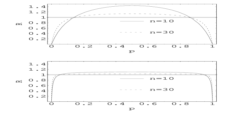
As shown in Figure 1, the MELE is always more efficient over most of the range and the relative efficiency tends to $1$ as $n\rightarrow\infty$ .

It is interesting to compare the MELE with Bayes estimate under a Jeffrey’s prior. The Jeffrey’s prior for $p$ is (Box and Tiao, p.35), $\pi(p)=1/\sqrt{p(1-p)}$ . Combining with the likelihood we can use Mathematica to show that the resulting Bayes estimator is $\tilde{p}=(1+4X)/(2+4n)$ . From Figure 1, we see that the Bayes estimator with Jeffrey’s prior tends have smaller mean-square error over an even slightly larger range of $p$ than the MELEbut the gain in efficiency with the mele can be greater. As with the MELE, the relative efficiency tends to $1$ as $n\rightarrow\infty$ . Once again, using Mathematica we can show that $R(\tilde{p},\hat{p}|p)>1$ provided

p\in\left({\frac{1+5\,n-{\sqrt{1+9\,n+20\,{n^{2}}}}}{2\,\left(1+5\,n\right)}},{\frac{1+5\,n+{\sqrt{1+9\,n+20\,{n^{2}}}}}{2\,\left(1+5\,n\right)}}\right).

The PMC criterion given in eqn. 1.1 is not applicable in the case of the binomial since due to the discreteness there can be ties in the values of the estimators. Keating, Mason and Sen (1993, §3.4.1) and one of the referees have suggested the following modified version of Pitman’s measure of closeness,

{\rm PMC}\left[\bar{\theta},\hat{\theta}|\theta\right]=\Pr\left\{|\bar{\theta}-\theta|<|\hat{\theta}-\theta|\right\}+{1\over 2}\Pr\left\{|\bar{\theta}-\theta|=|\hat{\theta}-\theta|\right\}.

With this modification, PMC is transitive and reflexive.

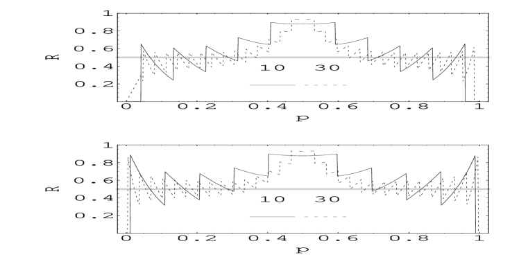
Figure 2 suggests the following asymptotic result,

\lim_{n\rightarrow\infty}{\rm PMC}(\bar{p},\hat{p}|p)=\left\{\begin{array}[]{ll}1&\mbox{$p=0.5$}\\ \frac{1}{2}&\mbox{$p\not=0.5,0,1$}\\ 0&\mbox{$p=0,1$}\end{array}\right.

(2.2)

This result may be established using the Geary-Rao Theorem (Keating, Mason and Sen, p.103).

Figure 2 also suggests that in terms of the PMC the advantage over the MLE of the MELE or of the Bayes estimate with a Jeffrey’s prior disappears when there is no prior information about $p$ .

3 Exponential Lifetimes

Consider a sample of size $n$ denoted by $X_{1},\ldots,X_{n}$ from an exponential distribution with mean $\mu$ and let $T=\sum_{i=1}^{n}X_{i}$ . The likelihood function for $\mu$ can be written $L(\mu)=\mu^{-n}e^{-T/\mu}$ , the MLE of $\mu$ is given by $\hat{\mu}=T/n$ and the MELE of $\mu$ is $\bar{\mu}=T/(n-2)$ . The Jeffrey’s prior for $\mu$ can be taken as $\mu^{-1}$ which produces a Bayesian estimate, $\tilde{\mu}=T/(n-1)$ .

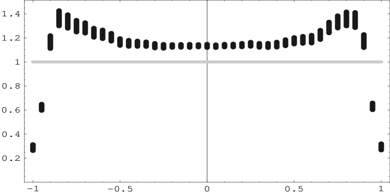
A simple computation with Mathematica gives the relative efficiency,

	$\displaystyle R(\bar{\mu},\hat{\mu})$	$\displaystyle=$	$\displaystyle{\frac{1}{n}}+{\frac{-5+n}{4+n}}$
		$\displaystyle=$	$\displaystyle 1-{\frac{8}{n}}+{\frac{36}{{n^{2}}}}-{\frac{144}{{n^{3}}}}+{\frac{576}{{n^{4}}}}-{\frac{2304}{{n^{5}}}}+{{{\mathcal{O}}({\frac{1}{n}})}^{6}}.$

Similarly, $R(\tilde{\mu},\hat{\mu})=1+1/n+4/(n+1)$ . Figure 3 shows that the MELE can be much less efficient.

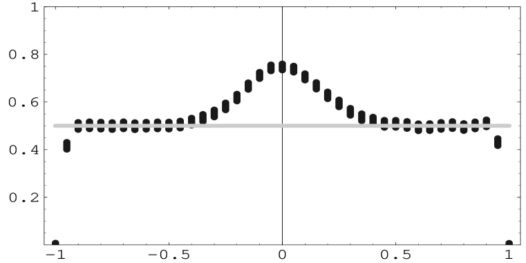
Since $T$ has a standard gamma distribution with shape parameter $n$ and scale parameter $\mu$ , the PMC is easily evaluated using the Geary-Rao Theorem (Keating, Mason and Sen, 1993, p.103). Letting $a=\bar{\mu}$ or $a=\tilde{\mu}$ , we can write

{\rm PMC}(a,\hat{\mu}|\mu)=\int_{0}^{b\mu}\frac{e^{-x/\mu}x^{n-1}\mu^{-n}}{\Gamma(n)}dx

where $b=n(n-2)/(n-1)$ or $b=2n(n-1)/(2n-1)$ according as $a=\bar{\mu}$ or $a=\tilde{\mu}$ . Notice that without loss of generality we may take $\mu=1$ since ${\rm PMC}(\bar{\mu},\hat{\mu}|\mu)={\rm PMC}(\bar{\mu},\hat{\mu}|1)$ . From Figure 4, ${\rm PMC}(a,\hat{\mu}|\mu)<0.5$ for both $a=\bar{\mu}$ or $a=\tilde{\mu}$ .

It is sometimes mistakenly thought that Theorem 4 or its Bayesian analogue guarantees that at least over some region of the parameter space, the MELE and the Bayes estimator will have outperform the MLE but this need not be the case.

4 MA(1) Process

4.1 Introduction

The MA(1) time series with mean $\mu$ may be written $Z_{t}=\mu+A_{t}+\theta A_{t-1}$ , where $Z_{t}$ denotes the observation at time $t=1,2,\ldots$ and $A_{t}$ , the innovation at time $t$ , is assumed to be a sequence of independent normal random variables with mean zero and variance $\sigma_{A}^{2}$ . The parameter $\theta$ determines the autocorrelation structure of the series and for identifiability we will assume that $|\theta|\leq 1$ . When $|\theta|<1$ , the model is invertible (Brockwell and Davis, 1991, §3.1). For simplicity we will examine the case where $\mu=0$ . Such MA(1) models often arise in practical applications as the model for a differenced nonstationary time series. The non-invertible case $\theta=1$ occurs when a series is over-differenced.

In large-samples, standard asymptotic theory suggests that the maximum likelihood estimate for $\theta$ , denoted by $\hat{\theta}$ , is approximately normal with mean $\theta$ and variance $(1-\theta^{2})/n$ where $n$ is the length of the observed time series. Cryer and Ledolter (1981) established the somewhat surprising result that $\Pr\{\hat{\theta}=\pm 1\}>0$ . This result holds for all finite $n$ and for all values of $\theta$ . For example when $n=50,\;\Pr\{\hat{\theta}=1|\theta=0\}=0.002$ and $\Pr\{\hat{\theta}=1|\theta=0.8\}=0.13$ (Cryer and Ledolter, 1981, Table 2). Let $\bar{\theta}$ denote the mean likelihood estimate of $\theta$ . In view of Theorem 1, this problem does not occur with $\bar{\theta}$ .

Now we will show that the MELE dominates the MLE both for the MSE and PMC criteria when $n=2$ . When $n=50$ , the MELE is better than the MLE unless the parameter $\theta$ is very close to $\pm 1$ . Since even the useless estimator obtained by ignoring the data and setting the estimate to $1$ does better when $\theta=1$ , we can conclude that MELE is generally a better estimator. Further mean-square error computations which support this conclusion for other values of $n$ are given by Quenneville (1993) and can be verified by the reader using the electronic supplement.

4.2 Exact Results for $n=2$

Given a Gaussian time series of length $2,Z_{1},Z_{2}$ , generated from the first-order moving average equation $Z_{t}=A_{t}-\theta A_{t-1}$ , where $A_{t}$ are independent normal random variables with mean zero and variance $\sigma_{A}^{2}$ . Let $W=-Z_{1}Z_{2}/(Z_{1}^{2}+Z_{2}^{2})$ . Then given data, $Z_{1},Z_{2}$ , the exact concentrated likelihood function for $\theta$ is (Cryer and Ledolter, 1981; Quenneville, 1993),

L(\theta|W)=\frac{\sqrt{1+\theta^{2}+\theta^{4}}}{1+\theta^{2}-2\theta W}

and

\hat{\theta}=\left\{\begin{array}[]{ll}-1&\mbox{$W\in[-0.5,-0.25]$}\\ \frac{1-\sqrt{1-16W^{2}}}{4W}&\mbox{$W\in(-0.25,0.25),W\not=0$}\\ 0&\mbox{$W=0$}\\ 1&\mbox{$W\in[0.25,0.5]$.}\end{array}\right.

Unfortunately $\bar{\theta}$ , cannot be evaluated symbolically. However using NIntegrate we can obtain it numerically. Numerical evaluation suggests that $\bar{\theta}$ is either a linear or close to a linear function of $W$ . To speed up our computations for the mean-square error of $\bar{\theta}$ , we use the FunctionInterpolation in Mathematica to construct $\bar{\theta}=\bar{\theta}(W)$ . The MSE and PMC for $\bar{\theta}$ and $\hat{\theta}$ are easily evaluated numerically using the pdf of $W,\;f_{W}(x)$ , derived by Quenneville (1993),

f_{W}(x)=\frac{2\sqrt{1+\theta^{2}+\theta^{4}}}{\pi\sqrt{1-4x^{2}}(1+\theta^{2}-2\theta x)},\;|x|\leq 1/2.

From Figures 5 and 6, it is seen that both the MELE and Bayesian estimator dominate the MLE both for the MSE and PMC criteria. The MELE is slightly better according to the MSE but according to the PMC the Bayes estimator is slightly better than the MELE.

4.3 Exact Symbolic Likelihood

Consider the MA(1) process defined by $Z_{t}=A_{t}-\theta A_{t-1}$ , where $A_{t}$ is assumed to be normal and independently distributed with mean zero and variance $\sigma_{A}^{2}$ . Given $n$ observations $Z^{\prime}=(Z_{1},\ldots,Z_{n})$ the exact log likelihood function of an ARMA process can be written (Newbold, 1974),

\log L(\theta,\sigma_{A}^{2})=-\frac{n}{2}\log(\sigma_{A}^{2})-\frac{1}{2}\log(D)-\frac{1}{2\sigma_{A}^{2}}S(\theta),

where $h^{\prime}=(1,\theta,\theta^{2},\ldots,\theta^{n}),\;D=h^{\prime}h$ and

S(\theta)=(Lz-hh^{\prime}Lz/D)^{\prime}(Lz-hh^{\prime}Lz/D),

where $L$ is the $(n+1)$ by $n$ matrix,

L=\left(\begin{array}[]{cccccc}0&0&0&\ldots&0&0\\ 1&0&0&\ldots&0&0\\ \theta&1&0&\ldots&0&0\\ \theta^{2}&\theta&1&\ldots&0&0\\ \vdots&\vdots&\vdots&\ldots&\vdots&\vdots\\ \theta^{n-2}&\theta^{n-3}&\theta^{n-4}&\ldots&1&0\\ \theta^{n-1}&\theta^{n-2}&\theta^{n-3}&\ldots&\theta&1\end{array}\right).

Maximizing over $\sigma_{A}^{2}$ the concentrated log likelihood is given by

\log L_{M}(\theta)=-\frac{n}{2}\log\left[S(\theta)/n\right]-\frac{1}{2}\log(D).

This expression for the concentrated loglikelihood is just as easy to write in Mathematica notation as it is in ordinary mathematical notation. Moreover, it can be evaluated symbolically or numerically.

LogLikelihoodMA1[t_, z_] :=
    Module[{n = Length[z], Lz, h, detma1, v, Sumsq},
      Lz = Join[{0},
          Table[Sum[z[[i]]] t^(j-i), {i, 1, j}], {j, 1, n}]];
      h = Table[t^j, {j, 0, Length[z]}];
      detma1 = h . h;
      v = -h . Lz/detma1;
      Sumsq = (Lz + h v). (Lz + h v);
      -n/2 Log[Sumsq/n /. t -> t] -
        1/2 Log[detma1 /. t -> t]
    ];

4.4 Efficient Numeric Likelihood Computations

Newbold’s algorithm can be made much more efficient when only numerical values of the log likelihood are needed by using the Mathematica Compiler and by re-writing the calculations involved to make more use of efficient Mathematica functions such as NestList, FoldList and Apply. First consider the computation of the vector $Lz$ which is of length $n+1$ . After some simplifications, we see that $Lz=(\alpha_{j})^{\prime}$ , where $\alpha_{0}=0$ is the first element and the remaining elements are defined recursively by $\alpha_{j}=\theta\alpha_{j-1}+Z_{j},\;j=1,2,\ldots,n$ , where $Z_{0}=0$ . This computation is efficiently performed by Mathematica’s FoldList. When we are just interested in numerical evaluation we use the compile function to generate native code which runs much faster.

GetLz=Compile[{{t,_Real},{z, _Real, 1}},
  FoldList[(#1 t + #2)&,0,z]];

The determinant, $D=1+\theta^{2}+\theta^{4}+\ldots+\theta^{2n}$ , is efficiently computed using NestList to generate the individual terms and then summing.

DetMA =Compile[{{t,_Real},{n, _Integer}},
  Apply[Plus,NestList[#1 t &,1,n]^2]];

Next, we evaluate the term $hLz/D$ . Since $hLz=\theta\alpha_{1}+\theta^{2}\alpha_{2}+\ldots+\theta^{n}\alpha_{n}$ we can use Horner’s Rule to efficiently compute this sum. Horner’s Rule is implemented in Mathematica using the function Fold.

Getu0 =Compile[{{t,_Real},{Lz, _Real, 1},{detma, _Real}},
       -Fold[#1 t + #2&,0,Reverse[Lz]]/detma];

The computation of the sum of squares function $S(\theta)=(Lz-hh^{\prime}Lz/D)^{\prime}(Lz-hh^{\prime}Lz/D)$ is straightforward. The Mathematica compiler can be used to optimize the vector computations.

GetSumSq =
  Compile[{{t,_Real},{Lz, _Real, 1},{u, _Real},{n, _Integer}},
    Apply[Plus,(Lz+NestList[#1 t &,1,n] u)^2]];

Finally, the concentrated loglikelihood function is defined. The computation speed is increased by about a factor of $50$ times when $n=50$ and is even larger for larger $n$ .

logLMA1F[t_, z_] :=
  Module[{n=Length[z]},
    Lz=GetLz[t,z];
    detma=DetMA[t,n];
    u=Getu0[t,Lz,detma];
    S=GetSumSq[t,Lz,u,n];
    -(1/2) Log[detma]- (n/2)Log[S/n]];

This function can be maximized using Mathematica’s nonlinear optimization function FindMinimum.

The mean likelihood estimate $\bar{\theta}$ can be evaluated using NIntegrate.

Meanle[z_]:=
  NIntegrate[t E^logLMA1F[t, z],{t,-1,1}]/
    NIntegrate[E^logLMA1F[t, z],{t,-1,1}]

Notice that in the above expression the loglikelihood function is evaluated separately in both the numerator and denominator. Hence, we can save function evaluations by using our own numerical quadrature routine.

SimpsonQuadratureWeights[k_,a_, b_]:=
  With[{h=(2 k)/3},
   {a+(b-a)Range[0,2 k]/(2k),
   Prepend[Append[Drop[Flatten[Table[{4,2},{k}]],{-1}],1],1]}]

{X,W}=SimpsonQuadratureWeights[100,-1,1];

GETMEANLEF=
  Compile[{{z, _Real, 1},
           {W, _Real, 1},{X, _Real, 1},{f, _Real, 1}},
           Plus@@(X f)/Plus@@f];ΨΨΨ
MEANLEF[z_]:=
  With[{f=Plus@@W E^(logLMA1F[#1,z]&/@X)},
    GETMEANLEF[z,W,X,f]];ΨΨΨΨΨ

Our tests indicate acceptable accuracy and about a $70\%$ improvement in speed as compared with Mathematica’s more sophisticated NIntegrate function.

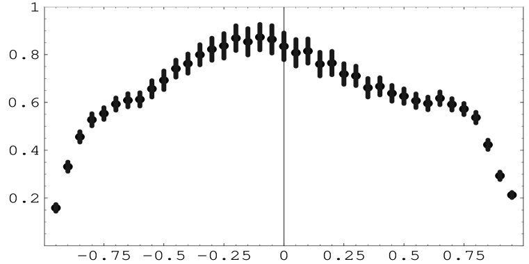
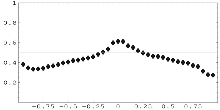
4.5 Simulation Results for $n=50$

Using the Mathematica algorithms for the MLE and MELE derived above, we determined $99.9\%$ confidence intervals for $R(\bar{\theta},\hat{\theta})$ and ${\rm PMC}(\bar{\theta},\hat{\theta})$ based on $10^{4}$ simulations for each of the $41$ parameter values $\theta=-1,-0.95,-0.90,\ldots,0.95,1$ . Figures 7 and 8 show that the MELE dominates except for the cases $\theta=\pm 1,\pm 0.95$ . We can safely conclude that the MELE is a better overall estimator than the MLE. Of course, as already pointed out another cogent reason for preferring the MELE to the MLE is that it does not produce noninvertible models.

If prior information is available then even better results can be obtained. Marriott and Newbold (1998) have developed an ingenious approach to the unit root problem in time series by noting this fact.

The simulations were repeated with the mean $\mu$ estimated by the sample average and there was no major change is results. The reader may like compare the estimators for other values of $n$ using the Mathematica functions available in the electronic supplement.

In the standard Bayesian analysis of the MA(1) model the prior is given by (Box and Jenkins, 1976, p. 250–258)

\pi(\theta)=1/\sqrt{1-\theta^{2}}.

The computations were repeated using this prior and as shown in Figures 9 and 10 the Bayes estimate with a Jeffrey’s prior performs about the same as the MELE.

5 Concluding Remarks

Previously Copas (1966) found that for AR(1) models, the MELE had lower MSE over much of the parameter region. Our results show that for the MA(1) the improvement is even somewhat better. The MSE is lower over a broader range and the piling-up effect on the MLE is avoided. Quenneville (1993) investigated the small sample properties of the MELE for many other time series models and gave a general algorithm for the MELE in ARMA models and found that in many cases the MELE produced estimates with smaller MSE over most of the parameter region. This work is further extended to state space prediction in Quenneville and Singh (1999).

We would also like to mention that in our opinion Mathematica provides an excellent and indeed unparalled environment for many types of fundamental mathematical statistical research. In comparison, no other computing environment provides such high quality capabilities simultaneously in: symbolics, numerics, graphics, typesetting and programming. The importance of a powerful user-oriented programming language for researchers is sometimes lacking in other environments. Stephan Wolfram once said that in his opinion the APL computing language had many good ideas in this direction and that Mathematica has incorporated all these capabilities and much more. A partial check on this is given in McLeod (1999) where it was found that most APL idioms could be more clearly expressed in Mathematica.

However, for applied statistics and data analysis, Splus may still be advantageous due to the wide usage by researchers and the high quality functions for advanced statistical methods that are available with Splus and in the associated infrastructure. From the educational viewpoint though this advantage may not be so important since many students and researchers like to understand the principles involved and with Mathematica it is as easy to write out the necessary functions in Mathematica notation as it would be to explain the procedures in a traditional mathematical notation.

6 References

1.

Andrews, D.F. (1997) Asymptotic expansions of moments and cumulants. Technical Report.
2.

Andrews, D.F. and Stafford, J.E. (1993) Tools for the symbolic computation of asymptotic expansions. Journal of the Royal Statistical Society, B 55, 613–627.
3.

Barnard, G.A., Jenkins, G.M. and Winsten, C.B. (1960) Likelihood inference and time series Journal of the Royal Statistical Society Series A 125, 321–372.
4.

Borowski, E.J. and Borwein, J.M. (1991) The HarperCollins Dictionary of Mathematics. New York: HarperCollins.
5.

Box, G.E.P. and Jenkins, G.M. (1976) Time Series Analysis: Forecasting and Control. San Francisco: Holden-Day.
6.

Box, G.E.P. and Tiao, G.C. (1973) Bayesian Inference in Statistical Analysis. Reading: Addison-Wesley.
7.

Brockwell, P.J. and Davis, R.A. (1991) Time Series Theory and Methods. New York: Springer-Verlag.
8.

Cabrera, J. F. (1989) Some experiments with maximum likelihood estimation using symbolic manipulations. Proceedings of the 21st Symposium on the Interface of Statistics and Computer Science, Edited by K. Berk.
9.

Copas, J. B. (1966) Monte Carlo results for estimation in a stable Markov time series. Journal of the Royal Statistical Society, A 129, 110–116.
10.

Cryer, J.D. and Ledolter, J. (1981) Small-sample properties of the maximum likelihood estimator in the first-order moving average model. Biometrika, 68, 691–694.
11.

Currie, I.D. (1995) Maximum likelihood estimation and Mathematica. it Applied Statistics, 44, 379–394.
12.

Dempster, A.P. (1998) Logicist statistics I. Models and modeling. Statistical Science 13, 248–276.
13.

Johnson, N.I. and Kotz, S. (1972) it Distributions in Statistics: Discrete Distributions. New York: Wiley.
14.

Keating, J.P., Mason, R.L. and Pranab, K.S. (1993) Pitman’s Measure of Closeness. Philadelphia: SIAM.
15.

Newbold, P. (1974) The exact likelihood function for a mixed autoregressive-moving average process. Biometrika, 61, 423–426.
16.

McLeod, A.I. (1999) APL-idioms in Mathematica. http://www.stats.uwo.ca/mcleod/epubs/idioms.
17.

McLeod, A.I. and Quenneville, B. (1999) Mathematica notebooks to accompany Mean likelihood estimation. http://www.stats.uwo.mcleod/epubs/mele.
18.

Marriott, J. and Newbold, P. (1998) Bayesian comparison of ARIMA and stationary ARMA models, International Statistical Review 66, 323–336.
19.

Pitman, E.J.G. (1937) The closest estimates of statistical parameters, Proceedings of the Cambridge Philosophical Society 33, 212–222. Biometrika 30, 391–421.
20.

Pitman, E.J.G. (1938) The estimation of the location and scale parameters of a continuous population of any given form, Biometrika 30, 391–421.
21.

Quenneville, B. (1993) Mean Likelihood Estimation and Time Series Analysis. Ph.D. Thesis, University of Western Ontario.
22.

Quenneville, B. and Singh, A.C. (1999) Bayesian prediction MSE for state space models with estimated parameters. Journal of Time Series Analysis (to appear).
23.

Ritov, Y. (1990) Asymptotic efficient estimators of the change point with unknown distributions. The Annals of Statistics 18, 1829–1839.
24.

Rubin, H. and Song, K.S. (1995) Exact computation of the asymptotic efficiency of the maximum likelihood estimators of a discontinuous signal in a Gaussian white noise. The Annals of Statistics 23, 732–739.
25.

Stafford, J.E. and Andrews, D.F. (1993) A symbolic algorithm for studying adjustments to the profile likelihood. Biometrika, 80, 715–730.
26.

Stafford, J.E., Andrews, D.F. and Wang, Y. (1994) Symbolic computation: a unified approach to studying likelihood. Statistics and Computing, 4, 235–245.
27.

Tanner, M.A. (1993) Tools for Statistical Inference. New York: Springer-Verlag.
28.

Wolfram, S. (1996) Mathematica. Champaign: Wolfram Research Inc.