Ly$\alpha$ Emitters with Very Large Ly$\alpha$ Equivalent Widths, EW₀(Ly$\alpha$) $\simeq 200-400$Å, at $z\sim 2$

Abstract

We present physical properties of spectroscopically confirmed Ly$\alpha$ emitters (LAEs) with very large rest-frame Ly$\alpha$ equivalent widths EW₀(Ly$\alpha$). Although the definition of large EW₀(Ly$\alpha$) LAEs is usually difficult due to limited statistical and systematic uncertainties, we identify six LAEs selected from $\sim 3000$ LAEs at $z\sim 2$ with reliable measurements of EW₀ (Ly$\alpha$) $\simeq 200-400$ Å given by careful continuum determinations with our deep photometric and spectroscopic data. These large EW₀(Ly$\alpha$) LAEs do not have signatures of AGN, but notably small stellar masses of $M_{\rm*}=10^{7-8}$ $M_{\rm\odot}$ and high specific star-formation rates (star formation rate per unit galaxy stellar mass) of $\sim 100$ Gyr^-1. These LAEs are characterized by the median values of $L({\rm Ly\alpha})=3.7\times 10^{42}$ erg s^-1 and $M_{\rm UV}=-18.0$ as well as the blue UV continuum slope of $\beta=-2.5\pm 0.2$ and the low dust extinction $E(B-V)_{\rm*}=0.02^{+0.04}_{-0.02}$, which indicate a high median Ly$\alpha$ escape fraction of $f_{\rm esc}^{\rm Ly\alpha}=0.68\pm 0.30$. This large $f_{\rm esc}^{\rm Ly\alpha}$ value is explained by the low Hi column density in the ISM that is consistent with FWHM of the Ly$\alpha$ line, ${\rm FWHM(Ly\alpha)}=212\pm 32$ km s^-1, significantly narrower than those of small EW₀(Ly$\alpha$) LAEs. Based on the stellar evolution models, our observational constraints of the large EW₀ (Ly$\alpha$), the small $\beta$, and the rest-frame Heii equivalent width imply that at least a half of our large EW₀(Ly$\alpha$) LAEs would have young stellar ages of $\lesssim 20$ Myr and very low metallicities of $Z<0.02Z_{\odot}$ regardless of the star-formation history.

1 INTRODUCTION

Photometric studies of Ly$\alpha$ emitters (LAEs: Cowie & Hu 1998; Rhoads et al. 2000; Ouchi et al. 2003; Malhotra & Rhoads 2004; Gronwall et al. 2007) have revealed that about $4-10\%$ ($10-40\%$) of LAEs at $z\sim 2-3$ ($z\sim 4-6$) show extremely large rest-frame Ly$\alpha$ equivalent widths, EW₀ (Ly$\alpha$) $\gtrsim 200$ Å ($z\sim 2-3$: Nilsson et al. 2007; Mawatari et al. 2012, $z\sim 4-6$: Malhotra & Rhoads 2002; Shimasaku et al. 2006; Ouchi et al. 2008; Zheng et al. 2014). Several spectroscopic studies have also identified LAEs with large EW₀ (Ly$\alpha$) values (Dawson et al. 2004; Wang et al. 2009; Adams et al. 2011; Kashikawa et al. 2012).

Schaerer (2003) and Raiter et al. (2010) have constructed stellar evolution models that cover various metallicities ($Z=0-1.0Z_{\rm\odot}$) and a wide range of initial mass functions (IMFs). According to the models of Schaerer (2003) and Raiter et al. (2010), the value of EW₀ (Ly$\alpha$) $\gtrsim 200$ Å can be explained by stellar populations with a very young stellar age ($\lesssim 10$ Myr), a very low metallicity, or a top-heavy IMF (cf., Charlot & Fall 1993; Malhotra & Rhoads 2002). Thus, large EW₀(Ly$\alpha$) LAEs are particularly interesting as candidates for galaxies at an early stage of the galaxy formation or galaxies with an exotic metallicity/IMF (Schaerer 2002). The models of Schaerer (2003) and Raiter et al. (2010) have shown that the Heii $\lambda 1640$ line is an useful indicator to break the degeneracy between the stellar age and metallicity. This is due to the fact that the high excitation level of Heii, $h\nu=54.4$ eV, can be achieved only by massive stars with extremely low metallicities ($Z\sim 0-5\times 10^{-6}$ $Z_{\rm\odot}$). These models predict that galaxies hosting zero-metallicity stars (Population III stars; hereafter Pop III) can emit Heii whose rest-frame EW, EW₀(Heii), is up to a few times 10 Å. The UV continuum slope ($\beta$), defined as $f_{\lambda}\propto\lambda^{\beta}$, is also powerful to place constraints on the stellar age and metallicity because the $\beta$ value ranges to as low as $\gtrsim-3.0$ depending on the stellar age and metallicity (Schaerer 2003; Raiter et al. 2010). Therefore, it is important to simultaneously examine EW₀(Ly$\alpha$), EW₀(HeII), and $\beta$ values to put constraints on stellar ages and metallicities of large EW₀(Ly$\alpha$) LAEs.

There are two problems in previous large EW₀(Ly$\alpha$) LAE studies. First, EW₀(Ly$\alpha$) measurements have large uncertainties. Because LAEs are generally faint in continua, it is difficult to measure the continuum flux at $1216$ Å from spectroscopic data. Thus, most LAE studies have estimated the continuum flux at $1216$ Å from photometric data in the wavelength range redward of $1216$ Å. Furthermore, previous studies have assumed the flat UV continuum slope, $\beta=-2.0$, to estimate the continuum flux at $1216$ Å. Since large EW₀(Ly$\alpha$) LAEs are typically very faint in the continuum (Ando et al. 2006), large uncertainties remain in EW₀(Ly$\alpha$) values even if the continuum fluxes at $1216$ Å are derived from photometric data. Second, detailed physical properties of large EW₀(Ly$\alpha$) LAEs have been scarcely investigated. There are no studies that placed constraints on stellar ages and metallicities of large EW₀(Ly$\alpha$) LAEs based on EW₀(Ly$\alpha$), EW₀(Heii), and $\beta$ values. Kashikawa et al. (2012) have examined the stellar age and metallicity of a large EW₀(Ly$\alpha$) LAE at $z\sim 6.5$ based on EW₀(Ly$\alpha$) and EW₀(Heii) values. However, the result is practically based on the EW₀(Ly$\alpha$) value because the EW₀(Heii) value is only an upper limit.

In this study, we examine physical properties of six large EW₀(Ly$\alpha$) LAEs that are spectroscopically confirmed at $z\sim 2$. By modeling deep FUV photometric data with no apriori assumption on $\beta$, we carefully estimate EW₀(Ly$\alpha$) and $\beta$ values of our LAEs. Remarkably, we find that our LAEs have large EW₀(Ly$\alpha$) values ranging from $160$ to $357$ Å with a mean value of $252\pm 30$ Å. The $\beta$ values of our LAEs vary from $1.6$ to $-2.9$ with a small median value of $-2.5\pm 0.2$. In order to place constraints on stellar ages and metallicities of our large EW₀(Ly$\alpha$) LAEs, we compare observational constraints of the large EW₀(Ly$\alpha$), the small $\beta$, and EW₀(Heii) with theoretical models of Schaerer (2003) and Raiter et al. (2010). Since these theoretical models have fine metallicity grids at the low metallicity range, we can investigate stellar ages and metallicities of our large EW₀(Ly$\alpha$) LAEs in detail. We also derive physical quantities such as the stellar mass ($M_{\rm*}$), the star formation rate (SFR), the full width at the half maximum, FWHM, of the Ly$\alpha$ lines, and the Ly$\alpha$ escape fraction ($f^{\rm Ly\alpha}_{\rm esc}$) from the spectral data and photometric data (SED fitting).

This paper is organized as follows. We describe our large EW₀(Ly$\alpha$) LAE sample and data in §2. In §3, we derive EW₀(Ly$\alpha$) and $\beta$ values as well as several observational quantities of our LAEs. A discussion in the context of physical properties of large EW₀(Ly$\alpha$) LAEs is given in §4, followed by conclusions in §5. Throughout this paper, magnitudes are given in the AB system (Oke & Gunn, 1983), and we assume a $\Lambda$CDM cosmology with $\Omega_{\small m}=0.3$, $\Omega_{\small\Lambda}=0.7$ and $H_{\small 0}=70$ km s^-1 Mpc^-1.

2 Sample and Data

2.1 Large EW₀(Ly$\alpha$) LAE Sample

Our large EW₀(Ly$\alpha$) LAEs are taken from the largest ($N\sim 3000$) parent LAE sample at $z\sim 2.2$ spanning in the COSMOS field, the Chandra Deep Field South (CDFS), and the Subaru/XMM-Newton Deep Survey (SXDS) (Nakajima et al. 2012, 2013; Konno et al. 2016; Kusakabe et al. in prep.). The parent sample is based on Subaru/Suprime-Cam imaging observations with our custom made narrow band filter, NB387. The central wavelength and the FWHM of NB387 are $3870$ Å and $94$ Å, respectively. The parent LAE sample has been selected by the following color criteria:

$$u^{*}-NB387>0.5\ \&\ B-NB387>0.2,$$ (1)

satisfying the condition that the EW₀(Ly$\alpha$) value should be larger than $30$ Å. The parent sample has been used to examine LAEs’ metal abundances and ionization parameters (Nakajima et al. 2012, 2013; Nakajima & Ouchi 2014), kinematics of the inter-stellar medium (ISM) (Hashimoto et al. 2013; Shibuya et al. 2014b; Hashimoto et al. 2015), diffuse Ly$\alpha$ haloes (Momose et al. 2014, 2016), morphologies (Shibuya et al. 2014a), dust properties (Kusakabe et al. 2015), and the Ly$\alpha$ luminosity function (Konno et al. 2016).

From the parent sample, we use six objects with strong NB387 excesses,

$$u^{*}-NB387>1.0\ \&\ B-NB387>1.4,$$ (2)

as well as Ly$\alpha$ identifications that are listed in Table 1: four from the COSMOS field, COSMOS-08501, COSMOS-40792, COSMOS-41547, and COSMOS-44993 and two from the SXDS-center (SXDS-C) field, SXDS-C-10535 and SXDS-C-16564. Since our targets are large EW₀(Ly$\alpha$) objects whose Ly$\alpha$ emission originates from star-forming activities, we examine if our sample includes a Ly$\alpha$ Blob (LAB: Møller & Warren 1998, Steidel et al. 2000). This is because Ly$\alpha$ emission of LABs is thought to be powered by AGN activities (e.g., Haiman & Rees 2001), superwinds from starburst galaxies (e.g., Taniguchi & Shioya 2000), and cold accretion (e.g., Haiman et al. 2000). To check the presence of LABs, we have inspected the isophotal areas of NB387 images that trace the Ly$\alpha$ morphologies. We have obtained $4.2$ arcsec² (COSMOS-08501), $1.1$ arcsec² (COSMOS-40792), $1.7$ arcsec² (COSMOS-41547), $1.5$ arcsec² (COSMOS-44993), $1.7$ arcsec² (SXDS-C-10535), and $6.2$ arcsec² (SXDS-C-16564). These isophotal areas correspond to the radii of $9-21$ kpc at $z\sim 2.2$. These radii are spatially compact compared to the half light radii of typical $z\sim 3$ LABs, $30-300$ kpc (Steidel et al. 2000; Matsuda et al. 2004). Thus, we conclude that our large EW₀(Ly$\alpha$) LAEs do not include a LAB.

Table 1: Sample of Large EW₀(Ly$\alpha$) LAEs

Object	$\alpha$(J2000)	$\delta$(J2000)	$u^{*}-NB387$	$B-NB387$	Line	$z_{\rm Ly\alpha}$	Sourcea
(1)	(2)	(3)	(4)	(5)	(6)	(7)	(8)
COSMOS-08501	10:01:16.80	+02:05:36.3	$1.45$	$2.17$	Ly$\alpha$ (MagE), H$\alpha$ (NIRSPEC)	$2.162$	N13, H15
COSMOS-40792	09:59:46.66	+02:24:34.2	$1.44$	$2.02$	Ly$\alpha$ (LRIS)	$2.209$	S14
COSMOS-41547	09:59:41.91	+02:25:00.0	$1.00$	$1.90$	Ly$\alpha$ (LRIS)	$2.152$	S14
COSMOS-44993	09:59:53.87	+02:27:11.0	$1.42$	$1.48$	Ly$\alpha$ (LRIS)	$2.214$	S14
SXDS-C-10535	02:17:41.92	-05:02:55.9	$1.11$	$1.42$	Ly$\alpha$ (LRIS)	$2.213$	S14
SXDS-C-16564	02:19:09:54	-04:57:13.3	$1.46$	$1.95$	Ly$\alpha$ (IMACS)	$2.176$	N12

(1) Object ID; (2) and (3) Right Ascension and Declination; (4) and (5) $u^{*}-NB387$ and $B-NB387$ colors; (6) Spectroscopically identified line(s) and instruments used for observations; (7) Redshifts inferred from the Ly$\alpha$ lines; and (8) Source of the information.

^a N12: Nakajima et al. (2012); N13: Nakajima et al. (2013); S14: Shibuya et al. (2014b); H15: Hashimoto et al. (2015).

2.2 Photometric Data

We performed photometry using SExtractor (Bertin & Arnouts 1996). We use $14$ bandpasses: $u^{*},NB387,B,V,r^{\prime},i^{\prime}$, and $z^{\prime}$ data taken with Subaru/Suprime-Cam, $J$ data taken with UKIRT/WFCAM, $H$ and $K$ data taken with CFHT/WIRCAM (UKIRT/WFCAM) for COSMOS (SXDS-C), and Spitzer/IRAC $3.6,4.5,5.8,$ and $8.0$ $\mu$m from the Spitzer legacy survey of the UDS fields.

For the detailed procedure of photometry, we refer the reader to Nakajima et al. (2012). Recently, Skelton et al. (2014) have re-calibrated zero-point magnitudes for the COSMOS and SXDS fields using 3D-HST (Brammer et al. 2012) and CANDELS (Grogin et al. 2011; Koekemoer et al. 2011) data. Skelton et al. (2014) have found that the zero-point magnitude offsets are from $0.00$ to $-0.25$. For secure estimates of physical quantities, we correct our zero-point magnitudes for the offsets listed in Tables $11$ and $12$ of Skelton et al. (2014). Table 2 summarizes the photometry of our objects.

Table 2: Photometry of our LAEs

Object	$u^{*}$	NB387	B	V	r’	i’	z’	J	H	Ks	[3.6]	[4.5]	[5.8]	[8.0]
COSMOS
08501	25.14	23.69	25.86	25.91	26.05	25.96	25.77	99.99	26.47	25.85	99.99	99.99	99.99	99.99
	(0.03)	(0.03)	(0.05)	(0.17)	(0.16)	(0.20)	(0.52)	(-)	(1.39)	(1.00)	(-)	(-)	(-)	(-)
40792	26.72	25.28	27.30	27.14	27.94	31.21	27.41	99.99	99.99	99.99	25.54	25.79	99.99	99.99
	(0.14)	(0.12)	(0.21)	(0.56)	(1.38)	(3.38)	(0.62)	(-)	(-)	(-)	(1.45)	(1.00)	(-)	(-)
41547	26.06	25.07	26.97	26.59	26.70	26.21	27.46	99.99	25.71	24.94	99.99	99.99	22.50	22.72
	(0.08)	(0.10)	(0.15)	(0.32)	(0.30)	(0.25)	(0.68)	(-)	(0.66)	(1.42)	(-)	(-)	(0.62)	(2.18)
44993	26.50	25.08	26.56	27.02	26.71	26.55	27.41	24.54	99.99	25.52	99.99	99.99	99.99	99.99
	(0.12)	(0.10)	(0.10)	(0.49)	(0.31)	(0.35)	(0.62)	(1.35)	(-)	(0.60)	(-)	(-)	(-)	(-)
offseta	-0.16	0.00	0.03	0.23	0.20	0.12	0.21	0.08	0.07	0.07	-0.02	0.03	0.05	0.12
SXDS-C
10535	25.84	24.73	26.15	26.29	26.64	26.61	26.94	27.12	27.54	25.64	25.92	99.99	99.99	99.99
	(0.08)	(0.10)	(0.08)	(0.12)	(0.22)	(0.22)	(0.83)	(0.62)	(1.78)	(0.72)	(1.45)	(-)	(-)	(-)
16564	24.14	22.68	24.63	24.83	24.97	25.09	25.16	25.18	23.83	24.40	25.49	29.91	99.99	99.99
	(0.02)	(0.01)	(0.02)	(0.03)	(0.05)	(0.05)	(0.14)	(0.37)	(0.19)	(0.20)	(1.11)	(4.24)	(-)	(-)
offseta	-0.25	0.00	0.03	0.06	0.18	0.25	0.18	-0.01	-0.06	-0.06	-0.05	0.00	-0.15	-0.15

All magnitudes are total magnitudes. $99.99$ mag indicates a negative flux density. Magnitudes in parentheses are $1\sigma$ uncertainties.

^a Zero-point magnitude offsets quoted from Skelton et al. (2014).

2.3 Spectroscopic Data

We carried out optical observations with Magellan/IMACS (PI: M. Ouchi), Magellan/MagE (PI: M. Rauch), and Keck/LRIS (PI: M. Ouchi). Details of the observations and data reduction procedures have been presented in Nakajima et al. (2012) (IMACS), Shibuya et al. (2014b) (LRIS), and Hashimoto et al. (2015) (MagE). The spectral resolutions for our observations were $R\sim 700$ (IMACS), $\sim 1100$ (LRIS), and $\sim 4100$ (MagE). SXDS-C-16564 was observed with IMACS, from which we identified the Ly$\alpha$ line (Nakajima et al. 2012). COSMOS-40792, COSMOS-41547, COSMOS-44933, and SXDS-C-10535 were observed with LRIS. Although these LAEs are as faint as $B\sim 26-27$, we detected the Ly$\alpha$ lines due to the high sensitivity of LRIS (Shibuya et al. 2014b). COSMOS-08501 was observed with MagE, from which we identified the Ly$\alpha$ line (Hashimoto et al. 2015). The H$\alpha$ line was also detected in COSMOS-08501 with Keck/NIRSPEC at the significance level of $\sim 5\sigma$ (Nakajima et al. 2013).

We additionally search for the Civ $\lambda 1549$ and Heii $\lambda 1640$ lines in our LAEs. We determine a line to be detected, if there exists an emission line above the $3\sigma$ sky noise around the wavelength expected from the Ly$\alpha$ redshift. In this analysis, we measure the sky noise from the spectrum within $50$ Å from the line wavelength. Neither Civ nor Heii was detected above $3\sigma$ in our LAEs. The flux upper limits of Civ are used to diagnose signatures of AGN in our LAEs (§2.4), while those of Heii enable us to place constraints on the stellar ages and metallicities of our LAEs (§4.3). Figure 1 shows 1D spectra corresponding to data around Ly$\alpha$, Civ, Heii, and H$\alpha$ lines.

Figure 1: From left to right, reduced 1D spectra corresponding to wavelength regions near Ly$\alpha$, Civ $\lambda 1549$, Heii $\lambda 1640$, and H$\alpha$ of our LAEs. The dashed lines in the 1D spectra show the expected locations of the lines.

2.4 AGN Activities in the Sample

We examine whether our LAEs host an AGN in three ways. First, we compare the sky coordinates of the objects with those in very deep archival X-ray and radio catalogs (Elvis et al. 2009). The sensitivity limits are $1.9\times 19^{-16}$ ($0.5-2.0$ keV band), $7.3\times 19^{-16}$ ($2-10$ keV band), and $5.7\times 19^{-16}$ erg ^-2 s^-1 ($0.5-10$ keV band). We also refer to the radio catalog constructed by Schinnerer et al. (2010). No counterpart for the LAEs is found in any of the catalogs.

Second, we search for the Civ $1549$ line whose high ionization potential can be achieved by AGN activities. The Civ line is not detected on an individual basis (§2.3). To obtain a strong constraint on the presence of an AGN, we stack the four LRIS spectra by shifting individual spectral data from the observed to the rest frame. We infer the systemic redshifts of the four LRIS objects as follows. The Ly$\alpha$ line is known to be redshifted with respect to the systemic redshift by $200-400$ km s^-1 (e.g., Steidel et al. 2010; Hashimoto et al. 2013; Shibuya et al. 2014b; Erb et al. 2014; Henry et al. 2015; Stark et al. 2015). Based on an anti-correlation between the Ly$\alpha$ velocity offset and EW₀(Ly$\alpha$) (Hashimoto et al. 2013; Shibuya et al. 2014b; Erb et al. 2014), we assume that our large EW₀(Ly$\alpha$) LAEs have the same Ly$\alpha$ velocity offsets as COSMOS-08501, $82\pm 40$ km s^-1 (Hashimoto et al. 2015). Figure 2 shows the stacked FUV spectrum of the four LRIS spectra. The Civ line is not detected even in the composite spectrum. We obtain the $3\sigma$ lower limit of the flux ratio, $f_{\rm Ly\alpha}$/$f_{\rm CIV}$ $>19.0$, where $f_{\rm Ly\alpha}$ and $f_{\rm CIV}$ are the Ly$\alpha$ and Civ fluxes, respectively. The flux ratio is significantly larger than that for $z\sim 2-3$ radio galaxies, $f_{\rm Ly\alpha}$/$f_{\rm CIV}$ $=6.9$ (Villar-Martín et al. 2007).

Finally, Nakajima et al. (2013) have examined the position of COSMOS-08501 in the BPT diagram (Baldwin et al. 1981). As shown in Figure $3$ of Nakajima et al. (2013), the upper limit of the flux ratio of [Nii] $\lambda 6584$ and H$\alpha$, log([Nii] $\lambda 6584$/H$\alpha$) $\lesssim-0.7$, indicates that COSMOS-08501 does not host an AGN.

Thus, we conclude that no AGN activity is seen in our LAEs.

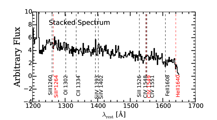
Figure 2: Composite rest-frame UV spectrum of the four LRIS spectra. The black and red vertical dashed lines indicate wavelengths of interstellar absorption lines and emission lines, respectively.

3 Results

3.1 SED Fitting

We perform stellar population synthesis model fitting to our LAEs to derive the stellar mass ($M_{\rm*}$), stellar dust extinction ($E(B-V)_{\rm*}$), the stellar age, and the star-formation rate (SFR). For the detailed procedure, we refer the reader to Ono et al. (2010a, b). Briefly, we use the stellar population synthesis model of GALAXEV (Bruzual & Charlot, 2003) including nebular emission (Schaerer & de Barros, 2009), and adopt the Salpeter IMF (Salpeter, 1955). For simplicity, we use constant star formation models. Indeed, several authors have assumed the constant star-formation history (SFH) for LAE studies at $z\sim 2$ (e.g., Kusakabe et al. 2015; Hagen et al. 2016) and at $z>3$ (see Table 6 in Ono et al. 2010b). Because LAEs are metal poor star-forming galaxies (Finkelstein et al. 2011; Nakajima et al. 2012, 2013; Song et al. 2014), we choose a metallicity of $Z=0.2$ $Z_{\odot}$. We use Calzetti’s law (Calzetti et al., 2000) for $E(B-V)_{\rm*}$, and apply $18\%$ IGM attenuation of continuum photons shortward of Ly$\alpha$ using the prescription of Madau (1995). To derive the best-fit parameters, we use all bandpasses mentioned in §2.2 except for ${\it u^{*}}$ and NB387-band data. Neither ${\it u^{*}}$ nor NB387-band data have been used since the photometry of these bands is contaminated by IGM absorption and/or Ly$\alpha$ emission. Figure 3 shows the best-fit model spectra with the observed flux densities. The derived quantities and their $1\sigma$ uncertainties are summarized in Table 3.

In Table 3, our LAEs have stellar masses mostly $M_{\rm*}=10^{7-8}M_{\rm\odot}$ with a median value of $7.1^{+4.8}_{-2.8}\times 10^{7}M_{\rm\odot}$. The median value is smaller than that of $z\sim 2$ LAEs with small EW₀(Ly$\alpha$), $2-5\times 10^{8}M_{\rm\odot}$ (Nakajima et al. 2012; Hagen et al. 2016). Nilsson et al. (2011); Oteo et al. (2015) and Shimakawa et al. (2016) have also studied stellar masses of $z\sim 2$ LAEs. In these studies, there are no LAEs with $M_{\rm*}<10^{8}M_{\rm\odot}$. These results indicate that our sample is consisted of low-mass LAEs.

The dust extinction of our LAEs varies from $E(B-V)_{\rm*}=0.00$ to $0.25$ with a median value of $0.02^{+0.04}_{-0.02}$. This is lower than the typical dust extinction of $z\sim 2$ LAEs, $E(B-V)_{\rm*}\sim 0.2-0.3$ (Guaita et al. 2011; Nakajima et al. 2012; Oteo et al. 2015). This result shows that our LAEs have small amounts of dust.

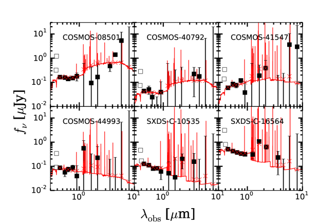
Figure 3: Results of SED fitting for our LAEs. The filled squares denote the photometry points used for SED fitting, while the open squares are those omitted in SED fitting due to the contamination of Ly$\alpha$ emission and IGM absorption. The red lines present the best-fit model spectra, while the red crosses correspond to the flux densities at individual passbands expected from the best-fit models.

Table 3: Results of SED fitting

Object	$\chi^{2}$	log($M_{*}$)	$E(B-V)_{\rm*}$	log(age)	log(SFR)
		($M_{\odot}$)		(yr)	($M_{\odot}$/yr)
(1)	(2)	(3)	(4)	(5)	(6)
COSMOS-8501	1.8	$7.8^{+1.2}_{-0.3}$	$0.08^{+0.04}_{-0.08}$	$6.2^{+2.8}_{-1.1}$	$1.68^{+1.24}_{-1.44}$
COSMOS-40792	3.8	$8.9^{+0.2}_{-2.1}$	$0.00^{+0.10}_{-0.00}$	$9.4^{+0.0}_{-4.4}$	$-0.37^{+2.53}_{-0.00}$
COSMOS-41547	4.8	$8.1^{+0.4}_{-0.3}$	$0.25^{+0.04}_{-0.07}$	$6.9^{+0.8}_{-0.4}$	$1.27^{+0.42}_{-0.51}$
COSMOS-44993	3.1	$7.6^{+1.2}_{-0.5}$	$0.03^{+0.09}_{-0.03}$	$7.4^{+1.6}_{-2.3}$	$0.23^{+2.28}_{-0.28}$
SXDS1-10535	3.4	$7.3^{+0.5}_{-0.0}$	$0.00^{+0.02}_{-0.00}$	$6.5^{+1.2}_{-1.4}$	$0.80^{+1.50}_{-0.59}$
SXDS1-16564	9.2	$7.9^{+0.0}_{-0.0}$	$0.00^{+0.00}_{-0.00}$	$6.5^{+0.1}_{-0.1}$	$1.43^{+0.1}_{-0.1}$

Stellar metallicity is fixed to 0.2 $Z_{\odot}$.

(1) Object ID; (2) $\chi^{2}$ of the fitting; (3) Stellar mass; (4) Stellar dust extinction; (5) Stellar age; and (6) Star-formation rate.

3.2 Careful Estimates of EW₀(Ly$\alpha$) and $\beta$

We model a realistic FUV spectrum of a LAE to derive EW₀(Ly$\alpha$), the Ly$\alpha$ luminosity ($L({\rm Ly\alpha})$), the UV absolute magnitude ($M_{\rm UV}$), and $\beta$. As mentioned in §1, EW₀(Ly$\alpha$) estimates in previous studies are based on several assumptions: (i) the UV continuum slope is flat, $\beta=-2.0$, and (ii) the pass-bands are ideal top-hat response functions (e.g., Malhotra & Rhoads 2002; Guaita et al. 2011; Mawatari et al. 2012). These factors add systematic uncertainties in EW₀(Ly$\alpha$).

In this work, the LAE spectrum is modeled as a combination of a delta-function Ly$\alpha$ line and a linear continuum,

$$f_{\rm\nu,Ly\alpha}=F({\rm Ly\alpha})\times\delta(\nu-\nu_{\rm Ly\alpha}),$$ (3)

$$f_{\rm\nu,cont}=A\times\nu^{-(\beta_{\rm 1200-2800}+2)},$$ (4)

where $f_{\rm\nu,Ly\alpha}$ ($f_{\rm\nu,cont}$ ) is the Ly$\alpha$ (continuum) flux per unit frequency in erg cm^-2 s^-1 Hz^-1, while $F({\rm Ly\alpha})$ is the integrated flux of the line in erg cm^-2 s^-1. The function $\delta(\nu-\nu_{\rm Ly\alpha})$ is a delta-function, and the function $A$ corresponds to the amplitude of the continuum flux. In equation (4), $A$ is expressed as

$$A=(2.0\times 10^{15})^{\beta_{\rm 1200-2800}+2}\times 10^{-0.4(m_{\rm 1500}+48.6)},$$ (5)

where $\beta_{\rm 1200-2800}$ is the UV continuum slope in the rest-frame wavelength range of $1200-2800$ Å, while $m_{1500}$ indicates the apparent magnitude at 1500 Å. With $f_{\rm\nu,cont}$ and $F({\rm Ly\alpha})$ in equations (3) and (4), the modeled flux in the $i$th band is defined as

$$f_{\rm\nu,model}^{(i)}=\frac{\int f_{\rm\nu}T_{\rm\nu}^{(i)}d\nu}{\int T_{\rm\nu}^{(i)}d\nu}=$$ (6)

$$\frac{\int_{\nu_{\rm s}}^{\nu_{\rm Ly\alpha}}f_{\rm\nu,cont}T_{\rm\nu}^{(i)}d\nu+F({\rm Ly\alpha})T_{\rm\nu,Ly\alpha}^{(i)}+\alpha\int_{\nu_{\rm Ly\alpha}}^{\nu_{\rm e}}f_{\rm\nu,cont}T_{\rm\nu}^{(i)}d\nu}{\int_{\nu_{\rm s}}^{\nu_{\rm e}}T_{\rm\nu}^{(i)}d\nu}.$$ (7)

In equation (7), $T_{\nu}^{(i)}$ is the response curve of the $i$th band. The constants of $\nu_{\rm s}$ and $\nu_{\rm e}$ indicate the frequencies corresponding to the upper and lower ends of the response curves, respectively. The constant $T_{\nu,Ly\alpha}^{(i)}$ is the response curve value of the $i$th band at the Ly$\alpha$ frequency, $\nu_{\rm Ly\alpha}$, where $\nu_{\rm Ly\alpha}$ is calculated from the Ly$\alpha$ redshift, $z_{\rm Ly\alpha}$ (Table 1). Finally, $\alpha$ means the continuum photon transmission shortward of Ly$\alpha$ after the IGM absorption. Using the prescription of Madau (1995), at $z\simeq 2$, it is

$$\alpha=\begin{cases}0.82&(\nu\geq\nu_{\rm Ly\alpha})\\ 1.0&(\nu<\nu_{\rm Ly\alpha}).\end{cases}$$

To estimate EW₀(Ly$\alpha$) and other quantities, we compare the modeled flux in the $i$th band with the observed one in the $i$th band. The observed flux in the $i$th band is expressed as

$$f_{\rm\nu,obs}^{(i)}=10^{-0.4({\rm AB^{(i)}}+48.6)},$$ (8)

where ${\rm AB^{(i)}}$ is the AB magnitude of the $i$th band listed in Table 2. For each LAE, we use six rest-frame FUV data, from ${\it u^{*}}$ to $i^{\prime}$-band. With equations (7) and (8), we search for the best-fitting spectrum that minimizes

$$\chi^{2}=\sum_{i}^{6}\frac{\bigl{\{}f^{(i)}_{\rm\nu,obs}-f^{(i)}_{\rm\nu,model}\bigl{[}F(Ly\alpha),\beta_{\rm 1200-2800},m_{\rm 1500}\bigr{]}\bigr{\}}^{2}}{\sigma^{2}\bigl{[}f^{(i)}_{\rm\nu,obs}\bigr{]}},$$ (9)

where $\sigma\bigl{[}f^{(i)}_{\rm\nu,obs}\bigr{]}$ is the photometric and systematic errors in the $i$th bandpass. The uncertainties in the best-fit parameters correspond to the $1\sigma$ confidence interval, $\Delta\chi^{2}<1.0$. With best-fit parameters of $\beta_{\rm 1200-2800}$ and $m_{\rm 1500}$, we obtain $f_{\rm\nu,cont}$ from equations (4) and (5). The flux $f_{\rm\nu,cont}$ is then converted into $f_{\rm\lambda,cont}$ from the relation

$$f_{\rm\lambda,cont}=\frac{c}{\lambda^{2}}\times f_{\rm\nu,cont},$$ (10)

where $c$ is the speed of light. Using equation (10), we derive the continuum flux at 1216 Å, $f_{\rm cont,1216}$, to obtain EW₀(Ly$\alpha$) as

$${\rm EW_{\rm 0}(Ly\alpha)}=\frac{F(Ly\alpha)}{f_{\rm cont,1216}}\times\frac{1}{1+z_{\rm Ly\alpha}}.$$ (11)

We obtain $M_{\rm UV}$ from the continuum flux at 1500 Å, $f_{\rm cont,1500}$, as below:

$$M_{\rm UV}=m_{1500}-5{\rm log}(d_{L}/{\rm 10pc})+2.5{\rm log}(1+z_{\rm Ly\alpha}),$$ (12)

where $d_{L}$ indicates the luminosity distance corresponding to $z_{\rm Ly\alpha}$.

Figure 4 shows the best-fit model spectra. As can be seen, our technique reproduces the rest-frame UV SEDs. The best-fit parameters and their $1\sigma$ uncertainties are summarized in Table 4. In Table 4, we find that our LAEs have large EW₀(Ly$\alpha$) values ranging from $160$ to $357$ Å with a mean value of $252\pm 30$ Å. We confirm that LAEs with EW₀(Ly$\alpha$) $\gtrsim 200$ Å exist by our fitting method with no apriori assumption on UV continuum slopes. UV continuum slopes vary from $\beta_{\rm 1200-2800}=-1.6$ to $-2.9$ with small mean and median values of $-2.3\pm 0.2$ and $-2.5\pm 0.2$, respectively. The median Ly$\alpha$ luminosity of our LAEs is $L({\rm Ly\alpha})=3.7^{+2.8}_{-2.8}\times 10^{42}$ erg s^-1. This is broadly consistent with the characteristic Ly$\alpha$ luminosity of $z\sim 2$ LAEs obtained by Hayes et al. (2010); Ciardullo et al. (2012) and Konno et al. (2016). The median UV absolute magnitude of our LAEs is $M_{\rm UV}=-18.5$. Figure 5 plots $\beta$ against ${M_{\rm UV}}$ for our LAEs and Lyman-break galaxies (LBGs) at $z\sim 2$ (Bouwens et al. 2009; Hathi et al. 2013; Alavi et al. 2014). We note that the error bar of the data points of Bouwens et al. (2009) indicate the $1\sigma$ of the $\beta$ distribution at each magnitude bin. In Figure 5, our LAEs have $\beta$ values comparable to or smaller than the LBGs at a given ${M_{\rm UV}}$ value, implying large EW₀(Ly$\alpha$) objects have small UV continuum slopes. This trend is consistent with previous results (e.g., Stark et al. 2010; Hathi et al. 2016).

In §4.3, we constrain the stellar ages and metallicities of our LAEs based on comparisons of the EW₀(Ly$\alpha$) and UV continuum slopes with stellar evolution models of Schaerer (2003) and Raiter et al. (2010). Although we have estimated UV continuum slopes at the wavelength range of $1200-2800$ Å, Schaerer (2003) and Raiter et al. (2010) have computed UV continuum slopes at the wavelength range of $1800-2200$ Å. Thus, we also calculate UV continuum slopes of our LAEs at the same wavelength range, $\beta_{\rm obs.1800-2200}$, with the following equation:

$$\beta_{\rm obs.1800-2200}=-\frac{V-(r^{\prime}+i^{\prime})/2}{\rm 2.5log(\lambda_{\it V}/(\lambda_{\it r^{\prime}}+\lambda_{\it i^{\prime}})/2)}-2,$$ (13)

where $V$, $r^{\prime}$, and $i^{\prime}$ are the magnitudes listed in Table 2, while $\lambda_{V}$, $\lambda_{r^{\prime}}$, and $\lambda_{i^{\prime}}$ correspond to the central wavelengths of each band, $5500$, $6300$, and $7700$ Å, respectively. We obtain $\beta_{\rm obs.1800-2200}$ $=-2.0\pm 0.1$ (COSMOS-08501), $-3.3\pm 4.0$ (COSMOS-40792), $-1.9\pm 0.1$ (COSMOS-41547), $-1.7\pm 0.2$ (COSMOS-44993), $-2.3\pm 0.1$ (SXDS-C-10535), and $-2.2\pm 0.1$ (SXDS-C-16564). Figure 6 plots $\beta_{\rm 1200-2800}$ against $\beta_{\rm obs.1800-2200}$. The data points lie on the one-to-one relation, showing that the two UV continuum slopes are consistent with each other.

We note here that the models of Schaerer (2003) and Raiter et al. (2010) do not take into account dust extinction effects on UV continuum slopes. For fair comparisons, we derive the intrinsic UV continuum slopes, $\beta_{\rm 1800-2200}$. We find that UV continuum slopes increase by 0.5 for $E(B-V)_{\rm*}=0.1$ based on a combination of the empirical relation, $A_{\rm 1600}=4.43+1.99\beta$ (Meurer et al. 1999), and Calzetti extinction, $A_{\rm 1600}=k_{\rm 1600}E(B-V)_{\rm*}$ ($k_{\rm 1600}=10$; Ouchi et al. 2004). With $E(B-V)_{\rm*}$ in Table 3, we obtain $\beta_{\rm 1800-2200}=-2.4^{+0.2}_{-0.4}$ (COSMOS-08501), $-3.3^{+7.9}_{-7.9}$ (COSMOS-40792), $-3.1^{+0.3}_{-0.4}$ (COSMOS-41547), $-1.9^{+0.6}_{-0.4}$ (COSMOS-44993), $-2.3^{+0.1}_{-0.1}$ (SXDS-C-10535), and $-2.2^{+0.1}_{-0.1}$ (SXDS-C-16564). In this calculation, we have adopted $2\sigma$ errors in $\beta_{\rm obs.1800-2200}$ to obtain conservative uncertainties in $\beta_{\rm 1800-2200}$. The mean and median correction factors are as small as $-0.3\pm 0.2$ and $-0.1\pm 0.2$, respectively. This is due to the fact that our LAEs have the low median stellar dust extinction value, $E(B-V)_{\rm*}=0.02^{+0.04}_{-0.02}$. One might be concerned about the systematic uncertainty of using two different models; we have adopted the model of GALAXEV to derive stellar dust extinction and the correction factors for UV continuum slopes, whereas we use the models of Schaerer (2003) and Raiter et al. (2010) to compare with $\beta_{\rm 1800-2200}$. However, the systematic uncertainty is negligibly small because our LAEs have small $\beta_{\rm obs.1800-2200}$ values. Our conservative uncertainties in $\beta_{\rm 1800-2200}$ would include these systematic errors.

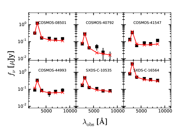
Figure 4: Rest-frame UV SEDs, from ${\it u^{*}}$ to $i^{\prime}$-band data, of our LAEs. The filled squares denote the photometry used for the fits, while the red crosses correspond to the flux densities at individual passbands expected from the best-fit models.

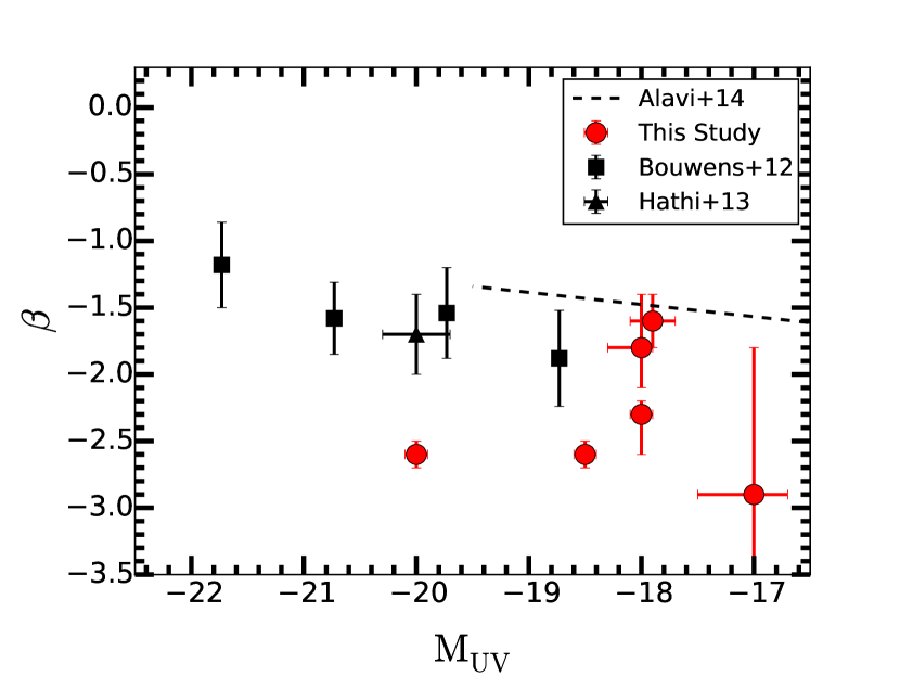
Figure 5: UV spectral slope ($\beta$) as a function of the absolute UV magnitude at $1500$Å ($M_{\rm UV}$) at $z\sim 2$. The red circles are our LAEs, where we adopt $\beta_{\rm 1200-2800}$ as the $\beta$ values. The dashed line is the best linear fit for $z\sim 2$ lensed LBGs (Alavi et al., 2014), while the black triangle is the average value of $z\sim 2$ LBGs (Hathi et al., 2013). The black squares indicate $z\sim 2$ LBGs studied by Bouwens et al. (2009), where error bars denote the $1\sigma$ of the distribution at each magnitude bin.

Figure 6: Comparison of the two UV continuum slopes, $\beta_{\rm 1200-2800}$ and $\beta_{\rm obs.1800-2200}$, for our LAEs. The dashed line indicates the one-to-one relation.

Table 4: Results of Careful Estimates of EW₀(Ly$\alpha$) and $\beta$

Object	$\chi^{2}$	EW0(Ly$\alpha$)	$L({\rm Ly\alpha})$	$M_{\rm UV}$	$\beta_{\rm 1200-2800}$
		(Å)	(1042 erg s-1)
(1)	(2)	(3)	(4)	(5)	(6)
COSMOS-8501	8.5	$284^{+39}_{-16}$	$8.9^{+0.8}_{-0.5}$	$-18.0^{+0.1}_{-0.1}$	$-2.3^{+0.3}_{-0.1}$
COSMOS-40792	2.3	$357^{+96}_{-114}$	$2.5^{+0.3}_{-0.4}$	$-17.0^{+0.5}_{-0.3}$	$-2.9^{+1.0}_{-1.1}$
COSMOS-41547	13.5	$303^{+59}_{-46}$	$3.3^{+0.3}_{-0.4}$	$-17.9^{+0.2}_{-0.2}$	$-1.6^{+0.2}_{-0.2}$
COSMOS-44993	2.3	$215^{+115}_{-22}$	$2.9^{+0.8}_{-0.4}$	$-18.0^{+0.3}_{-0.1}$	$-1.8^{+0.3}_{-0.4}$
SXDS-C-10535	5.8	$160^{+12}_{-16}$	$4.1^{+0.4}_{-0.8}$	$-18.5^{+0.1}_{-0.1}$	$-2.6^{+0.1}_{-0.1}$
SXDS-C-16564	18.7	$195^{+7}_{-8}$	$20.0^{+1.2}_{-1.5}$	$-20.0^{+0.1}_{-0.1}$	$-2.6^{+0.1}_{-0.1}$

(1) Object ID; (2) $\chi^{2}$ of the fitting; (3) and (4) Rest-frame Ly$\alpha$ EW and Ly$\alpha$ luminosity; (5) UV absolute magnitude; and (6) UV spectral slope at the rest-frame wavelength range of $1800-2200$ Å.

3.3 FWHM of Ly$\alpha$ Lines

One of the advantages of our LAEs is that they have Ly$\alpha$ detections. We examine the FWHM of the Ly$\alpha$ line, FWHM(Ly$\alpha$). To derive FWHM(Ly$\alpha$) values, we apply a Monte Carlo technique exactly the same way as is adopted in Hashimoto et al. (2015). Briefly, we measure the $1\sigma$ noise in the Ly$\alpha$ spectrum set by the continuum level at wavelengths longer than $1216$ Å. Then we create $10^{3}$ fake spectra by perturbing the flux at each wavelength of the true spectrum by the measured $1\sigma$ error. For each fake spectrum, the wavelength range that encompasses half the maximum flux is adopted as the FWHM. We adopt the median and standard deviation of the distribution of measurements as the median and error values, respectively. The measurements corrected for the instrumental resolutions, FWHM_int(Ly$\alpha$), are listed in the column 2 of Table 5. We do not obtain the FWHM_int(Ly$\alpha$) of SXDS-C-16564 because its spectral resolution of the Ly$\alpha$ line, $R=600$, is insufficient for a reliable measurement. Hereafter, we eliminate SXDS-C-16564 from the sample when we discuss the FWHM_int(Ly$\alpha$) of our LAEs. FWHM_int(Ly$\alpha$) values range from 118 to 310 km s^-1 with a mean value of $212\pm 32$ km s^-1.

For comparisons, we also measure FWHM_int(Ly$\alpha$) values of nine $z\sim 2$ LAEs with small EW₀(Ly$\alpha$) values in the literature (Hashimoto et al. 2013; Nakajima et al. 2013; Shibuya et al. 2014b; Hashimoto et al. 2015). Among the LAEs studied in these studies, we do not use COSMOS-30679 whose Ly$\alpha$ emission is contaminated by a cosmic ray (Hashimoto et al. 2013). Hereafter, we refer this sample as “small EW₀(Ly$\alpha$) LAEs”. The mean EW₀(Ly$\alpha$) is $65\pm 10$ Å, while the mean FWHM_int(Ly$\alpha$) is calculated to be $389\pm 51$ km s^-1. Table 6 summarizes the EW₀(Ly$\alpha$) and FWHM_int(Ly$\alpha$) values of the small EW₀(Ly$\alpha$) LAEs. In addition, Trainor et al. (2015) have also investigated Ly$\alpha$ profiles of LAEs at $z\sim 2.7$. For the composite spectrum of 32 LAEs that have both Ly$\alpha$ and nebular line detections, the typical EW₀(Ly$\alpha$) value is $44$ Å, while the mean FWHM_int(Ly$\alpha$) value is $309\pm 22$ km s^-1. Using a sample of the large EW₀(Ly$\alpha$) LAEs, the small EW₀(Ly$\alpha$) LAEs, and the LAEs and LBGs in Trainor et al. (2015), we plot EW₀(Ly$\alpha$) as a function of FWHM_int(Ly$\alpha$) in Figure 7. In this figure, the data points of Trainor et al. (2015) cover the small EW₀(Ly$\alpha$) range complementary to our LAE results. We carry out the Spearman rank correlation test to evaluate the significance of a correlation. The rank correlation coefficient is $\rho=-0.72$, while the probability satisfying the null hypothesis is $P=0.002$. The result indicates that FWHM_int(Ly$\alpha$) anti-correlates with EW₀(Ly$\alpha$). We also carry out the Spearman rank correlation test for objects with similar $M_{\rm UV}$ values. For six LAEs satisfying $-20\leqq M_{\rm UV}\leqq-18$ (open circles in Figure 7), we obtain $\rho=-0.94$ and $P=0.016$. The result confirms that the anti-correlation is not due to the selection effect in $M_{\rm UV}$. Although Tapken et al. (2007) have claimed a qualitatively similar anti-correlation between EW₀(Ly$\alpha$) and FWHM_int(Ly$\alpha$) for their small EW₀(Ly$\alpha$) LAEs at a high-$z$ range of $z\sim 2.7-4.5$, no correlation test has been carried out. In our study, we have identified for the first time the anti-correlation based on a statistical test. Moreover, we have found the anti-correlation at the range of EW₀(Ly$\alpha$) $\gtrsim 200$ Å.

Several other studies have also studied FWHM_int(Ly$\alpha$) values of LAEs at a high-$z$ range of $z\sim 3-7$. Tapken et al. (2007) have investigated EW₀(Ly$\alpha$) and FWHM_int(Ly$\alpha$) values of individual LAEs at $z\sim 2.7-4.5$. In this study, the mean EW₀(Ly$\alpha$) is $47\pm 13$ Å, while the mean FWHM_int(Ly$\alpha$) is $472\pm 53$ km s^-1. These values are consistent with those of the small EW₀(Ly$\alpha$) LAEs (Table 6). At $z=5.7$ and $6.6$, Ouchi et al. (2010) have measured FWHM_int(Ly$\alpha$) values of composite spectra of LAEs. The sample of Ouchi et al. (2010) do not include large EW₀(Ly$\alpha$) LAEs. Nevertheless, the mean FWHM_int(Ly$\alpha$) values are $265\pm 37$ km s^-1 and $270\pm 16$ km s^-1 for $z=5.7$ and $6.6$, respectively, smaller than those of the small EW₀(Ly$\alpha$) LAEs (Table 6). This would be due to strong Ly$\alpha$ scattering in the IGM at $z\sim 6-7$ compared to that at $z\sim 2$: the IGM scattering significantly narrows the blue part of Ly$\alpha$ profile at $z\sim 6-7$ (Laursen et al. 2011).

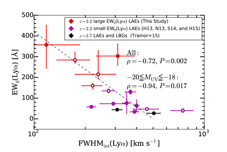
Figure 7: FWHM(Ly$\alpha$) corrected for the instrumental resolution, FWHM_int(Ly$\alpha$), plotted against EW₀(Ly$\alpha$). Note that the x-axis is in the log-scale. The red circles are our large EW₀(Ly$\alpha$) LAEs at $z\sim 2.2$, while the magenta circles indicate the small EW₀(Ly$\alpha$) LAEs at $z\sim 2.2$ (Hashimoto et al., 2013; Nakajima et al., 2013; Shibuya et al., 2014b; Hashimoto et al., 2015). The two black circles show the results for composite spectra of 32 LAEs and 65 LBGs at $z\sim 2.7$ (Trainor et al., 2015). For the whole sample, the Spearman rank correlation coefficient for the relation is $\rho=-0.72$, while the probability satisfying the null hypothesis is $P=0.002$. The dashed line is the linear fit to the data points. The six open circles indicate the LAEs with similar $M_{\rm UV}$ values, $-20\leqq M_{\rm UV}\leqq-18$, respectively. For the six LAEs, the Spearman rank correlation test gives $\rho=-0.94$ and $P=0.017$.

Table 5: Summary of Spectroscopic Properties of our Large EW₀(Ly$\alpha$) LAEs

Object	FWHMint(Ly$\alpha$)	$3\sigma$ $f_{\rm He{\sc II}}/f_{\rm Ly\alpha}$	3$\sigma$ EW0(HeII)
	(km s-1)	(Å)
(1)	(2)	(3)	(4)
COSMOS-08501	$174\pm 38$	$-$	$-$
COSMOS-40792	$118\pm 68$	$0.11^{+0.01}_{-0.02}$	$91^{+38}_{-27}$
COSMOS-41547	$310\pm 78$	$0.10^{+0.01}_{-0.01}$	$40^{+4}_{-3}$
COSMOS-44993	$238\pm 64$	$0.12^{+0.03}_{-0.02}$	$41^{+5}_{-4}$
SXDS1-10535	$221\pm 30$	$0.08^{+0.01}_{-0.02}$	$18^{+2}_{-2}$
SXDS1-16564	$-$	$0.02^{+0.01}_{-0.01}$	$7^{+2}_{-2}$

The symbol g- h indicates we have no measurement. (1) Object ID; (2) FWHMs of the Ly$\alpha$ lines corrected for the instrumental resolutions; (3) 3$\sigma$ upper limits of the flux ratio of Heii and Ly$\alpha$; and (4) 3$\sigma$ upper limits of the rest-frame Heii EW.

Table 6: Properties of small EW₀(Ly$\alpha$) LAEs

Object	EW0(Ly$\alpha$)	FWHMint(Ly$\alpha$)	Sourcea
	(Å)	(km s-1)
(1)	(2)	(3)	(4)
CDFS-3865	$64\pm 29$	$400\pm 15$	H13, N13, H15
CDFS-6482	$76\pm 52$	$350\pm 20$	H13, N13, H15
COSMOS-13636	$73\pm 5$	$292\pm 49$	H13, N13, H15
COSMOS-43982b	$130\pm 12$	$368\pm 26$	H13, N13, H15
COSMOS-08357	$47\pm 8$	$460\pm 79$	S14, H15
COSMOS-12805	$34\pm 6$	$389\pm 23$	S14, H15
COSMOS-13138	$40\pm 10$	$748\pm 114$	S14, H15
SXDS-10600	$58\pm 3$	$217\pm 13$	S14, H15
SXDS-10942	$135\pm 10$	$274\pm 23$	S14, H15

(1) Object ID; (2) Rest-frame Ly$\alpha$ EWs; (3) FWHMs of the Ly$\alpha$ lines corrected for the instrumental resolutions; and (4) Source of the information

^a H13: Hashimoto et al. (2013); N13: Nakajima et al. (2013); S14: Shibuya et al. (2014b); H15: Hashimoto et al. (2015)

^b AGN-like object

3.4 Upper Limits on the Flux Ratio of Heii/Ly$\alpha$ and EW₀(Heii)

We derive $3\sigma$ upper limits of the flux ratio, $f_{\rm HeII}$/$f_{\rm Ly\alpha}$, where $f_{\rm HeII}$ and $f_{\rm Ly\alpha}$ are the Heii and Ly$\alpha$ fluxes, respectively. We do not derive the flux ratio for COSMOS-08501 whose FUV data have been obtained with MagE. This is because the flux calibration of echelle spectra is often inaccurate (Willmarth & Barnes 1994). Following the procedure in Kashikawa et al. (2012), we obtain the $3\sigma$ upper limits of the Heii fluxes. These Heii fluxes are given from the wavelength ranges of 8.8 (4.8) Å for the IMACS (LRIS) spectra under the assumptions that the Heii lines are not resolved. The derived $3\sigma$ upper limits are $f_{\rm HeII}$/$f_{\rm Ly\alpha}=0.11^{+0.01}_{-0.02}$ (COSMOS-40792), $0.10^{+0.01}_{-0.01}$ (COSMOS-41547), $0.12^{+0.03}_{-0.02}$ (COSMOS-44993), $0.08^{+0.01}_{-0.02}$ (SXDS-C-10535), and $0.02^{+0.01}_{-0.01}$ (SXDS-C-16564) (the column 3 of Table 5). These $3\sigma$ upper limits are stronger than the $2\sigma$ upper limit of $f_{\rm HeII}$/$f_{\rm Ly\alpha}=0.23$ derived for a strong LAE at $z=6.3$ (Nagao et al. 2005). Moreover, these $3\sigma$ upper limits are comparable to the $3\sigma$ upper limits of $f_{\rm HeII}$/$f_{\rm Ly\alpha}\sim 0.02-0.06$ obtained for LAEs at $z\sim 3.1-3.7$ (Ouchi et al. 2008) and at $z=6.5$ (Kashikawa et al. 2012). Recently, Sobral et al. (2015) have reported the Heii line detection from a strong LAE at $z=6.6$, CR7, at the significance level of $6\sigma$. In this study, the rest-frame EW, EW₀(Heii), is measured to be $\sim 80$ Å (see also Bowler et al. 2016 who have obtained EW₀(Heii) $=40\pm 30$ Å with deep near-infrared photometric data). The measured flux ratio of CR7 is $f_{\rm HeII}$/$f_{\rm Ly\alpha}=0.23\pm 0.10$.

We calculate the fraction of large EW₀(Ly$\alpha$) LAEs with Heii detections among large EW₀(Ly$\alpha$) LAEs, combining our results with those in the literature. There are nine LAEs that satisfy EW₀(Ly$\alpha$) $\gtrsim$ 130 Å. These LAEs include five, one, one, and two objects from this study, Nagao et al. (2005), Kashikawa et al. (2012), and Sobral et al. (2015), respectively. We thus estimate the fraction to be $\sim$ $10\%$ (1/9).

We also examine $3\sigma$ upper limits of the EW₀(Heii). To do so, we derive the continuum flux at 1640 Å from photometric data with fitting results (§3.2). These estimates give us $3\sigma$ limits of EW₀(Heii) $\leqq$ $91^{+38}_{-27}$ Å (COSMOS-40792), $40^{+4}_{-3}$ Å (COSMOS-41547), $41^{+5}_{-4}$ Å (COSMOS-44993), $18^{+2}_{-2}$ Å (SXDS-C-10535), and $7^{+2}_{-2}$ Å (SXDS-C-16564) (the column 4 of Table 5). We use the $3\sigma$ upper limits of the EW₀(Heii) to place constraints on the stellar ages and metallicities of our LAEs (§4.3).

3.5 Coarse Estimates of the Ly$\alpha$ Escape Fraction

The Ly$\alpha$ escape fraction, $f^{\rm Ly\alpha}_{\rm esc}$, is defined as the ratio of the observed Ly$\alpha$ flux to the intrinsic Ly$\alpha$ flux produced in a galaxy. This quantity is mainly determined by a neutral hydrogen column density, $N_{\rm HI}$, or a dust content in the ISM. If the ISM has a low $N_{\rm HI}$ value or a low dust content, a high $f^{\rm Ly\alpha}_{\rm esc}$ value is expected because Ly$\alpha$ photons are less scattered and absorbed by dust grains (e.g., Atek et al. 2009; Hayes et al. 2011; Cassata et al. 2015)

Many previous studies have estimated Ly$\alpha$ escape fractions on the assumptions of Case B, the Salpeter IMF, and the Calzetti’s dust extinction law. These assumptions would increase systematic uncertainties in the estimates of the Ly$\alpha$ escape fractions. Nevertheless, in order to compare Ly$\alpha$ escape fractions of our LAEs with those in the literature, we obtain Ly$\alpha$ escape fractions conventionally as

$$f^{\rm Ly\alpha}_{\rm esc}=\frac{L_{\rm obs}({\rm Ly}\alpha)}{L_{\rm int}({\rm Ly}\alpha)},$$ (14)

where subscripts “int” and “obs” refer to intrinsic and observed quantities, respectively. We infer $L_{\rm int}({\rm Ly}\alpha)$ from the SFRs in Table 3 using $L_{\rm int}({\rm Ly}\alpha)$ [erg s^-1] $=1.1\times 10^{42}$ SFR [$M_{\rm\odot}$ yr^-1] (Kennicutt 1998) on the assumption of Case B. For COSMOS-08501 that has the H$\alpha$ detection, we quote the $f^{\rm Ly\alpha}_{\rm esc}$ value estimated from the extinction-corrected H$\alpha$ luminosities calculated by Nakajima et al. (2013). We have obtained $f^{\rm Ly\alpha}_{\rm esc}$ = $1.21^{+0.31}_{-0.38}$ (COSMOS-08501), $5.33^{+2045}_{-0.91}$ (COSMOS-40792), $0.16^{+0.26}_{-0.11}$ (COSMOS-41547), $1.55^{+294}_{-0.85}$ (COSMOS-44993), $0.59^{+18}_{-0.45}$ (SXDS-C-10535), and $0.68^{+0.04}_{-0.05}$ (SXDS-C-16564). For the three objects that have relatively small errors, COSMOS-08501, COSMOS-41547, and SXDS-C-16564, the mean and median Ly$\alpha$ escape fractions are $f^{\rm Ly\alpha}_{\rm esc}=0.68\pm 0.30$ and $0.68\pm 0.30$, respectively. These values are much higher than the average Ly$\alpha$ escape fraction of $z\sim 2$ galaxies, $f^{\rm Ly\alpha}_{\rm esc}$ $\sim 2-5\%$ (Hayes et al. 2010; Steidel et al. 2011; Ciardullo et al. 2014; Oteo et al. 2015; Matthee et al. 2016), and even higher than the average value of $z\sim 2$ LAEs, $f^{\rm Ly\alpha}_{\rm esc}$ $\sim 10-37\%$ (Steidel et al. 2011; Nakajima et al. 2012; Kusakabe et al. 2015; Trainor et al. 2015; Erb et al. 2016).

Figure 8 plots $f^{\rm Ly\alpha}_{\rm esc}$ against $E(B-V)_{*}$, $\beta$, and $M_{\rm*}$. We also plot the data points of $z\sim 2$ LAEs studies by Song et al. (2014) and Oteo et al. (2015) with both Ly$\alpha$ and H$\alpha$ detections. In these studies, Ly$\alpha$ escape fractions have been estimated with H$\alpha$ luminosities. Although no individual measurements of UV continuum slopes are given in Song et al. (2014), we calculate $\beta_{\rm 1800-2200}$ values of the LAEs with equation (13) using the $V,r,$ and $i-$band photometry listed in Table 3 of Song et al. (2014). For the consistency, we adopt $\beta_{\rm 1800-2200}$ for our LAEs. Oteo et al. (2015) have shown that $f^{\rm Ly\alpha}_{\rm esc}$ anti-correlates with $E(B-V)_{*}$, $\beta$, and $M_{\rm*}$. The result of Oteo et al. (2015) indicates that Ly$\alpha$ photons preferentially escape from low-mass and low dust content galaxies. With the median values of $E(B-V)_{*}$ = $0.02^{+0.04}_{-0.02}$, $\beta_{1800-2200}$ = $-2.2\pm 0.2$, and $M_{\rm*}$ = $7.9^{+4.6}_{-2.9}\times 10^{7}$ $M_{\rm\odot}$, our LAEs can be regarded as the extreme cases in these trends.

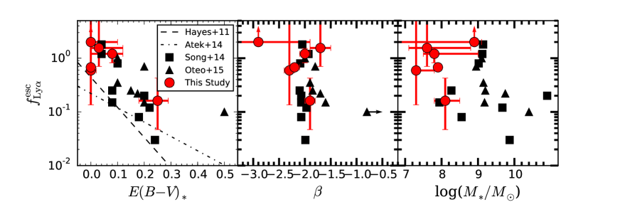
Figure 8: $f^{\rm Ly\alpha}_{\rm esc}$ plotted against $E(B-V)_{\rm*}$, $\beta$, and $M_{\rm*}$. The red circles denote our LAEs. The black squares are nine LAEs at $z\sim 2$ with Ly$\alpha$ and H$\alpha$ detections (Song et al., 2014), whereas the black triangles show seven LAEs at $z\sim 2$ with Ly$\alpha$ and H$\alpha$ (Oteo et al., 2015). In the left panel, the dashed and dot-dashed lines indicate the relation between $f^{\rm Ly\alpha}_{\rm esc}$ and $E(B-V)_{\rm*}$ for $z\sim 0-1$ (Atek et al., 2014) and $z\sim 2-3$ galaxies (Hayes et al., 2011), respectively. In the middle panel, we adopt $\beta_{\rm 1800-2200}$ for our LAEs.

4 Discussion

4.1 Mode of Star Formation

There is a relatively tight relation between SFRs and stellar masses of galaxies called the star formation main sequence (SFMS) (e.g., Daddi et al. 2007; Rodighiero et al. 2011; Speagle et al. 2014). Galaxies lie on the SFMS are thought to be in a long-term constant star-formation mode, while those lie above the SFMS are forming stars in a rapid starburst mode (Rodighiero et al. 2011). We note here that the star-formation mode is different from the SFH (see §3.1). As explained, star-formation mode refers to the position of a galaxy in the relation between SFRs and stellar masses. In contrast, SFHs express the functional forms of SFRs, e.g., $e^{-t/\tau}$ for the exponentially declining SFH, where $t$ and $\tau$ indicate the age and the typical timescale, respectively. The burst SFH indicates the declining SFH with $\tau<100$ Myr (e.g., Hathi et al. 2016). In the case of the constant SFH, the SFR is constant over time. With these in mind, we investigate the mode of star-formation of our LAEs with SFRs and stellar masses in §3.1.

Figure 9 plots SFRs against stellar masses for our LAEs. Figure 9 also includes the data points of LAEs in the literature (Kusakabe et al. 2015; Taniguchi et al. 2015; Hagen et al. 2016), BzK galaxies (Rodighiero et al. 2011), and optical emission line galaxies (Hagen et al. 2016) at $z\sim 2-3$. For COSMOS-08501, we also plot its SFR estimated from the extinction-corrected H$\alpha$ luminosities calculated by Nakajima et al. (2013). In Figure 9, the median of the six large EW₀(Ly$\alpha$) LAEs is shown as the red star. The median data point indicates that our LAEs are typically lie above the lower-mass extrapolation of the $z\sim 2$ SFMS (Daddi et al. 2007; Speagle et al. 2014). The specific SFRs (sSFR $\equiv$ SFR/$M_{\rm*}$) of our LAEs are mostly in the range of sSFR $=10-1000$ Gyr^-1 with a median value of $\sim 100$ Gyr^-1. The median sSFR of our LAEs is higher than those of LAEs and oELGs at $z\sim 2$ in Hagen et al. (2016), $\sim 10$ Gyr^-1.

Before interpreting the result, we note that stellar masses and SFRs in this study are derived from SED fitting on the assumption of the constant SFH. Thus, we need to check if our LAEs have high sSFRs on the assumption of other SFHs. Schaerer, de Barros, & Sklias (2013) have examined how physical quantities depend on the choice of SFHs. This study includes exponentially declining, exponentially rising, and constant SFHs. As can be seen from Figures 4 and 7 in Schaerer, de Barros, & Sklias (2013), stellar masses (SFRs) are the largest (smallest) for the constant SFH case among the various SFH cases. This means that the true sSFRs of our LAEs could be larger than what we have obtained. Therefore, our LAEs have high sSFRs regardless of the choice of SFHs.

A straightforward interpretation of the offset toward the high sSFR is that our large EW₀(Ly$\alpha$) LAEs are in the burst star-formation mode. As discussed in detail by Hagen et al. (2016), the offset can be also due to (i) a possible change in the slope of the SFMS at the low-mass range, (ii) errors in the estimates of SFRs and stellar masses, or due to (iii) the selection bias against objects with high sSFRs at the low-mass range. As to the second point, Kusakabe et al. (2015) have shown that typical LAEs favor the Small Magellanic Cloud (SMC) attenuation curve (Pettini et al. 1998) rather than the Calzetti’s curve (Calzetti et al. 2000). Kusakabe et al. (2015) have demonstrated that SFRs are roughly ten times overestimated if one uses the Calzetti’s curve (blue symbols in Figure 9). However, we stress that our estimates of SFRs and stellar masses remain unchanged regardless of the extinction curve because our LAEs have small UV continuum slopes. Therefore, the second scenario is unlikely for our LAEs. As to the third point, Shimakawa et al. (2016) have investigated SFRs and stellar masses of LAEs with $M_{\rm*}>10^{8}M_{\rm\odot}$ at $z\sim 2.5$. In contrast to our results and those in Hagen et al. (2016), LAEs in Shimakawa et al. (2016) follow the SFMS. Thus, it is possible that the high sSFRs of our LAEs are simply due to the selection bias. A large and uniform sample of galaxies with $M_{\rm*}=10^{7-8}$ is needed for a definitive conclusion.

Recently, Taniguchi et al. (2015) have reported six rare LAEs at $z\sim 3$ that have large EW₀(Ly$\alpha$) values and evolved stellar populations. Their EW₀(Ly$\alpha$) values range from $107$ to 306 Å with a mean value of $188\pm 30$ Å. Taniguchi et al. (2015) have found that these LAEs lie below the SFMS, suggesting that these LAEs are ceasing star forming activities. Based on the fact that our LAEs and those in Taniguchi et al. (2015) have similar EW₀(Ly$\alpha$) values, the EW₀(Ly$\alpha$) value is not necessarily a good indicator of the mode of star-formation.

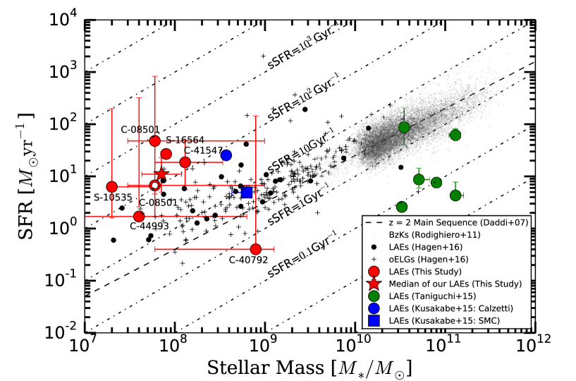
Figure 9: SFRs plotted against $M_{\rm*}$ for our large EW₀(Ly$\alpha$) LAEs and objects at $z\sim 2-3$ in the literature, where dot-dashed lines represent specific SFRs (sSFR $\equiv$ SFR/$M_{\rm*}$). The red filled circles show our six large EW₀(Ly$\alpha$) LAEs with a median stellar mass of $M_{\rm*}=7.1^{+4.8}_{-2.8}\times 10^{7}M_{\odot}$. The red open circle is COSMOS-08501 whose SFR estimated from the extinction-corrected H$\alpha$ luminosities (Nakajima et al. 2013). The red star means the median of the six LAEs. The gray dots indicate $z\sim 2$ BzK galaxies (Rodighiero et al., 2011), while the dashed line shows the SFMS at z = 2 (Daddi et al., 2007). The black circles and crosses are luminous (L(Ly$\alpha$)$>10^{43}$ erg s^-1) LAEs and optical emission line (e.g., [Oii], H$\beta$, and [Oiii]) galaxies (oELGs) at $z\sim 2$ studied by Hagen et al. (2016), respectively. The green circles indicate $z\sim 3$ LAEs with large EW₀(Ly$\alpha$) values and evolved stellar populations (Taniguchi et al., 2015). The blue circle and square denote the results of the stacking of 214 $z\sim 2$ LAEs on the assumption of the Calzetti’s curve and the SMC attenuation curve, respectively (Kusakabe et al., 2015).

4.2 Interpretations of the Small FWHM_int(Ly$\alpha$) in Large EW₀(Ly$\alpha$) LAEs

In Figure 7, we have demonstrated that there is an anti-correlation between EW₀(Ly$\alpha$) and FWHM_int(Ly$\alpha$). In this relation, our large EW₀(Ly$\alpha$) LAEs have small FWHM_int(Ly$\alpha$) values. We give three interpretations of the small FWHM_int(Ly$\alpha$) in our LAEs .

First, assuming uniform expanding shell models, Verhamme et al. (2015) have theoretically shown that the small FWHM_int(Ly$\alpha$) value is expected in the case of a low $N_{\rm HI}$ value in the ISM (see Figure 1 of Verhamme et al. 2015). If the physical picture of the theoretical study is true, the small FWHM_int(Ly$\alpha$) of our large EW₀(Ly$\alpha$) LAEs suggest that our LAEs would have low $N_{\rm HI}$ values in the ISM.

Second, Gronke & Dijkstra (2016) have performed Ly$\alpha$ radiative transfer calculations of multiphase ISM models. The result shows that narrow Ly$\alpha$ profiles can be reproduced by two cases, one of which is on the condition that a galaxy has a low covering fraction of the neutral gas . Thus, our large EW₀(Ly$\alpha$) LAEs may have lower covering fractions of the neutral gas than small EW₀(Ly$\alpha$) objects. Indeed, based on the analysis of the EW of low-ionization metal absorption lines, several studies have observationally shown that the neutral-gas covering fraction is low for galaxies with strong Ly$\alpha$ emission (e.g., Jones et al. 2013; Shibuya et al. 2014b; Trainor et al. 2015)

Finally, on the assumption that the FWHM_int(Ly$\alpha$) value is determined by a dynamical mass to the first order, the small FWHM_int(Ly$\alpha$) values of our large EW₀(Ly$\alpha$) LAEs imply that our LAEs would have low dynamical masses compared to small EW₀(Ly$\alpha$) objects. Although we admit that the FWHM_int(Ly$\alpha$) value is dominantly determined by radiative transfer effects rather than dynamical masses, there is an observational result that may support this interpretation. Hashimoto et al. (2015) and Trainor et al. (2015) have found that EW₀(Ly$\alpha$) anti-correlates with the FWHM value of nebular emission lines (e.g., H$\alpha$, [Oiii]), FWHM(neb). Since the FWHM(neb) value should correlate with the dynamical mass (e.g., Erb et al. 2006, 2014), the anti-correlation between EW₀(Ly$\alpha$) and FWHM(neb) means that large EW₀(Ly$\alpha$) LAEs have low dynamical masses. Among the large EW₀(Ly$\alpha$) LAEs, COSMOS-8501 has the H$\alpha$ detection. However, only an upper limit of the FWHM of the H$\alpha$ line is derived because the line is not resolved (FWHM(neb) $<200$ km s^-1; Hashimoto et al. 2015). This prevents us from obtaining a definitive conclusion on which of the three interpretations are likely for our LAEs.

4.3 Constraints on Stellar Ages and Metallicities

We place constraints on the stellar ages and metallicities of our LAEs by comparisons of our observational constrains of $\beta$, EW₀(Heii), and EW₀(Ly$\alpha$) with the stellar evolution models of Schaerer (2003) and Raiter et al. (2010).

4.3.1 Stellar Evolutionary Models

Schaerer (2003) and the extended work of Raiter et al. (2010) have constructed stellar evolution models that cover various stellar metallicities ($Z=0-1.0$ $Z_{\rm\odot}$), a variety of IMFs, and two star-formation histories of the instantaneous burst (burst SFH) and constant star-formation (constant SFH). These studies have theoretically examined the evolutions of spectral properties including emission lines for the stellar ages from 10⁴ yr to 1 Gyr. From the theoretical computations, these studies have provided evolutions of $\beta$, EW₀(Heii), and EW₀(Ly$\alpha$). To compute theoretical values of EW₀(Ly$\alpha$) and EW₀(Heii), Schaerer (2003) and Raiter et al. (2010) have assumed Case B recombination. One of the advantages of the models of Schaerer (2003) and Raiter et al. (2010) is that the models have fine metallicity grids at an extremely low metallicity range. These fine metallicity grids are useful because large EW₀(Ly$\alpha$) LAEs are thought to have extremely low metallicities. Among the results of Schaerer (2003) and Raiter et al. (2010), we use the predictions for six metallicities, $Z=0$ (Pop III), $5\times 10^{-6}$ $Z_{\odot}$, $5\times 10^{-4}$ $Z_{\odot}$, $0.02$ $Z_{\odot}$, $0.2$ $Z_{\odot}$, and $1.0$ $Z_{\odot}$. We adopt three power-law IMFs, (A) the Salpeter IMF at the mass range of $1-100$ $M_{\odot}$, (B) the top-heavy Salpeter IMF at the mass range of $1-500$ $M_{\odot}$, and (C) the Scalo IMF (Scalo 1986) at the mass range of $1-100$ $M_{\odot}$. Table 7 summarizes the IMFs and their parameters.

Figure 10 plots the evolutions of $\beta$, EW₀(Heii), and EW₀(Ly$\alpha$). The top panels of Figue 10 are the $\beta$ evolutions. $\beta$ values are sensitive to the stellar and nebular continuum. The $\beta$ evolution for extremely low metallicity cases ($Z=0-5\times 10^{-4}$ $Z_{\odot}$) is significantly different from that for relatively high metallicity cases ($Z=0.002-1.0$ $Z_{\odot}$). We explain the burst SFH case. In the relatively high metallicity cases ($Z=0.002-1.0$ $Z_{\odot}$), the $\beta$ value monotonically increases as the stellar age increases. This is due to the fact that the dominant stellar continuum is red for old stellar ages. The value of $\beta\sim-2.7$ is expected at the very young stellar age of log(age yr^-1) $\sim 6.0-7.0$. In contrast, in the extremely low metallicity cases ($Z=0-5\times 10^{-4}$ $Z_{\odot}$), the $\beta$ value behaves as a two-value function. This is because the $\beta$ value is determined by both the stellar and nebular continuum at the extremely low metallicities cases. In these cases, the nebular continuum is very red for young stellar ages. Thus,at the very young stellar age of log(age yr^-1) $\sim 6.0-6.5$, the $\beta$ value is relatively large, $\beta\sim-2.3$, due to the balance between the red nebular continuum and the blue stellar continuum. The contribution of the red nebular continuum to the $\beta$ value becomes negligible at log(age yr^-1) $\gtrsim 7.0$ because of the rapid decrease of ionizing photons. Therefore, the $\beta$ value reaches down to $\beta\sim-3.0$ at log(age yr^-1) $\sim 7.0-7.5$, then monotonically increases. For the constant SFH, the evolution of $\beta$ is smaller than that of the burst SFH.

The second top panels of Figure 10 show the EW₀(Heii) evolutions. The EW₀(Heii) value rapidly decreases as the metallicity increases: EW₀(Heii) $>5$ Å is expected only for $Z<5\times 10^{-6}$ $Z_{\rm\odot}$. In the case of the burst SFH, the timescale for the Heii line to be visible is short, log(age yr^-1) $\lesssim 7.0$. This timescale reflects the lifetime of extremely massive hot stars. Again, the evolution of EW₀(Heii) is larger in the burst SFH than that of the constant SFH.

The bottom panels of Figure 10 indicate the evolution of EW₀(Ly$\alpha$). A high EW₀(Ly$\alpha$) value is expected for a young stellar age and a low metallicity. In the case of the burst SFH, the timescale for the Ly$\alpha$ line to be visible is log(age yr^-1) $\lesssim 7.5$. This reflects the lifetime of O-type stars. The maximum EW₀(Ly$\alpha$) value can reach EW₀(Ly$\alpha$) $\sim 800-1500$ Å for the Pop III metallicity.

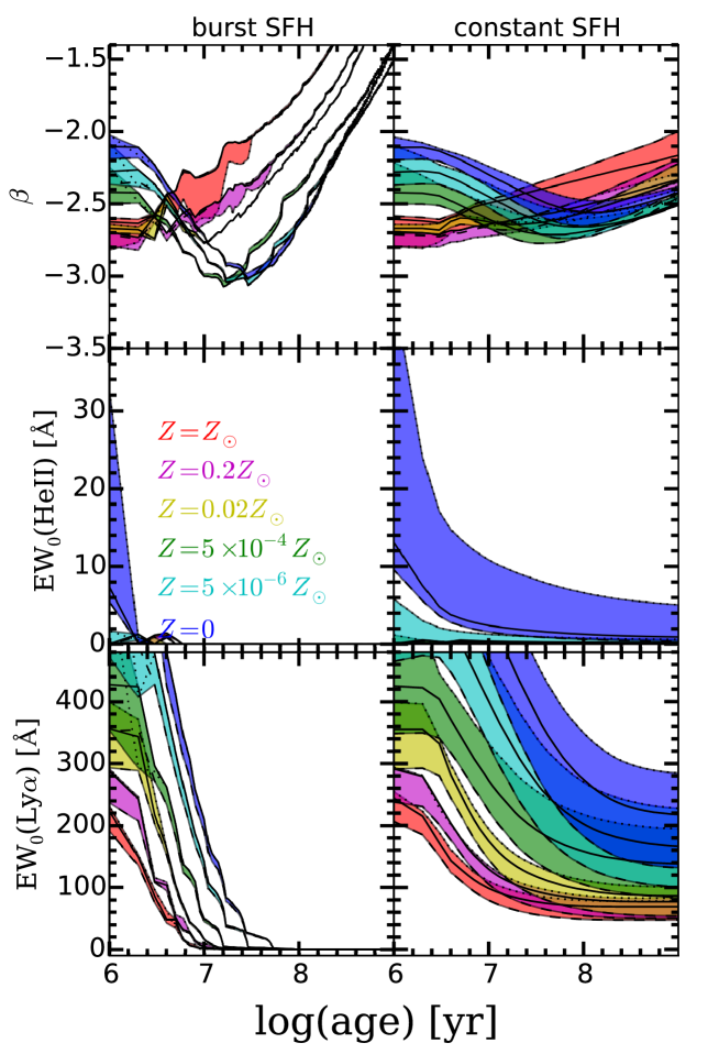
Figure 10: Theoretical evolutions of $\beta$, EW₀(Heii), and EW₀(Ly$\alpha$) values. The left and right panels are the results for the burst SFH and constant SFH, respectively. For each panel, the solid, dotted, and dashed lines correspond to the IMFs of A, B, and C, respectively (Table 7). The blue, cyan, green, yellow, magenta, and red regions denote evolution ranges traced by the IMFs for metallicities of $Z=0$, $5\times 10^{-6}$ $Z_{\odot}$, $5\times 10^{-4}$ $Z_{\odot}$, $0.02$ $Z_{\odot}$, $0.2$ $Z_{\odot}$, and $1.0$ $Z_{\odot}$, respectively.

Table 7: Summary of IMF Model Parameters

Model ID	IMF	Line type	$M_{\rm low}$	$M_{\rm up}$	$\alpha$
			($M_{\rm\odot}$)	($M_{\rm\odot}$)
(1)	(2)	(3)	(4)	(5)	(6)
A	Salpeter	solid	$1$	$100$	$2.35$
B	Salpeter	dotted	$100$	$500$	$2.35$
C	Scalo	dashed	$1$	$100$	$2.75$

(1) Model ID; (2) IMF; (3) Line style in Fig. 10; (4) and (5)

Lower and upper mass cut-off values; and (6) IMF slope value.

4.3.2 Comparisons of the Observational Constraints with the Models

Figures 11 $-$ 13 compare the observational constraints of $\beta$, EW₀(Heii), and EW₀(Ly$\alpha$) with the models. In these figures, gray shaded regions show the observed ranges of the three quantities. In the top panels, we show the intrinsic UV continuum slopes, $\beta_{\rm 1800-2200}$, for fair comparisons to the models (§3.2). In the second top panels, we present the upper limits of EW₀(Heii) (§3.4). The upper limits of EW₀(Heii) are obtained except for COSMOS-08501. As can be seen, these values are not strong enough to place constraints on the stellar age and metallicity. In the bottom panels, it should be noted that the models of Schaerer (2003) and Raiter et al. (2010) do not take into account the effects of Ly$\alpha$ scattering/absorption in the ISM and IGM. Thus, in Figures 11 $-$ 13, we plot the EW₀(Ly$\alpha$) values (§3.2) as the lower limits of the intrinsic EW₀(Ly$\alpha$) values for fair comparisons to the models.

In Figures 14 and 15, we plot the two ranges of the stellar ages and metallicities given by the $\beta$ and EW₀(Ly$\alpha$) values. The overlapped ranges of the two are adopted as the stellar ages and metallicities. Figures 14 and 15 clearly demonstrate that the combination of $\beta$ and EW₀(Ly$\alpha$) is powerful to constrain the stellar age and metallicity. Table 8 summarizes the permitted ranges of the stellar ages and metallicities of our LAEs. In Table 8, we find that our LAEs have generally low metallicities of $Z\lesssim 0.2Z_{\rm\odot}$. Interestingly, it is implied that at least a half of our large EW₀(Ly$\alpha$) LAEs would have young stellar ages of $\lesssim 20$ Myr and very low metallicities of $Z<0.02$ $Z_{\rm\odot}$ (possibly $Z\lesssim 5\times 10^{-4}$ $Z_{\rm\odot}$) regardless of the SFH. In Figure 14, we cannot obtain the stellar age and metallicity that simultaneously satisfy the $\beta$ and EW₀(Ly$\alpha$) values of COSMOS-41547. This object has an exceptionally large correction factor for $\beta_{\rm obs.1800-2200}$, $-1.25^{+0.20}_{-0.35}$, compared to the median correction factor of $-0.1\pm 0.2$ (§3.2). This is due to its large dust extinction value, $E(B-V)_{\rm*}=0.25^{+0.04}_{-0.07}$ (Table 3). Therefore, the stellar age and metallicity of COSMOS-41547 would be exceptionally affected by the systematic uncertainty discussed in §3.2. In §4.4, we consider other scenarios for the reason why the models have failed to constrain the stellar age and metallicity of COSMOS-41547.

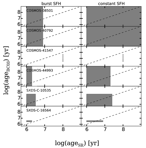
Figure 16: Comparisons of the two stellar ages of our LAEs, the one derived from SED fitting, age_BC03 (§3.1), and the other from the comparisons of observables to the models of Schaerer (2003) and Raiter et al. (2010), age_SR. For COSMOS-41547 whose age_SR cannot be constrained (see the text), the vertical dashed-line shows the range of age_SED. In the left (right) panels, the age_SR values are obtained assuming the burst (constant) SFH. In each panel, the gray shaded region denotes the $1\sigma$ ranges of the two stellar ages. The dashed line indicates the one-to-one relation.

Figure 16 compares the two stellar ages, the one derived from SED fitting (§3.1) and the other obtained with the models of Schaerer (2003) and Raiter et al. (2010). The former and the latter stellar ages are referred to as age_BC03 and age_SR, respectively. The age_BC03 value is determined by past star-formation activities. This is because the age_BC03 value is estimated from the photometric data that cover the rest-frame optical wavelength. In contrast, the age_SR value represents the age of the most recent star burst activity. This is due to the fact that the age_SR value is obtained from the rest-frame UV data alone. We find that the two stellar ages are consistent with each other within $1\sigma$ uncertainties regardless of the SFH. However, there is an exception, SXDS-C-16564 in the burst SFH case. In this case, the two stellar ages are consistent with each other within $2\sigma$ uncertainties. Among the two stellar ages, we adopt the age_SR values as the stellar ages of our LAEs. This is because the age_SR values are more realistic than the age_BC03 values in the sense that the age_SR values are estimated with no assumption on the metallicity value.

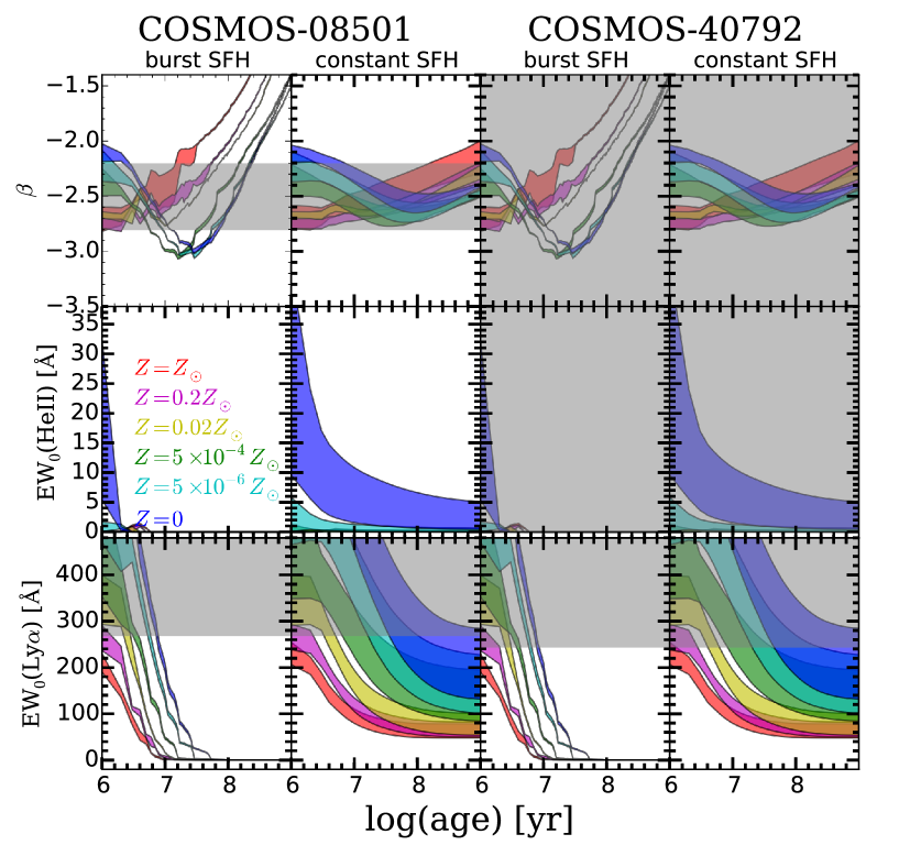
Figure 11: Comparisons of the observational constraints of $\beta$, EW₀(Heii), and EW₀(Ly$\alpha$) with the models for COSMOS-08501 and COSMOS-40792. For each object, the left and right panels show the results for the burst SFH and constant SFH, respectively. The color codes for the different metallicities are the same as those in Fig. 10. The horizontal gray shaded regions indicate the ranges of the observed quantities. In the top panels, we plot intrinsic $\beta$ values, $\beta_{\rm 1800-2200}$ (§3.2), that are corrected for dust attenuation effects on $\beta$. In the bottom panels, we plot EW₀(Ly$\alpha$) values (Table 4) as the lower limits of the intrinsic EW₀(Ly$\alpha$) values. This is because the models of Schaerer (2003) and Raiter et al. (2010) do not take into account the effects of Ly$\alpha$ scattering/absorption in the ISM and IGM.

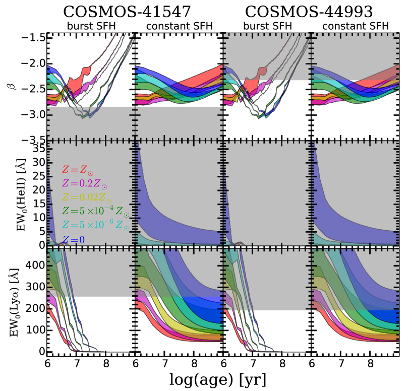
Figure 12: Same as Fig. 11 for COSMOS-41547 and COSMOS-44993.

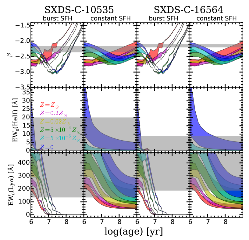
Figure 13: Same as Fig. 11 for SXDS-C-10535 and SXDS-C-16564.

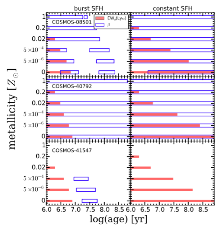
Figure 14: Left and right panels show permitted ranges of the stellar age and metallicity in the burst SFH and constant SFH, respectively, for COSMOS-08501, COSMOS-40792, and COSMOS-41547. The red filled squares and blue open squares denote the permitted ranges derived from the EW₀(Ly$\alpha$) and $\beta$ values, respectively. The overlapped regions of the red filled squares and blue open squares are the final constraints on the the stellar mass and metallicity.

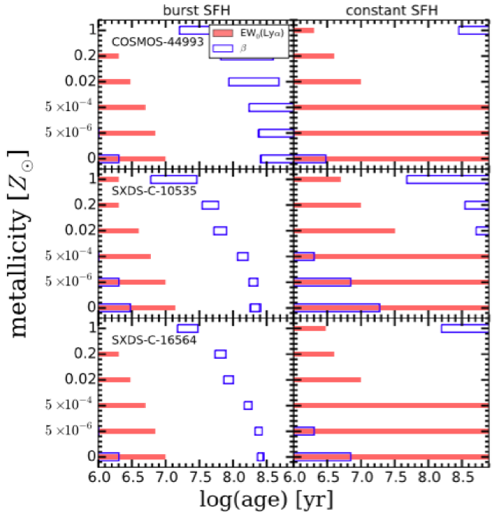
Figure 15: Same as Fig. 14 for COSMOS-44993, SXDS-C-10535, and SXDS-C-16564.

Table 8: Summary of Stellar age and Metallicity of Our LAEs

Object ID	SFH	stellar age
(1)	(2)	(3)
		$Z/Z_{\rm\odot}$ = 0	$5\times 10^{-6}$	$5\times 10^{-4}$	0.02	0.2	1.0
COSMOS-08501	burst	$3-8$ Myr	$<5$ Myr	$<3$ Myr	$<2$ Myr	$-$	$-$
	constant	$4-10^{3}$ Myr	$<100$ Myr	$<25$ Myr	$<5$ Myr	$<2$ Myr	$-$
COSMOS-40792	burst	$<8$ Myr	$<6.5$ Myr	$<5$ Myr	$<3.5$ Myr	$<2$ Myr	$-$
	constant	$<10^{3}$ Myr	$<250$ Myr	$<40$ Myr	$<6.5$ Myr	$<2$ Myr	$-$
COSMOS-41547	burst	$-$	$-$	$-$	$-$	$-$	$-$
	const	$-$	$-$	$-$	$-$	$-$	$-$
COSMOS-44993	burst	$<3.5$ Myr	$<2$ Myr	$-$	$-$	$-$	$-$
	constant	$<20$ Myr	$<8$ Myr	$<3$ Myr	$-$	$-$	$-$
SXDS-C-10535	burst	$<3.5$ Myr	$<2$ Myr	$-$	$-$	$-$	$-$
	constant	$<25$ Myr	$<10$ Myr	$<2$ Myr	$-$	$-$	$-$
SXDS-C-16564	burst	$<2$ Myr	$-$	$-$	$-$	$-$	$-$
	constant	$<8$ Myr	$<2$ Myr	$-$	$-$	$-$	$-$

(1) Object ID; (2) Star formation history; and (3) Permitted range of the stellar age for the each metallicity in the second row.

4.3.3 Limitations of Our Discussion

We have derived the stellar ages and metallicities of our LAEs with two assumptions. First, we have presumed the Case B recombination. As pointed out by Raiter et al. (2010) and Dijkstra (2014), significant departures from Case B are expected at the low metallicity range of $Z\lesssim 0.03$ $Z_{\rm\odot}$ (see also Mas-Ribas et al. 2016). The departures can contribute to strong Ly$\alpha$ emission up to EW₀(Ly$\alpha$) $\sim 4000$ Å because of (i) the increased importance of collisional excitation at the high gas temperature (ii) and the hard ionizing spectra emitted by metal poor stars (Dijkstra 2014). The departures can also contribute to weak Heii emission compared to Case B (Raiter et al. 2010). Thus, the constraints on the stellar age and metallicity may not be correct. Second, we have assumed a limited number of IMFs. Raiter et al. (2010) have argued that large uncertainties remain in the shape of the IMF of the metal-poor or metal-free stars. Therefore, the constraints on the stellar age and metallicity suffer from uncertainties due to the shape of the IMF.

4.4 Other Scenarios of the Large EW₀(Ly$\alpha$)

We have studied properties of our LAEs assuming that all Ly$\alpha$ photons are produced by star forming activities. However, several other mechanisms can also generate Ly$\alpha$ photons. These include photoionization induced by (i) AGN activities (e.g., Malhotra & Rhoads 2002; Dawson et al. 2004) or (ii) external UV background sources such as QSOs (QSO fluorescence: e.g., Cantalupo et al. 2005, 2012). In addition, Ly$\alpha$ photons can be produced by collisional excitation due to (iii) strong outflows (shock heating: e.g., Taniguchi & Shioya 2000; Mori et al. 2004; Otí-Floranes et al. 2012) or (iv) inflows of gas into a galaxy (gravitational cooling: e.g., Haiman et al. 2000; Dijkstra & Loeb 2009; Rosdahl & Blaizot 2012). These mechanisms can enhance the Ly$\alpha$ production, leading to large EW₀(Ly$\alpha$) values. Moreover, (v) if a galaxy has a clumpy ISM, where dust grains are shielded by Hi gas, EW₀(Ly$\alpha$) values can be apparently boosted. This is because Ly$\alpha$ photons are resonantly scattered on the surfaces of clouds without being absorbed by dust, while continuum photons are absorbed through dusty gas clouds (e.g., Neufeld 1991; Hansen & Oh 2006; Kobayashi et al. 2010; Laursen et al. 2013; Gronke & Dijkstra 2014). We examine these five hypotheses.

AGN activities: AGN activities can enhance EW₀(Ly$\alpha$). However, we have confirmed that our LAEs do not host an AGN both on the individual and stacked bases (§2.4). The scenario is unlikely.

QSO fluorescence: According to the result of Cantalupo et al. (2005), QSOs can photoionize the outer layer of the ISM of nearby galaxies, enhancing EW₀(Ly$\alpha$) of the nearby galaxy. We examine this hypothesis in two ways. First, we have confirmed that there are no QSOs around any of our LAEs. Second, as discussed in Kashikawa et al. (2012), objects with fluorescent Ly$\alpha$ often do not have stellar-continuum counterparts. However, our LAEs clearly have stellar continuum counterparts (Table 2). Therefore, we conclude that the QSO fluorescence hypothesis is unlikely.

Shock heating: Shock heating caused by strong outflows can produce Ly$\alpha$ photons (Taniguchi & Shioya 2000; Mori et al. 2004; Otí-Floranes et al. 2012). In this case, the Ly$\alpha$ morphology is expected to be spatially extended (Haiman et al. 2000; Taniguchi et al. 2015). However, our LAEs have spatially compact Ly$\alpha$ morphologies (§2.1). To obtain a definitive conclusion, it is useful to perform follow-up observations targeting [Sii] and [Nii] emission lines. This is because [Sii] and [Nii] emission lines are sensitive to the presence of shock heating (e.g., Newman et al. 2012). It is also interesting to perform follow-up observations targeting metal absorption lines. With blue-shifts of metal absorption lines with respect to the systemic redshifts, we can examine if outflow velocities are large enough to cause shock heating in our LAEs (e.g., Shapley et al. 2003; Shibuya et al. 2014b; Rivera-Thorsen et al. 2015).

Gravitational cooling: Ly$\alpha$ photons can be also generated by gravitational cooling. The gravitational binding energy of gas inflowing into a galaxy is converted into thermal energy, then released as Ly$\alpha$ emission. Ly$\alpha$ emission produced by gravitational cooling is predicted to be spatially extended (Rosdahl & Blaizot 2012). The compact Ly$\alpha$ morphologies of our LAEs do not favor the hypothesis. Deep H$\alpha$ data would help us to obtain a definitive conclusion. In the case of gravitational cooling, we expect a very high flux ratio of Ly$\alpha$ and H$\alpha$ lines, Ly$\alpha$/H$\alpha\sim 100$ (Dijkstra 2014). This high flux ratio can be distinguished from the ratio for the Case B recombination, Ly$\alpha$/H$\alpha=8.7$.

Clumpy ISM: Finally, the gas distribution of LAEs may not be smooth. Duval et al. (2014) have theoretically investigated the condition of an ISM to boost EW₀(Ly$\alpha$) values. The EW₀(Ly$\alpha$) value can be boosted if a galaxy has an almost static (galactic outflows $<200$ km s^-1), clumpy, and very dusty ($E(B-V)_{\rm*}>0.30$) ISM. The small median dust extinction value of our LAEs, $E(B-V)_{\rm*}=0.02^{+0.04}_{-0.02}$, would be at odds with the hypothesis.

In summary, no clear evidence of the five scenarios has been found in our LAEs.

In §4.3.2, we have shown that we cannot constrain the stellar age and metallicity of COSMOS-41547. One might think that the result is affected by e.g., a hidden AGN or collisional excitation. From Figure 12, we have found that we can constrain the stellar age and metallicity of this object if more than $60\%$ of the observed Ly$\alpha$ flux is contributed from these additional mechanisms. If this is the case, we should see clear evidence of these effects. However, as we have shown, we do not see any clear evidence of these. Therefore, while the additional mechanisms could explain the failure of our method, the failure is most likely due to the systematic uncertainty as described in §4.3.2.

5 SUMMARY AND CONCLUSION

We have presented physical properties of spectroscopically confirmed LAEs with very large EW₀(Ly$\alpha$) values. We have identified six LAEs selected from $\sim 3000$ LAEs at $z\sim 2$ with reliable measurements of EW₀(Ly$\alpha$) $\simeq 200-400$ Å given by careful continuum determinations with our deep photometric and spectroscopic data. These LAEs do not have signatures of AGN. Our main results are as follows.

• We have performed SED fitting to derive physical quantities such as the stellar mass and dust extinction. Our LAEs have stellar masses of $M_{\rm*}=10^{7-8}M_{\rm\odot}$ with a median value of $7.1^{+4.8}_{-2.8}\times 10^{7}M_{\rm\odot}$. The stellar masses of our LAEs is significantly smaller than those of small EW₀(Ly$\alpha$) LAEs at $z\sim 2$, $M_{\rm*}=10^{8-10}M_{\rm\odot}$ (Nakajima et al. 2012; Oteo et al. 2015; Shimakawa et al. 2016). Our LAEs have stellar dust extinction values ranging from $E(B-V)_{\rm*}=0.00$ to $0.25$ with a median value of $0.02^{+0.04}_{-0.02}$. The median value is lower than that of small EW₀(Ly$\alpha$) LAEs at $z\sim 2$, $E(B-V)_{\rm*}=0.2-0.3$ (Guaita et al. 2011; Nakajima et al. 2012; Oteo et al. 2015).

• By modeling FUV photometric data with no apriori assumption on $\beta$ values, we find that our LAEs have EW₀(Ly$\alpha$) values ranging from EW₀(Ly$\alpha$) $=160$ to $357$ Å, with a large mean value of $252\pm 30$ Å. This confirms that LAEs with EW₀(Ly$\alpha$) $\gtrsim 200$ Å exist. Our LAEs are characterized by the median values of $L({\rm Ly\alpha})=3.7\times 10^{42}$ erg s^-1 and $M_{\rm UV}=-18.0$ as well as the small medan UV continuum slope of $\beta=-2.5\pm 0.2$.

• Using stellar masses and SFRs derived from SED fitting, we have investigated our LAEs’ star-formation mode. With a high median sSFR ($\equiv$ SFR/$M_{\rm*}$) of $\sim 100$ Gyr^-1, our LAEs typically lie above the lower-mass extrapolation of the SFMS $z\sim 2$ defined by massive galaxies ($M_{\rm*}>10^{10}M_{\rm\odot}$). An interpretation of the offset toward high sSFR is that our LAEs are in the burst star-formation mode. However, the offset can be also due to (i) a different slope of the SFMS at the low stellar mass range or (ii) a selection effect of choosing galaxies with bright emission lines (i.e., high SFRs) at the low stellar mass range.

• We have estimated the Ly$\alpha$ escape fraction, $f^{\rm Ly\alpha}_{\rm esc}$. For the three objects that have relatively small errors, the median value is calculated to be $f^{\rm Ly\alpha}_{\rm esc}=0.68\pm 0.30$. The high $f^{\rm Ly\alpha}_{\rm esc}$ value of our LAEs can be explained by the small dust content inferred from the small $E(B-V)_{\rm*}$ and $\beta$ values.

• Our large EW₀(Ly$\alpha$) LAEs have a small mean FWHM_int(Ly$\alpha$) of $212\pm 32$ km s^-1, significantly smaller than those of small EW₀(Ly$\alpha$) LAEs and LBGs at the similar redshift. Combined with small EW₀(Ly$\alpha$) LAEs and LBGs in the literature, we have statistically shown that there is an anti-correlation between EW₀(Ly$\alpha$) and FWHM_int(Ly$\alpha$). The small FWHM_int(Ly$\alpha$) values of our LAEs can be explained either by (i) low $N_{\rm HI}$ values in the ISM, (ii) low neutral-gas covering fractions of the ISM, or (iii) small dynamical masses.

• We have placed constraints on the stellar ages and metallicities of our LAEs with the stellar evolution models of Schaerer (2003) and Raiter et al. (2010). Our observational constraints of the large EW₀(Ly$\alpha$), the small $\beta$, and EW₀(Heii) imply that at least half of our large EW₀(Ly$\alpha$) LAEs would have young stellar ages of $\lesssim 20$ Myr and very low metallicities of $Z<0.02$ $Z_{\rm\odot}$ regardless of the SFH.

• We have investigated five other scenarios of the large EW₀(Ly$\alpha$) values of our LAEs: AGN activities, QSO fluorescence, shock heating, gravitational cooling, and the presence of the clumpy ISM. Our sample does not show any clear evidence of these hypotheses.

Among the results, the small $E(B-V)_{\rm*}$ and $\beta$ values are consistent with the high $f^{\rm Ly\alpha}_{\rm esc}$ values of our LAEs. The high $f^{\rm Ly\alpha}_{\rm esc}$ values are also consistent with the small FWHM(Ly$\alpha$) values indicative of the low Hi column densities. We conclude that all of the low stellar masses, the young stellar ages, the low metallicities, and the high sSFR values are consistent with an idea that our large EW₀(Ly$\alpha$) LAEs represent the early stage of the galaxy formation and evolution with intense star-forming activities. The number of large EW₀(Ly$\alpha$) LAEs in this study is admittedly small. Hyper-Sprime Cam, a wide-field camera installed on Subaru, will be useful to increase the number of EW₀(Ly$\alpha$) LAEs at various redshifts.

References

- Adams et al. (2011) Adams, J. J., et al. 2011, ApJS, 192, 5
- Alavi et al. (2014) Alavi, A., et al. 2014, ApJ, 780, 143
- Ando et al. (2006) Ando, M., Ohta, K., Iwata, I., Akiyama, M., Aoki, K., & Tamura, N. 2006, ApJ, 645, L9
- Atek et al. (2008) Atek, H., Kunth, D., Hayes, M., Östlin, G., & Mas-Hesse, J. M. 2008, A&A, 488, 491
- Atek et al. (2009) Atek, H., Kunth, D., Schaerer, D., Hayes, M., Deharveng, J. M., Östlin, G., & Mas-Hesse, J. M. 2009, A&A, 506, L1
- Atek et al. (2014) Atek, H., Kunth, D., Schaerer, D., Mas-Hesse, J. M., Hayes, M., Östlin, G., & Kneib, J.-P. 2014, A&A, 561, A89
- Baldwin et al. (1981) Baldwin, J. A., Phillips, M. M., & Terlevich, R. 1981, PASP, 93, 5
- Bertin & Arnouts (1996) Bertin, E., & Arnouts, S. 1996, A&AS, 117, 393
- Bouwens et al. (2009) Bouwens, R. J., et al. 2009, ApJ, 705, 936
- Bowler et al. (2016) Bowler, R. A. A., McLure, R. J., Dunlop, J. S., McLeod, D. J., Stanway, E. R., Eldridge, J. J., & Jarvis, M. J. 2016, 2016arXiv160900727B
- Brammer et al. (2012) Brammer, G. B., et al. 2012, ApJS, 200, 13
- Bruzual & Charlot (2003) Bruzual, G., & Charlot, S. 2003, MNRAS, 344, 1000
- Calzetti et al. (2000) Calzetti, D., Armus, L., Bohlin, R. C., Kinney, A. L., Koornneef, J., & Storchi-Bergmann, T. 2000, ApJ, 533, 682
- Cantalupo et al. (2012) Cantalupo, S., Lilly, S. J., & Haehnelt, M. G. 2012, MNRAS, 425, 1992
- Cantalupo et al. (2005) Cantalupo, S., Porciani, C., Lilly, S. J., & Miniati, F. 2005, ApJ, 628, 61
- Cassata et al. (2015) Cassata, P., et al. 2015, A&A, 573, A24
- Charlot & Fall (1993) Charlot, S., & Fall, S. M. 1993, ApJ, 415, 580
- Ciardullo et al. (2012) Ciardullo, R., et al. 2012, ApJ, 744, 110
- Ciardullo et al. (2014) Ciardullo, R., et al. 2014, ApJ, 796, 64
- Cowie & Hu (1998) Cowie, L. L., & Hu, E. M. 1998, AJ, 115, 1319
- Daddi et al. (2007) Daddi, E., et al. 2007, ApJ, 670, 156
- Dawson et al. (2004) Dawson, S., et al. 2004, ApJ, 617, 707
- Dijkstra (2014) Dijkstra, M. 2014, PASA, 31, e040
- Dijkstra & Loeb (2009) Dijkstra, M., & Loeb, A. 2009, MNRAS, 396, 377
- Duval et al. (2014) Duval, F., Schaerer, D., Östlin, G., & Laursen, P. 2014, A&A, 562, A52
- Elvis et al. (2009) Elvis, M., et al. 2009, ApJS, 184, 158
- Erb et al. (2016) Erb, D. K., Pettini, M., Steidel, C. C., Strom, A. L., Rudie, G. C., Trainor, R. F., Shapley, A. E., & Reddy, N. A. 2016, ArXiv e-prints
- Erb et al. (2006) Erb, D. K., Steidel, C. C., Shapley, A. E., Pettini, M., Reddy, N. A., & Adelberger, K. L. 2006, ApJ, 646, 107
- Erb et al. (2014) Erb, D. K., et al. 2014, ApJ, 795, 33
- Finkelstein et al. (2011) Finkelstein, S. L., et al. 2011, ApJ, 729, 140
- Furusawa et al. (2008) Furusawa, H., et al. 2008, ApJS, 176, 1
- Grogin et al. (2011) Grogin, N. A., et al. 2011, ApJS, 197, 35
- Gronke & Dijkstra (2014) Gronke, M., & Dijkstra, M. 2014, MNRAS, 444, 1095
- Gronke & Dijkstra (2016) Gronke, M., & Dijkstra, M. 2016, ApJ, 826, 14
- Gronwall et al. (2007) Gronwall, C., et al. 2007, ApJ, 667, 79
- Guaita et al. (2011) Guaita, L., et al. 2011, ApJ, 733, 114
- Hagen et al. (2016) Hagen, A., et al. 2016, ApJ, 817, 79
- Haiman & Rees (2001) Haiman, Z., & Rees, M. J. 2001, ApJ, 556, 87
- Haiman et al. (2000) Haiman, Z., Spaans, M., & Quataert, E. 2000, ApJ, 537, L5
- Hansen & Oh (2006) Hansen, M., & Oh, S. P. 2006, MNRAS, 367, 979
- Hashimoto et al. (2013) Hashimoto, T., Ouchi, M., Shimasaku, K., Ono, Y., Nakajima, K., Rauch, M., Lee, J., & Okamura, S. 2013, ApJ, 765, 70
- Hashimoto et al. (2015) Hashimoto, T., et al. 2015, ApJ, 812, 157
- Hathi et al. (2013) Hathi, N. P., et al. 2013, ApJ, 765, 88
- Hathi et al. (2016) Hathi, N. P., et al. 2016, A&A, 588, 26
- Hayes et al. (2011) Hayes, M., Schaerer, D., Östlin, G., Mas-Hesse, J. M., Atek, H., & Kunth, D. 2011, ApJ, 730, 8
- Hayes et al. (2010) Hayes, M., et al. 2010, Nature, 464, 562
- Henry et al. (2015) Henry, A., Scarlata, C., Martin, C. L., & Erb, D. 2015, ApJ, 809, 19
- Jones et al. (2013) Jones, T. A., Ellis, R. S., Schenker, M. A., & Stark, D. P. 2013, ApJ, 779, 52
- Karman et al. (2016) Karman, W., et al. 2016, 2016arXiv160601471K
- Kashikawa et al. (2012) Kashikawa, N., et al. 2012, ApJ, 761, 85
- Kennicutt (1998) Kennicutt, Jr., R. C. 1998, ARA&A, 36, 189
- Kobayashi et al. (2010) Kobayashi, M. A. R., Totani, T., & Nagashima, M. 2010, ApJ, 708, 1119
- Koekemoer et al. (2011) Koekemoer, A. M., et al. 2011, ApJS, 197, 36
- Konno et al. (2016) Konno, A., Ouchi, M., Nakajima, K., Duval, F., Kusakabe, H., Ono, Y., & Shimasaku, K. 2016, ApJ, 823, 20
- Kunth et al. (1998) Kunth, D., Mas-Hesse, J. M., Terlevich, E., Terlevich, R., Lequeux, J., & Fall, S. M. 1998, A&A, 334, 11
- Kusakabe et al. (2015) Kusakabe, H., Shimasaku, K., Nakajima, K., & Ouchi, M. 2015, ApJ, 800, L29
- Laursen et al. (2013) Laursen, P., Duval, F., & Östlin, G. 2013, ApJ, 766, 124
- Laursen et al. (2011) Laursen, P., Sommer-Larsen, J., & Razoumov, A. O. 2011, ApJ, 728, 52
- Madau (1995) Madau, P. 1995, ApJ, 441, 18
- Madau & Dickinson (2014) Madau, P., & Dickinson, M. 2014, ARA&A, 52, 415
- Malhotra & Rhoads (2002) Malhotra, S., & Rhoads, J. E. 2002, ApJ, 565, L71
- Malhotra & Rhoads (2004) Malhotra, S., & Rhoads, J. E. 2004, ApJ, 617, L5
- Mas-Ribas et al. (2016) Mas-Ribas, L., Dijkstra, M., & Forero-Romero, J. E., 2016, arXiv160902150M
- Matsuda et al. (2004) Matsuda, Y., et al. 2004, AJ, 128, 569
- Matthee et al. (2016) Matthee, J., Sobral, D., Oteo, I., Best, P., Smail, I., Röttgering, H., & Paulino-Afonso, A. 2016, MNRAS, 458, 449
- Mawatari et al. (2012) Mawatari, K., Yamada, T., Nakamura, Y., Hayashino, T., & Matsuda, Y. 2012, ApJ, 759, 133
- Meurer et al. (1999) Meurer, G. R., Heckman, T. M., & Calzetti, D. 1999, ApJ, 521, 64
- Momose et al. (2014) Momose, R., et al. 2014, MNRAS, 442, 110
- Momose et al. (2016) Momose, R., et al. 2016, MNRAS, 457, 2318
- Mori et al. (2004) Mori, M., Umemura, M., & Ferrara, A. 2004, ApJ, 613, L97 Møller, P. and Warren, S. J.,
- Møller & Warren (1998) Møller, P. and Warren, S. J., 1998, MNRAS, 299, 661
- Nagao et al. (2005) Nagao, T., Motohara, K., Maiolino, R., Marconi, A., Taniguchi, Y., Aoki, K., Ajiki, M., & Shioya, Y. 2005, ApJ, 631, L5
- Nakajima & Ouchi (2014) Nakajima, K., & Ouchi, M. 2014, MNRAS, 442, 900
- Nakajima et al. (2013) Nakajima, K., Ouchi, M., Shimasaku, K., Hashimoto, T., Ono, Y., & Lee, J. C. 2013, ApJ, 769, 3
- Nakajima et al. (2012) Nakajima, K., et al. 2012, ApJ, 745, 12
- Neufeld (1991) Neufeld, D. A. 1991, ApJ, 370, L85
- Newman et al. (2012) Newman, S. F., et al. 2012, ApJ, 761, 43
- Nilsson et al. (2011) Nilsson, K. K., Östlin, G., Møller, P., Möller-Nilsson, O., Tapken, C., Freudling, W., & Fynbo, J. P. U. 2011, A&A, 529, A9
- Nilsson et al. (2007) Nilsson, K. K., et al. 2007, A&A, 471, 71
- Oke & Gunn (1983) Oke, J. B., & Gunn, J. E. 1983, ApJ, 266, 713
- Ono et al. (2010a) Ono, Y., Ouchi, M., Shimasaku, K., Dunlop, J., Farrah, D., McLure, R., & Okamura, S. 2010a, ApJ, 724, 1524
- Ono et al. (2010b) Ono, Y., et al. 2010b, MNRAS, 402, 1580
- Oteo et al. (2015) Oteo, I., Sobral, D., Ivison, R. J., Smail, I., Best, P. N., Cepa, J., & Pérez-García, A. M. 2015, MNRAS, 452, 2018
- Otí-Floranes et al. (2012) Otí-Floranes, H., Mas-Hesse, J. M., Jiménez-Bailón, E., Schaerer, D., Hayes, M., Östlin, G., Atek, H., & Kunth, D. 2012, A&A, 546, A65
- Ouchi et al. (2003) Ouchi, M., et al. 2003, ApJ, 582, 60
- Ouchi et al. (2004) Ouchi, M., et al. 2004, ApJ, 611, 660
- Ouchi et al. (2008) Ouchi, M., et al. 2008, ApJS, 176, 301
- Ouchi et al. (2010) Ouchi, M., et al. 2010, ApJ, 723, 869
- Pettini et al. (1998) Pettini, M., Kellogg, M., Steidel, C. C., Dickinson, M., Adelberger, K. L., & Giavalisco, M. 1998, ApJ, 508, 539
- Raiter et al. (2010) Raiter, A., Schaerer, D., & Fosbury, R. A. E. 2010, A&A, 523, A64
- Rhoads et al. (2000) Rhoads, J. E., Malhotra, S., Dey, A., Stern, D., Spinrad, H., & Jannuzi, B. T. 2000, ApJ, 545, L85
- Rivera-Thorsen et al. (2015) Rivera-Thorsen, T. E., et al. 2015, ApJ, 805, 14
- Rodighiero et al. (2011) Rodighiero, G., et al. 2011, ApJ, 739, L40
- Rosdahl & Blaizot (2012) Rosdahl, J., & Blaizot, J. 2012, MNRAS, 423, 344
- Salpeter (1955) Salpeter, E. E. 1955, ApJ, 121, 161
- Scalo (1986) Scalo, J. M. 1986, Fund. Cosmic Phys., 11, 1
- Schaerer (2002) Schaerer, D. 2002, A&A, 382, 28
- Schaerer (2003) Schaerer, D. 2003, A&A, 397, 527
- Schaerer & de Barros (2009) Schaerer, D., & de Barros, S. 2009, A&A, 502, 423
- Schaerer, de Barros, & Sklias (2013) Schaerer, D., de Barros, S., & Sklias, P., 2013, A&A, 549, 4
- Schinnerer et al. (2010) Schinnerer, E., et al. 2010, ApJS, 188, 384
- Schlegel et al. (1998) Schlegel, D. J., Finkbeiner, D. P., & Davis, M. 1998, ApJ, 500, 525
- Shapley et al. (2003) Shapley, A. E., Steidel, C. C., Pettini, M., & Adelberger, K. L. 2003, ApJ, 588, 65
- Shibuya et al. (2014a) Shibuya, T., Ouchi, M., Nakajima, K., Yuma, S., Hashimoto, T., Shimasaku, K., Mori, M., & Umemura, M. 2014a, ApJ, 785, 64
- Shibuya et al. (2014b) Shibuya, T., et al. 2014b, ApJ, 788, 74
- Shimakawa et al. (2016) Shimakawa, R., et al. 2016, ArXiv e-prints
- Shimasaku et al. (2006) Shimasaku, K., et al. 2006, PASJ, 58, 313
- Skelton et al. (2014) Skelton, R. E., et al. 2014, ApJS, 214, 24
- Sobral et al. (2015) Sobral, D., Matthee, J., Darvish, B., Schaerer, D., Mobasher, B., Röttgering, H. J. A., Santos, S., & Hemmati, S. 2015, ApJ, 808, 139
- Song et al. (2014) Song, M., et al. 2014, ApJ, 791, 3
- Speagle et al. (2014) Speagle, J. S., Steinhardt, C. L., Capak, P. L., & Silverman, J. D. 2014, ApJS, 214, 15
- Stark et al. (2010) Stark, D. P., Ellis, R. S., Chiu, K., Ouchi, M., & Bunker, A. 2010, MNRAS, 408, 1628
- Stark et al. (2015) Stark, D. P., et al. 2015, MNRAS, 450, 1846
- Steidel et al. (2000) Steidel, C. C., Adelberger, K. L., Shapley, A. E., Pettini, M., Dickinson, M., & Giavalisco, M. 2000, ApJ, 532, 170
- Steidel et al. (2011) Steidel, C. C., Bogosavljević, M., Shapley, A. E., Kollmeier, J. A., Reddy, N. A., Erb, D. K., & Pettini, M. 2011, ApJ, 736, 160
- Steidel et al. (2010) Steidel, C. C., Erb, D. K., Shapley, A. E., Pettini, M., Reddy, N., Bogosavljević, M., Rudie, G. C., & Rakic, O. 2010, ApJ, 717, 289
- Taniguchi & Shioya (2000) Taniguchi, Y., & Shioya, Y. 2000, ApJ, 532, L13
- Taniguchi et al. (2015) Taniguchi, Y., et al. 2015, ApJ, 809, L7
- Tapken et al. (2007) Tapken, C., Appenzeller, I., Noll, S., Richling, S., Heidt, J., Meinköhn, E., & Mehlert, D. 2007, A&A, 467, 63
- Trainor et al. (2015) Trainor, R. F., Steidel, C. C., Strom, A. L., & Rudie, G. C. 2015, ApJ, 809, 89
- Verhamme et al. (2015) Verhamme, A., Orlitová, I., Schaerer, D., & Hayes, M. 2015, A&A, 578, A7
- Villar-Martín et al. (2007) Villar-Martín, M., Humphrey, A., De Breuck, C., Fosbury, R., Binette, L., & Vernet, J. 2007, MNRAS, 375, 1299
- Wang et al. (2009) Wang, J.-X., Malhotra, S., Rhoads, J. E., Zhang, H.-T., & Finkelstein, S. L. 2009, ApJ, 706, 762
- Willmarth & Barnes (1994) Willmarth, D., & Barnes, J. 1994, Central Computer Services, NOAO
- Zheng et al. (2014) Zheng, Z.-Y., Wang, J.-X., Malhotra, S., Rhoads, J. E., Finkelstein, S. L., & Finkelstein, K. 2014, MNRAS, 439, 1101
- Zheng & Wallace (2014) Zheng, Z., & Wallace, J. 2014, ApJ, 794, 116