Moiré Assisted Fractional Quantum Hall State Spectroscopy

Abstract

Intra-Landau level excitations in the fractional quantum Hall regime are not accessible via optical absorption measurements. We point out that optical probes are enabled by the periodic potentials produced by a moiré pattern. Our observation is motivated by the recent observations of fractional quantum Hall incompressible states in moiré-patterned graphene on a hexagonal boron nitride substrate, and is theoretically based on $f-$sum rule considerations supplemented by a perturbative analysis of the influence of the moiré potential on many-body states.

I Introduction

When electrons in two-dimensions partially occupy a macroscopically degenerate Landau level (LL), the character of the ground state and of its excitations both change in a complex way as a function of filling factor $\nu$ and LL kinetic energy index $n$. The charged excitation gaps (chemical potential discontinuities) that appear at many rational LL filling factors are efficiently exposed by transport measurements becauseLesHouches they give rise to fractional quantum Hall (FQH) effects. It has however been a stumbling block in explorations of FQH physics that many other aspects of the uniquely subtle many-electron states are hidden from view, and in particular that excitations within a single LL of a two-dimensional electron system (2DES) are optically dark. In this article we propose an approach which can be used to make them visible.

When two van der Waals materials form a heterojunction, misalignment and lattice constant differences give rise to a periodic moiré pattern that makes all local observables periodic functions of position. Moiré patterns are particularly important when formed in graphene sheets because the high quality of these 2DESs helps make their influence dominate over random inhomogeneity induced by uncontrolled disorder. Moiré patterns formed in graphene on hexagonal boron nitride (hBN) and graphene on graphene have recently Hunt13 ; Dean13 ; Yu14 ; Dean15 ; TutucNew been successfully used to realize Hofstader butterfly systems with fractal band spectra that are extraordinarily sensitive to commensurability between magnetic-field and periodic potential area scales. Here we show that they also enable coupling between light and intra-LL collective excitations.

To illustrate our ideas we focus on the collective excitations of the strongest fractional quantum Hall incompressible states, those that occur at $\nu=1/3$ and $\nu=2/3$ which were first understood by Laughlin and are named in his honor. The collective excitations of these states are accurately described by the single-mode approximation of Girvin, MacDonald and PlatzmanGMP . Because of analogies between these excitations and the roton modes in superfluid helium, collective excitation of FQH states are known as magneto-rotons. Magneto-roton properties have been investigated using a variety of approaches, for example by using exact diagonalizationHaldane ; Jolicoeur16 methods or applying composite bosonsZhang91 or composite fermionsJain92 ideas, and continue to be actively studied. Recent advances include the identification of a connection to Hall viscosityHaldane09 ; Haldane12 and an analysis of their relationship to the stability of FQH statesSondhi13 .

The experimental observation of the intra-LL collective excitations of FQH states has been an ongoing challenge because of the absence in homogeneous fluids of dipole coupling between light and any intra-LL neutral excitation. Inelastic light scattering has provided indirect signatures of intra-LL collective excitationsWest93 ; West01 ; West05 ; West13 which are thought to be enabled by disorder which breaks translational symmetry and enables coupling between light and finite-momentum excitations, but does not allow for momentum resolution. We show below that weak moiré patterns expose collective excitations only at the moiré pattern reciprocal lattice wave vectors, which can be tuned by varying the van der Waals heterojunction twist angle.

Our paper is organized as follows. In Sec. II, we derive a strong magnetic field $f-$sum rule and use it to show quite generally that the contribution of intra-LL excitation to the optical conductivity is finite in the presence of a spatially varying potential. In Sec. III, we use perturbation theory to account for the influence of moiré potential on incompressible FQH states. The perturbative approach is valid when the periodic moiré potential is weak compared to the collective mode excitation energies. In Sec. IV, we also make a single mode approximation to provide an explicit expression for the optical conductivity of the $\nu=1/3$ FQHE states. Finally in Sec. V, we discuss possible experimental systems, including graphene/hBN and twisted transition metal dichalcogenides (TMD) bilayers.

II Strong Magnetic Field $f-$sum rule

We consider electrons in the lowest-LL and for the moment neglect possible spin or valley degrees of freedom. When projected to the lowest LL, the Hamiltonian includes only Coulomb interaction $\hat{H}_{C}$ and moiré potential $\hat{V}$ terms, and is given up to a constant by:

$$\hat{H} =\hat{H}_{C}+\hat{V},$$ (1)

$$\hat{H}_{C} =\frac{1}{2}\int\frac{d^{2}\mathbb{q}}{(2\pi)^{2}}v_{C}(\mathbb{q})\;\bar{\rho}_{-\mathbb{q}}\,\bar{\rho}_{\mathbb{q}},$$

$$\hat{V} =\sum_{\mathbb{G}}V_{\mathbb{G}}\bar{\rho}_{\mathbb{G}},$$

where

$$\bar{\rho}_{\mathbb{q}}=\sum_{j}\overline{\text{exp}[-i\mathbb{q}\cdot\mathbb{r}_{j}]}$$ (2)

is the LL projected density operator, and $v_{C}(\mathbb{q})=2\pi e^{2}/(\varepsilon|\mathbb{q}|)$ is the Coulombic electron-electron interaction. The potential $\hat{V}$ is produced by the moiré pattern, and is periodic as illustrated in Fig. 1(a). For graphene/hBNsublattice the spatial variation of $\hat{V}$ is accurately characterized by a Fourier expansion that includes only the six wave vectors in the first shell of moiré reciprocal lattice shown in Fig. 1(b).Bistritzer11 The summation over $\mathbb{G}$ in Eq. (1) is restricted to these six vectors. Because the potential is real and the moiré pattern has Falko13 three-fold rotational symmetry, we have the following constraints:

$$V_{\mathbb{G}_{1}}=V_{\mathbb{G}_{3}}=V_{\mathbb{G}_{5}}=V_{\mathbb{G}_{2}}^{*}=V_{\mathbb{G}_{4}}^{*}=V_{\mathbb{G}_{6}}^{*}.$$ (3)

The magnitude of $\mathbb{G}$ in the first shell can be varied by adjusting the twist angle $\theta$. For small $\theta$:

$$|\mathbb{G}|=\frac{4\pi}{\sqrt{3}a_{M}}\;,\;a_{M}\approx a/\sqrt{x^{2}+\theta^{2}},$$ (4)

where $a_{M}$ is the moiré periodicity, $x=|a^{\prime}-a|/a$, and $a$ and $a^{\prime}$ are the lattice constants of the two layersJung14 .

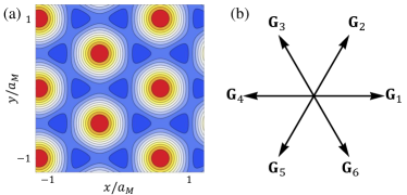
Figure 1: (Color online)(a) Schematic illustration of a periodic potential in real space due to a moiré pattern formed between 2D crystals with triangular Bravais lattices. (b) The first shell of moiré reciprocal lattice vectors.

The optical conductivity $\sigma(\omega)$ of a material can be probed by measuring optical reflection, transmission, or absorption. Theoretically, the longitudinal conductivity can be related to the density-density response function $\chi$ using

$$\sigma(\mathbb{q},\omega)=e^{2}\frac{i\omega}{|\mathbb{q}|^{2}}\Pi(\mathbb{q},\omega),$$ (5)

where the polarization function $\Pi$ satisfies

$$\Pi^{-1}(\mathbb{q},\omega)=v_{C}(\mathbb{q})+\chi^{-1}(\mathbb{q},\omega)$$ (6)

Eq.(5) follows from the definition of the conductivity as the current response to internal electric field, and from the charge continuity equation. We introduce the dynamic structure factor $S$:

$$S(\mathbb{q},\epsilon)=\frac{1}{N}\sum_{m>0}|\langle\Psi_{m}|\bar{\rho}_{\mathbb{q}}|\Psi_{0}\rangle|^{2}\delta(\epsilon-(E_{m}-E_{0})),$$ (7)

where $N$ is the number of electrons, and $|\Psi_{m}\rangle$ and $E_{m}$ are the exact many-body eigenfunctions and eigenvalues of the many-body Hamiltonian, and the label $m=0$ is reserved for the ground state. The density response function $\chi$ can be expressed in terms of $S$:

$$\text{Im}\chi(\mathbb{q},\omega) =-\frac{\pi N}{A}[S(\mathbb{q},\hbar\omega)-S(-\mathbb{q},-\hbar\omega)],$$ (8)

$$\text{Re}\chi(\mathbb{q},\omega) =-\frac{1}{\pi}\int_{-\infty}^{+\infty}\frac{\text{Im}\chi(\mathbb{q},\omega^{\prime})}{\omega-\omega^{\prime}+i0^{+}}d\omega^{\prime},$$

where $A$ is the area of the system, and the second equation follows from Kramers-Kronig relations.

It follows from Eqs.(7) and (8) that in a system with an energy gap both $S(\mathbb{q},\epsilon)$ and $\chi(\mathbb{q},\omega)$ vanish at least as fast as $|\mathbb{q}|^{2}$ at small $|\mathbb{q}|$. From Eq.(6), we conclude that to this order $\Pi(\mathbb{q},\omega)\approx\chi(\mathbb{q},\omega)$ and that

$$\sigma(\omega)=ie^{2}\omega\lim_{|\mathbb{q}|\to 0}\frac{\chi(\mathbb{q},\omega)}{|\mathbb{q}|^{2}}.$$ (9)

In particular for the real part of the optical conductivity which is responsible for optical absorption

$$\text{Re}\sigma(\omega)=\frac{\pi e^{2}N}{A}\lim_{|\mathbb{q}|\to 0}\frac{\omega S(\mathbb{q},\hbar\omega)}{|\mathbb{q}|^{2}},\;\omega>0.$$ (10)

It is instructive to evaluate the first moment $\bar{f}(\mathbb{q})$ of $S(\mathbb{q},\epsilon)$. $\bar{f}$ does not require knowledge of any many-body eigenstates, but provides valuable insights into the behavior of the response functions $\sigma$ and $\chi$.

$$\bar{f}(\mathbb{q})=\int_{0}^{+\infty}\epsilon S(\mathbb{q},\epsilon)d\epsilon=\frac{1}{N}\langle\bar{\rho}_{-\mathbb{q}}[\hat{H},\bar{\rho}_{\mathbb{q}}]\rangle_{0},$$ (11)

where $\langle...\rangle_{0}$ denotes an expectation value in the ground state $|\Psi_{0}\rangle$. Since spatial inversion symmetry can be broken by the potential $\hat{V}$, we define the symmetrized first moment:

$$\bar{f}_{+}(\mathbb{q})\equiv(\bar{f}(\mathbb{q})+\bar{f}(-\mathbb{q}))/2=\frac{1}{2N}\langle[\bar{\rho}_{-\mathbb{q}},[\hat{H},\bar{\rho}_{\mathbb{q}}]]\rangle_{0}.$$ (12)

The contributions of $\hat{H}_{C}$ and potential $\hat{V}$ to $\bar{f}_{+}(\mathbb{q})$ can be evaluated separately:

$$\bar{f}_{+}(\mathbb{q})=\bar{f}_{+}^{(C)}(\mathbb{q})+\bar{f}_{+}^{(V)}(\mathbb{q}),$$ (13)

$$\bar{f}_{+}^{(C)}(\mathbb{q})=\frac{1}{2N}\langle[\bar{\rho}_{-\mathbb{q}},[\hat{H}_{C},\bar{\rho}_{\mathbb{q}}]]\rangle_{0},$$

$$\bar{f}_{+}^{(V)}(\mathbb{q})=\frac{1}{2N}\langle[\bar{\rho}_{-\mathbb{q}},[\hat{V},\bar{\rho}_{\mathbb{q}}]]\rangle_{0}.$$

$\bar{f}_{+}^{(C)}(\mathbb{q})$ can be expressed as followsLesHouches :

$$\bar{f}_{+}^{(C)}(\mathbb{q})=\int\frac{d^{2}\mathbb{k}}{(2\pi)^{2}} v_{C}(\mathbb{k})\big{[}1-\cos(\hat{z}\cdot(\mathbb{k}\times\mathbb{q}))\big{]}$$ (14)

$$\times \big{[}\tilde{\bar{s}}(\mathbb{k}+\mathbb{q})-\tilde{\bar{s}}(\mathbb{k})\big{]}e^{-|\mathbb{k}|^{2}/2},$$

where $\tilde{\bar{s}}(\mathbb{k})=\exp(|\mathbb{k}|^{2}/2)\bar{s}(\mathbb{k})$. $\bar{s}(\mathbb{k})$ is the static structure factor with respect to the ground state of the full Hamiltonian $\hat{H}$:

$$\bar{s}(\mathbb{k})=\frac{1}{N}\langle\Psi_{0}|\bar{\rho}_{\mathbb{q}}^{\dagger}\bar{\rho}_{\mathbb{q}}|\Psi_{0}\rangle.$$ (15)

In Eq. (14), the factor $\big{[}1-\cos(\hat{z}\cdot(\mathbb{k}\times\mathbb{q}))\big{]}$ scales as $|\mathbb{q}|^{2}$, while the other factor $\big{[}\tilde{\bar{s}}(\mathbb{k}+\mathbb{q})-\tilde{\bar{s}}(\mathbb{k})\big{]}$ vanishes at $\mathbb{q}=0$. Since $\bar{f}_{+}^{(C)}(\mathbb{q})$ is an even analytic function of $\mathbb{q}$ as long as excitation gap is finite, it follows that its leading long-wavelength behavior is $\sim\mathbb{q}^{4}$ even in the presence of the moiré perturbation.GMP

On the other hand $\bar{f}_{+}^{(V)}(\mathbb{q})$ is finite at second order in $|\mathbb{q}|$, as shown below:

$$\bar{f}_{+}^{(V)}(\mathbb{q})=\frac{1}{2N}\sum_{\mathbb{G}}V_{\mathbb{G}}\langle[\bar{\rho}_{-\mathbb{q}},[\bar{\rho}_{\mathbb{G}},\bar{\rho}_{\mathbb{q}}]]\rangle_{0}$$ (16)

$$= \frac{1}{2N}\sum_{\mathbb{G}}V_{\mathbb{G}}\big{[}(e^{\ell_{B}^{2}G^{*}q/2}-e^{\ell_{B}^{2}q^{*}G/2})$$

$$\times(e^{-\ell_{B}^{2}q^{*}G/2}-e^{-\ell_{B}^{2}G^{*}q/2})e^{-\ell_{B}^{2}q^{*}q/2}\big{]}\langle\bar{\rho}_{\mathbb{G}}\rangle_{0}$$

$$\approx -\frac{1}{2N}\sum_{\mathbb{G}}[\ell_{B}^{2}(\mathbb{q}\times\mathbb{G})\cdot\hat{z}]^{2}V_{\mathbb{G}}\langle\bar{\rho}_{\mathbb{G}}\rangle_{0},$$

where magnetic length $\ell_{B}$ is $\sqrt{\hbar/(eB)}$ and $q=q_{x}+iq_{y}$. $\langle\bar{\rho}_{\mathbb{G}}\rangle_{0}$ is finite due to the potential $\hat{V}$. Eq.(16) relies on the well-knownGMP commutation relations of LL projected density operators. Since $\bar{f}(\mathbb{q})$ equals $\bar{f}(-\mathbb{q})$ up to second order in $|\mathbb{q}|^{2}$ by definition (see Eq.(7)), we obtain the following $f-$sum rule:

$$\int_{0}^{+\infty}\text{Re}\sigma(\omega)d(\hbar\omega)=-\frac{e^{2}}{\hbar}\frac{1}{8N_{\phi}}\sum_{\mathbb{G}}\ell_{B}^{2}|\mathbb{G}|^{2}V_{\mathbb{G}}\langle\bar{\rho}_{\mathbb{G}}\rangle_{0},$$ (17)

where $N_{\phi}=A/(2\pi l_{B}^{2})$ is the LL degeneracy. The final form for Eq.(17) assumes that $V_{\mathbb{G}}$ has a three-fold rotational symmetry so that the longitudinal conductivity tensor is isotropic. This sum rule proves that light is absorbed by intra-LL excitations when a moiré pattern is established.

III Perturbation theory

To gain deeper insight we assume that the potential $|V_{\mathbb{G}}|$ is small compared to the Coulomb interaction energy scale $e^{2}/(\varepsilon\ell_{B})$ and apply perturbation theory. We denote the eigenstates and eigenenergies of the projected Coulomb interaction $H_{C}$ respectively by $|\Psi_{\mathbb{k},m}^{(0)}\rangle$ and $E_{\mathbb{k},m}^{(0)}$, where $\mathbb{k}$ is the total momentum quantum number of a many-body stateHaldane85 and $m$ distinguishes states at the same $\mathbb{k}$. For filling factors at which the fractional quantum Hall effect occurs, the Coulomb ground state is translationally invariant and we denote it by $|\Psi_{0}^{(0)}\rangle$. Treating the potential $\hat{V}$ as a weak perturbation, we obtain at first-order in $|V_{\mathbb{G}}|$:

$$|\Psi_{\mathbb{k},m}\rangle \approx|\Psi_{\mathbb{k},m}^{(0)}\rangle+|\Psi_{\mathbb{k},m}^{(1)}\rangle,$$ (18)

$$|\Psi_{\mathbb{k},m}^{(1)}\rangle =\sum_{\mathbb{G},n}\frac{V_{\mathbb{G}}\langle\Psi_{\mathbb{k}+\mathbb{G},n}^{(0)}|\bar{\rho}_{\mathbb{G}}|\Psi_{\mathbb{k},m}^{(0)}\rangle}{E_{\mathbb{k},m}^{(0)}-E_{\mathbb{k}+\mathbb{G},n}^{(0)}}|\Psi_{\mathbb{k}+\mathbb{G},n}^{(0)}\rangle.$$

We work out the matrix element for the projected density operator to first order in $V_{\mathbb{G}}$:

$$\langle\Psi_{\mathbb{k},m}|\bar{\rho}_{\mathbb{q}}|\Psi_{0}\rangle$$ (19)

$$\approx \delta_{\mathbb{k},\mathbb{q}}\langle\Psi_{\mathbb{q},m}^{(0)}|\bar{\rho}_{\mathbb{q}}|\Psi_{0}^{(0)}\rangle+\langle\Psi_{\mathbb{k},m}^{(0)}|\bar{\rho}_{\mathbb{q}}|\Psi_{0}^{(1)}\rangle+\langle\Psi_{\mathbb{k},m}^{(1)}|\bar{\rho}_{\mathbb{q}}|\Psi_{0}^{(0)}\rangle$$

$$\approx \delta_{\mathbb{k},\mathbb{q}}\langle\Psi_{\mathbb{q},m}^{(0)}|\bar{\rho}_{\mathbb{q}}|\Psi_{0}^{(0)}\rangle$$

$$+\sum_{\mathbb{G},n}\delta_{\mathbb{k},\mathbb{q}+\mathbb{G}}\frac{V_{\mathbb{G}}\langle\Psi_{\mathbb{G},n}^{(0)}|\bar{\rho}_{\mathbb{G}}|\Psi_{0}^{(0)}\rangle}{E_{0}^{(0)}-E_{\mathbb{G},n}^{(0)}}\langle\Psi_{\mathbb{q}+\mathbb{G},m}^{(0)}|\bar{\rho}_{\mathbb{q}}|\Psi_{\mathbb{G},n}^{(0)}\rangle$$

$$+\sum_{\mathbb{G},n}\delta_{\mathbb{k},\mathbb{q}+\mathbb{G}}\frac{V_{\mathbb{G}}\langle\Psi_{\mathbb{q}+\mathbb{G},m}^{(0)}|\bar{\rho}_{\mathbb{G}}|\Psi_{\mathbb{q},n}^{(0)}\rangle}{E_{\mathbb{q}+\mathbb{G},m}^{(0)}-E_{\mathbb{q},n}^{(0)}}\langle\Psi_{\mathbb{q},n}^{(0)}|\bar{\rho}_{\mathbb{q}}|\Psi_{0}^{(0)}\rangle.$$

To evaluate the conductivity, we need to retain only terms up to first order in $|\mathbb{q}|$ in Eq.(19). We first note that the matrix element for unperturbed states $\langle\Psi_{\mathbb{q},m}^{(0)}|\bar{\rho}_{\mathbb{q}}|\Psi_{0}^{(0)}\rangle$ scales as $|\mathbb{q}|^{2}$ at small $|\mathbb{q}|$. This property follows from the long-wavelength properties of the static structure factor of the unperturbed ground state $|\Psi_{0}^{(0)}\rangle$ established in Ref.[GMP, ]:

$$\bar{s}_{0}(\mathbb{q}) =\frac{1}{N}\langle\Psi_{0}^{(0)}|\bar{\rho}_{\mathbb{q}}^{\dagger}\bar{\rho}_{\mathbb{q}}|\Psi_{0}^{(0)}\rangle$$ (20)

$$=\frac{1}{N}\sum_{m}|\langle\Psi_{\mathbb{q},m}^{(0)}|\bar{\rho}_{\mathbb{q}}|\Psi_{0}^{(0)}\rangle|^{2}$$

$$\propto|\mathbb{q}|^{4},|\mathbb{q}|\rightarrow 0.$$

It follows that to first order in both $|\mathbb{q}|$ and $V_{\mathbb{G}}$,

$$\langle\Psi_{\mathbb{k},m}|\bar{\rho}_{\mathbb{q}}|\Psi_{0}\rangle\approx\langle\Psi_{\mathbb{k},m}^{(0)}|\bar{\rho}_{\mathbb{q}}|\Psi_{0}^{(1)}\rangle$$ (21)

$$\approx \sum_{\mathbb{G},n}\delta_{\mathbb{k},\mathbb{q}+\mathbb{G}}\frac{V_{\mathbb{G}}\langle\Psi_{\mathbb{G},n}^{(0)}|\bar{\rho}_{\mathbb{G}}|\Psi_{0}^{(0)}\rangle}{E_{0}^{(0)}-E_{\mathbb{G},n}^{(0)}}\langle\Psi_{\mathbb{q}+\mathbb{G},m}^{(0)}|\bar{\rho}_{\mathbb{q}}|\Psi_{\mathbb{G},n}^{(0)}\rangle.$$

This in turn leads to the following expression of dynamic structure factor:

$$S(\mathbb{q},\epsilon)$$ (22)

$$\approx \frac{1}{N}\sum_{\mathbb{G},m}\Big{[}\Big{|}\sum_{n}\frac{V_{\mathbb{G}}\langle\Psi_{\mathbb{q}+\mathbb{G},m}^{(0)}|\bar{\rho}_{\mathbb{q}}|\Psi_{\mathbb{G},n}^{(0)}\rangle\langle\Psi_{\mathbb{G},n}^{(0)}|\bar{\rho}_{\mathbb{G}}|\Psi_{0}^{(0)}\rangle}{E_{0}^{(0)}-E_{\mathbb{G},n}^{(0)}}\Big{|}^{2}$$

$$\times\delta(\epsilon-(E_{\mathbb{q}+\mathbb{G},m}^{(0)}-E_{0}^{(0)}))\Big{]},$$

where we have neglected the second order correction to the excitation energy from the potential $\hat{V}$ in the argument of the $\delta$-function.

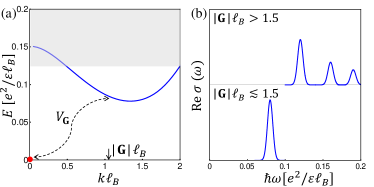
Figure 2: (Color online) Schematic illustration of the perturbation theory analysis. (a)Energy spectrum of Coulomb-only model at filling factor 1/3. The red dot represents the $\nu=1/3$ Laughlin incompressible ground state, the blue line marks the magneto-roton mode and the gray bar the excitation continuum. In the presence of a moiré superlattice potential, the perturbed ground state contains admixtures of unperturbed excited states at momenta $\mathbb{G}$. This admixture enables intra-LL optical response. (b) Schematic illustration of the optical conductivity. When perturbation theory applies and $|\mathbb{G}|\ell_{B}$ is close to 1.5, the SMA is accurate. Thus the intra-LL optical response is dominated by a single peak. When $|\mathbb{G}|\ell_{B}>1.5$, weaker optical responses are expected at multiple frequencies. Tuning $|\mathbb{G}|$ provides a momentum-resolved spectroscopy of FQH excitations.

IV Single Mode Approximation

To illustrate how moiré assisted optical absorption in the quantum Hall regime can be interpreted, we focus on the $\nu=1/m$ case for which the fractional quantum Hall gaps are largest and the simplifying single mode approximation (SMA) is accurate. When the SMA applies, a single collective mode exhausts a large fraction of the oscillator strength available at a particular wavevector, i.e. only one state at wavevector $\mathbb{k}$ has a significant value of $\langle\Psi_{\mathbb{k},n}^{(0)}|\bar{\rho}_{\mathbb{k}}|\Psi_{0}^{(0)}\rangle$ and that state can therefore be approximated by

$$|\phi_{\mathbb{k}}^{(0)}\rangle=\frac{1}{\sqrt{N\bar{s}_{0}(\mathbb{k})}}\bar{\rho}_{\mathbb{k}}|\Psi_{0}^{(0)}\rangle,$$ (23)

where $\bar{s}_{0}(\mathbb{k})$ is the static structure factor defined in Eq.(20). It follows that the long wavelength dynamic structure factor satisfies

$$S(\mathbb{q},\epsilon)\approx\sum_{\mathbb{G}}\Big{|}\frac{V_{\mathbb{G}}\langle\Psi_{0}^{(0)}|\bar{\rho}_{\mathbb{q}+\mathbb{G}}^{\dagger}\bar{\rho}_{\mathbb{q}}\bar{\rho}_{\mathbb{G}}|\Psi_{0}^{(0)}\rangle}{N\Delta_{\mathbb{G}}\sqrt{\bar{s}_{0}(\mathbb{q}+\mathbb{G})}}\Big{|}^{2}\delta(\epsilon-\Delta_{\mathbb{q}+\mathbb{G}}),$$ (24)

where $\Delta_{\mathbb{G}}$ is the Coulomb energy difference between $|\phi_{\mathbb{G}}^{(0)}\rangle$ and $|\Psi_{0}^{(0)}\rangle$, and

$$\frac{\langle\Psi_{0}^{(0)}|\bar{\rho}_{\mathbb{q}+\mathbb{G}}^{\dagger}\bar{\rho}_{\mathbb{q}}\bar{\rho}_{\mathbb{G}}|\Psi_{0}^{(0)}\rangle}{N\bar{s}_{0}(\mathbb{q}+\mathbb{G})}\approx i\ell_{B}^{2}(\mathbb{q}\times\mathbb{G})\cdot\hat{z}.$$ (25)

Therefor the dynamic structure factor to second order in both $V_{\mathbb{G}}$ and $|\mathbb{q}|$ is:

$$S(\mathbb{q},\epsilon)\approx\frac{1}{2}\sum_{\mathbb{G}}\ell_{B}^{4}|\mathbb{q}|^{2}|\mathbb{G}|^{2}\frac{|V_{\mathbb{G}}|^{2}}{\Delta_{\mathbb{G}}^{2}}\bar{s}_{0}(\mathbb{G})\delta(\epsilon-\Delta_{\mathbb{G}}).$$ (26)

Applying Eq.(10) then yields the following remarkably simple expression for the real part of optical conductivity:

$$\text{Re}\sigma(\omega)\,\approx\,\frac{N}{4N_{\phi}}\frac{e^{2}}{\hbar}\sum_{\mathbb{G}}\ell_{B}^{2}|\mathbb{G}|^{2}\frac{|V_{\mathbb{G}}|^{2}}{\Delta_{\mathbb{G}}}\bar{s}_{0}(\mathbb{G})\delta(\hbar\omega-\Delta_{\mathbb{G}}).$$ (27)

Since linear response of $\langle\bar{\rho}_{\mathbb{G}}\rangle_{0}$ to the moiré potential in the SMA is

$$\langle\bar{\rho}_{\mathbb{G}}\rangle_{0}\approx-2N\frac{V_{\mathbb{G}}^{*}}{\Delta_{\mathbb{G}}}\bar{s}_{0}(\mathbb{G}),$$ (28)

Eq. (27) satisfies the $f-$sum rule of Eq.(17). The perturbation theory and SMA are schematically demonstrated in Fig. 2.

V Discussion of Experimental Implications

FQH states at filling factors $1/3$, $2/3$, $4/3$ and $5/3$ have been observed in moiré-patterned graphene on a hBN substrate using capacitanceHunt13 and transportDean15 measurement. Our theory predicts that if light absorption measurements were performed in these samples, they would have a finite intra LL signal, providing the first truly spectroscopic probe of fractional quantum Hall collective excitations. Intra-LL collective excitations have a typical energy $\sim 0.1e^{2}/(\varepsilon\ell_{B})$, which is about $10$ meV ( in the THz frequency range ) at 35T if we use $\varepsilon=3.5$ for the effective dielectric constant. In the SMA [Eqs. (26) and (27)] the excited states at wave vectors $\mathbb{G}$ saturate the $f-$sum rule. The SMA is particularly accurate for the Laughlin state when $\mathbb{G}$ is close to the wave vector of the magneto-roton minimum, and perturbation theory requires $|V_{\mathbb{G}}|$ to be small compared to $\Delta_{\mathbb{G}}$. For $\nu=p/3$ Laughlin states, the roton minimum is located around $k\ell_{B}\sim 1.5$. In aligned graphene/hBN the moiré pattern has a period of 14nm. $|\mathbb{G}|\ell_{B}$ is then about 2.2 at 35T, exceeding the value at which the single-mode-approximation is most accurate and opening a door to the poorly understood crossover between magneto-roton collective modes and fractional particle-hole excitations.

The FQH effect in graphene is enriched by spin and valley degrees of freedomWu14 ; Wu15 . For $N=0$ LLs, electron states in opposite valleys are localized on opposite sublattices. Because the moiré potential of graphene on hBNJung15 is sublattice dependent when projected onto the lowest Landau level, THz absorption could also be used to detect valley polarization.

Twisted TMD bilayers are another candidate for moiré assisted FQH spectroscopy. Common chalcogen TMD heterjunctions, for example WSe₂/MoSe₂, have particularly long period moiré superlattices when aligned. The lattice constants of WSe₂ and MoSe₂ have a mismatch of only $0.1\%\sim 0.2\%$Xiao12 , much smaller that for graphene/hBN. The recent observation of Shubnikov-de Haas oscillations and quantum Hall statesTutuc16 in high mobility holes in monolayer WSe₂ promises the future realization of FQH states. Some differences between TMD bilayers and graphene/hBN could prove interesting because: (1)The N=0 hole LLs of WSe₂ and MoSe₂ have neither spin nor valleyLi13 degeneracy, due to a combination of broken inversion symmetry and strong spin-orbit coupling,Xiao12 simplifying theoretical models and the interpretation of any signals that are observed. (2)The moiré potential is expected to be weakerWu16 , providing stronger justification for the perturbative interpretation we propose, because a TMD monolayer consists of three atomic layers with low-energy electrons located primarily in the middle layer. The moiré potential in TMDs can be tuned by an electric displacement field that is perpendicular to the bilayers. (3) Because of the small lattice constant mismatches of common chalcogen TMD heterjunctions $|\mathbb{G}|\ell_{B}$ can be tuned across the roton minimum of the $1/3$ Laughlin using convenient twist angles. For example using a twist angle of $\sim 0.9^{\circ}$ between WSe₂/MoSe₂ in a 35T magnetic field, $|\mathbb{G}|\ell_{B}$ is close to 1.5. This property should allow the roton minimum dispersion to be measured accurately.

We have assumed that the moiré potential is weak so that FQH states survive. When such assumption breaks down, there can be phase transitions between FQH and Wigner crystal states.Ashley We have mainly focused on Laughlin states. It will be at least equally interestingSon2015 ; Geraedts2106 to probe FQH states at filling factors close to 1/2 optically, since these states are less well understood theoretically.

VI Acknowledgment

Work at Austin was supported by the Department of Energy, Office of Basic Energy Sciences under contract DE-FG02-ER45118 and by the Welch foundation under grant TBF1473. The work of FW at Argonne National Laboratory was supported by the Department of Energy, Office of Science, Materials Sciences and Engineering Division.

References

- (1) A.H. MacDonald, arXiv:cond-mat/9410047 (1994).
- (2) B. Hunt et al., Science 340, 1427 (2013).
- (3) C. R. Dean et al., Nature 497, 598 (2013).
- (4) G. L. Yu et al., Nature Physics 10, 525 (2014).
- (5) L. Wang, Y. Gao, B. Wen, Z. Han, T. Taniguchi, K. Watanabe, M. Koshino, J. Hone, and C. R. Dean, Science 350, 1231 (2015).
- (6) K. Kim, A. DaSilva, S. Huang, B. Fallahazad, S. Larentis, T. Taniguchi, K. Watanabe, B. J. LeRoy, A. H. MacDonald, and E. Tutuc, submitted.
- (7) S. M. Girvin, A. H. MacDonald, and P. M. Platzman, Phys. Rev. Lett. 54, 581 (1985); Phys. Rev. B 33, 2481 (1986).
- (8) F. D. M. Haldane and E. H. Rezayi, Phys. Rev. Lett. 54, 237 (1985).
- (9) Th. Jolicoeur, arXiv:1610.04477.
- (10) D.-H. Lee and S.-C. Zhang, Phys. Rev. Lett. 66, 1220 (1991).
- (11) G. Dev and J. K. Jain, Phys. Rev. Lett. 69, 2843 (1992).
- (12) F. D. M. Haldane, arXiv:0906.1854.
- (13) B. Yang, Z.-X. Hu, Z. Papić, and F. D. M. Haldane, Phys. Rev. Lett. 108, 256807 (2012).
- (14) J. Maciejko, B. Hsu, S. A. Kivelson, Y. J. Park, and S. L. Sondhi, Phys. Rev. B 88, 125137 (2013).
- (15) A. Pinczuk, B. S. Dennis, L. N. Pfeiffer, and K. West, Phys. Rev. Lett. 70, 3983 (1993).
- (16) M. Kang, A. Pinczuk, B. S. Dennis, L. N. Pfeiffer, and K. W. West, Phys. Rev. Lett. 86, 2637 (2001).
- (17) C. F. Hirjibehedin, I. Dujovne, A. Pinczuk, B. S. Dennis, L. N. Pfeiffer, and K. W. West, Phys. Rev. Lett. 95, 066803 (2005).
- (18) U. Wurstbauer, K. W. West, L. N. Pfeiffer, and A. Pinczuk, Phys. Rev. Lett. 110, 026801 (2013).
- (19) The moiré Hamiltonian for graphene on hBN is a spatially periodic matrix operator that acts on sublattice degrees of freedom. See for example Ref. Jung14, . However, because lowest LL wavefunctions exist purely on one sublattice only the potential on that sublattice is relevant for FQH physics.
- (20) R. Bistritzer and A.H. MacDonald, PNAS 108, 12233 (2011).
- (21) J. R. Wallbank, A. A. Patel, M. Mucha-Kruczyński, A. K. Geim, and V. I. Fal’ko, Phys. Rev. B 87, 245408 (2013).
- (22) J. Jung, A. Raoux, Z. Qiao, and A. H. MacDonald, Phys. Rev. B 89, 205414 (2014).
- (23) F. D. M. Haldane, Phys. Rev. Lett. 55, 2095 (1985).
- (24) F. Wu, I. Sodemann, Y. Araki, A. H. MacDonald, and Th. Jolicoeur, Phys. Rev. B 90, 235432 (2014).
- (25) F. Wu, I. Sodemann, A. H. MacDonald, and Th. Jolicoeur, Phys. Rev. Lett. 115, 166805 (2015).
- (26) J. Jung, A. M. DaSilva, A. H. MacDonald, and S. Adam, Nature Commun. 6, 6308 (2015).
- (27) D. Xiao, G.-B. Liu, W. Feng, X. Xu, and W. Yao, Phys. Rev. Lett. 108, 196802 (2012).
- (28) B. Fallahazad, H. C. P. Movva, K. Kim, S. Larentis, T. Taniguchi, K. Watanabe, S. K. Banerjee, and E. Tutuc, Phys. Rev. Lett. 116, 086601 (2016).
- (29) X. Li, F. Zhang, and Q. Niu, Phys. Rev. Lett. 110, 066803 (2013).
- (30) F. Wu, T. Lovorn, and A. H. MacDonald, arXiv:1610.03855.
- (31) A. M. DaSilva, J. Jung, and A. H. MacDonald, Phys. Rev. Lett. 117, 036802 (2016).
- (32) D. T. Son, Phys. Rev. X 5, 031027 (2015).
- (33) S. D. Geraedts, M. P. Zaletel, R. S. K. Mong, M. A. Metlitski, A. Vishwanath, O. I. Motrunich, Science 352, 197 (2016).